Introduction
Metamaterial-based sensors are increasingly preferred for a wide range of sensing applications in fields such as biomedical, electrical, chemical, industrial, food quality assessment, and agriculture [Reference Ebrahimi, Withayachumnankul, Al-sarawi and Abbott1, Reference Prakash and Gupta2]. These sensors are valued for their enhanced sensitivity, high-quality factor, simple manufacturing process, and cost-effectiveness [Reference Prakash and Gupta2]. The evaluation of materials can be effectively carried out by analyzing their permittivity, with metamaterial-based sensors serving as a practical tool for this purpose [Reference Chakyar, Simon, Bindu, Andrews and Joseph3]. The determination of a material’s electric permittivity can be achieved by studying the S-parameters of the sensor [Reference Shahzad, Hu, Samad and Ligthart4]. A novel sensor utilizing metamaterials has been specifically developed for this purpose.
Metamaterials were initially introduced by Veselago in 1968, and the Metamaterial-based split ring resonator (SRR) structure was pioneered by Pendry et al. in 1999 [Reference Pendry, Holden, Robbins and Stewart5]. This study utilizes the Complementary Split Ring Resonator (CSRR), which is essentially the inverse of the SRR pattern etched onto the ground plane. The preference for CSRR over SRR is attributed to its higher sensitivity compared to SRR [Reference Albishi, Mirjahanmardi, Ali, Nayyeri, Wasly and Ramahi6]. Previous studies have demonstrated that CSRR outperforms SRR in terms of sensitivity when both structures have equivalent dimensions [Reference Prakash and Gupta2]. Furthermore, the broader fringing electric fields generated by CSRRs, as opposed to SRRs, facilitate the determination of dielectric properties of larger samples [Reference Prakash and Gupta2]. Placing the material under test (MUT) on the ground plane induces a shift in the resonance frequency, enabling the calculation of the MUT’s permittivity based on the sensor’s resonance frequency with the MUT.
Various metamaterial configurations have been developed for diverse applications, with rectangular and circular shapes being particularly common. Through sensitivity analysis, it has been determined that circular sensors exhibit greater responsiveness to changes in the permittivity of the MUT [Reference Govind, Tiwari, Agrawal and Akhtar7] compared to rectangular sensors of equivalent area [Reference Ansari, Jha and Akhtar8]. Additionally, circular CSRR structures are anticipated to have a higher resonant frequency than their rectangular counterparts for the same unit cell area [Reference Boybay and Ramahi9]. The depth of the notch in the S-parameter output is a crucial factor in ensuring accurate measurements. A deeper notch and a higher Q-factor indicate improved sensor precision. A comparative evaluation of sensor performance based on the depth of the notch is presented in Table 1. In the pursuit of developing an innovative metamaterial shape, an octagonal design has been chosen. Following numerous simulations conducted using CST Studio Suite, the final sensor configuration is illustrated in Fig. 1(b).
Different sensor patterns comparison based on depth notch

Table 1 Long description
Comparison of resonator sensor topologies by resonant frequency and S21 notch depth measured without the material under test. Notch depths span from about minus 11 dB for a rectangular SRR at 2.1 GHz to minus 62.08 dB for a dual-band CSSRR at 5.35 GHz, the strongest notch in the list. Multi-band circular CSRR reports approximate notch depths near minus 22 dB at 2.45 GHz, minus 28 dB at 3.8 GHz, and minus 30 dB at 5.8 GHz. Dual-band CSSRR also shows a second resonance at 8.06 GHz with a shallower minus 19.06 dB notch. Single-band designs cluster around the mid minus teens to high minus twenties, including circular CSRR at 6.01 GHz with minus 31.157 dB, rectangular microfluidic CSRR at 2.02 GHz with minus 24 dB, and CSRR at 2.461 GHz with minus 27 dB. This work’s octagonal CSRR is dual-band, with minus 25 dB at 2.37 GHz and a deeper minus 38 dB at 4.88 GHz, outperforming many single-band entries but not the deepest CSSRR case. Several values are marked approximate, so small differences between close notch depths may not be meaningful.
(a) Layers of sensor. (b) Designed sensor with parameters.

Figure 1 Long description
The diagram consists of two main parts. The first part shows a cross-sectional view of a microstrip resonator sensor, illustrating three layers: the top layer labeled microstrip line, the middle layer labeled substrate and the bottom layer labeled ground plane. This configuration forms the sensing structure, where the microstrip line on the substrate over the ground plane enables resonance-based measurements. The second part displays a top-view layout of the resonator sensor, featuring concentric rings with gaps and connecting segments. The layout includes lettered parameters a through k, which represent various dimensions such as gap width, ring radius and trace width, although no numeric values or units are provided. A magnified circular view highlights the detailed arrangement of these concentric rings, emphasizing their role in the sensor′s function. The diagram illustrates how the microstrip pattern interacts with the substrate and ground plane to form a resonator sensor used for precise measurements based on resonance characteristics.
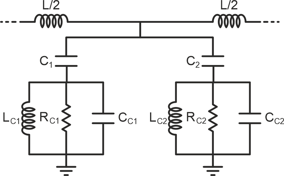
Equivalent circuit model of the CSRR sensor.

Figure 2 Long description
The circuit model includes two parallel branches, each with an inductor labeled L subscript C1 and L subscript C2 and a resistor labeled R subscript C1 and R subscript C2. Each branch is connected to a capacitor labeled C subscript C1 and C subscript C2. The branches are connected to a central line with capacitors C subscript 1 and C subscript 2. Inductors labeled L over 2 are connected at both ends of the central line, leading to external connections. No ratings are shown for any components.
This sensor is specifically engineered to function on two separate frequency bands. Utilizing multiband sensing serves to improve the reliability of sensing by offering sensors that possess high sensitivity and quality factors. Furthermore, variations in frequency shifts may result in identical outcomes for different mixtures; therefore, measurements conducted at a constant frequency are only capable of distinguishing chemicals based on this shift, thereby constraining the accuracy of identification [Reference Zhou, Hu, Yang, Chen, Ji, Chen, Chen, Yang and Mu10].
Sensor design
Based on previous studies, circular CSRR sensors demonstrate a deeper resonance notch compared to their rectangular counterparts. However, structures with sharp edges exhibit stronger localized electric fields around these regions, resulting in enhanced sensitivity. Therefore, in this work, an octagonal CSRR sensor is proposed to combine the advantage of the circular geometry with the enhanced field localization associated with sharp-edged structures [Reference Haq and Koziel16].
The design was intentionally optimized to produce a deeper transmission notch because a larger notch increases the fraction of energy captured by the resonator’s near-field and improves the measurability of the resonance. This yields more pronounced, repeatable resonance peaks with higher frequency-shift sensitivity and better signal-to-noise for extracting the resonant frequency used in the characteristic equation, which in turn improves the accuracy and resolution of the dielectric-constant measurement [Reference Shahzad, Hu, Ali, Raza, Abbas and Ligthart17].
To enhance the performance of the proposed sensor, an optimization process was conducted to achieve an optimal balance among sensitivity, compactness, and fabrication feasibility. In the first stage, a single-resonance CSRR sensor was designed, and a series of parametric sweeps were performed on the critical geometrical parameters, including the split-gap width, number of rings, ring spacing, and conductor line width. After determining the configuration that provided the highest sensitivity and the deepest resonance notch, a second resonant structure was incorporated into the design. Subsequently, additional parametric sweeps were carried out on the inter-structure spacing to finalize the optimized sensor geometry.
To obtain optimal resonator geometry with maximum sensitivity, the design process started from a single octagonal resonator incorporating a notch. First, the notch position along the octagonal contour was systematically evaluated in CST Studio Suite to maximize the resonance frequency shift induced by the dielectric under test, while maintaining a well-defined transmission notch in the S 21 response. After selecting the best notch location, two additional parameters—the octagon linewidth and the notch width—were swept to determine the primary sensor geometry. These parameters directly influence the effective inductance and capacitance of the resonator and therefore control the resonance frequency, notch bandwidth, and quality factor.
To further enhance field confinement and increase the interaction region between the resonator and the MUT, a second octagonal structure, similar to the first but scaled in size, was added to the design. A parametric sweep was then performed to determine the optimum scaling factor and spacing between the two octagonal elements. To further improve sensitivity, a third scaled octagonal element was introduced and optimized using the same procedure.
In addition to linewidth, notch dimensions, and spacing between the octagonal elements, the relative rotation angle between the octagonal structures was found to significantly affect the coupling strength and the resulting S 21 notch characteristics. The best response was obtained when the second octagon was rotated by 180° relative to the other elements, as shown in Fig. 1(b). The same optimization procedure was then applied to the third octagonal element. During the entire optimization procedure, the quality factor was evaluated in order to ensure high sensitivity and is defined as:
 \begin{equation}Q = \frac{{{f_r}}}{{{\text{B}}{{\text{W}}_{ - 3{\text{dB}}}}}}\end{equation}
where  ${f_r}$ is the resonance frequency, and
 ${\text{B}}{{\text{W}}_{ - 3{\text{dB}}}}$ is the −3 dB bandwidth around the resonance.
After obtaining the final resonator geometry, a second resonator was added on the ground plane. The distance between the two resonators was then swept to achieve high sensitivity while preserving a clear and measurable transmission notch. This step is critical because coupling between the two resonators modifies the resonance behavior and can significantly affect both the resonance frequency shift and the overall sensor performance.
The frequency range of 2–10 GHz was selected for this sensor, as it offers good sensitivity while being less susceptible to electromagnetic noise. Moreover, since the inner octagonal section of the smaller resonator is relatively thin, reducing its dimensions excessively would increase fabrication complexity and cost. Therefore, the chosen frequency band represents a suitable compromise between performance, manufacturability, and measurement stability.
The sensor is implemented on a microstrip, as depicted in Fig. 1(a): a trace line on the top, a substrate layer, and a ground plane with metamaterial-inspired shapes etched onto it. The substrate is constructed from low-cost FR4 with a thickness of 0.8 mm, while the two additional layers are made of 0.035 mm copper. The substrate has a length of 70 mm and a width of 30 mm. Additionally, the dimensions are specified as follows: a = 12 mm, b = 6 mm, c = d = f = 3 mm, e = 1.6 mm, g = 0.9 mm, i = j = 4 mm, and k = 1.9 mm, and the smaller resonator shape has dimensions exactly half of the larger one. The resonant frequencies of the sensor are 4.88 GHz and 2.37 GHz.
An equivalent circuit model was developed to provide physical insight into the resonance mechanism of the proposed sensor and to support the design and optimization procedure. In the proposed circuit, the two transmission notches observed in the  ${S_{21}}$response are represented by two resistor-inductor-capacitor (RLC) resonant branches, where each RLC branch corresponds to one resonant element (or resonance mode) of the sensor structure. The inductance and capacitance values model the effective current path and electric-field concentration of the resonators, while the resistive terms account for conductor and dielectric losses. The coupling between the microstrip line and the resonators is modeled through coupling capacitances, which mainly determine the notch depth and bandwidth. This circuit model provides a compact representation that enables interpretation of the main geometrical parameters (notch width, linewidth, spacing, and rotation angle) in terms of effective circuit parameters and allows direct validation against full-wave CST results.
Figure 2 illustrates the equivalent circuit of the proposed sensor [Reference Baena, Bonache, Martin, Sillero, Falcone, Lopetegi, Laso, Garcia-Garcia, Gil, Portillo and Sorolla18].
Simulation
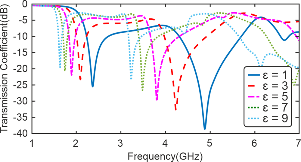
At the resonance of the CSRR, significant fringing electric fields are generated in the ground plane, providing an additional method to determine dielectric properties [Reference Lee and Yang19]. The electromagnetic energy, concentrated in a confined area near the substrate at the resonant frequency, is used to determine dielectric properties [Reference Lim, Kim and Hong20]. The most intense electric field is established between the microstrip line and the ground plane. As shown in Fig. 3, the concentration of the electric field near each resonator results in the formation of notches in the transmission coefficient plot at the resonant frequency. The positioning of the MUT can be more accurately determined by pinpointing the location of the strong electric field. Placing the MUT on the sensor causes a shift in these notches. The transmission coefficient is depicted in Fig. 4 for various MUTs with differing permittivity. The shift of the notch from εr = 1 to εr = 3 is 640 MHz for the smaller resonator with a resonant frequency of 4.88 GHz, demonstrating the high sensitivity of the sensor. Additionally, the quality factor for the 4.88 GHz band is 81.3, signifying a remarkable quality factor for a sensor employing an FR4 substrate. Furthermore, the frequency shift for the larger resonator with the same values of εr is 277 MHz, and the Q-factor is equal to 41.5 dB.
(a) Electric field on the ground plane at 2.37 GHz. (b) Electric field on the ground plane at 4.88 GHz.

Simulated transmission response of the sensor in different permittivities.

Figure 4 Long description
Transmission Co-efficient(dB) Frequency(GHz) A line graph with five plotted curves and a legend. The x-axis is labeled Frequency(GHz) and runs from 1 to 7 with tick marks at 1, 2, 3, 4, 5, 6 and 7. The y-axis is labeled Transmission Co-efficient(dB) and runs from 0 at the top down to minus 40 at the bottom, with tick marks at 0, minus 5, minus 10, minus 15, minus 20, minus 25, minus 30, minus 35 and minus 40. The legend lists five series: e equals 1, e equals 3, e equals 5, e equals 7 and e equals 9. e equals 1: A curve near 0 decibel from about 1 to about 1.8 gigahertz, then a deep notch near about 2.0 gigahertz reaching about minus 25 decibel, then rises toward about minus 5 decibel by about 3.0 gigahertz. A second deep notch occurs near about 5.0 gigahertz reaching about minus 35 decibel, then the curve rises toward about minus 5 decibel by about 6.0 gigahertz and approaches near 0 decibel by about 7.0 gigahertz. e equals 3: A curve near 0 decibel from about 1 to about 1.8 gigahertz, then a notch near about 2.0 gigahertz reaching about minus 30 decibel, then rises to around minus 5 to minus 10 decibel by about 3.0 gigahertz. Another notch appears near about 4.6 to 4.8 gigahertz reaching about minus 30 decibel, then rises toward about minus 5 decibel by about 6.0 gigahertz. e equals 5: A curve near 0 decibel from about 1 to about 1.8 gigahertz, then a notch near about 2.0 gigahertz reaching about minus 30 decibel. A second notch appears near about 4.2 to 4.4 gigahertz reaching about minus 30 decibel, then the curve rises toward about minus 5 decibel by about 6.0 gigahertz. e equals 7: A curve near 0 decibel from about 1 to about 1.8 gigahertz, then a notch near about 2.0 gigahertz reaching about minus 30 decibel. A second notch appears near about 3.9 to 4.1 gigahertz reaching about minus 30 decibel, then the curve rises toward about minus 5 decibel by about 6.0 gigahertz. e equals 9: A curve near 0 decibel from about 1 to about 1.8 gigahertz, then a notch near about 2.0 gigahertz reaching about minus 30 decibel. A second notch appears near about 3.6 to 3.8 gigahertz reaching about minus 30 decibel, then the curve rises toward about minus 5 decibel by about 6.0 gigahertz.
As illustrated in Fig. 4, an increase in ε causes a reduction in notch depth. Moreover, to prevent band interference, a specific range of permittivity should be selected for measurement. Therefore, an εr of less than 10 should be chosen.
Equivalent circuit parameters of the sensor
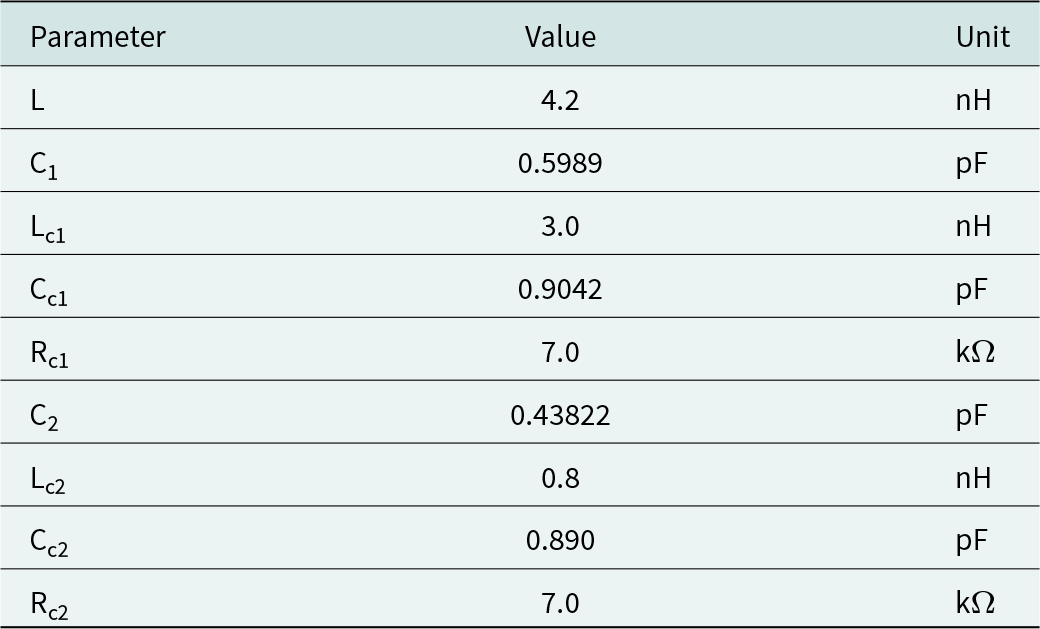
Table 2 Long description
Equivalent circuit component values are provided for a sensor, listing inductance, capacitance, and resistance parameters with units. Inductance values include L at 4.2 nanohenry, Lc1 at 3.0 nanohenry, and Lc2 at 0.8 nanohenry, making Lc2 the smallest inductance. Capacitance values include C1 at 0.5989 picofarad and C2 at 0.43822 picofarad, with C2 lower than C1. Coupling capacitances are Cc1 at 0.9042 picofarad and Cc2 at 0.890 picofarad, which are close in magnitude, with Cc1 slightly higher. Resistance values are Rc1 and Rc2, both 7.0 kiloohm, indicating matching resistive elements in the two branches. Values are reported as single numbers without uncertainty or test conditions, so comparisons are limited to the listed magnitudes.
Temperature is another parameter that can influence this observation and cause variations in the results. Temperature rise results in an increase in the permittivity of FR4 [Reference Paghi, Trupiano, Puglia, Burgaud, De Simoni, Greco and Giazotto21, Reference Miller22], which causes variations in the resonance frequency and decreases the accuracy of the sensor. Therefore, all measurements should be obtained at a constant temperature. With additional simulations involving different MUTs, a relationship between permittivity and frequency can be derived. A polynomial function is considered to fit the simulation data:
 \begin{equation}{{\varepsilon }_r} = {A_1}{f^2} + {A_2}f + {A_3}\end{equation}
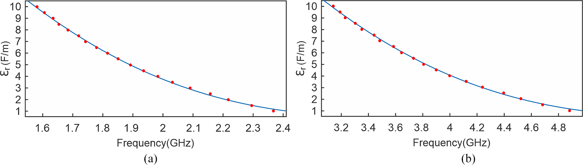
Simulation data are processed in MATLAB, yielding a quadratic equation for each resonator.
The resonance frequency decreases as the dielectric constant increases. This behavior is expected, since the MUT increases the effective capacitance of the CSRR structure, thereby reducing the resonance frequency according to the inductance-capacitance (LC) resonance principle.
In Fig. 5, the quadratic equation fitted to the simulation data is illustrated. For the larger resonator with 2.37 GHz resonant frequency, the coefficients are A1 = 9.404, A2 = −48.2, and A3 = 62.57, while for the smaller resonator, the coefficients are A1 = 2.001, A2 = −21.05, and A3 = 56.21.
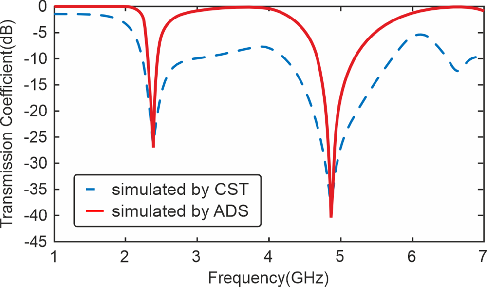
To validate the proposed equivalent circuit model, the transmission coefficient obtained from the circuit simulation in Advanced Design System (ADS) is compared with the full-wave electromagnetic simulation performed in CST Studio Suite, as shown in Fig. 6. The equivalent circuit successfully reproduces the two resonance notches and accurately predicts the resonance frequencies at 2.37 GHz and 4.88 GHz, in excellent agreement with the CST results. The extracted lumped-element values used in the circuit model are summarized in Table 2 and were obtained by fitting the ADS response to the CST  $\left| {{S_{21}}} \right|$ curve, where the RLC parameters were adjusted to match the resonance frequencies and bandwidth, while the coupling capacitances were tuned to reproduce the notch depth. Minor differences in notch depth and out-of-resonance behavior can be attributed to higher-order parasitic effects, radiation, and distributed coupling mechanisms that are inherently captured in the full-wave simulation but are not fully represented in the lumped-element circuit model. Overall, the comparison confirms that the proposed circuit model provides an accurate representation of the sensor resonance behavior and can be used to support the design analysis.
(a) Fitted curve to larger resonator’s simulation data. (b) Fitted curve to smaller resonator’s simulation data.

Comparison of the transmission coefficient  $\left| {{S_{21}}} \right|$ obtained from full-wave CST simulation and the proposed equivalent circuit model simulated in ADS.

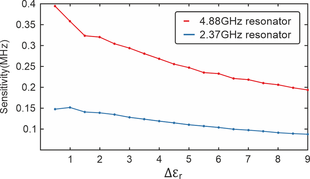
Calculated sensitivity of each band versus relative permittivity variation ( ${\varepsilon _r}$).

(a) Fabricated sensor connected to network analyzer. (b) Fabricated sensor top view.

Measurement results of the fabricated sensor with different MUTs.

Figure 9 Long description
The multi-line graph compares transmission coefficients in decibels on the vertical axis, ranging from negative 45 to 0, with frequency in gigahertz on the horizontal axis, ranging from 1 to 7. The graph includes lines for simulation, air, teflon, plexi, epoxy and glass. Each line is visually distinguished by different styles: simulation is solid, air is dashed, teflon is dotted, plexi is dash-dot, epoxy is dash-dot-dot and glass is dotted. The graph shows variations in transmission coefficients across the frequency range. Notable points include peaks and troughs for each material. For example, teflon shows a significant dip around 3.5 gigahertz, while epoxy has a peak near 5 gigahertz. The purpose of the graph is to illustrate how different materials affect transmission across frequencies, highlighting which materials have better or worse transmission characteristics. This information is crucial for understanding material performance in specific frequency bands.
To evaluate the sensing performance, a sensitivity analysis was carried out by investigating the resonance frequency variation of the proposed CSRR sensor when different dielectric materials were placed on the sensitive region. The sensitivity is defined as the change in resonance frequency with respect to the variation in the relative permittivity of the MUT, and it is expressed as:
 \begin{equation}Sensitivity = \frac{{\Delta {f}}}{{\Delta {{\varepsilon }_r}}}\end{equation}
where  $\Delta {f_r} = {f_{r0}} - {f_r}$ is the resonance frequency shift,
 ${f_{r0}}$ is the resonance frequency corresponding to the reference condition (no load), and
 ${f_r}$ is the resonance frequency in the presence of the MUT.
 $\Delta {\varepsilon _r}$ represents the relative permittivity change between two consecutive MUT cases. A higher sensitivity indicates that smaller variations in dielectric properties can be detected.
The sensitivity corresponding to selected permittivity values within the investigated range was computed using (3), and the results are reported in Fig. 7.
Fabrication and measurement
The sensor was constructed according to the specifications provided in the sensor design section, with the impedance of the microstrip line standardized at 50 Ω. Figure 8(a) depicts the experimental setup, illustrating the sensor’s connection to a network analyzer. Furthermore, Fig. 8(b) displays the ground plane of the manufactured sensor.
The dimensions of the MUT play a crucial role in ensuring the accuracy of measurements. When the MUT sufficiently covers the area surrounding the resonators, the outcomes are relatively consistent. However, for enhanced precision, it is recommended to maintain uniform measurements. These measurements were obtained through simulations involving various MUT sizes, which were reflected in both the simulation outcomes and the practical measurements. In this particular measurement, the MUT dimensions were set at 60 × 20 × 3 mm. Consistent environmental conditions are essential to ensure accurate results and prevent interference with the field distribution around the test probe during measurements [Reference Chakyar, Simon, Bindu, Andrews and Joseph3]. Figure 9 illustrates the output from the network analyzer, highlighting the alignment between simulation and measurement results. The frequencies obtained from the measurements were incorporated into the formula derived from simulations, and the results are outlined in Table 3.
The imaginary part of permittivity can also be derived from the loss tangent. To calculate the loss tangent, the quality factor must first be determined, as given by:
 \begin{equation}\frac{1}{{{Q_L}}} + \frac{1}{{Q_0}} = \tan \delta \end{equation}
Where Q0 and QL signify the quality factors of the sensor without and with the sample. ε′′ is calculated using the following equation:
 \begin{equation}{\varepsilon ^{''}} = {\varepsilon _r} \cdot \tan \delta \end{equation}
Where εr is derived from the measured data of the sensor. The ε′′ values for both resonators are shown in Table 4.
Measured relative permittivity values
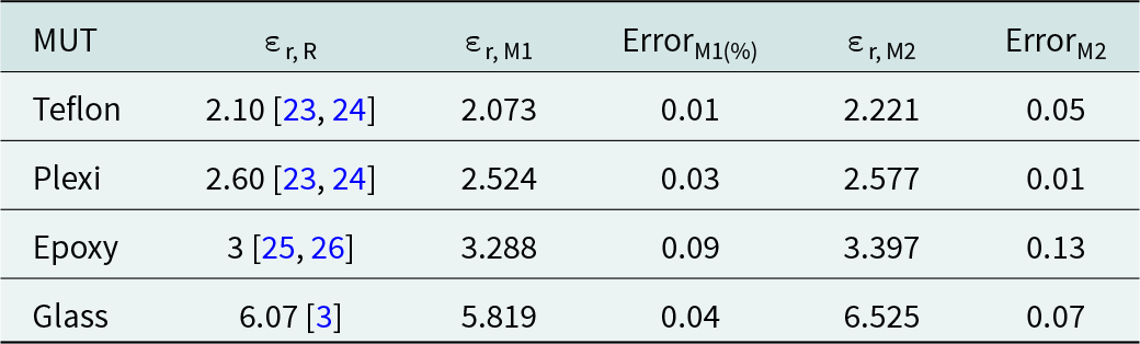
Table 3 Long description
Relative permittivity values are listed for four materials, comparing a published reference against two measured results from a smaller resonator and a larger resonator, each with a percent error. Teflon has a reference of 2.10, measured as 2.073 with 0.01 percent error for the smaller resonator and 2.221 with 0.05 percent error for the larger resonator. Plexi has a reference of 2.60, measured as 2.524 with 0.03 percent error and 2.577 with 0.01 percent error. Epoxy has a reference of 3.0, measured as 3.288 with 0.09 percent error and 3.397 with 0.13 percent error. Glass has a reference of 6.07, measured as 5.819 with 0.04 percent error and 6.525 with 0.07 percent error. Across materials, the larger resonator tends to produce higher measured permittivity than the smaller resonator, except that glass shifts from below the reference with the smaller resonator to above the reference with the larger resonator. Errors are smallest for teflon and plexi and largest for epoxy, indicating the epoxy measurements deviate most from the reference among the four materials.
*εr, R is reference value of dielectric constant; εr, M1 and εr, M2 represent measured permittivity of smaller and larger resonator; ErrorM1 and ErrorM2 represent error of measurements
Measured loss tangent and imaginary part of permittivity values*
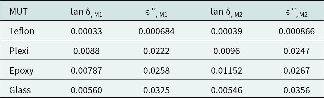
Table 4 Long description
Option 1: Materials compared by loss tangent and imaginary permittivity using two measurement methods labeled M1 and M2. Teflon is lowest in both methods, with loss tangent about 0.00033 in M1 and 0.00039 in M2, and imaginary permittivity about 0.000684 in M1 and 0.000866 in M2. Plexi and epoxy have much higher loss tangents, around 0.0088 and 0.00787 in M1, rising to about 0.0096 and 0.01152 in M2. Glass has moderate loss tangent near 0.00560 in M1 and 0.00546 in M2, but the highest imaginary permittivity, about 0.0325 in M1 and 0.0356 in M2. Across materials, M2 generally reports slightly higher imaginary permittivity than M1, while loss tangent changes are small except for epoxy, which increases notably in M2. Imaginary permittivity can help distinguish materials when their real permittivity values are similar, so comparisons should consider that identification context.
The ε′ can be used for materials with similar permittivity constants. For similar permittivity constants, ε′ can be used for more accurate material identification.
Conclusion
An effective microwave sensor was developed, modeled, produced, and evaluated for material analysis purposes. Following an examination of various sensor configurations, a dual-band octagonal CSRR was devised. The experimental findings closely matched the results obtained through simulation. The sensor demonstrated high sensitivity and a notable notch depth of −38 dB for the smaller resonator and −25 dB for the larger resonator, which is considered impressive considering the utilization of an FR4 substrate. A polynomial function was derived to describe the correlation between the sensor’s permittivity and frequency. The results demonstrate that the proposed CSRR sensor provides a consistent and measurable frequency shift for different dielectric materials. The frequency shift exhibits a monotonic dependence on the permittivity, confirming that the sensor can distinguish materials with different dielectric constants.
Acknowledgements
This work is supported in part by Shahid Rajaee Teacher Training University.
Competing interests
The authors have no competing interests to declare that are relevant to the content of this article.

Ali Zolfagharian was born in Tehran, Iran, in 1997. He received his B.Sc. degree in Electrical Engineering from Shahid Rajaee Teacher Training University, Tehran, Iran, in 2020. He is currently working as an electrical engineer specializing in the optimization of energy systems and uninterruptible power supplies (UPS).

Fateme Geran was born in Qaem Shahr, Iran, in 1977. She received her BSc degree in Electrical Engineering (Telecommunication) from Tehran University, Tehran, Iran, in 1999. Also, she received her MSc and PhD degrees in Electrical Engineering (Telecommunication) from Tarbiat Modares University, Tehran, Iran, in 2003 and 2009, respectively. She is currently an assistant professor in the Faculty of Electrical Engineering at Shahid Rajaee Teacher Training University, Tehran, Iran. Her research interest fields are antenna, RF subsystems in microwave and mm-wave Bands and RF energy harvesting.