1. Introduction
In this work we shall consider a two-dimensional body that moves horizontally from right to left at a constant speed
 $c$
in a channel of finite depth
 $h$
. We assume the fluid to be incompressible and inviscid, the flow to be irrotational. Also, we suppose that in the body frame of reference the flow is steady. Then the wave train generated by the body also moves from right to left with the same velocity
 $c$
. In the body frame of reference we introduce Cartesian coordinates with the
 $x$
-axis lying on the bottom of the channel and the
 $y$
-axis directed vertically upward. In this coordinate system, far upstream we have a uniform stream with velocity
 $c$
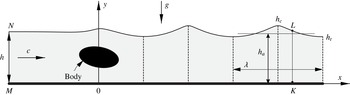
and far downstream a train of steady periodic waves (figure 1).
In spite of the absence of energy dissipation, due to the generation of waves (momentum losses) the body experiences a wave resistance
 $R_{w}$
, by which we mean the horizontal component of the resultant of the pressure forces on the body. It is to be noted that in the nonlinear wave theory the wave resistance so defined does not always vanish when the wave train far downstream degenerates to a uniform flow (see e.g. Binder, Vanden-Broek & Dias Reference Binder, Vanden-Broek and Dias2009, p. 187).
In two-dimensional cases the determination of this resistance from properties of the wave train has been the subject of several investigations. The linear theory was first presented by Lord Kelvin (1887). He derived that the wave resistance
 $$\begin{eqnarray}R_{w}=\frac{1}{4}{\it\rho}ga^{2}\left[1-\frac{4{\rm\pi}h/{\it\lambda}}{\sinh (4{\rm\pi}h/{\it\lambda})}\right],\end{eqnarray}$$
where
 ${\it\rho}$
is the fluid density,
 $g$
is the acceleration due to gravity,
 ${\it\lambda}$
is the wavelength and
 $a=(h_{c}-h_{t})/2$
is the wave amplitude (one half the vertical distance from the crest to the trough). For deep water this formula simplifies and takes the form
 $$\begin{eqnarray}R_{w}={\textstyle \frac{1}{4}}{\it\rho}ga^{2}.\end{eqnarray}$$
Sketch of a steady free-surface flow over a body.

Wehausen & Laitone (Reference Wehausen, Laitone and Truesdell1960, p. 460) by means of an energy balance equation have derived an exact resistance formula for three-dimensional bodies. In the two-dimensional case their result is as follows:
 $$\begin{eqnarray}R_{w}=\frac{{\it\rho}}{2}\int _{0}^{{\it\eta}(x)}[v_{y}^{2}-(v_{x}-c)^{2}]\,\text{d}y+\frac{{\it\rho}g}{2}[{\it\eta}(x)-h]^{2}.\end{eqnarray}$$
Here
 $v_{x}(x,y)$
and
 $v_{y}(x,y)$
are the components of the velocity vector in the steady flow,
 $y={\it\eta}(x)$
is the equation of the free surface, and the integration is along any vertical segment located behind the body.
Duncan (Reference Duncan1983) was the first to notice that an exact value of wave resistance can be expressed in terms of some integral far-downstream wave properties. For the infinite depth case, using the horizontal-momentum equation and some results by Longuet-Higgins (Reference Longuet-Higgins1975), Duncan (Reference Duncan1983) deduced that
 $$\begin{eqnarray}R_{w}=cI+3V-4T,\end{eqnarray}$$
where
 $I$
is the mean impulse:
 $$\begin{eqnarray}I=\frac{{\it\rho}}{{\it\lambda}}\mathop{\iint }_{{\it\Omega}_{z}\hspace{6.0pt}}(c-v_{x})\,\text{d}x\,\text{d}y,\end{eqnarray}$$
and
 $V$
and
 $T$
are the mean potential and kinetic energies, respectively:
 $$\begin{eqnarray}V=\frac{{\it\rho}g}{2{\it\lambda}}\int _{x}^{x+{\it\lambda}}[{\it\eta}(x)-h_{a}]^{2}\,\text{d}x,\quad T=\frac{{\it\rho}}{2{\it\lambda}}\mathop{\iint }_{{\it\Omega}_{z}\hspace{6.0pt}}[(v_{x}-c)^{2}+v_{y}^{2}]\,\text{d}x\,\text{d}y.\end{eqnarray}$$
In (1.5), (1.6) the domain
 ${\it\Omega}_{z}$
is one wave period,
 $h_{a}$
is the height of the mean level of waves:
 $$\begin{eqnarray}h_{a}=\frac{1}{{\it\lambda}}\int _{x}^{x+{\it\lambda}}{\it\eta}({\it\xi})\,\text{d}{\it\xi}.\end{eqnarray}$$
It is to be noted that the above definitions of
 $I$
,
 $T$
,
 $V$
and
 $h_{a}$
are valid for finite and infinite depths, but for infinite depth the location of the
 $x$
-axes is arbitrary.
Numerical results of Longuet-Higgins (Reference Longuet-Higgins1975) and formula (1.4) allowed Duncan to obtain accurate values of the wave resistance for arbitrary wave steepness.
Another important result of Duncan (Reference Duncan1983) is the formula
 $$\begin{eqnarray}R_{w}=\frac{1}{4}{\it\rho}ga^{2}\left[1-\frac{3}{2}\frac{(2{\rm\pi}a)^{2}}{{\it\lambda}^{2}}\right],\end{eqnarray}$$
that generalizes (1.2) up to the fourth power of the amplitude
 $a$
. Equation (1.8) has been obtained by making use of formula (1.3) given above and the third-order Stokes wave theory.
Formula (1.4) is correct only for deep water. The main goal of the present work is to generalize (1.4) for water of finite depth and to obtain numerically accurate values of
 $R_{w}$
for any amplitude and depth. We have established that in the finite depth case
 $$\begin{eqnarray}R_{w}={\textstyle \frac{3}{2}}{\it\rho}g{\it\delta}_{2}^{2}+{\it\rho}(gh-c^{2}){\it\delta}_{1},\end{eqnarray}$$
where
 ${\it\delta}_{1}$
and
 ${\it\delta}_{2}$
are, respectively, the mean and root-mean-square deviations of the free-surface shape far downstream from the undisturbed level
 $h$
:
 $$\begin{eqnarray}{\it\delta}_{1}=\frac{1}{{\it\lambda}}\int _{x}^{x+{\it\lambda}}[{\it\eta}({\it\xi})-h]\,\text{d}{\it\xi},\quad {\it\delta}_{2}^{2}=\frac{1}{{\it\lambda}}\int _{x}^{x+{\it\lambda}}[{\it\eta}({\it\xi})-h]^{2}\,\text{d}{\it\xi}.\end{eqnarray}$$
As one can see from (1.9), to compute the wave resistance
 $R_{w}$
of a body that moves with a constant speed
 $c$
in a channel of depth
 $h$
one needs only to determine two parameters
 ${\it\delta}_{1}$
and
 ${\it\delta}_{2}$
, which have the dimension of length and depend on the shape of the free surface in the far field.
The parameter
 ${\it\delta}_{1}=h_{a}-h$
can be treated as a defect of levels (the difference between the mean level far downstream and the undisturbed level far upstream). The fact that due to nonlinear effects
 $h\neq h_{a}$
was noticed by Whitham (Reference Whitham1962, p. 142) and later was numerically confirmed by Salvesen & von Kerczek (Reference Salvesen and von Kerczek1976, p. 168). In this paper we rigorously prove that, if
 $R_{w}>0$
, then
 ${\it\delta}_{1}=h_{a}-h<0$
.
To pass to the limit
 $h\rightarrow \infty$
in (1.9) we have deduced another representation for
 $R_{w}$
, equivalent to (1.9), namely,
 $$\begin{eqnarray}R_{w}=3V-2T+\frac{3}{2}{\it\rho}g{\it\delta}_{1}^{2}-\frac{{\it\rho}}{2}h{\it\sigma}_{b}^{2},\end{eqnarray}$$
where
 ${\it\sigma}_{b}$
is the root-mean-square velocity at the bottom in the far field:
 $$\begin{eqnarray}{\it\sigma}_{b}^{2}=\frac{1}{{\it\lambda}}\int _{x}^{x+{\it\lambda}}[v_{x}({\it\xi},0)-c]^{2}\,\text{d}{\it\xi}.\end{eqnarray}$$
It follows from (1.11) that in infinitely deep water
 $$\begin{eqnarray}R_{w}=3V-2T,\end{eqnarray}$$
which is equivalent to Duncan’s result (1.4), because
 $cI=2T$
(see Longuet-Higgins Reference Longuet-Higgins1975, p. 159).
By making use of (1.4) Duncan (Reference Duncan1983) has established an important physical limit for the wave resistance of a body in deep water, namely, he demonstrated that
 $R_{w}\leqslant 0.02{\it\rho}c^{4}/g$
. In this paper we show that in water of finite depth
 $R_{w}\leqslant 0.0236{\it\rho}c^{4}/g$
, and to achieve the maximum the body should be towed with a speed of
 $c\approx 0.692\sqrt{gh}$
, creating waves with an amplitude of
 $0.189h$
. Under these conditions the body will generate waves with wavelength
 ${\it\lambda}\approx 3h$
and defect of levels
 ${\it\delta}_{1}\approx -0.034h$
.
It is to be noted that the results for the wave resistance obtained in the paper are correct not only for a body that moves under a free surface, but also for a plate planing on a water surface without spray formation, for a bump on a horizontal bottom or for a free-surface flow over a system of concentrated singularities, such as vortices and doublets. So the results are independent of the type of flow disturbance under the assumption that on the free surface there are no wavebreaking and sprays. The only requirement is that the levels of the bottom far upstream and far downstream of the disturbance are equal.
2. Mathematical formulation of the problem
We denote by
 ${\it\psi}(x,y)$
the stream function of the steady flow; then
 $v_{x}=\partial {\it\psi}/\partial y$
,
 $v_{y}=-(\partial {\it\psi}/\partial x)$
are the components of the velocity vector. Let
 $$\begin{eqnarray}Q=ch,\quad \frac{c^{2}}{2}+gy=R,\end{eqnarray}$$
where
 $Q$
is the volume flux and
 $R$
is the Bernoulli constant. If the pressure
 $p$
is measured from atmospheric (on the free surface
 $p=0$
), then in the entire flow domain the Bernoulli equation is fulfilled:
 $$\begin{eqnarray}\frac{1}{2}(v_{x}^{2}+v_{y}^{2})+gy+\frac{p}{{\it\rho}}=R.\end{eqnarray}$$
The mathematical formulation of the problem is as follows. Find the function
 ${\it\eta}(x)>0$
,
 $x\in (-\infty ,+\infty )$
and the harmonic stream function
 ${\it\psi}(x,y)$
in the domain
 $0\leqslant y\leqslant {\it\eta}(x)$
subject to the boundary conditions
 $$\begin{eqnarray}\displaystyle & \displaystyle {\it\psi}=\left\{\begin{array}{@{}ll@{}}0 & \text{on the bottom }y=0,\\ Q & \text{on the free surface }y={\it\eta}(x),\end{array}\right. & \displaystyle\end{eqnarray}$$
 $$\begin{eqnarray}\displaystyle & \displaystyle {\textstyle \frac{1}{2}}(v_{x}^{2}+v_{y}^{2})+gy=R\quad \text{on the free surface }y={\it\eta}(x), & \displaystyle\end{eqnarray}$$
 $$\begin{eqnarray}\displaystyle & \displaystyle {\it\psi}=\text{const.}\quad \text{on the surface of the body}, & \displaystyle\end{eqnarray}$$
 $$\begin{eqnarray}{\it\eta}(x)\rightarrow h,\quad {\it\psi}(x,y)\rightarrow cy\quad \text{as }x\rightarrow -\infty .\end{eqnarray}$$
In the boundary condition (2.5) the constant on the right-hand side must be determined as a part of the solution to the problem.
Let us introduce the upstream Froude number
 $$\begin{eqnarray}\mathit{Fr}=\frac{c}{\sqrt{gh}}.\end{eqnarray}$$
The flow is called subcritical if
 $\mathit{Fr}<1$
and supercritical if
 $\mathit{Fr}>1$
. According to the linear theory (see Lamb Reference Lamb1932, arts. 245–246), if
 $\mathit{Fr}>1$
, then the function
 ${\it\eta}(x)\rightarrow h$
as
 $x\rightarrow +\infty$
. Hence, in this case there are no waves far downstream. If
 $\mathit{Fr}=1$
, linearized bounded solutions do not exist. If
 $\mathit{Fr}<1$
, then the linear theory predicts that far downstream a train of periodic waves appears, and the length and amplitude of the waves depend on the Froude number
 $\mathit{Fr}$
and the shape of the body.
Thus, according to the linear theory there are only two options for the behaviour of the linearized solutions at the right infinity: either far downstream we have a uniform stream or far downstream we have a train of periodic waves. In solving the nonlinear problem (2.3)–(2.6), it seems to be natural to assume the same. Thus we suppose that for any solution to the problem (2.3)–(2.6) there exists
 ${\it\lambda}>0$
such that
 $$\begin{eqnarray}\lim _{n\rightarrow \infty }{\it\eta}(x+n{\it\lambda})={\it\eta}_{\ast }(x)<\infty ,\quad \lim _{n\rightarrow \infty }{\it\psi}(x+n{\it\lambda},y)={\it\psi}_{\ast }(x,y)<\infty ,\quad n\in \mathbb{N}.\end{eqnarray}$$
It is clear that the functions
 ${\it\eta}_{\ast }(x)$
and
 ${\it\psi}_{\ast }(x,y)$
are
 ${\it\lambda}$
-periodic with respect to
 $x$
and satisfy the boundary conditions (2.3) and (2.4), which means that far downstream there exists a train of periodic waves with wavelength
 ${\it\lambda}$
. The conditions (2.8) also include the case of a uniform stream at the right infinity for which
 $$\begin{eqnarray}{\it\eta}_{\ast }(x)=h_{d}=\text{const.},\quad {\it\psi}_{\ast }(x,y)=c_{d}y,\quad c_{d}=\frac{Q}{h_{d}},\end{eqnarray}$$
where
 $h_{d}$
and
 $c_{d}$
are the depth and speed of this stream. So, the conditions (2.8) cover both options mentioned above, but if equalities (2.9) hold, then the value
 ${\it\lambda}>0$
in (2.8) can be arbitrary.
Conditions (2.8), (2.9) can be justified as follows. It is apparent that far downstream the influence of the disturbing obstruction is negligibly small and the functions
 ${\it\eta}_{\ast }(x)$
and
 ${\it\psi}_{\ast }(x,y)$
must only satisfy the boundary conditions (2.3), (2.4). So far in the nonlinear wave theory three types of solutions to the problem (2.3), (2.4) are known: uniform streams, periodic waves (possibly non-symmetric) and solitary waves. But for the solitary waves the crests are located at infinite distance from the troughs, under which the flows are uniform. Thus, the far-downstream solitary waves do not disturb the far-downstream uniform streams behind the obstruction. This means that for nonlinear problems the conditions (2.8) cover all possibilities.
The formulation of the nonlinear problem (2.3)–(2.6), (2.8) raises an important question of solvability. Existence theorems for problems of such a type were proved by Nalimov (Reference Nalimov1982) (subcritical flow over a small bump on a horizontal bottom) and by Maklakov (Reference Maklakov1997) (subcritical flow past a line vortex of small strength).
If a solution to the problem (2.3)–(2.6), (2.8) satisfies (2.9), then we are able to introduce the downstream Froude number
 $$\begin{eqnarray}\mathit{Fr}_{d}=\frac{c_{d}}{\sqrt{gh_{d}}}.\end{eqnarray}$$
We should note that, strictly speaking, in the definitions (1.5)–(1.7), (1.10) and (1.12) of § 1 we should write the subscript asterisks from the conditions (2.8) for all functions in the integrands to indicate that the functions are computed at the right infinity. But as in § 1, in what follows we shall omit these asterisks for the sake of brevity, replacing them by the words ‘far downstream’, ‘in the far field’, ‘at the right infinity’ and so on.
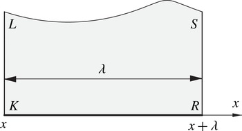
One wave period.

3. Formulae for the wave resistance in water of finite depth
Consider three physical quantities introduced by Benjamin & Lighthill (Reference Benjamin and Lighthill1954) in their development of the approximate theory of cnoidal waves. These quantities are the total head
 $R$
(the Bernoulli constant, defined by (2.2)), the volume flux
 $$\begin{eqnarray}Q=\int _{0}^{{\it\eta}(x)}v_{x}(x,y)\,\text{d}y,\end{eqnarray}$$
and the flow force
 $$\begin{eqnarray}S=\int _{0}^{{\it\eta}(x)}\left[v_{x}^{2}(x,y)+\frac{p}{{\it\rho}}\right]\text{d}y\end{eqnarray}$$
(horizontal momentum flux plus pressure force per unit span, divided by the density). In formulae (3.1), (3.2) the integration is along a vertical segment lying entirely inside the fluid.
For the goals of this section the parameter
 $S$
is of special importance. Indeed, as follows from the momentum equation, the wave drag
 $R_{w}={\it\rho}(S_{MN}-S_{KL})$
, where
 $S_{MN}$
and
 $S_{KL}$
are the parameters
 $S$
calculated for vertical segments
 $MN$
and
 $KL$
located upstream and downstream of the body, respectively (see figure 1).
Far downstream consider one wave period shown in figure 2. From the Bernoulli equation (2.2) we find that
 $$\begin{eqnarray}S=R{\it\eta}(x)-\frac{1}{2}g{\it\eta}^{2}(x)+\frac{1}{2}\int _{0}^{{\it\eta}(x)}(v_{x}^{2}-v_{y}^{2})\,\text{d}y,\end{eqnarray}$$
or
 $$\begin{eqnarray}S=R{\it\eta}(x)-\frac{1}{2}g{\it\eta}^{2}(x)+\frac{1}{2}\,\text{Im}\int _{KL}\left(\frac{\text{d}w}{\text{d}z}\right)^{2}\text{d}z,\end{eqnarray}$$
where
 $w(z)={\it\varphi}+\text{i}{\it\psi}$
is the complex potential of the wave flow, and
 $\text{d}w/\text{d}z=v_{x}-\text{i}v_{y}$
is the complex-conjugate velocity. By virtue of the
 ${\it\lambda}$
-periodicity of
 $\text{d}w/\text{d}z$
we have
 $$\begin{eqnarray}\int _{RS}z\left(\frac{\text{d}w}{\text{d}z}\right)^{2}\text{d}z+\int _{LK}z\left(\frac{\text{d}w}{\text{d}z}\right)^{2}\text{d}z={\it\lambda}\int _{KL}\left(\frac{\text{d}w}{\text{d}z}\right)^{2}\text{d}z.\end{eqnarray}$$
We integrate the analytic function
 $z(\text{d}w/\text{d}z)^{2}$
along the boundaries of the wave period in the counterclockwise direction and take the imaginary part of the result. Because on the bottom
 $\text{Im}[z(\text{d}w/\text{d}z)^{2}]=0$
, with allowance for (3.5) we get from the Cauchy theorem
 $$\begin{eqnarray}{\it\lambda}\,\text{Im}\int _{KL}\left(\frac{\text{d}w}{\text{d}z}\right)^{2}\text{d}z=\text{Im}\int _{LS}z\left(\frac{\text{d}w}{\text{d}z}\right)^{2}\text{d}z.\end{eqnarray}$$
But
 $$\begin{eqnarray}\left(\frac{\text{d}w}{\text{d}z}\right)^{2}\text{d}z=v^{2}\text{e}^{-i{\it\theta}}\,\text{d}s=v^{2}(\text{d}x-\text{i}\,\text{d}y),\end{eqnarray}$$
where
 ${\it\theta}$
is the inclination and
 $v=\sqrt{v_{x}^{2}+x_{y}^{2}}$
is the modulus of the velocity vector on the free surface
 $LS$
;
 $\text{d}s$
is a line element of
 $LS$
. Taking into account that
 $v^{2}=2(R-gy)$
, we infer that
 $$\begin{eqnarray}{\it\lambda}\,\text{Im}\!\int _{KL}\left(\frac{\text{d}w}{\text{d}z}\right)^{2}\text{d}z=\text{Im}\!\int _{LS}v^{2}(x+\text{i}y)(\,\text{d}x-\text{i}\,\text{d}y)=2\!\int _{LS}(Ry-gy^{2})\,\text{d}x-2\!\int _{LS}x(R-gy)\,\text{d}y.\end{eqnarray}$$
Integrating the second integral by parts, we obtain
 $$\begin{eqnarray}{\it\lambda}\,\text{Im}\int _{KL}\left(\frac{\text{d}w}{\text{d}z}\right)^{2}\text{d}z=2\int _{LS}\left(2Ry-\frac{3}{2}gy^{2}\right)\text{d}x-2{\it\lambda}\left[R{\it\eta}(x)-\frac{1}{2}g{\it\eta}^{2}(x)\right].\end{eqnarray}$$
From this equation and (3.4) we deduce a new representation for the flow force
 $$\begin{eqnarray}S=\frac{1}{{\it\lambda}}\int _{x}^{x+{\it\lambda}}\left[2R{\it\eta}({\it\xi})-\frac{3}{2}g{\it\eta}^{2}({\it\xi})\right]\text{d}{\it\xi},\end{eqnarray}$$
in which the integration is not along a vertical segment, as in the initial definition (3.2) of the flow force
 $S$
and in formula (1.3) by Wehausen & Laitone (Reference Wehausen, Laitone and Truesdell1960), but along one period of the free surface.
It is to be noted that this change in the line of integration is a key point in deducing formula (1.9). Indeed, because for the uniform stream
 ${\it\eta}(x)=h$
, it follows from (3.10) that
 $S_{MN}=2hR-(3/2)gh^{2}$
. But
 $R_{w}/{\it\rho}=S_{MN}-S$
, hence
 $$\begin{eqnarray}\displaystyle \frac{R_{w}}{{\it\rho}} & = & \displaystyle \frac{1}{{\it\lambda}}\int _{x}^{x+{\it\lambda}}\left(2hR-\frac{3}{2}gh^{2}-2Ry+\frac{3}{2}gy^{2}\right)\text{d}x\nonumber\\ \displaystyle & = & \displaystyle \frac{1}{{\it\lambda}}\int _{x}^{x+{\it\lambda}}\left[\frac{3}{2}g(y-h)^{2}-(2R-3gh)(y-h)\right]\text{d}x.\end{eqnarray}$$
Taking into account that
 $2R=c^{2}+2gh$
, we come to formula (1.9).
To deduce formula (1.11), which leads to
 $R_{w}=3V-2T$
for deep water, we first notice that
 $$\begin{eqnarray}V=\frac{{\it\rho}g}{2}({\it\delta}_{2}^{2}-{\it\delta}_{1}^{2}),\end{eqnarray}$$
where
 $V$
is the mean wave potential energy, defined by (1.6a
) and the lengths
 ${\it\delta}_{1}$
and
 ${\it\delta}_{2}$
are determined in (1.10). Equations (1.6), (1.9) and (3.12) yield
 $$\begin{eqnarray}R_{w}=3V+{\textstyle \frac{3}{2}}{\it\rho}g{\it\delta}_{1}^{2}+{\it\rho}(gh-c^{2}){\it\delta}_{1}.\end{eqnarray}$$
Now we express the third term in (3.13) by the mean kinetic energy
 $T$
of the waves propagating with the speed
 $c$
of the body. This
 $T$
, defined by (1.6b
), can be written as
 $$\begin{eqnarray}T=\frac{{\it\rho}}{2{\it\lambda}}\int _{x}^{x+{\it\lambda}}\,\text{d}{\it\xi}\int _{0}^{{\it\eta}(x)}[(v_{x}-c)^{2}+v_{y}^{2}]\,\text{d}y.\end{eqnarray}$$
A usual assumption (see e.g. Longuet-Higgins Reference Longuet-Higgins1975; Cokelet Reference Cokelet1977) in the theory of nonlinear periodic waves is that in the bottom-fixed reference frame the waves propagate with the velocity
 $c_{a}$
, equal to the average fluid velocity at any horizontal level completely within the fluid in the wave-fixed reference frame (in steady flow). That is
 $$\begin{eqnarray}c_{a}=\frac{1}{{\it\lambda}}\int _{x}^{x+{\it\lambda}}v_{x}({\it\xi},y)\,\text{d}{\it\xi}=\frac{C}{{\it\lambda}},\end{eqnarray}$$
where
 $$\begin{eqnarray}C={\it\varphi}(x+{\it\lambda},y)-{\it\varphi}(x,y)\end{eqnarray}$$
is the increment of the potential
 ${\it\varphi}$
in the wave (circulation in the steady motion). As was noticed by Whitham (Reference Whitham1962, p. 142) and later numerically confirmed by Salvesen & von Kerczek (Reference Salvesen and von Kerczek1976, p. 168), for the waves generated by a moving body due to nonlinear effects this assumption is not correct, i.e.
 $c\neq c_{a}$
. Taking into account this fact, we write
 $$\begin{eqnarray}T=\frac{{\it\rho}}{2}(c_{a}Q+c^{2}h_{a}-2cQ).\end{eqnarray}$$
The simplest way of deriving (3.17) is to use the formula (see Longuet-Higgins Reference Longuet-Higgins1975, p. 160)
 $$\begin{eqnarray}\mathop{\iint }_{{\it\Omega}_{z}\hspace{6.0pt}}(v_{x}^{2}+v_{y}^{2})\,\text{d}x\,\text{d}y=\mathop{\iint }_{{\it\Omega}_{w}\hspace{6.0pt}}\,\text{d}{\it\varphi}\,\text{d}{\it\psi}=CQ,\end{eqnarray}$$
where
 ${\it\varphi}$
and
 ${\it\psi}$
denote the velocity potential and stream function, and
 ${\it\Omega}_{w}$
is a domain of one period in the plane of the complex potential
 $w={\it\varphi}+\text{i}{\it\psi}$
. The formula follows from the equation
 $\partial ({\it\phi},{\it\psi})/\partial (x,y)=v_{x}^{2}+v_{y}^{2}$
and with allowance for (1.7), (3.1) its application directly leads to (3.17).
Taking into account that
 $Q=ch$
, from (3.17) we deduce
 $$\begin{eqnarray}2T={\it\rho}(cc_{a}h+c^{2}h_{a}-2c^{2}h).\end{eqnarray}$$
Let
 $c_{b}$
be the root-mean-square velocity at the bottom in steady motion:
 $$\begin{eqnarray}c_{b}^{2}=\frac{1}{{\it\lambda}}\int _{x}^{x+{\it\lambda}}v_{x}^{2}({\it\xi},0)\,\text{d}{\it\xi}.\end{eqnarray}$$
It seems that Levi-Civita (Reference Levi-Civita1925, p. 277) was the first to notice that in any periodic steady potential flow the root-mean-square velocities
 $$\begin{eqnarray}\sqrt{\frac{1}{{\it\lambda}}\int _{L}v^{2}\,\text{d}x}\end{eqnarray}$$
along one period
 $L$
of any streamline are equal. The simplest way to prove this is to integrate the analytic function
 $(\text{d}w/\text{d}z)^{2}$
along the boundaries of one period between two streamlines, and after that to use formula (3.7) and the Cauchy theorem. Taking for these two streamlines the bottom and the free surface, with allowance for the boundary condition
 $v^{2}+2g{\it\eta}(x)=2R$
we conclude
 $$\begin{eqnarray}c_{b}^{2}+2gh_{a}=2R.\end{eqnarray}$$
In unsteady motion the root-mean-square bottom velocity
 ${\it\sigma}_{b}$
is defined by (1.12). It follows from the definition (1.12) that
 ${\it\sigma}_{b}^{2}=c_{b}^{2}-2cc_{a}+c^{2}$
. Since
 $2R=c^{2}+2gh$
, we infer that
 $$\begin{eqnarray}\frac{{\it\rho}}{2}h{\it\sigma}_{b}^{2}={\it\rho}h(c^{2}-g{\it\delta}_{1}-cc_{a}).\end{eqnarray}$$
Now we sum relations (3.19) and (3.23) to get
 $$\begin{eqnarray}2T+\frac{{\it\rho}}{2}h{\it\sigma}_{b}^{2}={\it\rho}{\it\delta}_{1}(c^{2}-gh).\end{eqnarray}$$
Formula (1.11) follows from (3.13) and (3.24).
Consider now the case when the solution to the problem (2.3)–(2.6), (2.8) satisfies the conditions (2.9), i.e. we have far downstream a uniform flow with velocity
 $c_{d}$
and depth
 $h_{d}$
. For this case formula (1.9) remains correct because in deriving it we have used only the periodicity of the downstream flow. But now
 $$\begin{eqnarray}{\it\eta}(x)=h_{d},\quad h_{a}=h_{d},\quad {\it\delta}_{1}=h_{d}-h,\quad {\it\delta}_{2}^{2}={\it\delta}_{1}^{2},\end{eqnarray}$$
and formula (1.9) takes the form
 $$\begin{eqnarray}R_{w}={\it\rho}gh^{2}\frac{{\it\delta}_{1}}{h}\left(\frac{3}{2}\frac{{\it\delta}_{1}}{h}+1-\mathit{Fr}^{2}\right).\end{eqnarray}$$
It is clear that if
 ${\it\delta}_{1}=0$
, then
 $R_{w}=0$
. Let us consider the case
 ${\it\delta}_{1}\neq 0$
, i.e.
 $h_{d}\neq h$
,
 $c_{d}\neq c$
. Because the Bernoulli constant and the flow flux far upstream and far downstream are the same, we have
 $$\begin{eqnarray}ch=c_{d}h_{d},\quad c^{2}+2gh=c_{d}^{2}+2gh_{d}.\end{eqnarray}$$
If we denote
 ${\it\varkappa}=h_{d}/h$
, then
 ${\it\delta}_{1}/h={\it\varkappa}-1$
. Using (3.26) and (3.27), after some algebra we obtain the following relationships:
 $$\begin{eqnarray}R_{w}=\frac{{\it\rho}gh^{2}}{2}\frac{(1-{\it\varkappa})^{3}}{1+{\it\varkappa}},\quad {\it\varkappa}=\frac{\mathit{Fr}^{2}}{4}\left(1+\sqrt{1+\frac{8}{\mathit{Fr}^{2}}}\right),\quad \mathit{Fr}_{d}=\frac{\mathit{Fr}}{{\it\varkappa}^{3/2}}.\end{eqnarray}$$
These relationships or equivalent forms of them have appeared in a number of papers (see e.g. Binnie Reference Binnie1952; Benjamin & Lighthill Reference Benjamin and Lighthill1954; Maklakov Reference Maklakov1995; Binder et al.
Reference Binder, Vanden-Broek and Dias2009). As follows from (3.28), if the upstream Froude number
 $\mathit{Fr}<1$
, then
 ${\it\varkappa}<1$
,
 $R_{w}>0$
and the downstream Froude number
 $\mathit{Fr}_{d}>1$
. Such waveless flows, subcritical far upstream and supercritical far downstream, are called hydraulic falls or critical free-surface flows. We prefer hydraulic falls because the words ‘critical flows’ are often associated with the case when
 $c=\sqrt{gh}$
and
 $\mathit{Fr}=1$
.
Although hydraulic falls are waveless flows we shall continue to call the resistance created by them the wave resistance because, firstly, the equation for
 $R_{w}$
in (3.28) has been deduced from the general wave resistance formula (1.9). Secondly, the hydraulic falls in some range of Froude numbers are the limiting configurations of solutions with waves far downstream. We shall discuss the passage to this limit in § 6.
4. Signs of the wave resistance and upstream flow parameters
Let us assume that in the body-fixed reference frame the waves far downstream are known. This means that we know the equation of the free surface
 $y={\it\eta}(x)$
as well as all wave parameters, including the total head
 $R$
and the flow flux
 $Q$
. To determine the wave resistance
 $R_{w}$
by means of (1.9) we need to find the parameters of the upstream flow, namely the velocity
 $c$
and the undisturbed level
 $h$
. Because far upstream and far downstream we have the same
 $R$
and
 $Q$
the parameters
 $c$
and
 $h$
can be found from the system of equations (2.1), where
 $Q$
and
 $R$
are given,
 $c$
and
 $h$
are unknown.
Denote by
 $h_{c}$
and
 $h_{t}$
the heights of the crests and troughs of the waves and introduce the function
 $$\begin{eqnarray}S_{u}(c,h)={\textstyle \frac{1}{2}}h(2c^{2}+gh),\end{eqnarray}$$
where
 $S_{u}(c,h)$
is the flow force
 $S$
for a uniform stream with speed
 $c$
and depth
 $h$
.
The system (2.1) has been thoroughly investigated by Keady & Norbury (Reference Keady and Norbury1975) and Benjamin (Reference Benjamin1995). Reformulating some results of these authors in our notation we come to the following.
Proposition 1. Assume that the waves are periodic, symmetric and stationary; compute for these waves the parameters
 $Q$
,
 $R$
and
 $S$
. Then the following statements hold:
-
(i) The parameters
 $Q$
and
$R$
satisfy the inequality (4.2)Under the condition (4.2) the system (2.1) always has only two positive solutions
$$\begin{eqnarray}8R^{3}>27g^{2}Q^{2}.\end{eqnarray}$$
$c_{1},h_{1}$
and
$c_{2},h_{2}$
. For the first solution
$c_{1},h_{1}$
the upstream uniform flow is subcritical, i.e.
$c_{1}^{2}<gh_{1}$
; for the second one
$c_{2},h_{2}$
it is supercritical, i.e.
$c_{2}^{2}>gh_{2}$
. The depths
$h_{1}$
and
$h_{2}$
of the subcritical and supercritical conjugate streams satisfy the inequalities (4.3)
$$\begin{eqnarray}h_{2}<h_{t}<h_{1}<h_{c}.\end{eqnarray}$$
-
(ii) For the flow force
$S$
the following two-sided estimate is valid: (4.4)
$$\begin{eqnarray}S_{u}(c_{2},h_{2})<S<S_{u}(c_{1},h_{1}).\end{eqnarray}$$


The first statement of this proposition is a dimensional reformulation of Proposition 1R from Keady & Norbury (Reference Keady and Norbury1975) and Proposition 2 from Benjamin (Reference Benjamin1995). The left inequality in (4.4) was proved by Keady & Norbury (Reference Keady and Norbury1975, Proposition 2) and by Benjamin (Reference Benjamin1995, Proposition 3). The right inequality in (4.4) was proved by Benjamin (Reference Benjamin1995, Proposition 4), more than 40 years after the conjecture that the flow force
 $S$
satisfies the two-sided inequality (4.4) was put forward by Benjamin & Lighthill (Reference Benjamin and Lighthill1954).
Corollary to Proposition 1. Let the waves far downstream of the body satisfy the conditions of Proposition 1. For the subcritical solution
 $c=c_{1},h=h_{1}$
of the system (2.1) the line of the undisturbed level
 $y=h=h_{1}$
intersects the free surface of the waves and the wave resistance
 $R_{w}>0$
; for the supercritical solution
 $c=c_{2},h=h_{2}$
the waves lie above the undisturbed level
 $y=h=h_{2}$
and
 $R_{w}<0$
.
The statement of the corollary, concerning the location of the undisturbed levels with respect to the waves, follows from inequalities (4.3). The statement about the signs of the wave resistance
 $R_{w}$
is a consequence of the two-sided estimate (4.4), because
 $$\begin{eqnarray}R_{w}=S_{u}(c_{i},h_{i})-S,\quad i=1,2.\end{eqnarray}$$
We can conclude from the corollary that the steady free-surface flows over any obstacle which are supercritical far upstream and have a train of periodic steady waves far downstream are non-realistic, because for all of them
 $R_{w}<0$
(the wave thrust instead of wave drag). A characteristic feature of the flows with
 $R_{w}<0$
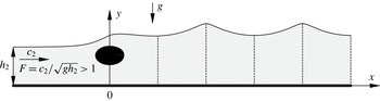
is that the waves far downstream lie above the upstream undisturbed level (see figure 3). It is to be noted that numerical evidence of existence of such flows was first demonstrated by Dias & Vanden-Broek (Reference Dias and Vanden-Broek2002, figure 7) for a bump on a horizontal bottom, and further examples have been computed by Dias & Vanden-Broek (Reference Dias and Vanden-Broek2004, figure 4), Binder et al. (Reference Binder, Vanden-Broek and Dias2009, figure 4), but the question of wave resistance has not been discussed in these works.
Sketch of a free-surface flow with a supercritical upstream Froude number.

The assertions of Proposition 1 and the above corollary relate to the case when there exist waves far downstream, i.e. the function
 ${\it\eta}_{\ast }(x)$
in (2.8) is such that
 ${\it\eta}_{\ast }(x)\not\equiv \text{const}$
. Now we formulate a proposition which includes the case
 ${\it\eta}_{\ast }(x)\equiv \text{const.}$
and connects the sign of the wave resistance with that of the defect of levels
 ${\it\delta}_{1}=h_{a}-h$
or with the sign of
 $\mathit{Fr}-1$
.
Proposition 2. Let the far-downstream waves (if they exist) be symmetric. Then the solutions to the problem (2.3)–(2.6), (2.8) possess the following properties:
-
(i)
$R_{w}>0$
iff
${\it\delta}_{1}<0$
or
$R_{w}>0$
iff
$\mathit{Fr}<1\cup {\it\delta}_{1}\neq 0$
; -
(ii)
$R_{w}<0$
iff
${\it\delta}_{1}>0$
or
$R_{w}<0$
iff
$\mathit{Fr}>1\cup {\it\delta}_{1}\neq 0$
; -
(iii)
$R_{w}=0$
iff
${\it\delta}_{1}=0$
; -
(iv) if
${\it\delta}_{1}=0$
(or
$R_{w}=0$
), then there are no waves far downstream and the upstream and downstream uniform flows are identical, i.e.
$h=h_{d}$
,
$c=c_{d}$
,
$\mathit{Fr}=\mathit{Fr}_{d}$
; -
(v) if
$\mathit{Fr}=1$
and a solution exists, then
${\it\delta}_{1}=0$
and
$R_{w}=0$
with all conclusions of statement (iv).


Proof. The proof is mainly based on the results of the above corollary and the new identity (3.24) for periodic waves. First, consider the case when there exist waves far downstream, i.e.
 ${\it\eta}_{\ast }(x)\not\equiv \text{const.}$
in (2.8). Then in the identity (3.24) the left-hand side is positive. Hence, its right-hand side
 $$\begin{eqnarray}(c^{2}-gh){\it\delta}_{1}>0.\end{eqnarray}$$
This means that the values of
 $c^{2}-gh$
and
 ${\it\delta}_{1}$
both do not vanish and their signs coincide. But according to the corollary for the wavelike solutions the wave resistance
 $R_{w}\neq 0$
and the sign of
 $c^{2}-gh$
is opposite to that of
 $R_{w}$
. This leads to the statements (i) and (ii) for the solutions with downstream waves.
Now consider the waveless solutions with
 ${\it\varkappa}=h_{d}/h\neq 1$
. From (3.28a,b
) it follows that
 $R_{w}\neq 0$
and the sign of
 $R_{w}$
is opposite to that of
 ${\it\delta}_{1}=h({\it\varkappa}-1)$
and to that of
 $\mathit{Fr}-1$
. And again we come to the statements (i) and (ii).
Thus, for the waveless solutions with
 ${\it\varkappa}=h_{d}/h\neq 1$
and the solutions with downstream waves we always have
 $R_{w}\neq 0$
,
 ${\it\delta}_{1}\neq 0$
. Therefore,
 $R_{w}$
can vanish only for the remaining case when the upstream and downstream uniform flows are identical. For this case, evidently,
 ${\it\delta}_{1}=0$
and, as follows from (3.26), the wave resistance
 $R_{w}=0$
.
The fifth statement follows from the fact that according to Proposition 1 for all flows with waves far downstream
 $\mathit{Fr}\neq 1$
. The same is true for all waveless flows with
 ${\it\varkappa}\neq 1$
, due to (3.28a,b
). The only remaining possibility is
 ${\it\varkappa}=1$
,
 $\mathit{Fr}_{d}=1$
. This reasoning finalizes the proof of the proposition.
The first statement of Proposition 2 demonstrates that for physically realistic steady free-surface flows with a positive wave resistance the defect of levels
 ${\it\delta}_{1}<0$
always exists. Now in the chain of inequalities (4.3) of Proposition 1 the mean depth
 $h_{a}$
can be included, namely
 $$\begin{eqnarray}h_{2}<h_{t}<h_{a}<h_{1}<h_{c}.\end{eqnarray}$$
From the first two statements of Proposition 2 we have the following.
Corollary to Proposition 2. Under the conditions of Proposition 2
-
(i) if
${\it\delta}<0$
, then
$\mathit{Fr}<1$
; -
(ii) if
${\it\delta}>0$
, then
$\mathit{Fr}>1$
.


The converse statements of this corollary are not true because the waveless solutions with
 ${\it\delta}=0$
,
 $\mathit{Fr}=\mathit{Fr}_{d}$
exist both for
 $\mathit{Fr}<1$
(see Forbes Reference Forbes1982; Maklakov Reference Maklakov1995; Holmes et al.
Reference Holmes, Hocking, Forbes and Baillard2013) and
 $\mathit{Fr}>1$
(see Forbes & Schwartz Reference Forbes and Schwartz1982; Vanden-Broek Reference Vanden-Broek1987). But the solutions with
 ${\it\delta}=0$
,
 $\mathit{Fr}<1$
exist only if the parameters of the disturbance are chosen by a special way.
Let us introduce the dimensionless parameter
 $$\begin{eqnarray}p=\sqrt{\frac{8R^{3}}{27g^{2}Q^{2}}}.\end{eqnarray}$$
As follows from (4.2),
 $p>1$
. The system (2.1) can be transformed to a cubic algebraic equation with respect to the squared Froude number
 $\mathit{Fr}^{2}$
(see Binnie Reference Binnie1952, (2.5)):
 $$\begin{eqnarray}(\mathit{Fr}^{2}+2)^{3}-27p^{2}\mathit{Fr}^{2}=0.\end{eqnarray}$$
To deduce (4.9) it is necessary to write (2.1) in an equivalent form:
 $$\begin{eqnarray}\frac{c^{2}}{gh}=\frac{Q^{2}}{gh^{3}},\quad \left(\frac{c^{2}}{gh}+2\right)^{3}=\frac{8R^{3}}{g^{3}h^{3}}.\end{eqnarray}$$
Dividing the second equation by the first, one gets (4.9).
It is easy to see that under the condition
 $p>1$
(4.9) always has two positive roots:
 $\mathit{Fr}^{2}<1$
and
 $\mathit{Fr}^{2}>1$
. The solutions with
 $R_{w}<0$
we consider as non-realistic and reject them. So, determining the parameters of the upstream flow from the system (2.1), we always assume that
 $c=c_{1}$
,
 $h=h_{1}$
and, hence, the Froude number
 $\mathit{Fr}=c/\sqrt{gh}<1$
.
Applying the trigonometric method to (4.9), after a little algebra we find the realistic root
 $$\begin{eqnarray}\mathit{Fr}^{2}=6p\sin [{\textstyle \frac{1}{3}}\arcsin (p^{-1})]-2<1.\end{eqnarray}$$
The second root coincides with the downstream Froude number
 $\mathit{Fr}_{d}$
for hydraulic falls and can be found from (3.28b,c
).
After finding the Froude number
 $\mathit{Fr}$
we are able to determine the upstream flow parameters
 $$\begin{eqnarray}h=\frac{1}{\mathit{Fr}^{2}+2}\frac{2R}{g},\quad c=\mathit{Fr}\sqrt{gh},\end{eqnarray}$$
which can be non-dimensionalized in any desired manner.
5. Computations of the wave resistance by a numerical method
5.1. Non-dimensionalization
In this paper we shall mainly use two types of dimensionless wave parameters. For the first type we choose
 ${\it\lambda}$
,
 $\sqrt{g{\it\lambda}}$
and
 ${\it\rho}$
as the scales for length, velocity and density, respectively. The dimensionless wave parameters, normalized by this set of scales, we denote by a bar. For example,
 $$\begin{eqnarray}\bar{h}=\frac{h}{{\it\lambda}},\quad \bar{a}=\frac{a}{{\it\lambda}},\quad \bar{c}^{2}=\frac{c^{2}}{g{\it\lambda}},\quad \bar{R}_{w}=\frac{R_{w}}{{\it\rho}g{\it\lambda}^{2}}.\end{eqnarray}$$
For the second type the quantities
 $c^{2}/g$
,
 $c$
and
 ${\it\rho}$
are chosen as the scales for length, velocity and density. The parameters normalized by these scales we denote by a hat:
 $$\begin{eqnarray}{\hat{h}}=\frac{hg}{c^{2}}=\frac{1}{\mathit{Fr}^{2}},\quad \hat{a}=\frac{ag}{c^{2}},\quad {\hat{c}}^{2}=1,\quad \hat{R}_{w}=\frac{gR_{w}}{{\it\rho}c^{4}}.\end{eqnarray}$$
The non-dimensionalization by ‘bars’ seems to be natural, but that with ‘hats’ is sometimes more useful. So, in what follows we shall use both of them and even sometimes others, as dictated by convenience.
5.2. Numerical method
For steady
 ${\it\lambda}$
-periodic waves far downstream of an obstruction the harmonic stream function
 ${\it\psi}(x,y)$
and the function
 ${\it\eta}(x)>0$
, which defines the shape of the free surface, must be
 ${\it\lambda}$
-periodic with respect to the variable
 $x$
and satisfy the boundary conditions (2.3), (2.4). It is well known that the solution to the problem (2.3), (2.4) depends on two dimensionless parameters. The main requirement for these parameters is that they should define the wave uniquely, i.e. all dimensionless wave properties are one-valued functions of these two parameters.
To calculate the wave properties we use the method of self-generating convergent meshes, suggested by Maklakov (Reference Maklakov2002). The method allows one to compute waves of any steepness with accuracy of 10–11 decimal digits.
The technique of free-point predictions, proposed in Maklakov (Reference Maklakov2002) and based on the Longuet-Higgins and Fox asymptotic theory for the almost-highest waves (see Longuet-Higgins & Fox Reference Longuet-Higgins and Fox1977, Reference Longuet-Higgins and Fox1978, Reference Longuet-Higgins and Fox1996), permits one also to determine the limiting wave properties with the same accuracy, without computing directly the highest waves.
In Maklakov (Reference Maklakov2002) to specify a wave, the parameters
 $$\begin{eqnarray}r_{0}=\exp \left(-\frac{2{\rm\pi}Q}{{\it\lambda}c_{a}}\right)\quad \text{and}\quad A=\log \frac{v_{t}}{v_{c}}\end{eqnarray}$$
have been chosen. Here
 $v_{c}$
is the velocity at the crest and
 $v_{t}$
is that at the trough of the waves in the wave-fixed frame of reference. The first parameter
 $r_{0}$
is responsible for the wave depth-to-length ratio and ranges between 0 and 1. For waves of infinite depth
 $r_{0}=0$
, for solitary waves
 $r_{0}=1$
. This parameter has been used in a number of works devoted to the nonlinear wave theory (see e.g. Schwartz Reference Schwartz1974; Cokelet Reference Cokelet1977).
The second parameter
 $A$
is responsible for the wave steepness and varies from zero to
 $+\infty$
. When
 $A=+\infty$
, the wave is of limiting height with a 120° angular crest. The values of
 $A$
close to zero correspond to infinitesimal waves. We should note that for infinitesimal waves
 $2{\rm\pi}h_{a}/{\it\lambda}=-\log \,r_{0}$
.
The high accuracy of the algorithm from Maklakov (Reference Maklakov2002) is due to the advantage of using non-uniform meshes with the location of nodes uniquely defined by the parameters
 $r_{0}$
,
 $A$
and the iteration process of self-generation. In all further computations the number of nodes distributed along a half-wavelength is taken to be equal to 2000.
After some small modification of the algorithm we are able now to specify waves by using instead of
 $r_{0}$
a more natural parameter
 $\bar{h}_{a}=h_{a}/{\it\lambda}$
(the ratio of the mean depth to wavelength). With the modified version we are able to calculate wave properties in the range
 $0.017\leqslant \bar{h}_{a}\leqslant 1000$
for any
 $A>0$
including
 $A=\infty$
. The value
 $\bar{h}_{a}=0.017$
corresponds to almost solitary waves;
 $\bar{h}_{a}=1000$
corresponds to waves on deep water.
For
 $A>5$
the asymptotic formulae of Longuet-Higgins and Fox have been used (see Longuet-Higgins & Fox Reference Longuet-Higgins and Fox1977, Reference Longuet-Higgins and Fox1978, Reference Longuet-Higgins and Fox1996; Maklakov Reference Maklakov2002). According to these formulae, for any fixed
 $\bar{h}_{a}$
or
 $r_{0}$
with increase of
 $A$
the basic wave properties (for example, the potential and kinetic energies
 $V$
and
 $T$
, impulse
 $I$
, phase velocity
 $c_{a}$
) oscillate according to the law
 $$\begin{eqnarray}{\it\omega}={\it\omega}^{\ast }+a_{{\it\omega}}e^{-3A}\cos (kA-b_{{\it\omega}})+\mathit{O}(\text{e}^{-5A}),\end{eqnarray}$$
where
 ${\it\omega}$
is a certain wave property,
 ${\it\omega}^{\ast }$
is its limit for the highest wave (in what follows we shall denote this limit by a superscript asterisk), and
 $k=2.14291\dots$
is the root of the equation
 $$\begin{eqnarray}\frac{k{\rm\pi}}{6}\tanh \frac{k{\rm\pi}}{6}=\frac{{\rm\pi}}{2\sqrt{3}},\end{eqnarray}$$
the parameters of oscillations
 ${\it\omega}^{\ast }$
,
 $a_{{\it\omega}}$
and
 $b_{{\it\omega}}$
being dependent on
 $\bar{h}_{a}$
or
 $r_{0}$
.
The only exclusion from the law (5.4) is the wave steepness
 $\bar{H}=(h_{c}-h_{t})/{\it\lambda}$
for which the asymptotic behaviour for
 $A\gg 1$
is
 $$\begin{eqnarray}\bar{H}=(1-\text{e}^{-2A})[\bar{H}^{\ast }+a_{\bar{H}}\text{e}^{-3A}\cos (kA-b_{\bar{H}})]+\mathit{O}(\text{e}^{-5A}).\end{eqnarray}$$
As was demonstrated in Maklakov (Reference Maklakov2002), the asymptotic formulae for
 $A>5$
give the wave properties with accuracy of 10–11 decimal digits, because the errors of (5.4), (5.6) are of order
 $\exp (-5A)$
.
5.3. Wave resistance as a function of geometric wave properties
Let us label a wave by specifying two geometrical parameters. The first parameter
 $\bar{h}_{a}$
, the ratio of mean depth to wavelength, varies from zero (the solitary wave) to infinity (the deep-water wave). The second parameter, the wave steepness
 $\bar{H}=2\bar{a}$
, varies from zero (the infinitesimal wave) to a limiting value
 $\bar{H}^{\ast }$
dependent on the first parameter. So,
 $$\begin{eqnarray}0\leqslant \bar{H}\leqslant \bar{H}^{\ast }(\bar{h}_{a}).\end{eqnarray}$$
But for a given
 $\bar{h}_{a}$
we are able to compute accurately the limiting value
 $H^{\ast }(\bar{h}_{a})$
, which makes it possible to normalize
 $\bar{H}$
by introducing the parameter
 ${\it\vartheta}=\bar{H}/\bar{H}^{\ast }$
, which changes in the range from zero to unity.
For finding the limiting values
 $\bar{H}^{\ast }(\bar{h}_{a})$
we present an approximate analytical formula, obtained by fitting our numerical data:
 $$\begin{eqnarray}\displaystyle \bar{H}^{\ast } & = & \displaystyle 0.1326631{\it\tau}-0.04341160{\it\tau}^{2}+0.09371880{\it\tau}^{3}\nonumber\\ \displaystyle & & \displaystyle -\,0.1986792{\it\tau}^{4}+0.5907961{\it\tau}^{5}-1.0248671{\it\tau}^{6}\nonumber\\ \displaystyle & & \displaystyle +\,0.9749535{\it\tau}^{7}-0.4831190{\it\tau}^{8}+0.09900890{\it\tau}^{9},\quad {\it\tau}=\tanh (2{\rm\pi}\bar{h}_{a}).\end{eqnarray}$$
For
 $\bar{h}_{a}\geqslant 0.017$
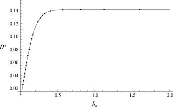
the relative error of (5.8) is not more than 0.0004 %, and its absolute error is not more than 0.00002 %. So, formula (5.8) must give an error of not more than two unities in the seventh decimal place, which is comparable with the accuracy of an exact analytical solution. The graph of the function
 $\bar{H}^{\ast }(\bar{h}_{a})$
is shown in figure 4. The points on this graph are the data from the paper by Williams (Reference Williams1981, Table 7).
The function
 $\bar{H}^{\ast }(\bar{h}_{a})$
: solid line, our computations and formula (5.8); points, the computations of Williams (Reference Williams1981).

The wave resistance
 $R_{w}$
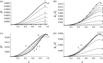
can be normalized in different ways. We have computed four wave resistance coefficients:
 $$\begin{eqnarray}\bar{R}_{w}=\frac{R_{w}}{{\it\rho}g{\it\lambda}^{2}},\quad \frac{\bar{R}_{w}}{\bar{h}_{a}^{2}}=\frac{R_{w}}{{\it\rho}gh_{a}^{2}},\quad \hat{R}_{w}=\frac{gR_{w}}{{\it\rho}c^{4}},\quad \frac{\bar{R}_{w}}{\bar{h}^{2}}=\frac{R_{w}}{{\it\rho}gh^{2}}.\end{eqnarray}$$
The graphs of these coefficients as functions of
 ${\it\vartheta}$
for different mean depth to wavelength ratio
 $\bar{h}_{a}$
are shown in figure 5. The dashed lines in the figure are plotted for
 $\bar{h}_{a}=1000$
(infinite depth case), the bold dot-dashed lines are plotted for
 $h_{a}=0.017$
(almost solitary wave case). All the graphs have been constructed parametrically by varying
 $A$
from zero to 7.5 at fixed
 $\bar{h}_{a}$
.
It is worthwhile noting that the coefficients
 $\bar{R}_{w}$
,
 $\bar{R}_{w}/\bar{h}_{a}^{2}$
and
 $\bar{R}_{w}/\bar{h}^{2}$
have a specific deficiency, namely, they tend to zero as either
 $\bar{h}_{a}\rightarrow \infty$
or
 $\bar{h}_{a}\rightarrow 0$
. For example,
 $\bar{R}_{w}$
is less than
 $5\times 10^{-6}$
at
 $\bar{h}_{a}=0.017$
for all
 ${\it\vartheta}$
. This is not the case for
 $\hat{R}_{w}=gR_{w}/({\it\rho}c^{4})$
, but as one can see in figure 5(c) for this coefficient we have the most complicated positional relationships between graphs.
Duncan (Reference Duncan1983) established that for deep water the maximum wave resistance of a two-dimensional body is
 $0.02{\it\rho}c^{4}/g$
. The dashed line in figure 5(c) confirms this conclusion, but as one can see there exist other lines in figure 5(c) which lie higher than the dashed one. This means that for water of finite depth the maximum wave resistance must be greater than
 $0.02{\it\rho}c^{4}/g$
. We have found the maximum for the wave resistance coefficient
 $\hat{R}_{w}$
by solving the maximization problem
 $$\begin{eqnarray}\hat{R}_{w}(\bar{h}_{a},A)\rightarrow \max ,\quad 0.017\leqslant \bar{h}_{a}\leqslant 1000,\quad 0\leqslant A<\infty .\end{eqnarray}$$
The results are shown in table 1, and as follows from the table,
 $R_{w}\leqslant 0.0236268{\it\rho}c^{4}/g$
which improves the estimate of Duncan (Reference Duncan1983). Table 1 presents also some properties of the waves which create the maximum wave resistance. If we choose as the basic parameter the depth
 $h$
of the upstream level, then to have the maximum resistance the body should be towed with a speed of
 $c\approx 0.692\sqrt{gh}$
, creating a wave with an amplitude of
 $0.189h$
. At these conditions the body will generate waves with wavelength
 ${\it\lambda}\approx 3h$
and defect of levels
 ${\it\delta}_{1}\approx -0.034h$
.
Graphs of four wave resistance coefficients as functions of the normalized wave steepness
 ${\it\vartheta}$
for different dimensionless mean wave depths
 $\bar{h}_{a}$
: dashed lines,
 $\bar{h}_{a}=1000$
; bold dot-dashed lines,
 $\bar{h}_{a}=0.017$
; 1–7,
 $\bar{h}_{a}=0.05,0.1,0.15,0.2,0.3,0.5,1.0$
.

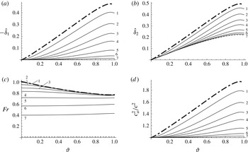
Graphs of the parameters
 $\hat{{\it\delta}}_{1}={\it\delta}_{1}g/c^{2}$
,
 $\hat{{\it\delta}}_{2}={\it\delta}_{2}g/c^{2}$
,
 $\mathit{Fr}$
and
 $c_{a}^{2}/c^{2}$
as functions of
 ${\it\vartheta}$
for different
 $\bar{h}_{a}$
: dashed lines,
 $\bar{h}_{a}=1000$
; bold dot-dashed lines,
 $\bar{h}_{a}=0.017$
; 1–7,
 $\bar{h}_{a}=0.05,0.1,0.15,0.2,0.3,0.5,1.0$
.

Maximum wave resistance coefficient
 $\hat{R}_{w}=gR_{w}/({\it\rho}c^{4})$
and the corresponding wave properties.

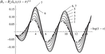
Reconstruction of all graphs of figure 5(c), which allows one to see the oscillations: dashed line,
 $\bar{h}_{a}=1000$
; bold dot-dashed line,
 $\bar{h}_{a}=0.017$
; 1–7,
 $\bar{h}_{a}=0.05,0.1,0.15,0.2,0.3,0.5,1.0$
. The dashed line almost coincides with lines 6,7.

As one can see in figure 5(b,d), at the same
 ${\it\vartheta}$
the values of the wave resistance
 $\bar{R}_{w}/\bar{h}_{a}^{2}$
are almost twice those of
 $\bar{R}_{w}/\bar{h}^{2}$
. The reason is just in the defect of levels
 ${\it\delta}_{1}=h_{a}-h<0$
. To elucidate the intricate location of the graphs in figure 5(c) and to see explicitly how this defect can be large, consider formula (1.9) for the waves resistance. Its dimensionless analogue is
 $$\begin{eqnarray}\hat{R}_{w}=\frac{gR_{w}}{{\it\rho}c^{4}}=\frac{3}{2}\hat{{\it\delta}}_{2}^{2}+\left(\frac{1}{\mathit{Fr}^{2}}-1\right)\hat{{\it\delta}}_{1}.\end{eqnarray}$$
So,
 $\hat{R}_{w}$
depends on three parameters: the dimensionless defect of levels,
 $\hat{{\it\delta}}_{1}={\it\delta}_{1}g/c^{2}$
, the dimensionless root-mean-square deviation of the free-surface shape far downstream from the undisturbed level,
 $\hat{{\it\delta}}_{2}={\it\delta}_{2}g/c^{2}$
and the Froude number,
 $\mathit{Fr}$
. The graphs of these three parameters as functions of
 ${\it\vartheta}$
for different
 $\bar{h}_{a}$
are shown in figure 6(a–c). All three plots demonstrate a similar behaviour: the parameters monotonically increase as
 $\bar{h}_{a}$
decreases. Moreover, for shallow waves they achieve significant values which are several tens of times greater than
 $\hat{R}_{w}$
, but the summation of two terms of different signs in (5.11) leads to rather small values of
 $\hat{R}_{w}$
and the intricate location of the graphs in figure 5(c).
In figure 6(d) we show the ratio of the squared velocity
 $c_{a}$
, defined by (3.15), to the squared speed of the body
 $c$
. As has been already mentioned in § 3 the velocity
 $c_{a}$
is usually assumed to be the velocity of travelling waves propagating above an immobile bottom (Longuet-Higgins Reference Longuet-Higgins1975; Cokelet Reference Cokelet1977). For shallow waves the ratio again achieves significant values and always
 $c_{a}>c$
.
In closing this subsection it should be noted that all graphs in figures 5, 6 oscillate as
 ${\it\vartheta}\rightarrow 1$
, i.e. the graphs have an infinite set of maxima and minima in the vicinity of
 ${\it\vartheta}=1$
. To see these oscillations, the graphs should be reconstructed. Indeed, according to the laws (5.4), (5.6) the oscillation will be seen if we put along the abscissa axis the values
 $-\log (1-{\it\vartheta})$
and along the ordinate axis the values
 $[{\it\omega}-{\it\omega}^{\ast }(\bar{h}_{a})](1-{\it\vartheta})^{-3/2}$
, where
 ${\it\omega}$
is an oscillating wave property. As an example we have reconstructed in this way all graphs of figure 5(c). The results are shown in figure 7, and as one can see the graphs demonstrate more regular behaviour than those of 5(c).
A free-surface flow close to a hydraulic fall.

6. Further analysis of the results and discussion
6.1. On the passage of steady free-surface flows with downstream waves to the limit of hydraulic falls
Miles (Reference Miles1986), Naghdi & Vongsarnpigoon (Reference Naghdi and Vongsarnpigoon1986) and Shen & Shen (Reference Shen and Shen1990), by means of different but similar shallow-water theories, established that for subcritical streams the train of cnoidal waves behind an obstruction for some relationships between the parameters defining the flow can degenerate to a so-called hydraulic fall, i.e. a waveless flow which is subcritical upstream and supercritical downstream. A schematic of the flow close to a hydraulic fall is shown in figure 8.
Forbes (Reference Forbes1988), by making use of a boundary-integral technique for satisfying exactly nonlinear boundary conditions on the free surface, computed numerically hydraulic falls over a semi-circular obstruction. He demonstrated that for a semi-circle of any radius less than the depth of the channel a hydraulic fall solution can be obtained by choosing the velocity of the incident flow, and so choosing the upstream Froude number
 $\mathit{Fr}<1$
. Dias & Vanden-Broek (Reference Dias and Vanden-Broek1989) came to the same conclusion for a triangular obstacle.
In studying subcritical free-surface flows over a semi-circular obstruction, Forbes & Schwartz (Reference Forbes and Schwartz1982) conjectured that:
-
(i) solutions possessing waves might also be possible in the approximate interval of the Froude numbers
$1<\mathit{Fr}<1.3$
; and -
(ii) as
$\mathit{Fr}$
increased, the wavelength of the downstream waves would increase, ultimately giving a downstream solitary wave at about
$\mathit{Fr}\approx 1.3$
.


The second part of this conjecture is correct in the sense that with increase of the upstream Froude number
 $\mathit{Fr}$
the downstream wave train can degenerate to a downstream solitary wave (see figure 8), but is not correct concerning
 $\mathit{Fr}\approx 1.3$
. It is to be noted that Forbes (Reference Forbes1988), on the basis of the results by Vanden-Broek (Reference Vanden-Broek1987), had already doubted the validity of the above conjecture.
Maklakov (Reference Maklakov1995), investigating the flow over a line vortex by an integral equation method, has numerically proved that the downstream steady wave train can degenerate to a solitary wave in the range of the upstream Froude numbers of approximately [0.761, 1). This result is not in contradiction to that of § 4, where we have rigorously proved that the realistic (with
 $R_{w}>0$
) steady free-surface flows over any obstruction are subcritical, but is in contradiction with the first part of the conjecture by Forbes & Schwartz (Reference Forbes and Schwartz1982), which seemed to be based on the fact that for solitary waves the Froude number is approximately in the range
 $1<\mathit{Fr}<1.3$
.
The explanation of the contradiction is rather simple: here we are talking about different Froude numbers. Indeed, consider a body, for instance a bump on the bottom, that generates a wave train of very long waves, as shown in figure 8. The left side of this flow is just a hydraulic fall. The upstream Froude number
 $\mathit{Fr}=c/\sqrt{gh}=c_{1}/\sqrt{gh_{1}}<1$
is one of two real roots of equation (4.9), and
 $c=c_{1}$
and
 $h=h_{1}$
is a subcritical solution to system (2.1) (see Proposition 1 of § 4). The supercritical solution of the system (2.1) is
 $c=c_{2}$
and
 $h=h_{2}$
. But for hydraulic falls
 $c_{2}=c_{d}$
and
 $h_{2}=h_{d}$
, and therefore, the downstream Froude number
 $\mathit{Fr}_{d}=c_{d}/\sqrt{gh_{d}}>1$
is the second real root of equation (4.9).
So,
 $\mathit{Fr}=c/\sqrt{gh}$
is an upstream definition of the Froude number
 $\mathit{Fr}$
for a downstream solitary wave. A usual definition of the Froude number for solitary waves is
 $\mathit{Fr}_{d}=c_{d}/\sqrt{gh_{d}}$
, and this definition is connected with that of the upstream Froude number
 $\mathit{Fr}$
by (3.28b,c
). If we put in these equations the bounds of the interval [0.761, 1), we get the interval (1, 1.294]. It is important to note that for solitary waves the maximum Froude number is
 $\sqrt{1.67498}=1.29421$
(see Tanaka Reference Tanaka1986, table 2). So, the approximate value 1.294 is in good agreement with that of Tanaka (Reference Tanaka1986).
In the next subsection we refine the range of the upstream Froude number in which the train of non-breaking long waves can degenerate to a solitary wave. Now we should notice that the range
 $0.761\leqslant \mathit{Fr}<1$
is in contradiction with the experiments for hydraulic falls carried out by Forbes (Reference Forbes1988). In these experiments
 ${\it\varkappa}$
ranges approximately from 0.05 to 0.45 (see Forbes Reference Forbes1988, figure 5). For hydraulic falls, as follows from (3.28b
),
 $$\begin{eqnarray}\mathit{Fr}^{2}=\frac{2{\it\varkappa}^{2}}{{\it\varkappa}+1}.\end{eqnarray}$$
Then, we infer from (3.28b,c
), (6.1) that in the experiments the upstream and downstream Froude numbers are in the ranges of
 $0.07\leqslant \mathit{Fr}\leqslant 0.53$
and of
 $1.75\leqslant \mathit{Fr}_{d}\leqslant 6.12$
, respectively. But in the latter interval steady non-breaking solitary waves simply do not exist.
It is worth noting that in the experiments by Forbes (Reference Forbes1988) as well as in the analogous experiments by Sivakumaran, Tingsanchali & Hosking (Reference Sivakumaran, Tingsanchali and Hosking1983) the levels
 $h$
and
 $h_{d}$
were not fixed, but measured, depending on the volume discharge
 $Q$
which could be varied. Apparently, in the experiments the steady hydraulic falls were obtained by the process of self-stabilization of initially unsteady flows. Possibly, this self-stabilization takes place only if the volume discharge
 $Q$
is small enough, and the corresponding Froude number
 $\mathit{Fr}<\mathit{Fr}_{\mathit{crit}}<0.761$
. This reasoning poses an interesting question of finding a theoretical value of
 $\mathit{Fr}_{\mathit{crit}}$
by investigating the stability of hydraulic falls.
6.2. Analytical representation of the maximum wave resistance coefficient for trains of long waves
In this subsection we return to the method of specifying waves by the parameters
 $r_{0}$
and
 $A$
with a small difference, namely, instead of
 $r_{0}$
we choose
 $$\begin{eqnarray}\mathit{Fr}_{l}=\sqrt{\frac{\tanh (\log r_{0})}{\log r_{0}}}=\sqrt{-\frac{1}{\log r_{0}}\frac{1-r_{0}^{2}}{1+r_{0}^{2}}}.\end{eqnarray}$$
As well as
 $r_{0}$
, the parameter
 $\mathit{Fr}_{l}$
also changes from zero to unity, and again zero corresponds to infinite depth waves, and unity corresponds to solitary waves. The convenience of
 $\mathit{Fr}_{l}$
is that for infinitesimal waves
 $\mathit{Fr}_{l}=\mathit{Fr}$
, where
 $\mathit{Fr}$
is the Froude number. So, the deviation of
 $\mathit{Fr}$
from
 $\mathit{Fr}_{l}$
shows the influence of nonlinear effects. At a given
 $\mathit{Fr}_{l}\in [0,1]$
(6.2) is a nonlinear equation with respect to
 $r_{0}$
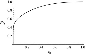
which always has a unique solution that has to be found numerically. The graph of the function
 $\mathit{Fr}_{l}(r_{0})$
is plotted in figure 9.
The graph of the function
 $\mathit{Fr}_{l}(r_{0})$
.

In figure 10 the solid lines demonstrate the parametric relationships between the wave resistance coefficient
 $gR_{w}/({\it\rho}c^{4})=\hat{R}_{w}(A)$
and the Froude number
 $\mathit{Fr}(A)$
at fixed
 $\mathit{Fr}_{l}=\text{const}$
. The parameters
 $A$
and
 $\mathit{Fr}_{l}$
vary within the ranges
 $$\begin{eqnarray}0\leqslant A\leqslant 7.5,\quad 0.01\leqslant \mathit{Fr}_{l}\leqslant \mathit{Fr}_{l\,\mathit{max}}=0.9981563392408.\end{eqnarray}$$
The value
 $A=7.5$
corresponds to almost highest waves, the value
 $\mathit{Fr}_{l}=\mathit{Fr}_{l\,\mathit{max}}$
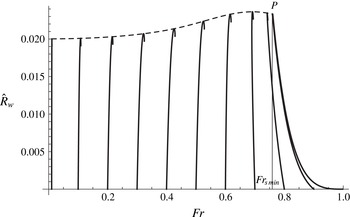
corresponds to almost solitary waves. The dashed line shows the maxima of the wave drag coefficients
 $\hat{R}_{w}$
for fixed Froude numbers
 $\mathit{Fr}\leqslant \mathit{Fr}_{s\,\mathit{min}}=0.760706$
. This curve has an explicit maximum as already mentioned in table 1.
Solid lines are the parametric relationships between the wave resistance coefficient
 $gR_{w}/({\it\rho}c^{4})=\hat{R}_{w}(A)$
and the Froude number
 $\mathit{Fr}(A)$
for fixed
 $\mathit{Fr}_{l}=\text{const}$
. The left-hand line is at
 $\mathit{Fr}_{l}=0.01$
, the right-hand line is at
 $\mathit{Fr}_{l}=\mathit{Fr}_{l\,\mathit{max}}=0.9981563392408$
(
 $r_{0}=0.9$
). The dashed line is an envelope of the solid lines.

In figure 10 the dashed line intersects the right-hand solid line at a point
 $P$
whose abscissa is
 $\mathit{Fr}_{s\,\mathit{min}}$
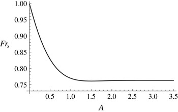
. The accurate value
 $\mathit{Fr}_{s\,\mathit{min}}=0.760706$
has been determined by finding a minimum of the function
 $\mathit{Fr}=\mathit{Fr}_{s}(A)$
, that is the dependence between the upstream Froude number
 $\mathit{Fr}$
and the parameter
 $A$
at
 $\mathit{Fr}_{l}=\mathit{Fr}_{l\,\mathit{max}}$
. The value
 $\mathit{Fr}_{l}=\mathit{Fr}_{l\,\mathit{max}}=0.9981563392408$
exactly corresponds to
 $r_{0}=0.9$
in (6.2). As was noticed in Maklakov (Reference Maklakov2002, p. 88) the long waves at
 $r_{0}=0.9$
have an almost uniform velocity distribution under the trough and approximate the properties of solitary waves up to 11 decimal places of precision. So, the function
 $\mathit{Fr}=\mathit{Fr}_{s}(A)$
represents the dependence between the Froude number
 $\mathit{Fr}$
and the parameter
 $A$
for solitary waves. The graph of this function is shown in figure 11.
The dependence
 $\mathit{Fr}=\mathit{Fr}_{s}(A)$
for solitary waves (
 $r_{0}=0.9$
) between the upstream Froude number
 $\mathit{Fr}$
and the parameter
 $A$
.

The function
 $\mathit{Fr}=\mathit{Fr}_{s}(A)$
oscillates by the law (5.4), and according to our calculations the parameters of oscillations are as follows:
 $$\begin{eqnarray}\mathit{Fr}_{s}(A)=\mathit{Fr}_{s}^{\ast }+0.3471e^{-3A}\cos (kA-1.0428),\quad \mathit{Fr}_{s}^{\ast }=0.7629045094,\end{eqnarray}$$
where
 $\mathit{Fr}_{s}^{\ast }=\mathit{Fr}_{s}(\infty )$
is the upstream Froude number for the highest solitary wave. If we put this
 $\mathit{Fr}_{s}^{\ast }$
in (3.28b,c
), we get
 $\mathit{Fr}_{d}=1.2908904559$
, which is in excellent agreement with the value 1.2908904558, obtained by Maklakov (Reference Maklakov1995) for the Froude number of the solitary wave of maximum height.
Thus, in figure 10 the dashed line (
 $0<\mathit{Fr}\leqslant \mathit{Fr}_{s\,\mathit{min}}$
) shows the maximum wave resistance coefficients
 $\hat{R}_{w}$
at fixed Froude numbers
 $\mathit{Fr}$
, and these maxima are created by waves of finite length. The right-hand solid line of the figure (
 $\mathit{Fr}_{s\,\mathit{min}}\leqslant \mathit{Fr}<1$
) does the same, but the maxima are created by solitary waves.
The right-hand solid line in figure 10 is of special interest, because, on the one hand, it shows the dependence between
 $\mathit{Fr}$
and
 $\hat{R}_{w\,\mathit{max}}$
, and on the other hand, this dependence is for hydraulic falls (wavelengths
 ${\it\lambda}\rightarrow \infty$
). But as
 ${\it\lambda}\rightarrow \infty$
the function
 $R_{w}(\mathit{Fr})$
can be found analytically from (3.28a,b
). Taking into account (3.28a,b
), after a little algebra we arrive at the formula
 $$\begin{eqnarray}R_{w\,\mathit{max}}={\it\rho}gh^{2}~D(\mathit{Fr}),\quad D(\mathit{Fr})={\textstyle \frac{1}{2}}[1+{\textstyle \frac{5}{2}}\mathit{Fr}^{2}-{\textstyle \frac{1}{8}}\mathit{Fr}^{4}-{\textstyle \frac{1}{8}}\mathit{Fr}(8+\mathit{Fr}^{2})^{3/2}],\end{eqnarray}$$
which exactly coincides with that derived by Benjamin & Lighthill (Reference Benjamin and Lighthill1954, p. 455) for the maximum wave resistance of long waves. Thus, the formula
 $$\begin{eqnarray}\hat{R}_{w\,\mathit{max}}=\frac{1}{\mathit{Fr}^{4}}D(\mathit{Fr})\end{eqnarray}$$
expresses analytically the maximum wave resistance coefficient
 $\hat{R}_{w}$
in the range of the Froude numbers
 $$\begin{eqnarray}0.760706\leqslant \mathit{Fr}<1\end{eqnarray}$$
for steady non-breaking waves, generated by a body or a bump on the bottom. At the same time this formula expresses the resistance coefficient
 $\hat{R}_{w}$
for hydraulic falls in a wider range, namely,
 $\mathit{Fr}\in (0,1)$
.
By means of (6.6) we can check our assertion that the waves at
 $\mathit{Fr}_{l}=\mathit{Fr}_{l\,\mathit{max}}$
approximate the properties of solitary waves up to 11 decimal places of precision. We have chosen several values of
 $A$
, then we have calculated numerically at
 $\mathit{Fr}_{l}=\mathit{Fr}_{l\,\mathit{max}}$
the corresponding values of
 $\mathit{Fr}$
and
 $\hat{R}_{w}$
, and inserting the obtained
 $\mathit{Fr}$
into (6.6), we have found
 $\hat{R}_{w}$
analytically. The results are in table 2 and they confirm the assertion.
Comparison of numerical computations of the wave resistance coefficient
 $\hat{R}_{w}$
with the analytical formula (6.6).

The value
 $\mathit{Fr}_{\mathit{min}}=0.760706$
is a minimum upstream Froude number at which a downstream solitary wave exists. So the passage of steady non-breaking waves to the limit of hydraulic falls is only possible in the range (6.7). The corresponding range of downstream Froude numbers obtained by means of (3.28b,c
) is
 $$\begin{eqnarray}1<\mathit{Fr}_{d}\leqslant 1.29421,\end{eqnarray}$$
which again is in a full agreement with the computations by Tanaka (Reference Tanaka1986, table 2).
6.3. Wave resistance in deep water
As already mentioned in the introduction to the paper, our formula (1.13) for the wave resistance in deep water follows from formula (1.4) of Duncan (Reference Duncan1983). Besides (1.4), Duncan has deduced two more analytical formulae, which express the wave resistance coefficients
 $\bar{R}_{w}$
and
 $\hat{R}_{w}$
in terms of the wave amplitude:
 $$\begin{eqnarray}(2{\rm\pi})^{2}\bar{R}_{w}=\frac{(2{\rm\pi})^{2}R_{w}}{{\it\rho}g{\it\lambda}^{2}}=\frac{1}{4}{\it\alpha}^{2}-\frac{3}{8}{\it\alpha}^{4},\quad \hat{R}_{w}=\frac{gR_{w}}{{\it\rho}c^{4}}=\frac{1}{4}{\it\alpha}^{2}-\frac{7}{8}{\it\alpha}^{4},\quad {\it\alpha}=\frac{2{\rm\pi}a}{{\it\lambda}}={\rm\pi}\bar{H}.\end{eqnarray}$$
Formulae (6.9), which have been obtained by making use of the third-order Stokes wave theory, contain terms up to the fourth order in
 $a$
. By means of (1.13) we are able to extend the Duncan results up to the eighth order in
 $a$
. Indeed, Longuet-Higgins (Reference Longuet-Higgins1975) on the basis of the results of Schwartz (Reference Schwartz1974) established that
 $$\begin{eqnarray}\frac{(2{\rm\pi})^{2}T}{{\it\rho}g{\it\lambda}^{2}}=\frac{1}{4}{\it\alpha}^{2}-\frac{19}{48}{\it\alpha}^{6}-\frac{3317}{2880}{\it\alpha}^{8},\quad \frac{(2{\rm\pi})^{2}V}{{\it\rho}g{\it\lambda}^{2}}=\frac{1}{4}{\it\alpha}^{2}-\frac{1}{8}{\it\alpha}^{4}-\frac{19}{48}{\it\alpha}^{6}-\frac{3077}{2880}{\it\alpha}^{8},\end{eqnarray}$$
 $$\begin{eqnarray}\frac{2{\rm\pi}c^{2}}{g{\it\lambda}}=1+{\it\alpha}^{2}+\frac{1}{2}{\it\alpha}^{4}+\frac{1}{4}{\it\alpha}^{6}-\frac{22}{45}{\it\alpha}^{8}.\end{eqnarray}$$
Using
 $R_{w}=3V-2T$
and taking into account that
 $\hat{R}_{w}=\bar{R}_{w}/\bar{c}^{4}$
, we get
 $$\begin{eqnarray}(2{\rm\pi})^{2}\bar{R}_{w}=\frac{{\it\alpha}^{2}}{4}-\frac{3{\it\alpha}^{4}}{8}-\frac{19{\it\alpha}^{6}}{48}-\frac{2597{\it\alpha}^{8}}{2880},\quad \hat{R}_{w}=\frac{{\it\alpha}^{2}}{4}-\frac{7{\it\alpha}^{4}}{8}+\frac{41{\it\alpha}^{6}}{48}-\frac{3557{\it\alpha}^{8}}{2880}.\end{eqnarray}$$
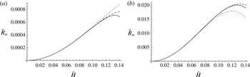
In figure 12 the graphs of the wave resistance coefficients
 $\bar{R}_{w}$
and
 $\hat{R}_{w}$
as functions of the wave steepness
 $\bar{H}=H/{\it\lambda}=2a/{\it\lambda}$
are shown. The graphs demonstrate that the increase of the number of terms in the expansions for the coefficients leads to a rather significant improvement of accuracy.


7. Conclusions
The wave resistance is an important parameter of free-surface flows, which is difficult to compute, especially for nonlinear problems. A standard method of finding it by integrating the pressure distribution along a body surface can lead to rather unexpected results. The problem is that this parameter is small and due to numerical errors it is easy to get, for example, a wave thrust instead of drag. In § 3 of this paper we have deduced formula (1.9), which seems to be more effective than the standard integration. Indeed, the formula contains only two unknown geometric parameters
 ${\it\delta}_{1}$
and
 ${\it\delta}_{2}$
, which are, respectively, the mean and root-mean-square deviations of the free-surface shape far downstream from the undisturbed level. In solving free-surface problems by any method, accurate or approximate, analytical or numerical, finding the free-surface shape is a necessary element, but with knowledge of this element the parameters
 ${\it\delta}_{1}$
and
 ${\it\delta}_{2}$
can be easily computed, and hence the wave resistance will be found.
In § 4 we have analysed the relationships between the parameters of the upstream flow and the downstream waves. Here the results by Keady & Norbury (Reference Keady and Norbury1975) and Benjamin (Reference Benjamin1995) have turned out to be very helpful. Making use of some of their results, we have rigorously proved that realistic steady free-surface flows with a positive wave resistance exist only if the upstream flow is subcritical, i.e. the Froude number
 $\mathit{Fr}=c/\sqrt{gh}<1$
. For all solutions with downstream waves obtained by a perturbation of a supercritical upstream uniform flow the wave resistance is negative. In that section we have also deduced explicit analytical formulae, which express the parameters of the upstream flow in terms of those of the downstream waves.
In fact, in §§ 3 and 4 we have introduced some new useful physical properties inherent to a system of steady periodic waves. Among them the most important are the speed
 $c$
and depth
 $h$
of a uniform stream which without dissipation is able to create this system due to some disturbance located in the stream. For example, by using (4.11) we are able to calculate the Froude number for any system of periodic steady waves which can be generated by a moving body. Most interesting is that this Froude number is always less than unity, including the case of solitary waves (else the wave resistance will be negative), which, generally, confirms the conclusions of the linear wave theory. In the set of these useful properties the wave resistance, of course, is included.
Section 5 was devoted to numerical computations. By the method of Maklakov (Reference Maklakov2002) we have calculated accurate values of the wave resistance depending on the wavelength, amplitude and average depth. So, we demonstrate that the wave resistance is a function of geometric wave properties.
In § 6 we have investigated the possibility of the passage of free-surface flows with downstream non-breaking waves to the limit of hydraulic falls. We have demonstrated that this passage is only possible if the upstream Froude number
 $\mathit{Fr}$
is in the range
 $0.760706\leqslant \mathit{Fr}<1$
.
Nonlinear steady periodic waves, as well as free-surface flows over any obstruction, can be computed by any method, accurate or approximate, analytical or numerical. So far we have determined the wave resistance by the parameters of generated waves only numerically. But the above investigations make it possible to deduce analytical formulae which connect the wave resistance with the amplitude and depth of the waves. This can be done, for example, by the Stokes method. In particular, in the last subsection of § 6 we have demonstrated such a possibility for the waves in deep water, where formulae (1.2) by Kelvin (1887) and (1.8) by Duncan (Reference Duncan1983) have been extended up to the eighth order in wave amplitude. Obtaining analogous results for waves on water of finite depth will be a subject of our further investigations.
Acknowledgements
The work was supported by the Russian Science Foundation, project no. 14-19-01633. The authors are very grateful to the referees for valuable comments which were very constructive and allowed us to improve the manuscript substantially.