1 Introduction
When a shockwave propagates along a magnetic field
 $\boldsymbol{B}_{0}$
, magnetohydrodynamics (MHD) states that the fluid is disconnected from the field (Lichnerowicz Reference Lichnerowicz1976; Majorana & Anile Reference Majorana and Anile1987). As a result, the density jump at the front does not depend on
 $B_{0}$
. However, recent particle-in-cell (PIC) simulations of such parallel relativistic shocks in collisionless pair plasmas found that, with increasing
 $B_{0}$
, the density jump becomes progressively smaller than the MHD prediction (Bret et al.
Reference Bret, Pe’er, Sironi, SaḐowski and Narayan2017). This behaviour could be traced to the inability of the downstream plasma to efficiently isotropize the particle distribution, as the field tends to guide particles and generate an anisotropic distribution function (Bret Reference Bret2016).
Regardless of whether the system is relativistic or not, one expects the plasma to display a one-dimensional (1-D) behaviour in the limit of infinite field strength. For example, the density jump for a non-relativistic strong shock in this limit should tend to
 $(\unicode[STIX]{x1D6E4}_{1D}+1)/(\unicode[STIX]{x1D6E4}_{1D}-1)=2$
, with the adiabatic index of a 1-D gas
 $\unicode[STIX]{x1D6E4}_{1D}=3$
.
Some authors have already dealt with anisotropic distributions in magnetized shocks, which eventually result in anisotropic pressures (Karimabadi, Krauss-Varban & Omidi Reference Karimabadi, Krauss-Varban and Omidi1995; Vogl et al. Reference Vogl, Biernat, Erkaev, Farrugia and Mühlbachler2001). In this respect, Erkaev, Vogl & Biernat (Reference Erkaev, Vogl and Biernat2000) and Vogl et al. (Reference Vogl, Biernat, Erkaev, Farrugia and Mühlbachler2001) studied the jump conditions for non-relativistic perpendicular and oblique shocks, while Gerbig & Schlickeiser (Reference Gerbig and Schlickeiser2011) computed the jump conditions for relativistic MHD shocks in a gyrotropic plasma.
The following sentences from Erkaev et al. (Reference Erkaev, Vogl and Biernat2000) describe well a common feature of many such studies: ‘the ratio of the perpendicular and parallel plasma pressures downstream of the shock is an unknown parameter that has to be determined. In principle, this parameter depends on the structure of the shock; however, this is beyond the scope of an MHD model’. That is, MHD per se cannot predict the anisotropy. Still, PIC simulations like the ones conducted in Bret et al. (Reference Bret, Pe’er, Sironi, SaḐowski and Narayan2017) in the relativistic regime, show a deterministic downstream anisotropy in terms of the initial parameters of the problem.
The novelty of the present work is that, while we work within an MHD formalism, we do not treat the downstream anisotropy as a free parameter which would merely be constrained by some instability thresholds. Rather, we compute the anisotropy by assuming a certain kinetic history of the plasma through the shock front. In spirit, our work is somewhat similar to Vogl et al. (Reference Vogl, Biernat, Erkaev, Farrugia and Mühlbachler2001), who also solved for the anisotropy in the post-shock plasma. Their work focused on the mirror instability, which is relevant for their perpendicular and oblique shocks, whereas we consider the firehose instability, which is relevant for our parallel shocks. In addition, as we explain below, we find that it is necessary to consider the problem as a two-stage process (Stage 1, Stage 2), but Vogl et al. (Reference Vogl, Biernat, Erkaev, Farrugia and Mühlbachler2001) ignore this complication.
A conundrum in this respect is the following. While in the absence of a magnetic field the Vlasov equation predicts that anisotropic distributions are unstable (Weibel Reference Weibel1959), it does not impose a unique degree of anisotropy in the presence of a field. Proofs of this are the beautiful studies of the solar wind, which show that the parallel and perpendicular temperatures, while limited by the thresholds for mirror and firehose instabilities, populate all regions of the stable zone (Bale et al. Reference Bale, Kasper, Howes, Quataert, Salem and Sundkvist2009; Maruca, Kasper & Bale Reference Maruca, Kasper and Bale2011; Schlickeiser et al. Reference Schlickeiser, Michno, Ibscher, Lazar and Skoda2011). As a result, a full range of anisotropy degrees can be found in the solar wind, all of them stable.Footnote 1
In the context of shock physics, one might expect the downstream anisotropy to be a function of the field strength and of the upstream properties (Bret et al. Reference Bret, Pe’er, Sironi, SaḐowski and Narayan2017). A determination of this functional dependence would allow for a modification of MHD codes, making them capable of mimicking the effects of the underlying kinetic dynamics.
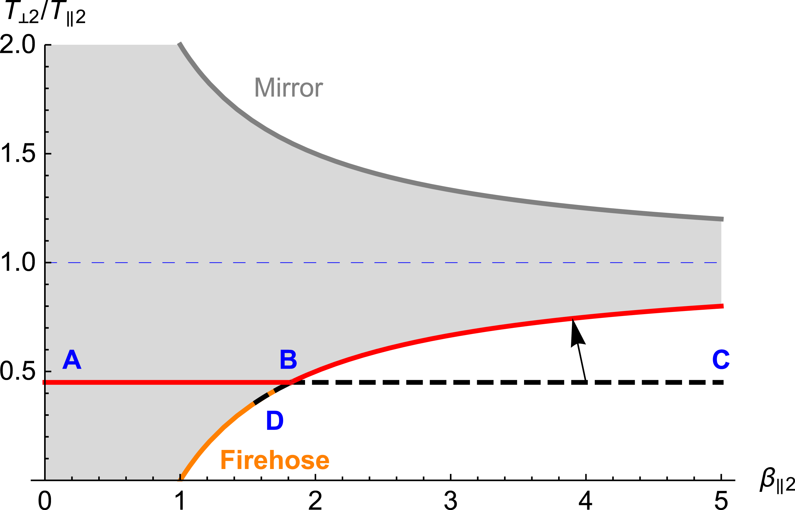
When the plasma arrives downstream (subscripts ‘2’), it comes with a certain anisotropy constrained by the condition
 $T_{\bot 2}=T_{\bot 1}$
, and a certain
 $\unicode[STIX]{x1D6FD}_{\Vert 2}$
parameter. As explained in the text (see (i)–(iv) after (1.2)), our scenario implies
 $T_{\bot 2}/T_{\Vert 2}<1$
(the line ABC for the case considered here). If
 $\unicode[STIX]{x1D6FD}_{\Vert 2}$
is such that the plasma lies inside the firehose stable region (grey shaded region, segment AB), then it remains as it is. But if the plasma arrives in an unstable region of the phase space (segment BC), it will move to a point on the firehose threshold (arrow). Thus, the end state of the plasma is somewhere on the red line. The short dashed line on the firehose threshold curve, between B and D, is explained in § 5.

As a first step towards an understanding of this problem, we present a scenario for the history of the plasma through the shock front. Consider figure 1 which shows the downstream phase space
 $(\unicode[STIX]{x1D6FD}_{\Vert 2},~T_{\bot 2}/T_{\Vert 2})$
, with
 $$\begin{eqnarray}\unicode[STIX]{x1D6FD}_{\Vert 2}=\frac{n_{2}k_{B}T_{\Vert 2}}{B_{0}^{2}/8\unicode[STIX]{x03C0}},\end{eqnarray}$$
where the subscript ‘2’ stands for the downstream properties (‘1’ stands for the upstream), ‘
 $\Vert ,\bot$
’ refer to ‘parallel’ and ‘perpendicular’ to the field respectively, and
 $k_{B}$
is the Boltzmann constant. The field
 $\boldsymbol{B}_{0}$
is aligned with the
 $x$
axis, which is also the direction of the flow, i.e. we consider parallel (non-relativistic) shocks.
In the region
 $T_{\bot 2}/T_{\Vert 2}<1$
, the stability of the plasma is limited by the firehose instability threshold (Gary Reference Gary1993),
 $$\begin{eqnarray}\frac{T_{\bot 2}}{T_{\Vert 2}}=1-\frac{1}{\unicode[STIX]{x1D6FD}_{\Vert 2}},\end{eqnarray}$$
while in the region
 $T_{\bot 2}/T_{\Vert 2}>1$
, it is limited by the mirror instability threshold,
 $T_{\bot 2}/T_{\Vert 2}=1+1/\unicode[STIX]{x1D6FD}_{\Vert 2}$
. As discussed below, the latter is not of interest for the problem considered in this paper.
Proposed scenario for the plasma, from the upstream to the downstream. The upstream plasma is isotropic. Then, across the shock front, we assume that
 $T_{\bot }$
is conserved. This is ‘Stage 1’. If the resulting plasma is stable, then this is the end state. If firehose unstable, then the plasma exchanges energy between perpendicular and parallel particle motions until the firehose stability threshold is reached. This is ‘Stage 2’. In each case, the properties of the plasma are determined by the conservation equations (1.3)–(1.5).

The scenario we conjecture for the history of the plasma is illustrated by the flow chart in figure 2. It goes as follow:
(i) For simplicity, we assume that the upstream plasma is isotropic.
(ii) As the plasma moves from upstream to downstream, we assume that its perpendicular temperature is initially conserved. This can be justified at the macroscopic (MHD) level, since
 $T_{\bot }\propto B_{0}$
during adiabatic evolution of the plasma. For a parallel shock,
$B_{0}$
does not change through the shock front, hence
$T_{\bot }$
should not either. In contrast,
$T_{\Vert }$
should increase as
$T_{\Vert }\propto n^{2}/B_{0}^{2}$
, under the same adiabatic assumption (Chew, Goldberger & Low Reference Chew, Goldberger and Low1956 or Bittencourt Reference Bittencourt2013, p. 304).
(iii) In addition to the above anisotropic heating from anisotropic compression, irreversible processes at the shock front will generate entropy. We assume that this additional energy again goes into parallel motions and causes only
$T_{\Vert }$
to increase. As a result of this and the previous assumption, the plasma ‘lands’ in the downstream with some anisotropy
$T_{\bot 2}/T_{\Vert 2}<1$
, corresponding to the line A–B–C in figure 1. We call this ‘Stage 1’.(iv) If the point in the phase space
$(\unicode[STIX]{x1D6FD}_{\Vert 2},~T_{\bot 2}/T_{\Vert 2})$
where the plasma lands at the end of Stage 1 is between A and B, the plasma is stable and we assume that nothing further happens to the (collisionless) plasma. However, if the point is between B and C, the plasma is firehose unstable. In this case, we assume that the plasma moves towards a state lying on the firehose stability threshold (arrow). We call this ‘Stage 2’.When the plasma at the end of Stage 1 is unstable, the mechanism responsible for the switch to Stage 2 is the firehose instability. The characteristic time of the transition should be of the order of the inverse growth rate of the instability. The path from Stage 1 to Stage 2 could be assessed numerically or guessed through quasi-linear theory. However, it is not relevant for our purposes as only the end of the path matters, which is uniquely determined by the conservation equations (1.2)–(1.5).


The assumptions encoded in (ii) and (iv) above are rather strong. The main support comes from the macroscopic double adiabatic theory of Chew et al. (Reference Chew, Goldberger and Low1956), coupled with the fact that they appear to be reasonable at least in the limit of infinite field strength.
As a result of the double adiabatic evolution of the plasma through the front, the perpendicular temperature is conserved, while the parallel one increases. Since we assumed
 $T_{\bot 1}/T_{\Vert 1}=1$
for the upstream, the first stage of the downstream history has
 $T_{\bot 2}/T_{\Vert 2}<1$
. Therefore, and as evidenced in figure 1, only the firehose instability is relevant to our scenario, since the mirror instability only limits the opposite
 $T_{\bot 2}/T_{\Vert 2}>1$
range. Note that it does not mean that the mirror instability is not important for all collisionless shocks under more general scenarios (see for example Vogl et al.
Reference Vogl, Biernat, Erkaev, Farrugia and Mühlbachler2001 and Kunz, Schekochihin & Stone Reference Kunz, Schekochihin and Stone2014). Indeed, according to our scenario, the mirror instability would be relevant for perpendicular shocks (see conclusion).
The extension of the double adiabatic theory to a finite field strength is the key ansatz of the present paper. Although this ansatz should apply regardless of the plasma composition, we here restrict our treatment to the case of a pair plasma. The reason for this is that there is heating at the shock front, due to both compression and entropy generation. Both processes could affect electrons and ions differently, resulting in a downstream plasma with different electron and ion temperatures (Guo, Sironi & Narayan Reference Guo, Sironi and Narayan2017, Reference Guo, Sironi and Narayan2018). In a pair plasma, electrons and positrons will undergo identical heating, so we can speak of a single perpendicular temperature and a single parallel temperature. This simplifies the problem considerably. Note that the firehose and mirror instabilities in pair and electron/ion plasmas are similar (Gary & Karimabadi Reference Gary and Karimabadi2009; Schlickeiser Reference Schlickeiser2010), so (1.2) and figure 1 hold for a pair plasma.
In addition to differential heating at the front, ion/electron collisionless shocks invoke acoustic waves or ion cyclotron resonance for example, as part of the heating mechanism in the downstream. These kinetic effects could play a major role in many astrophysical plasmas of interest. It is therefore important to keep in mind that, although pair plasmas are interesting from the theoretical and numerical points of view, translating the current approach to solar system shocks, for instance, may require bridging of important gaps.
As a result of the history outlined above, the downstream plasma eventually settles somewhere on the thick red line in figure 1. Since
 $\unicode[STIX]{x1D6FD}_{\Vert 2}\propto B_{0}^{-2}$
, we expect that, with increasing
 $B_{0}$
, the downstream plasma will move from right to left on this line. In the limit
 $B_{0}=0$
, the point representing the plasma in the
 $(\unicode[STIX]{x1D6FD}_{\Vert 2},T_{\bot 2}/T_{\Vert 2})$
phase space is located to the far right of the figure and the plasma will be highly unstable after Stage 1. The plasma will then undergo Stage 2 and will end on the firehose stability threshold, which in this case will correspond to perfect isotropy. For higher fields
 $B_{0}$
, the plasma will continue to be firehose unstable, and will move to a state of marginal stability via Stage 2, though now the final state will involve some anisotropy. Above some critical value of
 $B_{0}$
, Stage 1 will result in the plasma ending up in the segment A–B in figure 1. There will no longer be any need for Stage 2.
The rest of the article is dedicated to the determination of the downstream properties for each of the two scenarios described above: Stage 1, Stage 2. The required equations are simply the non-relativistic conservation equations for matter, momentum and energy,
 $$\begin{eqnarray}\displaystyle & \displaystyle n_{1}V_{1}=n_{2}V_{2}, & \displaystyle\end{eqnarray}$$
 $$\begin{eqnarray}\displaystyle & \displaystyle n_{1}V_{1}^{2}+P_{1}=n_{2}V_{2}^{2}+P_{2x}, & \displaystyle\end{eqnarray}$$
 $$\begin{eqnarray}\displaystyle & \displaystyle \frac{V_{1}^{2}}{2}+\frac{P_{1}}{n_{1}}+U_{1}=\frac{V_{2}^{2}}{2}+U_{2}+\frac{P_{2x}}{n_{2}}, & \displaystyle\end{eqnarray}$$
where
 $U$
is the internal energy,
 $P$
the pressure,
 $V$
the velocity and
 $x$
corresponds to the direction of the flow as well as the orientation of the magnetic field.
Note that, because the downstream is not isotropic, the downstream pressure entering (1.4) is the component of pressure parallel to
 $x$
, since this equation balances the momentum gained with the pressure force along the direction of motion. Similarly, equation (1.5) only accounts for the
 $x$
component of
 $P_{2}$
because, while
 $U_{i}$
is the total internal energy (both parallel and perpendicular), the pressure term, which arises from the work done by the pressure force on the fluid, involves only the
 $x$
(parallel) component (see for example Feynman, Leighton & Sands (Reference Feynman, Leighton and Sands1963), § 40-3).
For the isotropic upstream, we shall always use
 $U_{1}=(3/2)P_{1}/n_{1}$
. But for the downstream, the expression for
 $U_{2}$
changes according to the anisotropy.
We shall use in the rest of this paper the following dimensionless variables,
 $$\begin{eqnarray}\left.\begin{array}{@{}c@{}}\displaystyle r=\frac{n_{2}}{n_{1}},\\ \displaystyle A_{2}=\frac{T_{\bot 2}}{T_{\Vert 2}},\\ \displaystyle \unicode[STIX]{x1D70E}=\frac{B_{0}^{2}/8\unicode[STIX]{x03C0}}{n_{1}V_{1}^{2}/2},\\ \displaystyle \unicode[STIX]{x1D712}_{1}^{2}=\frac{V_{1}^{2}}{P_{1}/n_{1}}.\end{array}\right\}\end{eqnarray}$$
The parameter
 $r$
denotes the density, or compression, ratio;
 $A_{2}$
stands for the downstream anisotropy ratio (
 $A_{1}=1$
since the upstream is assumed isotropic);
 $\unicode[STIX]{x1D70E}$
measures the strength of the magnetic field through the ratio of magnetic to kinetic energy densities.
The parameter
 $\unicode[STIX]{x1D712}_{1}$
obviously resembles a Mach number. It is nevertheless convenient to defer its physical interpretation until the analysis of the two stages is completed.
The natural dimensionless parameter for the field seems to be
 $\unicode[STIX]{x1D6FD}_{\Vert 2}$
. However,
 $\unicode[STIX]{x1D70E}$
is commonly used in PIC simulations of collisionless shocks (Sironi & Spitkovsky Reference Sironi and Spitkovsky2011; Marcowith et al.
Reference Marcowith, Bret, Bykov, Dieckmann, Drury, Lembège, Lemoine, Morlino, Murphy and Pelletier2016). We therefore conduct the main part of our analysis using
 $\unicode[STIX]{x1D70E}$
. We will come back to
 $\unicode[STIX]{x1D6FD}_{\Vert 2}$
in § 6.
In § 2, we solve the conservation equations assuming
 $T_{\bot 2}=T_{\bot 1}$
, thus defining the properties of Stage 1. In § 3, we solve the same equations but assuming
 $T_{\bot 2}/T_{\Vert 2}=1-1/\unicode[STIX]{x1D6FD}_{\Vert 2}$
instead. This corresponds to Stage 2. Following these two analyses, the physical interpretation of the parameter
 $\unicode[STIX]{x1D712}_{1}$
is given in § 4. Sections 5 and 6 then explain how the two stages fit together, eventually providing a coherent picture of the shock properties in terms of the magnetic field strength.
2 Stage 1: downstream with
$T_{\bot 2}=T_{\bot 1}$

We here determine the density jump and the downstream anisotropy under the assumptions of Stage 1, that is, assuming conservation of the perpendicular temperature.
2.1 Density jump and anisotropy
In general we have
 $U=(P_{x}+P_{y}+P_{z})/2n$
, which reduces to
 $U=(3/2)P/n$
for an isotropic plasma. In the present case, the downstream is anisotropic, with a parallel pressure
 $P_{2x}$
different from the perpendicular pressures
 $P_{2y}=P_{2z}\equiv P_{\bot 2}$
. We can therefore write
 $U_{2}=(P_{2x}+2P_{\bot 2})/2n_{2}$
. Since
 $P_{\bot 2}=n_{2}k_{B}T_{\bot 2}$
, and since we assume
 $T_{\bot 2}=T_{\bot 1}$
, we have
 $$\begin{eqnarray}\displaystyle U_{2} & = & \displaystyle \frac{1}{2n_{2}}(P_{2x}+2n_{2}k_{B}T_{\bot 2})=\frac{1}{2n_{2}}(P_{2x}+2n_{2}k_{B}T_{\bot 1})\nonumber\\ \displaystyle & = & \displaystyle \frac{1}{2n_{2}}\left(P_{2x}+2\frac{n_{2}}{n_{1}}P_{1}\right)\nonumber\\ \displaystyle & = & \displaystyle \frac{P_{2x}}{2n_{2}}+\frac{P_{1}}{n_{1}}.\end{eqnarray}$$
 $$\begin{eqnarray}P_{2x}=n_{1}V_{1}^{2}+P_{1}-n_{2}\left(V_{1}\frac{n_{1}}{n_{2}}\right)^{2}.\end{eqnarray}$$
Equations (1.5), (2.1) then give,
 $$\begin{eqnarray}P_{2x}=\frac{2}{3}n_{2}\left(\frac{V_{1}^{2}}{2}-\frac{1}{2}\left(V_{1}\frac{n_{1}}{n_{2}}\right)^{2}+\frac{3}{2}\frac{P_{1}}{n_{1}}\right).\end{eqnarray}$$
Equating (2.2) and (2.3) gives a polynomial equation for
 $n_{2}$
. One root is the trivial solution
 $n_{2}=n_{1}$
. The other root is,
 $$\begin{eqnarray}n_{2}=n_{1}\frac{2n_{1}V_{1}^{2}}{3P_{1}+n_{1}V_{1}^{2}}.\end{eqnarray}$$
Inserting this root into (2.2) then gives,
 $$\begin{eqnarray}P_{2x}={\textstyle \frac{1}{2}}(n_{1}V_{1}^{2}-P_{1})=n_{2}k_{B}T_{\Vert 2},\end{eqnarray}$$
so that with (2.4),
 $$\begin{eqnarray}k_{B}T_{\Vert 2}=\frac{P_{2x}}{n_{2}}=\frac{(n_{1}V_{1}^{2}-P_{1})(n_{1}V_{1}^{2}+3P_{1})}{4n_{1}^{2}V_{1}^{2}}.\end{eqnarray}$$
Regarding the anisotropy ratio in the downstream, we now use
 $k_{B}T_{\bot 2}=k_{B}T_{\bot 1}=P_{1}/n_{1}$
, so that
 $$\begin{eqnarray}\frac{T_{\bot 2}}{T_{\Vert 2}}=\frac{4n_{1}P_{1}V_{1}^{2}}{(n_{1}V_{1}^{2}-P_{1})(n_{1}V_{1}^{2}+3P_{1})}.\end{eqnarray}$$
Introducing the dimensionless variables defined in (1.6), we obtain for (2.4) and (2.7),
 $$\begin{eqnarray}\left.\begin{array}{@{}c@{}}\displaystyle r=\frac{2\unicode[STIX]{x1D712}_{1}^{2}}{\unicode[STIX]{x1D712}_{1}^{2}+3},\\ \displaystyle A_{2}=\frac{4\unicode[STIX]{x1D712}_{1}^{2}}{\unicode[STIX]{x1D712}_{1}^{4}+2\unicode[STIX]{x1D712}_{1}^{2}-3}.\end{array}\right\}\end{eqnarray}$$
The above result shows that the anisotropy
 $A_{2}$
goes to 0 in the limit
 $\unicode[STIX]{x1D712}_{1}\gg 1$
. In the same limit, the density ratio
 $r$
goes to 2. As mentioned earlier, this is the expected density jump for a strong non-relativistic 1-D shock. This result will be further discussed in § 4.
2.2 Stability
The downstream plasma can fulfil the conditions for Stage 1, namely,
 $T_{\bot 2}=T_{\bot 1}$
, and will remain there so long as it is stable. It is therefore relevant to assess the firehose stability of the plasma. To do so, one needs to check whether it satisfies the firehose stability criterion (1.2).
The parameter
 $\unicode[STIX]{x1D6FD}_{\Vert 2}$
is given by,
 $$\begin{eqnarray}\unicode[STIX]{x1D6FD}_{\Vert 2}=\frac{2r}{\unicode[STIX]{x1D70E}A_{2}\unicode[STIX]{x1D712}_{1}^{2}}.\end{eqnarray}$$
Using (2.8) for
 $r$
and
 $A_{2}$
, we obtain
 $$\begin{eqnarray}\unicode[STIX]{x1D6FD}_{\Vert 2}=\frac{1}{\unicode[STIX]{x1D70E}}\frac{\unicode[STIX]{x1D712}_{1}^{2}-1}{\unicode[STIX]{x1D712}_{1}^{2}}.\end{eqnarray}$$
The plasma is firehose stable if
 $A_{2}\geqslant 1-1/\unicode[STIX]{x1D6FD}_{\Vert 2}$
. This gives a first-order equation for a critical
 $\unicode[STIX]{x1D70E}$
in terms of
 $\unicode[STIX]{x1D712}_{1}$
, which solution is,
 $$\begin{eqnarray}\unicode[STIX]{x1D70E}_{1c}=1-\frac{4}{\unicode[STIX]{x1D712}_{1}^{2}+3}-\frac{1}{\unicode[STIX]{x1D712}_{1}^{2}}.\end{eqnarray}$$
For a given
 $\unicode[STIX]{x1D712}_{1}$
, the downstream after Stage 1 is stable for
 $\unicode[STIX]{x1D70E}\geqslant \unicode[STIX]{x1D70E}_{1c}$
, and such a flow will not evolve beyond Stage 1. However, for
 $\unicode[STIX]{x1D70E}<\unicode[STIX]{x1D70E}_{1c}$
, the magnetic field is not strong enough to stabilize the anisotropy generated in Stage 1. In this case, the plasma will undergo Stage 2, migrating towards the firehose stability threshold.
3 Stage 2: downstream on the firehose threshold
Following our scenario, we now consider the case when the plasma after Stage 1 is unstable so that it evolves further towards Stage 2. We thus determine the downstream properties of the plasma when its parallel and perpendicular temperatures lie on the firehose stability threshold.
3.1 Density jump
Here we constrain the downstream temperatures imposing firehose stability. We therefore set,
 $$\begin{eqnarray}\frac{T_{\bot 2}}{T_{\Vert 2}}=1-\frac{1}{\unicode[STIX]{x1D6FD}_{\Vert 2}}.\end{eqnarray}$$
As was done in § 2.1 for Stage 1, we start from
 $U_{2}=(P_{2x}+n_{2}k_{B}T_{\bot 2})/2n_{2}$
. But we now use (3.1) to express
 $T_{\bot 2}$
in terms of
 $T_{\Vert 2}$
and
 $\unicode[STIX]{x1D6FD}_{\Vert 2}$
. From
 $\unicode[STIX]{x1D6FD}_{\Vert 2}=n_{2}k_{B}T_{\Vert 2}/B_{0}^{2}/8\unicode[STIX]{x03C0}$
, we then obtain,
 $$\begin{eqnarray}U_{2}=\frac{3P_{2x}-2B_{0}^{2}/8\unicode[STIX]{x03C0}}{2n_{2}}.\end{eqnarray}$$
Equation (1.5) now gives for
 $P_{2x}$
,
 $$\begin{eqnarray}P_{2x}=\frac{2}{5}n_{2}\left[\frac{B_{0}^{2}/8\unicode[STIX]{x03C0}}{n_{2}}+\frac{5}{2}\frac{P_{1}}{n_{1}}+V_{1}^{2}-V_{2}^{2}\right].\end{eqnarray}$$
Equating with (2.2), which remains unchanged, we obtain an equation for
 $n_{2}$
. Using the dimensionless variables defined in (1.6), we then obtain the following equation for the density ratio
 $r=n_{2}/n_{1}$
,
 $$\begin{eqnarray}r^{2}\left(\frac{5}{\unicode[STIX]{x1D712}_{1}^{2}}+1\right)-r\left(\frac{5}{\unicode[STIX]{x1D712}_{1}^{2}}+5-\unicode[STIX]{x1D70E}\right)+4=0.\end{eqnarray}$$
The solutions are,
 $$\begin{eqnarray}\left.\begin{array}{@{}c@{}}\displaystyle r_{\pm }=\frac{5+\unicode[STIX]{x1D712}_{1}^{2}(5-\unicode[STIX]{x1D70E}\pm \sqrt{\unicode[STIX]{x1D6E5}})}{2(\unicode[STIX]{x1D712}_{1}^{2}+5)},\\ \displaystyle \unicode[STIX]{x1D6E5}=\frac{25}{\unicode[STIX]{x1D712}_{1}^{4}}-\frac{10(\unicode[STIX]{x1D70E}+3)}{\unicode[STIX]{x1D712}_{1}^{2}}+(\unicode[STIX]{x1D70E}-9)(\unicode[STIX]{x1D70E}-1).\end{array}\right\}\end{eqnarray}$$
Stage 2 does not allow solutions beyond a critical
 $\unicode[STIX]{x1D70E}$
where
 $\unicode[STIX]{x1D6E5}<0$
,Footnote
2
 $$\begin{eqnarray}\unicode[STIX]{x1D70E}_{2c}=\frac{5}{\unicode[STIX]{x1D712}_{1}^{2}}+5-\frac{4\sqrt{\unicode[STIX]{x1D712}_{1}^{2}+5}}{\unicode[STIX]{x1D712}_{1}}.\end{eqnarray}$$
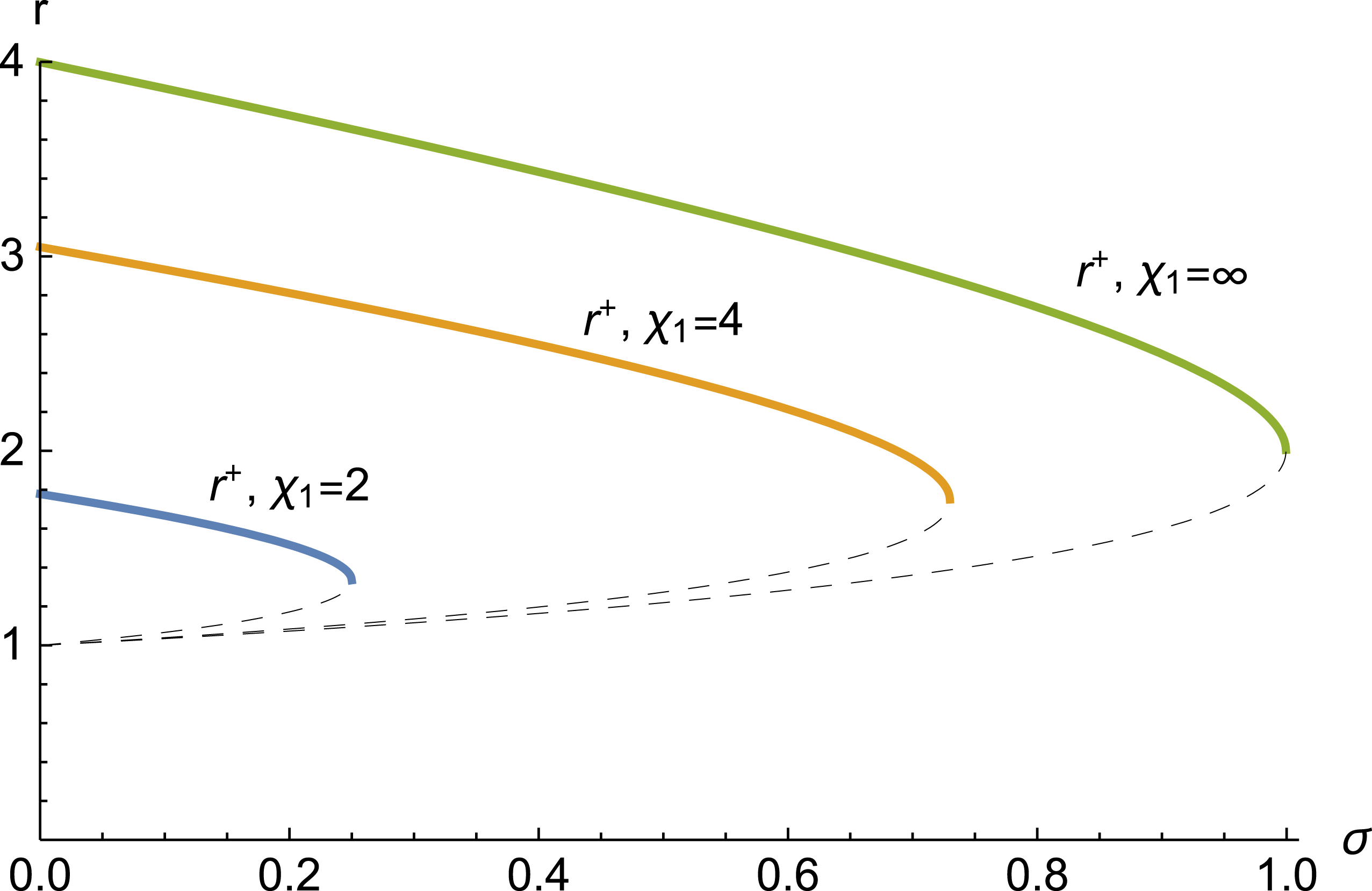
The density ratio defined by (3.5) is plotted in figure 3. For
 $\unicode[STIX]{x1D70E}=0$
and
 $\unicode[STIX]{x1D712}_{1}=\infty$
, we have
 $r^{+}=4$
and
 $r^{-}=1$
. These are the 2 solutions for the field-free problem in the strong shock limit for a 3-D gas, so that we recognize that
 $r^{+}$
corresponds to the shock solution, while
 $r_{-}$
is the trivial solution. We will focus on the
 $r_{+}$
solution.
Density jump from (3.5) as a function of
 $\unicode[STIX]{x1D70E}$
for various
 $\unicode[STIX]{x1D712}_{1}$
. The
 $r^{+}$
branch is the shock solution, shown by solid lines. The dashed lines correspond to the
 $r^{-}$
branch. The model has no solution for
 $\unicode[STIX]{x1D70E}>\unicode[STIX]{x1D70E}_{2c}$
as given by (3.6).

As an aside, note that for
 $\unicode[STIX]{x1D70E}\neq 0$
,
 $r^{-}=1$
is no longer a solution. Why is this the case? In fluid mechanics, the solution
 $r=1$
also implies the absence of velocity jump and isotropic pressure jump. Such a solution is still retrieved in our analysis of Stage 1 because imposing
 $T_{\bot }$
continuity is compatible with
 $r=1$
. Yet, by imposing the firehose threshold (1.2) in Stage 2, we forbid the
 $r=1$
solution by rendering pressure continuity impossible, unless
 $\unicode[STIX]{x1D70E}=0$
.
3.2 Anisotropy
We now come back to (2.1), which gives
 $$\begin{eqnarray}U_{2}=\frac{P_{2x}}{2n_{2}}\left(1+2\frac{P_{\bot 2}}{P_{2x}}\right)=\frac{P_{2x}}{2n_{2}}(1+2A_{2}).\end{eqnarray}$$
Inserting this result into (1.5) gives the following equation for
 $A_{2}$
,
 $$\begin{eqnarray}\frac{V_{1}^{2}}{2}+\frac{P_{1}}{n_{1}}+U_{1}=\frac{V_{2}^{2}}{2}+\frac{P_{2x}}{2n_{2}}(1+2A_{2})+\frac{P_{2x}}{n_{2}}.\end{eqnarray}$$
 $P_{2x}$
is then eliminated through (2.2). Solving for
 $A_{2}$
and introducing the variables (1.6) gives,
 $$\begin{eqnarray}A_{2}=\frac{1}{2}\frac{\unicode[STIX]{x1D712}_{1}^{2}(r-2)(r-1)+r(5r-3)}{\unicode[STIX]{x1D712}_{1}^{2}(r-1)+r}.\end{eqnarray}$$
4 Physical interpretation of the parameter
$\unicode[STIX]{x1D712}_{1}$

When computing the Rankine–Hugoniot jump conditions in a fluid, the shock solution formally extends down to zero Mach number
 ${\mathcal{M}}$
. The reason why the range of physically allowed Mach numbers is restricted to
 ${\mathcal{M}}>1$
is that the entropy jump is positive only over this range (Landau & Lifshitz Reference Landau and Lifshitz2013).
In order to make physical sense of the parameter
 $\unicode[STIX]{x1D712}_{1}$
, we therefore compute the entropy jump for both Stage 1 and Stage 2.
For a multi-temperature Maxwellian of the form,
 $$\begin{eqnarray}F=\frac{n}{\unicode[STIX]{x03C0}^{3/2}\sqrt{a}b}\exp \left(-\frac{v_{x}^{2}}{a}\right)\exp \left(-\frac{v_{y}^{2}+v_{z}^{2}}{b}\right),\end{eqnarray}$$
where
 $a=2k_{B}T_{\Vert }/m$
and
 $b=2k_{B}T_{\bot }/m$
, the entropy is
 $$\begin{eqnarray}S=-k_{B}\int F\ln F=\frac{k_{B}}{2}n[3+\ln (\unicode[STIX]{x03C0}^{3}ab^{2})-2\ln n].\end{eqnarray}$$
Computing the entropy per particle
 $s=S/n$
for the downstream and upstream plasma, we obtain the entropy jump across the shock,
 $$\begin{eqnarray}\displaystyle \frac{2}{k_{B}}\unicode[STIX]{x0394}s & = & \displaystyle \frac{2}{k_{B}}(s_{2}-s_{1})\nonumber\\ \displaystyle & = & \displaystyle \ln \left(\frac{1}{A_{2}}\frac{T_{\bot 2}^{3}}{T_{\bot 1}^{3}}\right)-2\ln r.\end{eqnarray}$$
In Stage 1, where there is no
 $T_{\bot }$
jump, we therefore have,
 $$\begin{eqnarray}\frac{2}{k_{B}}\unicode[STIX]{x0394}s=-\ln (A_{2}r^{2}).\end{eqnarray}$$
Using (2.8) we find,
 $$\begin{eqnarray}\frac{2}{k_{B}}\unicode[STIX]{x0394}s=\ln \left(\frac{(\unicode[STIX]{x1D712}_{1}^{2}-1)(3+\unicode[STIX]{x1D712}_{1}^{2})^{3}}{16\unicode[STIX]{x1D712}_{1}^{6}}\right).\end{eqnarray}$$
It is easily checked that
 $\unicode[STIX]{x2202}\unicode[STIX]{x0394}s/\unicode[STIX]{x2202}\unicode[STIX]{x1D712}_{1}>0,\forall \unicode[STIX]{x1D712}_{1}>0$
, and that
 $\unicode[STIX]{x0394}s=0$
for
 $\unicode[STIX]{x1D712}_{1}=\sqrt{3}$
. Hence, only
 $\unicode[STIX]{x1D712}_{1}>\sqrt{3}$
is physically meaningful. We could therefore have defined a Mach number in Stage 1 through
 ${\mathcal{M}}_{1}^{2}=n_{1}V_{1}^{2}/3P_{1}$
, consistent with an adiabatic index
 $\unicode[STIX]{x1D6E4}_{1D}=3$
for a 1-D system. Indeed, since we freeze the perpendicular temperature, the system becomes effectively one-dimensional. This can also be seen from (2.8), which tends to
 $r=2=(\unicode[STIX]{x1D6E4}_{1D}+1)/(\unicode[STIX]{x1D6E4}_{1D}-1)$
in the strong shock limit, and is larger than unity only for
 $\unicode[STIX]{x1D712}_{1}>\sqrt{3}$
.
For Stage 2, we start again from (4.3). Setting
 $T_{\bot 1}=T_{1}=P_{1}/n_{1}k_{B}$
and
 $T_{\bot 2}=A_{2}T_{\Vert 2}=A_{2}P_{2x}/n_{2}k_{B}$
, we obtain,
 $$\begin{eqnarray}\frac{2}{k_{B}}\unicode[STIX]{x0394}s=\ln \left(\frac{r^{5}}{A_{2}^{2}}\frac{P_{1}^{3}}{P_{2x}^{3}}\right).\end{eqnarray}$$
The anisotropy
 $A_{2}$
is now given in terms of
 $r$
and
 $\unicode[STIX]{x1D712}_{1}$
by (3.9). In turn, the density jump
 $r$
can be expressed in terms of
 $\unicode[STIX]{x1D712}_{1}$
and
 $\unicode[STIX]{x1D70E}$
through the
 $r_{+}$
branch of (3.5). Finally, equation (3.3) allows us to express
 $P_{2x}$
in terms of
 $\unicode[STIX]{x1D712}_{1}$
and
 $\unicode[STIX]{x1D70E}$
.
Through some manipulations, one can prove
 $\unicode[STIX]{x0394}s=0$
for
 $\unicode[STIX]{x1D712}_{1}=\sqrt{5/3}$
and
 $\unicode[STIX]{x1D70E}=0$
. Stage 2 is therefore physically meaningful only for
 $\unicode[STIX]{x1D712}_{1}>\sqrt{5/3}$
, which is consistent with the definition of a 3-D Mach number for this model, with
 ${\mathcal{M}}_{1}^{2}=n_{1}V_{1}^{2}/(5/3)P_{1}$
. As a consequence, the density jump is not physical in Stage 2 for
 $\unicode[STIX]{x1D712}_{1}<\sqrt{5/3}$
, and one can check from (3.6) that
 $\unicode[STIX]{x1D70E}_{2c}(\unicode[STIX]{x1D712}_{1}=\sqrt{5/3})=0$
.
At this juncture, one might think that, for
 $\unicode[STIX]{x1D712}_{1}\in [\sqrt{5/3},\sqrt{3}]$
, our model predicts the downstream will simply settle down in Stage 2. However, this is not the case. The ansatz we made for the plasma imposes Stage 1 as the first stage of its downstream history. If
 $\unicode[STIX]{x1D712}_{1}<\sqrt{3}$
, there can be no Stage 1 shock, since such a shock would cause the entropy to decrease. Since there is no Stage 1 shock, there is no option for the gas to proceed further to Stage 2. Thus, the flow will be shock free. In other words, our shock scenario makes physical sense only for
 $\unicode[STIX]{x1D712}_{1}>\sqrt{3}$
.
Could the plasma ‘shortcut’ Stage 1, and jump directly to Stage 2 when
 $\unicode[STIX]{x1D712}_{1}\in [\sqrt{5/3},\sqrt{3}]$
? This is hard to say. In the picture we have developed in this paper, the ‘Stage 1
 $\rightarrow$
Stage 2’ switch happens only if Stage 1 is unstable. The plasma therefore comes to Stage 2, from an unstable position. As the downstream plasma migrates towards stability, it will therefore cross the firehose threshold coming from an unstable position, and it settles down at the stability boundary. In contrast, if Stage 1 cannot be attained because a 1-D shock is unphysical (
 $\unicode[STIX]{x1D712}_{1}<\sqrt{3}$
,
 $\unicode[STIX]{x0394}s<0$
), then the stable downstream plasma has no reason to lie on the firehose stability threshold. In that case, the anisotropy cannot be related to the field in a deterministic way, for the range of stable possibilities is infinite, as illustrated on figure 1.
Therefore, if we wish to define the ‘usual’ Mach number, that is,
 ${\mathcal{M}}_{1}^{2}=n_{1}V_{1}^{2}/(5/3)P_{1}=(3/5)\unicode[STIX]{x1D712}_{1}^{2}$
, our model offers physical solutions only for
 ${\mathcal{M}}_{1}>3/\sqrt{5}\sim 1.34$
.
Is this Mach number restriction physical, or simply an artefact of our model? As stated in the introduction, the fluid is disconnected from the field for a strictly parallel MHD shock. As a consequence, the minimum Mach number in the MHD regime is simply 1. Although to our knowledge no systematic study of weak collisionless shocks has been conducted so far, the
 ${\mathcal{M}}_{1}>3/\sqrt{5}$
restriction is probably an artefact of our model.
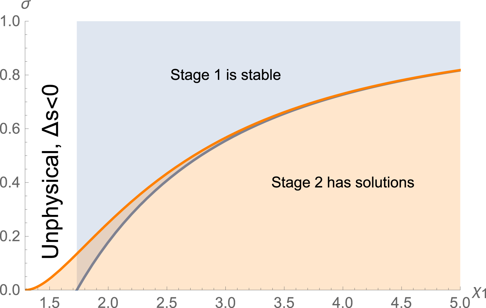
The downstream in Stage 1 is stable in the shaded blue area, and gives an entropy increase at the front only for
 $\unicode[STIX]{x1D712}_{1}>\sqrt{3}\sim 1.7$
. Stage 2 has solutions in the shaded orange region and gives an entropy increase at the front only for
 $\unicode[STIX]{x1D712}_{1}>\sqrt{5/3}\sim 1.3$
. Since our ansatz assumes the plasma goes first through Stage 1, our model is not physical for
 $\unicode[STIX]{x1D712}_{1}<\sqrt{3}$
(see discussion in § 4).

5 Transition from Stage 1 to Stage 2
We have seen that Stage 2 has solutions only for
 $\unicode[STIX]{x1D70E}<\unicode[STIX]{x1D70E}_{2c}$
(3.6), while Stage 1 is stable only for
 $\unicode[STIX]{x1D70E}>\unicode[STIX]{x1D70E}_{1c}$
(2.11). Figure 4 shows the domains defined by these inequalities in the
 $(\unicode[STIX]{x1D712}_{1},\unicode[STIX]{x1D70E})$
plane.
Notably, the difference
 $(\unicode[STIX]{x1D70E}_{1c}-\unicode[STIX]{x1D70E}_{2c})$
goes to zero like
 $\unicode[STIX]{x1D712}_{1}^{-4}$
in the strong shock limit, so that both regions are exactly complimentary in this regime. We present a few results in this limit before we deal with intermediate values of
 $\unicode[STIX]{x1D712}_{1}$
.
5.1 Results for strong shocks,
$\unicode[STIX]{x1D712}_{1}\gg 1$

Consider the case
 $\unicode[STIX]{x1D712}_{1}\rightarrow \infty$
. For small values of
 $\unicode[STIX]{x1D70E}$
, the point representing the system in figure 4 lies in the orange region. For larger
 $\unicode[STIX]{x1D70E}$
, the system lies in the blue region. As can be seen on the figure, the blue and the orange regions do not overlap in the strong shock limit. Therefore, in this limit, the system is either stable on Stage 1 (high
 $\unicode[STIX]{x1D70E}$
), or firehose stable on Stage 2 because stage 1 was unstable (low
 $\unicode[STIX]{x1D70E}$
).
Some useful analytical results can be derived in this regime.
Stage 1 is stable beyond
 $\unicode[STIX]{x1D70E}=\unicode[STIX]{x1D70E}_{1c}=1$
. The density jump is
 $r_{\infty }=2$
, and the anisotropy
 $A_{2\infty }\sim 4/\unicode[STIX]{x1D712}_{1}^{2}\rightarrow 0$
as
 $\unicode[STIX]{x1D712}_{1}\rightarrow \infty$
.
For
 $\unicode[STIX]{x1D70E}<\unicode[STIX]{x1D70E}_{2c}=1$
, Stage 2 has stable solutions. The density jump in Stage 2 reads,
 $$\begin{eqnarray}r_{\infty }(\unicode[STIX]{x1D70E})=\frac{1}{2}\left(\sqrt{(\unicode[STIX]{x1D70E}-9)(\unicode[STIX]{x1D70E}-1)}+5-\unicode[STIX]{x1D70E}\right),\end{eqnarray}$$
with
 $r_{\infty }(0)=4$
and
 $r_{\infty }(1)=2$
(see figure 5). The anisotropy is given by
 $$\begin{eqnarray}A_{2\infty }(\unicode[STIX]{x1D70E})=\frac{1}{4}\left(\sqrt{(\unicode[STIX]{x1D70E}-9)(\unicode[STIX]{x1D70E}-1)}+1-\unicode[STIX]{x1D70E}\right),\end{eqnarray}$$
with
 $A_{2\infty }(0)=1$
and
 $A_{2\infty }(\unicode[STIX]{x1D70E}\sim 1)\sim \sqrt{(1-\unicode[STIX]{x1D70E})/2}\rightarrow 0$
as
 $\unicode[STIX]{x1D70E}\rightarrow 1$
.
Equations (5.1), (5.2) clearly show that the anisotropy follows the same profile as the density ratio. Therefore, when
 $\unicode[STIX]{x1D70E}=0$
, the strong shock is isotropic, with
 $A_{2}=1$
. For small
 $\unicode[STIX]{x1D70E}$
, the downstream anisotropy
 $A_{2}$
is given (5.2), which pertains to stage 2. For
 $\unicode[STIX]{x1D70E}=1$
and beyond, the system can remain in Stage 1, which is stabilized by the field. The anisotropy parameter is
 $A_{2}=0$
(see (2.8) in the limit
 $\unicode[STIX]{x1D712}_{1}\rightarrow \infty$
) all the way up to
 $\unicode[STIX]{x1D70E}=\infty$
.
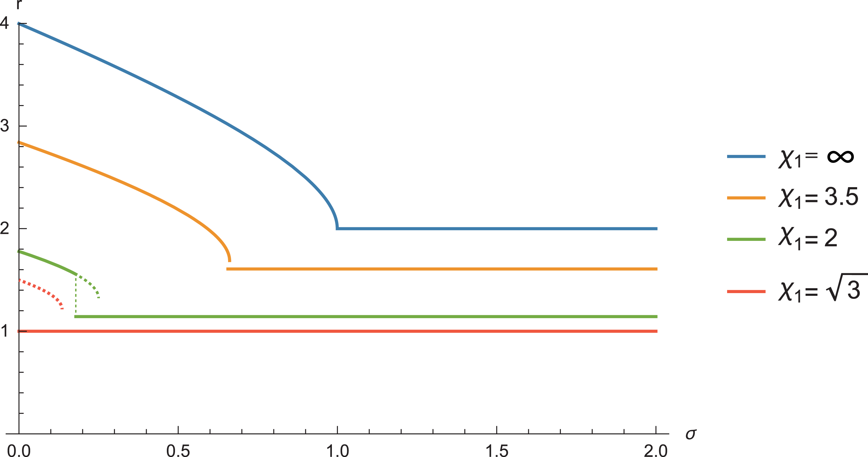
Density jump as a function of
 $\unicode[STIX]{x1D70E}$
for various values of
 $\unicode[STIX]{x1D712}_{1}$
. Whenever Stage 1 (horizontal lines) and Stage 2 (curved lines) both have stable solutions, the physical one is Stage 1 (see § 5.2). Stage 2 density jump is plotted for
 $\unicode[STIX]{x1D70E}\in [0,\unicode[STIX]{x1D70E}_{2c}]$
. Stage 1 density jump is plotted for
 $\unicode[STIX]{x1D70E}\in [\unicode[STIX]{x1D70E}_{1c},2]$
.

5.2 Intermediate values of
$\unicode[STIX]{x1D712}_{1}$

For intermediate values of
 $\unicode[STIX]{x1D712}_{1}$
, for example
 $\unicode[STIX]{x1D712}_{1}=2$
, and small
 $\unicode[STIX]{x1D70E}$
, figure 4 shows that Stage 1 is unstable. The system therefore goes to Stage 2, which offers solutions. Yet, for slightly larger values of
 $\unicode[STIX]{x1D70E}$
, while Stage 1 is stable, at the same time Stage 2 also offers a solution. Which stage should the system ‘choose’? According to the plasma history we propose, the system goes first through Stage 1, before it switches to Stage 2, and the switch happens only if Stage 1 is unstable. As a consequence, when stable, Stage 1 is always the physical solution. If not, the downstream plasma moves to Stage 2 which becomes its final state.
The density jump
 $r$
is eventually plotted in terms of
 $\unicode[STIX]{x1D70E}$
in figure 5. The solution is given by Stage 2 at low
 $\unicode[STIX]{x1D70E}$
, and by Stage 1 at high
 $\unicode[STIX]{x1D70E}$
. When the function
 $r(\unicode[STIX]{x1D70E})$
is multi-valued because Stage 1 is stable while Stage 2 offers a solution, the physical solution is given by Stage 1. In such cases, we plotted the Stage 2 solution in dashed line. As evidenced, the departure from the MHD prediction (no-
 $\unicode[STIX]{x1D70E}$
dependence) increases with
 $\unicode[STIX]{x1D70E}$
.
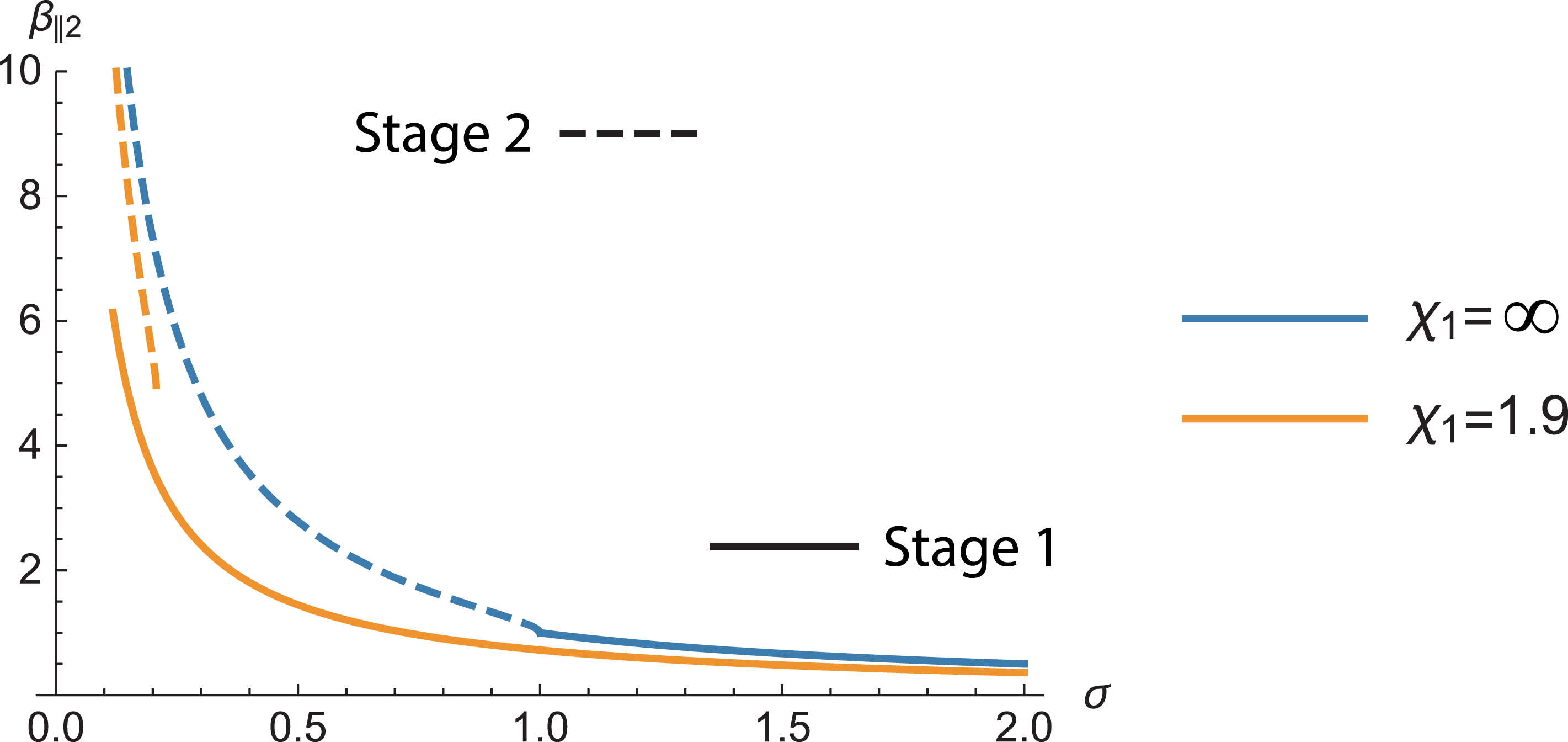
Value of
 $\unicode[STIX]{x1D6FD}_{\Vert 2}$
as a function of
 $\unicode[STIX]{x1D70E}$
for Stage 1 (plain lines) and Stage 2 (dashed lines), and
 $\unicode[STIX]{x1D712}_{1}=1.9$
and
 $\infty$
. If
 $\unicode[STIX]{x1D70E}$
is such that it stabilizes Stage 1 while Stage 2 offers a solution, then the
 $\unicode[STIX]{x1D6FD}_{\Vert 2}$
of the downstream is given by Stage 1.

6 Locating the system in figure 1
Although the description of the problem in terms of the parameters
 $(\unicode[STIX]{x1D70E},\unicode[STIX]{x1D712}_{1})$
is particularly adapted to PIC simulations, it is instructive to locate the system in figure 1, in terms of the parameters
 $(\unicode[STIX]{x1D6FD}_{\Vert 2},T_{\bot 2}/T_{\Vert 2})$
.
The anisotropy
 $A_{2}=T_{\bot 2}/T_{\Vert 2}$
is given by (2.8) for Stage 1 and by (3.9) for Stage 2. Regarding the parameter
 $\unicode[STIX]{x1D6FD}_{\Vert 2}$
, it is given by (2.9) for Stage 1. For Stage 2, it is readily derived from (1.2) in terms of the anisotropy (3.9), since the firehose stability threshold is assumed for this stage.
Let us start by plotting
 $\unicode[STIX]{x1D6FD}_{\Vert 2}$
as a function of
 $\unicode[STIX]{x1D70E}$
for both stages (figure 6). At large
 $\unicode[STIX]{x1D70E}$
, Stage 1 is stable, so that the
 $\unicode[STIX]{x1D6FD}_{\Vert 2}$
of the downstream is given by this part of the plots (solid lines). For smaller values of
 $\unicode[STIX]{x1D70E}$
, when Stage 1 becomes unstable, the
 $\unicode[STIX]{x1D6FD}_{\Vert 2}$
of the downstream is given by the Stage 2 part of the plots (dashed lines). If
 $\unicode[STIX]{x1D70E}$
is such that it stabilizes Stage 1 while Stage 2 also offers a solution,
 $\unicode[STIX]{x1D6FD}_{\Vert 2}$
is given by Stage 1.
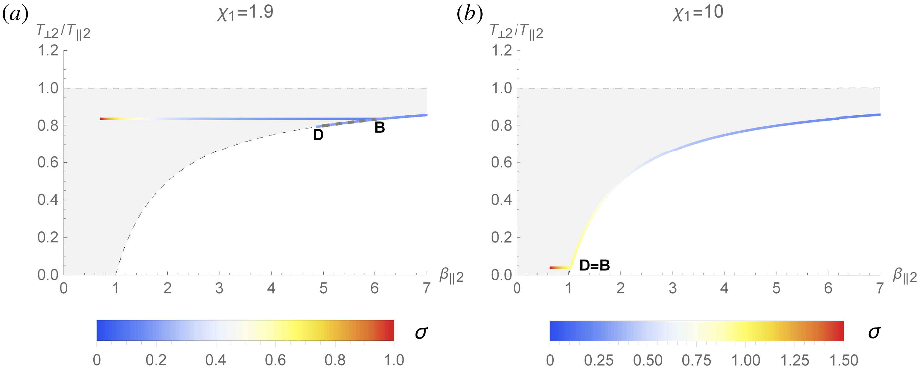
Location of the system in figure 1, in terms of
 $\unicode[STIX]{x1D70E}$
. For
 $\unicode[STIX]{x1D712}_{1}=1.9$
, there is a range of
 $\unicode[STIX]{x1D70E}$
where Stage 1 is stable while Stage 2 offers solutions. In this case, the system settles in Stage 1, namely, the first stage of its post-front history. For this reason, the portion D–B of the firehose curve is dashed since the system will not sweep it.

We can now turn to figure 7 which locates the system on figure 1. For both values of
 $\unicode[STIX]{x1D712}_{1}$
shown we plot the parametric curve,
 $$\begin{eqnarray}\displaystyle & \displaystyle X=\unicode[STIX]{x1D6FD}_{\Vert 2}(\unicode[STIX]{x1D70E}), & \displaystyle\end{eqnarray}$$
 $$\begin{eqnarray}\displaystyle & \displaystyle Y=A_{2}(\unicode[STIX]{x1D70E}). & \displaystyle\end{eqnarray}$$
The resulting curves are coloured in terms of
 $\unicode[STIX]{x1D70E}$
. The point representing the downstream moves from right to left with increasing
 $\unicode[STIX]{x1D70E}$
. For
 $\unicode[STIX]{x1D70E}\equiv \unicode[STIX]{x1D70E}_{B}$
, the downstream is represented by point B of figures 1 and 7. For
 $\unicode[STIX]{x1D70E}=\unicode[STIX]{x1D70E}_{B}+\unicode[STIX]{x1D700}$
, Stage 1 becomes stable while Stage 2 still has solutions. For Stage 2, the corresponding part of the curve is the short dashed B–D line in figure 1, along the firehose threshold. This double solution is particularly visible on figure 7(a), for
 $\unicode[STIX]{x1D712}_{1}=1.9$
. For
 $\unicode[STIX]{x1D712}_{1}=10$
, B and D are almost superimposed.
As explained previously, as soon as Stage 1 is stable, it is also the physical solution since our plasma first goes through this stage in the course of its downstream history. As a consequence, the system will not experience the B–D states of Stage 2 in figure 1. In case
 $\unicode[STIX]{x1D70E}$
is in the corresponding range, the plasma will simply settle in the solution offered by Stage 1, namely, settle in the first stage of its post-front history.
7 Conclusions
In order to derive an expression for the downstream temperature anisotropy in terms of the field strength in a parallel collisionless shock, we postulated a particular history for the plasma. As it crosses the shock front, the plasma goes through the first stage of its history, namely ‘Stage 1’, characterized by
 $T_{\bot 2}=T_{\bot 1}$
. Stage 1 has
 $T_{\bot 2}/T_{\Vert 2}<1$
and may or may not be firehose unstable. If the magnetic field is strong enough for Stage 1 to be stable, then the plasma remains in this state. However, if Stage 1 is firehose unstable, the plasma moves to a new state located on the firehose stability threshold line. This is ‘Stage 2’.
In both Stage 1 and Stage 2, the conservation equations permit a complete solution for the downstream properties of the plasma, including the temperature anisotropy parameter
 $A_{2}$
. From this analysis, an effective adiabatic index
 $\unicode[STIX]{x1D6E4}$
can be computed from first principles. We start by writing the downstream internal energy as
 $U_{2}=((1+2A_{2})/2n_{2})P_{x2}\equiv P_{x2}/(\unicode[STIX]{x1D6E4}-1)$
, so that,
 $$\begin{eqnarray}\unicode[STIX]{x1D6E4}=\frac{3+2A_{2}}{1+2A_{2}}\end{eqnarray}$$
fulfilling therefore
 $\unicode[STIX]{x1D6E4}(\unicode[STIX]{x1D70E}=0)=5/3$
and
 $\unicode[STIX]{x1D6E4}(\unicode[STIX]{x1D70E}>1)=3$
.
The large-
 $\unicode[STIX]{x1D70E}$
plateau in the density jump observed in figure 5 is likely an artefact of our
 $T_{\bot }=$
constant hypothesis, rather than a real physical feature. For the strong shock case, for example, we do expect
 $\lim _{\unicode[STIX]{x1D70E}\rightarrow \infty }r=2$
, which the double adiabatic theory reproduces successfully. Yet, this theory turns exact only in the infinite
 $\unicode[STIX]{x1D70E}$
limit, where the Larmor radius is smaller than all the other length scales, shock front thickness included. But for moderate
 $\unicode[STIX]{x1D70E}$
, the dissipation/heating occurring at the front should cause the plasma to deviate from
 $T_{\bot }=$
constant, even though the field may be strong enough to stabilize the first stage of the post-front evolution. The function
 $r(\unicode[STIX]{x1D70E})$
is thus likely to be smoother than in our model.
This is indeed what was observed in Bret et al. (Reference Bret, Pe’er, Sironi, SaḐowski and Narayan2017). These simulations were relativistic, so that the non-relativistic theory described here cannot be directly compared to the numerical results. Forthcoming works should therefore focus on numerically testing the present theory.
As emphasized in the introduction, parallel shocks are excellent test beds to study departures from MHD, since according to MHD, the field and the fluid are disconnected. In such a configuration, any variation of shock properties with the field strength must be a kinetic effect. Yet, an effective adiabatic index like (7.1) has to be obliquity dependent if it is to be incorporated in MHD codes. Extending the present theory to oblique and perpendicular shocks is therefore necessary.
It should be possible to adapt the present treatment to perpendicular shocks by considering the consequences of the double adiabatic theory for such systems. Instead of having
 $T_{\bot }$
conserved and
 $T_{\Vert }$
increased through the front, we would have
 $T_{\bot }\propto B$
increased by the density ratio,Footnote
3
and
 $T_{\Vert }\propto (n/B)^{2}$
, constant. Stage 1 in the downstream will therefore have
 $T_{\bot }/T_{\Vert }>1$
, for which stability will be governed by the mirror instability (Vogl et al.
Reference Vogl, Biernat, Erkaev, Farrugia and Mühlbachler2001).
It would be useful to extend this work to the relativistic regime and the case of electron/ion plasmas, or even to account for the role of reflected particles at the front. Relativistic effects will affect the conservation equations, the stability thresholds and the double adiabatic invariants (Scargle Reference Scargle1968). As already alluded to in the introduction, considering electron/ion plasmas may introduce temperature differences between species and extra physics downstream, whose roles are unclear at this stage. Finally, reflected particles may impact the conservation equations and the double adiabatic invariants.
Acknowledgements
A.B. acknowledges support by grants ENE2016-75703-R from the Spanish Ministerio de Educación and SBPLY/17/180501/000264 from the Junta de Comunidades de Castilla-La Mancha. R.N. acknowledges support from the NSF via grant AST-1816420. A.B. thanks the Black Hole Initiative (BHI) at Harvard University for hospitality, and R.N. thanks the BHI for support. The BHI is funded by a grant from the John Templeton Foundation. The authors thank R. Schlickeiser and M. Gedalin for valuable inputs, and the two referees for numerous helpful comments.