1. Introduction
Turbulence in the presence of a mean velocity gradient is a fundamental problem relevant to many flows in physics and engineering. Internal flows with varying cross-section experience mean strain arising from streamwise variation of the mean velocity (Ayyalasomayajula & Warhaft Reference Ayyalasomayajula and Warhaft2006). Mean strain also plays an important role in the flow near stagnation points around bluff bodies (Li et al. Reference Li, Li, Yang, Li, Wang and Huang2024). Another important example is turbulence under mean shear, as observed in jets, wakes and boundary layers. The mean velocity gradient tensor
 $\unicode{x1D63C}$
is defined as
 \begin{align} {\unicode{x1D63C}}= \begin{pmatrix} \partial \langle u\rangle /\partial x & \partial \langle u\rangle /\partial y & \partial \langle u\rangle /\partial z \\ \partial \langle v\rangle /\partial x & \partial \langle v\rangle /\partial y & \partial \langle v\rangle /\partial z \\ \partial \langle w\rangle /\partial x & \partial \langle w\rangle /\partial y & \partial \langle w\rangle /\partial z \end{pmatrix}\!, \end{align}
where
 $u$
,
 $v$
and
 $w$
are the velocity components in the
 $x$
,
 $y$
and
 $z$
directions, respectively, and
 $\langle \boldsymbol{\cdot }\rangle$
denotes an average. Hereafter, vector and tensor components are denoted by subscripts corresponding to the
 $x$
,
 $y$
and
 $z$
directions; for example,
 $\mathsf{A}_{\textit{xx}} = \partial u/\partial x$
. Fundamental studies of turbulence often consider specific forms of
 $\mathsf{A}_{\textit{ij}}$
. For example, simple mean shear corresponds to
 $\mathsf{A}_{\textit{ij}}$
having a single non-zero off-diagonal component, with all other components equal to zero. Other cases involve irrotational mean strains, characterised by the diagonal components of
 $\mathsf{A}_{\textit{ij}}$
. A typical example is axisymmetric strain, which can be classified into two forms: axisymmetric contraction and axisymmetric expansion, represented by
 \begin{align} {\unicode{x1D63C}}= \begin{pmatrix} S & 0 & 0 \\ 0 & -S/2 & 0 \\ 0 & 0 & -S/2 \end{pmatrix} \quad \textrm {for axisymmetric contraction} \end{align}
and
 \begin{align} {\unicode{x1D63C}}= \begin{pmatrix} -S & 0 & 0 \\ 0 & S/2 & 0 \\ 0 & 0 & S/2 \end{pmatrix} \quad \textrm {for axisymmetric expansion}, \end{align}
with strain rate
 $S \gt 0$
. The distinction between these two forms is illustrated by the deformation of a fluid element. Under axisymmetric contraction, a spherical element is elongated along the symmetry axis and compressed in the transverse directions, forming a rugby-ball-like shape. In contrast, under axisymmetric expansion, the element is compressed along the axis and stretched transversely, forming a flattened, pancake-like shape. Mean deformation due to shear and strain, described by
 $\unicode{x1D63C}$
, influences turbulence through production, dissipation and redistribution of turbulent kinetic energy across scales and space and the development of anisotropy (Keffer Reference Keffer1965; Pope Reference Pope2000). The effects of mean deformation on initially homogeneous and isotropic turbulence (HIT) have long been central topics in fluid mechanics.
Axisymmetric irrotational strain is of particular interest because it represents one of the simplest anisotropic forms of
 $\mathsf{A}_{\textit{ij}}$
(Sagaut & Cambon Reference Sagaut and Cambon2018). Statistical axisymmetry enables the development of theories for strained homogeneous turbulence. A notable example is rapid distortion theory (RDT), which assumes that mean strain acts on turbulence over a time scale much shorter than that of the turbulent motions. The RDT has been employed to predict the evolution of initially HIT subjected to a sudden imposition of axisymmetric contraction or expansion (Batchelor & Proudman Reference Batchelor and Proudman1954; Lee Reference Lee1989). Related theoretical works address statistically axisymmetric turbulence without mean strain, which are applicable when turbulence is exposed to axisymmetric strain for a finite duration and subsequently evolves freely in its absence. These theoretical frameworks build upon the kinematics of axisymmetric turbulence (Batchelor Reference Batchelor1946; Chandrasekhar Reference Chandrasekhar1950; Lindborg Reference Lindborg1995). Other theories consider the decay of homogeneous axisymmetric turbulence (Davidson, Okamoto & Kaneda Reference Davidson, Okamoto and Kaneda2012) and predict decay laws under the influence of external forces such as buoyancy in stably stratified fluids or the Coriolis force due to rotation (Davidson Reference Davidson2010, Reference Davidson2013; Watanabe, Zheng & Nagata Reference Watanabe, Zheng and Nagata2022).
Turbulence subject to axisymmetric strain has also been studied using direct numerical simulation (DNS) and experiments. In DNS, uniform mean strain is introduced by deforming the computational domain (Rogallo Reference Rogallo1981). This method has been used to investigate the evolution of turbulence under a finite duration of axisymmetric contraction or expansion, followed by relaxation without strain (Zusi & Perot Reference Zusi and Perot2014; Clay & Yeung Reference Clay and Yeung2016). Similar simulations have also been conducted for planar strain (Chen, Meneveau & Katz Reference Chen, Meneveau and Katz2006; Zusi & Perot Reference Zusi and Perot2013). Also, DNS has been used to explore the behaviour of particles seeded in turbulence subject to axisymmetric expansion (Gylfason et al. Reference Gylfason, Lee, Perlekar and Toschi2011). Relevant wind tunnel experiments have been carried out for grid-generated turbulence passing through a contracting section, where the streamwise variation of tunnel cross-section induces axisymmetric contraction (Uberoi Reference Uberoi1956). Turbulence is strongly modified while traversing the contracting section, followed by relaxation in the downstream region of constant cross-section. Many experimental investigations have thus focused on axisymmetric contraction (Hussain & Ramjee Reference Hussain and Ramjee1976; Sjögren & Johansson Reference Sjögren and Johansson1998; Ayyalasomayajula & Warhaft Reference Ayyalasomayajula and Warhaft2006; Ertunç & Durst Reference Ertunç and Durst2008; Alhareth et al. Reference Alhareth, Mugundhan, Langley and Thoroddsen2024). Other related examples include experiments on turbulence subject to planar contraction, in which the mean strain consists of expansion and contraction along two orthogonal directions (Thoroddsen & Van Atta Reference Thoroddsen and Van Atta1995; Brown, Parsheh & Aidun Reference Brown, Parsheh and Aidun2006; Mugundhan et al. Reference Mugundhan, Pugazenthi, Speirs, Samtaney and Thoroddsen2020). Experimental studies on axisymmetric expansion are far fewer than those on contraction. One example of axisymmetric expansion is grid turbulence passing through a diverging section (Choi & Lumley Reference Choi and Lumley2001). Another example utilises a facility comprising two opposing discs moving towards each other in a water tank (Liu, Katz & Meneveau Reference Liu, Katz and Meneveau1999; Hassanian et al. Reference Hassanian, Helgadóttir, Bouhlali and Riedel2023).
Most experimental studies on turbulence subject to axisymmetric strain have focused on contraction. Investigations of turbulence subject to axisymmetric contraction have consistently shown that nonlinear effects play a major role in the influence of mean strain, leading to deviations from RDT predictions. The measured energy spectrum exhibits increasingly pronounced departures from RDT at higher Reynolds numbers (Ayyalasomayajula & Warhaft Reference Ayyalasomayajula and Warhaft2006), highlighting the importance of high-Reynolds-number investigations for clarifying the effects of mean strain. However, previous laboratory studies of axisymmetric expansion have predominantly been conducted at lower Reynolds numbers. The present study introduces a new facility that realises turbulence subject to axisymmetric expansion at high Reynolds numbers. The facility comprises two multiple-jet generators, each producing decaying, nearly HIT through jet interaction. The opposed jet arrays generate two turbulent flows that collide and form a mean-flow stagnation point, thereby establishing axisymmetric strain. The role of the two arrays is to establish axisymmetric expansion in the stagnation region from initially nearly homogeneous, isotropic inflows generated by each array. A turbulent flow issuing from a single jet nozzle exhibits a highly inhomogeneous transverse distribution of velocity statistics. By contrast, interaction among many jets within a confined test section forms nearly HIT, with velocity statistics homogeneous across the cross-sectional planes (Tan et al. Reference Tan, Xu, Qi and Ni2023; Mori, Watanabe & Nagata Reference Mori, Watanabe and Nagata2024). This configuration is consistent with theories and numerical simulations that explore mean-strain effects on initially isotropic turbulence and is well suited to examine departures from isotropy caused by mean strain. The multiple-jet generator is identical to that used in our previous studies (Mori et al. Reference Mori, Watanabe and Nagata2024; Watanabe et al. Reference Watanabe, Mori, Ishizawa and Nagata2024, Reference Watanabe, Inagaki, Mori, Ishizawa and Nagata2025), where the formation and decay of nearly HIT were characterised using particle image velocimetry (PIV). In those works, the turbulent Reynolds number based on the Taylor microscale reached values as high as 750, exceeding those attained in earlier experiments on turbulence subject to axisymmetric expansion.
In the present study, we perform PIV measurements to characterise turbulence under axisymmetric expansion. Because high-speed jet interaction generates high-Reynolds-number turbulence, the present data are well suited to assess the effects of axisymmetric expansion on inertial-range scalings of velocity fluctuations, which have not been examined in previous studies. Previous studies on turbulence subject to axisymmetric expansion primarily addressed anisotropy via one-point statistics; Reynolds-number limitations hindered discussion of spectral and structure–function behaviour. The present results demonstrate anisotropy introduced by the expansion and reveal deviations in energy spectra and structure functions from predictions based on RDT or Kolmogorov’s second similarity hypothesis.
The paper is organised as follows. Section 2 describes the turbulence facility and the measurement techniques. Section 3 presents the experimental results, including the mean flow field and statistical properties of velocity fluctuations. Finally, the main findings are summarised in § 4.
2. Experimental set-up and measurement methods
2.1. Opposed multiple-jet array facility
The Opposed Multiple-Jet Array (OMJA) facility consists of two multiple-jet generators and a test section. A photograph of the OMJA is shown in figure 1, and a schematic is illustrated in figure 2. The jet direction is denoted by
 $x$
, the vertical direction by
 $y$
and the remaining direction by
 $z$
. A total of
 $6 \times 6$
jets are issued from each generator into the inner ducts. These jets interact and evolve into nearly HIT as they pass through the ducts, as reported in our previous study (Mori et al. Reference Mori, Watanabe and Nagata2024). Here, in wind tunnel experiments of decaying HIT, ‘homogeneous’ typically refers to the cross-sectional plane, while streamwise inhomogeneity persists due to decay (Comte-Bellot & Corrsin Reference Comte-Bellot and Corrsin1966). The opposed turbulent flows collide near the centre of the test section after exiting the inner ducts, spread radially towards the outer duct and then discharge from the section. The inner and outer ducts have square cross-sections of
 $100 \times 100$
mm
 $^2$
and
 $200 \times 200$
mm
 $^2$
, respectively. The collision of the opposed flows generates a mean strain field around the test-section centre. As shown below, the mean strain comprises compression in the
 $x$
direction and expansion in the
 $y$
and
 $z$
directions, approximating axisymmetric expansion. As the turbulent flows from the opposing jet arrays approach the test-section centre and then proceed towards the outer duct, they experience the mean strain for longer durations, leading to accumulated-strain effects. Consequently, in the present set-up the flow is expected to be inhomogeneous. Velocity measurements are conducted in the central region to characterise turbulence influenced by the mean strain. The facility details are described below.
Photograph of the OMJA facility.

Schematic of the OMJA facility. All dimensions are in millimetres. All components appear in pairs except the outer duct. The inner ducts have a square cross-section of
 $100^2$
mm
 $^2$
. The outer duct has a square cross-section of
 $200^2$
mm
 $^2$
and length of 300 mm. Coordinates
 $x$
,
 $y$
and
 $z$
denote the jet-flow, vertical and lateral directions, respectively. Each plenum chamber is equipped with
 $6\times 6$
Laval nozzles with inlet, throat and outlet diameters of 6.3 , 4.12 and 4.31 mm, respectively. The spacing between adjacent nozzles is
 $M=12$
mm, and the nozzle outer diameter is 7.5 mm. The inner-duct length and the nozzle-to-nozzle spacing between the two jet arrays are denoted by
 $D_I$
and
 $D_N$
, which determine the gap between the inner-duct ends as
 $D_E=D_N-2D_I$
.

Two identical jet generators and air-supply systems are placed on either side of the test section. Compressed air is stored in two 400 l tanks (Anest Iwata, SAT-400C-140) pressurised by oil-free compressors (Anest Iwata, TFP75CF-10). The compressed air is dried and cooled by refrigerant-type dryers (Orion Machinery, RAX8J-SE-A1) before entering the tanks. Downstream of the tanks, the pneumatic system comprises moisture separators (SMC, AF800-14), pressure regulators (SMC, AR825-14G) and solenoid valves (SMC, VXP2380-14-5G). When the solenoid valves are opened, compressed air at the regulated pressure is supplied to each plenum chamber. All pipes and fittings between the tanks and chambers have a nominal size of JIS 40A, corresponding to an inner diameter of approximately 40 mm.
Each jet generator consists of a plenum chamber made from a stainless steel pipe with an inner diameter of 155.2 mm and a length of 160 mm. Two chambers are mounted on a single aluminium frame, allowing adjustment of their positions in the
 $x$
direction. One end of each chamber is connected to the air supply system via a stainless steel flange, and the endplate facing the test section is fitted with a nozzle plate containing
 $6 \times 6$
Laval nozzles. The endplate also features a pressure port connected to pressure sensors. The internal geometry of the nozzle is shown in figure 2. The nozzle inlet, throat and outlet diameters are 6.3 , 4.12 and 4.31 mm, respectively. The first 5 mm from the inlet has a constant diameter of 6.3 mm. The diameter in the convergent section is reduced to 4.12 mm at the throat over 11.5 mm following a cosine function of the streamwise location. In a diverging section, the diameter increases to 4.31 mm at the outlet. The diameter profile in the diverging section is determined analytically (Foelsch Reference Foelsch1949). The nozzles are designed to produce fully expanded supersonic jets with a Mach number
 $M_{\!J} = U_{\!J}/a_{\!J} = 1.36$
and a jet Reynolds number
 $\textit{Re}_{\!J} = \rho _{\!J} U_{\!J} D / \mu _{\!J} =1.9 \times 10^5$
at a plenum pressure of 300 kPa, where
 $U_{\!J}=404$
m s−1 is the jet velocity,
 $D=4.31$
mm is the jet exit diameter,
 $a_{\!J}=297$
m s−1 is the speed of sound,
 $\rho _{\!J}=1.61$
kg m−
 $^3$
is the density and
 $\mu _{\!J}=1.44\times 10^{-5}$
Pa s is the kinematic viscosity. These fluid properties refer to the flow state at the nozzle outlet and are determined based on the nozzle design. The spacing between adjacent nozzles is
 $M=12$
mm and the outer nozzle diameter is 7.5 mm, as shown in figure 2. The nozzle plate is fixed to the plenum chamber endplate using seal washers, nuts and a 1 mm thick PTFE gasket sheet to prevent leakage. We define the reference velocity and length scales for turbulence generation as the jet velocity
 $U_{\!J}$
and the jet spacing
 $M$
, which are used to normalise the results.
All technical specifications of the jet generators, including the plenum chambers and nozzles, are identical to those in our previous studies on decaying HIT generated by jet interaction from a single jet array (Mori et al. Reference Mori, Watanabe and Nagata2024; Watanabe et al. Reference Watanabe, Mori, Ishizawa and Nagata2024, Reference Watanabe, Inagaki, Mori, Ishizawa and Nagata2025), except for a minor adjustment of chamber size in the present set-up. Although the jets are initially supersonic, mixing with the surrounding fluid significantly reduces the mean velocity. Consequently, both mean velocity and fluctuations are much lower than the speed of sound except in the near-nozzle region, and compressibility effects are locally negligible once jet interaction forms decaying nearly HIT.
The test section consists of inner and outer ducts. Two inner ducts with a square cross-section of
 $100 \times 100$
mm
 $^2$
are attached to the plenum chamber endplates. Jet interaction within each inner duct generates nearly HIT, which decays with distance from the nozzles. From the gap between the inner-duct ends, the turbulent flow enters a 300 mm long outer duct with a square cross-section of
 $200 \times 200$
mm
 $^2$
. Both ducts are constructed from clear acrylic walls supported by aluminium frames. The top wall of the outer duct contains small closable holes for inserting sensors for pressure and temperature measurements. The inner-duct length,
 $D_I$
, and the nozzle-to-nozzle spacing between the two jet arrays,
 $D_N$
, are key experimental parameters. These define the gap between the duct ends as
 $D_E = D_N - 2D_I$
. The geometric parameters are illustrated in figure 2, and their values are given below. They are varied by exchanging inner-duct components of different lengths and by adjusting the plenum chamber positions.
2.2. Experimental conditions
Prior to each experiment, the air tanks are pressurised to approximately 0.9 MPaG. Once the solenoid valves are opened, compressed air from the tanks is supplied to the plenum chambers, raising the plenum pressure. The pressure regulators are adjusted such that the plenum pressure is maintained at approximately 300 kPa, at which each nozzle is designed to generate fully expanded supersonic jets with
 $M_{\!J} = 1.36$
and
 $\textit{Re}_{\!J} = 1.9 \times 10^5$
. In our previous study, based on schlieren visualisation and the Prandtl formula (Pack Reference Pack1950), the actual jet Mach number was estimated to be about 1.33, consistent with the nozzle design (Mori et al. Reference Mori, Watanabe and Nagata2024).
Upon opening the valves,
 $6 \times 6$
jets are issued from the nozzle arrays of both generators. The plenum pressures
 $P_C$
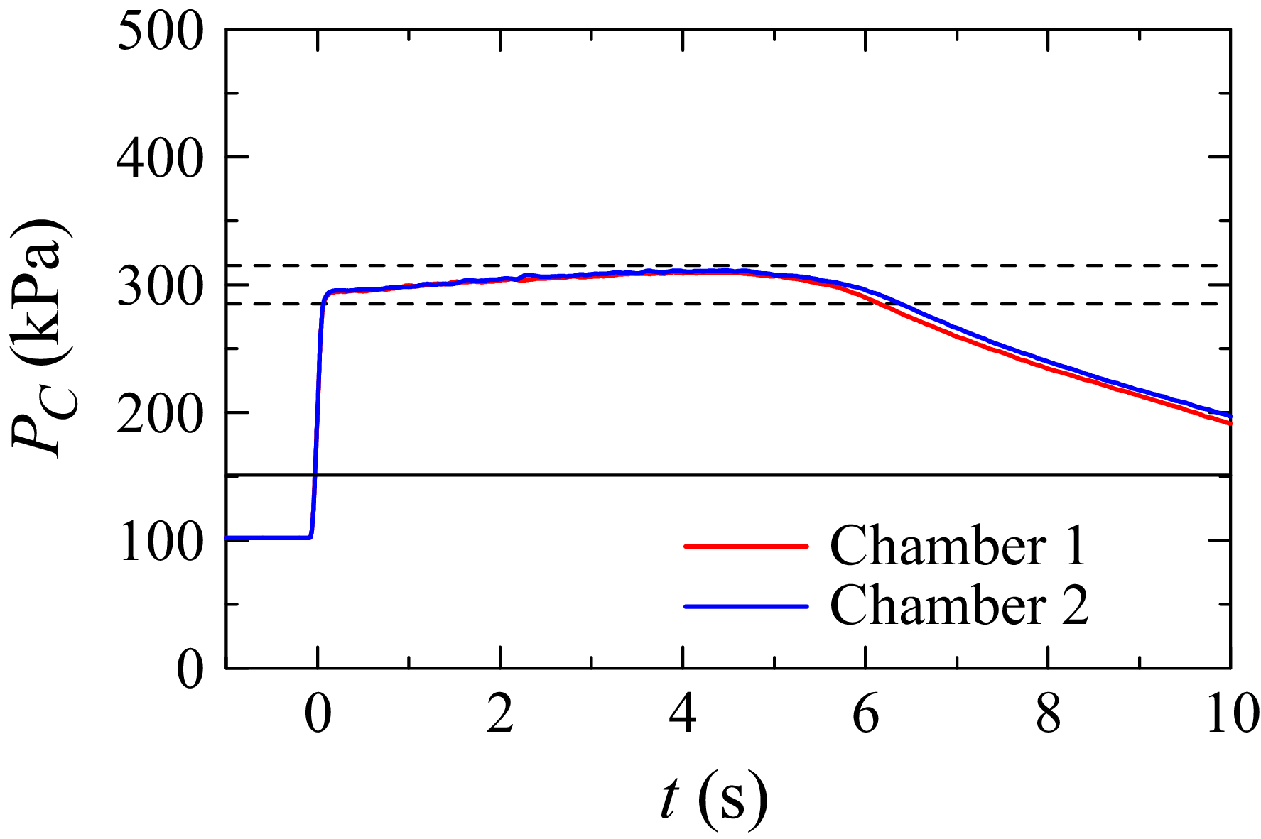
in the two chambers are measured simultaneously using pressure sensors (SMC, PSE540), and the signals are recorded with an oscilloscope (Yokogawa, DL850E) at 5 kHz. Figure 3 shows the pressure variation during a representative run. Immediately after valve opening, the pressure rises rapidly to
 $P_C \approx 300$
kPa. Up to
 $t \approx 5$
s, it continues to increase gradually due to the mechanical characteristics of the regulators, a phenomenon known as the supply pressure effect. The horizontal dashed lines indicate
 $\pm 5\,\%$
of 300 kPa. During the first 6 s, the pressure remains within this range. After
 $t \approx 6$
s, it decreases due to the pressure drop in the tanks. Accordingly, the flows are regarded as statistically steady during the initial 6 s, within which all measurements are conducted. The pressure difference between the two chambers remains negligible in this period, ensuring that both generators produce jets with the same characteristics. For the present nozzle design, the jet velocity at the nozzle outlet is independent of plenum pressure once it exceeds 151.2 kPa, as indicated by the horizontal solid line. The root-mean-square (r.m.s.) plenum-pressure fluctuation over the first 6 s is 7 kPa, which is sufficiently small that the jet velocity remains constant. Plenum-pressure fluctuations do, however, affect the static pressure and density at the nozzle outlet: for a 7 kPa fluctuation, both vary by about 2 %. These variations lead to 2 % fluctuations in the jet Reynolds number, indicating that jet properties hardly vary with time. This estimate is based on a one-dimensional nozzle-flow analysis and does not consider other effects such as wall influences inside the nozzle. Our previous study of the same jet array presented schlieren visualisation of the jet, which showed that the Mach disc forming from the nozzle outlet is steady in time (Mori et al. Reference Mori, Watanabe and Nagata2024). The visualisation also indicates small temporal variations in the jet properties.
Variations in plenum pressure
 $P_C$
in each plenum chamber. Horizontal dashed lines indicate
 $\pm 5\,\%$
of 300 kPa, for which the nozzles are designed to produce ideally expanded supersonic jets. The horizontal solid line denotes 151.2 kPa, the critical pressure above which the exit Mach number is independent of plenum pressure. The time origin (
 $t=0$
) corresponds to the instant when the pressure reaches 200 kPa. Signals are smoothed using a moving average with a window of 0.1 s.

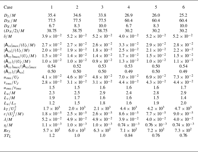
Table 1 lists the tested values of
 $D_I$
,
 $D_N$
and
 $D_E$
, together with measurement results discussed in § 3. These values are normalised by the jet spacing
 $M$
in table 1. Different geometric parameters are chosen to vary the characteristics of the strain and turbulence. Jet interaction forms nearly HIT, which decays in the mean flow direction within the inner duct (Mori et al. Reference Mori, Watanabe and Nagata2024). The inner-duct length
 $D_I$
is set to exceed
 $25M$
. The velocity fluctuations become statistically homogeneous in the cross-sectional plane before
 $25M$
downstream of the nozzles. As turbulence decays, the integral scale representing the characteristic size of large-scale motions increases. At large streamwise distances this growth leads to confinement effects from the test-section walls, manifested as accelerated decay of turbulent kinetic energy and inhibited scale growth (Skrbek & Stalp Reference Skrbek and Stalp2000; Morize & Moisy Reference Morize and Moisy2006), which become prominent beyond
 $50M$
(Watanabe et al. Reference Watanabe, Inagaki, Mori, Ishizawa and Nagata2025). Accordingly, the maximum
 $D_I$
is set below
 $50M$
. When the flows from the two generators reach the ends of the inner ducts, a stagnation point forms in the mean flow due to their interaction, with the mean velocity in the
 $x$
direction decreasing towards this point. Since the velocity gradient depends on the distance from the inner-duct end to the stagnation point, experiments are conducted with different gaps
 $D_E$
between
 $6.7M$
and
 $10.0M$
adjusted by varying
 $D_I$
according to
 $D_E=D_N-2D_I$
. Consequently, a small change in
 $D_I$
markedly affects
 $D_E$
: from case 5 to case 6,
 $D_I$
is reduced by about 3 %, leading to a 20 % increase in
 $D_E$
. Furthermore, as turbulence decays within the inner ducts, the properties at the test-section centre depend on the nozzle-to-centre distance
 $D_N/2$
. Tests with different
 $D_N$
values are therefore performed to vary the turbulence characteristics.
Experimental conditions and velocity statistics. Each case uses different test-section geometries defined in figure 2. The distance from the nozzle exit to the test-section centre is
 $D_N/2$
. The vector spacing in PIV is denoted by
 $\delta$
. The mean velocity gradient tensor is denoted by
 $\mathsf{A}_{\textit{ij}}=\partial \langle u_i\rangle /\partial x_{\!j}$
. The r.m.s. fluctuations of
 $u$
and
 $v$
are denoted by
 $u_{\textit{rms}}$
and
 $v_{\textit{rms}}$
, respectively. The integral scales of
 $u$
and
 $v$
are denoted by
 $L_u$
and
 $L_v$
and are obtained by integrating the corresponding longitudinal autocorrelation functions. A dissipation scaling is used to provide an order-of-magnitude estimate of the turbulent kinetic energy dissipation rate per unit mass,
 $\varepsilon =A\mathcal{U}^3/\mathcal{L}$
with
 $A=1$
, where
 $\mathcal{U}$
and
 $\mathcal{L}$
are the large-scale velocity and length scales. These are defined as
 $\mathcal{U}=\sqrt {2k_T/3}$
and
 $\mathcal{L}=(L_u+L_v+L_w)/3$
, where
 $k_T=(u_{\textit{rms}}^2+v_{\textit{rms}}^2+w_{\textit{rms}}^2)/2$
is the turbulent kinetic energy. We assume
 $w_{\textit{rms}}=v_{\textit{rms}}$
and
 $L_w=L_v$
for the r.m.s. fluctuation and integral scale of
 $w$
. The Taylor microscale and Kolmogorov scale are given by
 $\lambda =\sqrt {10(\mu /\rho )k_T/\varepsilon }$
and
 $\eta =(\mu /\rho )^{3/4}\varepsilon ^{-1/4}$
, respectively. The turbulent Reynolds number is
 $\textit{Re}_\lambda =\rho \sqrt {2k_T/3}\lambda /\mu$
. The table also includes
 $ST_L$
, which is the mean strain rate
 $S = (|\mathsf{A}_{\textit{xx}}| + 2\mathsf{A}_{\textit{yy}} + 2\mathsf{A}_{zz})/3$
with
 $\mathsf{A}_{zz}=\mathsf{A}_{\textit{yy}}$
normalised by the time scale of large-scale motions,
 $T_L$
. Most quantities are normalised by the jet velocity
 $U_{\!J}$
and the jet spacing
 $M$
. All statistics, except for
 $|\mathsf{A}_{\textit{xx}}|_{\textit{max}}$
and
 $(\mathsf{A}_{\textit{yy}})_{\textit{max}}$
, are evaluated as ensemble and spatial averages within the measurement region. Terms
 $|\mathsf{A}_{\textit{xx}}|_{\textit{max}}$
and
 $(\mathsf{A}_{\textit{yy}})_{\textit{max}}$
denote the maximum values of
 $|\mathsf{A}_{\textit{xx}}|$
and
 $\mathsf{A}_{\textit{yy}}$
, respectively.

2.3. Turbulence properties in single-jet-array experiments
Our previous studies employed the same jet generator in a turbulent wind tunnel (Mori et al. Reference Mori, Watanabe and Nagata2024; Watanabe et al. Reference Watanabe, Mori, Ishizawa and Nagata2024, Reference Watanabe, Inagaki, Mori, Ishizawa and Nagata2025). The tunnel had a 1 m long test section with a square cross-section of
 $100\times 100$
mm
 $^2$
. A
 $6\times 6$
array of jets was issued from one side of the test section, and their interaction generated nearly HIT decaying in the streamwise direction; the turbulent flow exited through the open downstream end. The jet nozzles and the test-section cross-sectional geometry were identical to those used in the present experiments, and the operating conditions were also the same. Velocity measurements were conducted with the same PIV system as employed here. Results from these single-jet-array studies are cited throughout this paper as a reference that approximates the initial turbulent state prior to the influence of mean strain for comparison with turbulence subject to axisymmetric expansion.
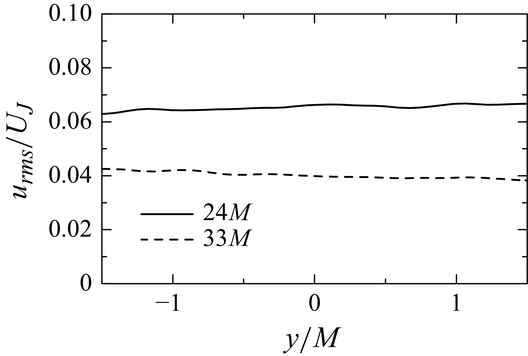
Figure 4 presents vertical profiles of the r.m.s. fluctuations of streamwise velocity
 $u$
,
 $u_{\textit{rms}}=\sqrt {\langle u^2\rangle -\langle u\rangle ^2}$
, computed from the PIV data in Mori et al. (Reference Mori, Watanabe and Nagata2024), where
 $\langle \ \ \rangle$
denotes ensemble averages of statistically independent samples. The profiles are shown at streamwise distances of
 $24M$
and
 $33M$
from the nozzles, slightly upstream of the inner-duct ends in the OMJA experiments. The results show that
 $u_{\textit{rms}}$
hardly depends on
 $y$
, indicating that the velocity fluctuations are statistically homogeneous in the cross-sectional planes.
Vertical profiles of r.m.s. streamwise velocity fluctuations,
 $u_{\textit{rms}}$
, at streamwise distances of
 $24M$
and
 $33M$
from the nozzles in the single-jet-array configuration. The PIV velocity data are taken from Mori et al. (Reference Mori, Watanabe and Nagata2024).

The turbulent Reynolds number is defined as
 $\textit{Re}_\lambda =\rho \sqrt {2k_T/3}\lambda /\mu$
, with the Taylor microscale
 $\lambda =\sqrt {10\mu k_T/(\rho \varepsilon )}$
and the turbulent kinetic energy
 $k_T$
. In the turbulent wind tunnel with the single jet array,
 $\textit{Re}_\lambda$
is about 600 at
 $38M$
and about 730 at
 $30M$
downstream of the nozzle array. These locations approximately correspond to the distance from the nozzles to the test-section centre,
 $D_N/2$
, in the OMJA experiments. The ratio of r.m.s. streamwise to vertical velocity fluctuations is about 1.08, close to values reported for grid turbulence (Krogstad & Davidson Reference Krogstad and Davidson2012; Isaza, Salazar & Warhaft Reference Isaza, Salazar and Warhaft2014; Kitamura et al. Reference Kitamura, Nagata, Sakai, Sasoh, Terashima, Saito and Harasaki2014 ). Thus, the degree of isotropy is similar to that of grid turbulence, which has been used to investigate changes in initially nearly isotropic turbulence under axisymmetric contraction (Hussain & Ramjee Reference Hussain and Ramjee1976; Sjögren & Johansson Reference Sjögren and Johansson1998; Ayyalasomayajula & Warhaft Reference Ayyalasomayajula and Warhaft2006; Ertunç & Durst Reference Ertunç and Durst2008; Alhareth et al. Reference Alhareth, Mugundhan, Langley and Thoroddsen2024).
2.4. Particle image velocimetry
Two-dimensional, two-component PIV is employed to investigate the turbulent flow field. Main measurements are conducted on the
 $x$
–
 $y$
plane at the centre of the test section (
 $z=0$
). For case 1, additional PIV measurements are conducted on the
 $x$
–
 $z$
plane at
 $y=0$
and on the
 $x$
–
 $y$
plane at
 $z=12$
mm to examine statistical axisymmetry. The set-up, including components, seeding method and post-processing tools, is identical to that used in our previous studies on the single jet array (Mori et al. Reference Mori, Watanabe and Nagata2024; Watanabe et al. Reference Watanabe, Mori, Ishizawa and Nagata2024). The PIV system consists of a double-pulse Nd:YAG laser (Dantec Dynamics, Dual Power 65-15), a high-speed camera (Dantec Dynamics, SpeedSense 9070) with
 $1280\times 800$
pixel resolution equipped with a macro lens (Nikon, AI AF Micro Nikkor 105 mm F2.8D) and a synchroniser (Dantec Dynamics, 80N77) controlling the camera and laser via integrated software (Dantec Dynamics, DynamicStudio). The laser head, positioned beneath the test section, illuminates the
 $x$
–
 $y$
plane through a reflecting mirror. For the
 $x$
–
 $z$
plane measurements, an additional mirror is used to illuminate the plane with the laser sheet entering from the side wall. A lens unit attached to the laser head produces a laser sheet thinner than 1 mm, with a pulse width of under 4 ns. The camera, mounted on a tripod and mechanically isolated from the OMJA facility, views the illuminated plane. The field of view (FOV) is centred at
 $x=0$
, equidistant from the two jet arrays. The FOV size is approximately
 $100 \times 60$
mm
 $^2$
for cases 2, 3, 5 and 6, and
 $75 \times 47$
mm
 $^2$
for cases 1 and 4. These sizes are equivalent to
 $8.3M\times 5.0M$
and
 $6.3M\times 3.9M$
, respectively. The smaller FOV in the latter cases results from obstruction by the test-section frame, as these involve a smaller inner-duct gap (
 $D_E \lt 100$
mm).
In line with previous studies of supersonic flows generated by Laval nozzles, the present PIV measurements employ condensed ethanol droplets as tracer particles (Clemens & Mungal Reference Clemens and Mungal1991; Pizzaia & Rossmann Reference Pizzaia and Rossmann2018; Kouchi et al. Reference Kouchi, Fukuda, Miyai, Nagata and Yanase2019; Mori et al. Reference Mori, Watanabe and Nagata2024). In these studies, droplets are generated by fluid expansion in Laval nozzles, using air with evaporated ethanol or acetone as working fluid. Prior to each experiment, absorbent fabric soaked with approximately 100 ml of liquid ethanol is affixed to the inner wall of each plenum chamber using a three-dimensional-printed stent. When the valves are opened, ethanol evaporates into the airflow through the plenum chambers, and the temperature drop in the Laval nozzles leads to condensation and droplet formation.
Condensation-generated tracers have very small diameters, making this seeding technique ideal for high-speed flows. Pizzaia & Rossmann (Reference Pizzaia and Rossmann2018) and Kouchi et al. (Reference Kouchi, Fukuda, Miyai, Nagata and Yanase2019) report ethanol/acetone droplet diameters of approximately
 $0.05$
–
 $0.2$
μm and
 $0.16$
μm, respectively. In our facility, Rayleigh scattering is clearly observed, consistent with droplet diameters smaller than the visible-light wavelength (360–830 nm) (Mori et al. Reference Mori, Watanabe and Nagata2024). Based on these observations, we evaluate the Stokes number using a particle diameter
 $d_p=0.2$
μm. The particle response time is
 $\tau _p=d_p^2\rho _p/18\mu =9.69\times 10^{-8}$
s, where
 $\rho _p=789$
kg m−3 is the ethanol density and
 $\mu =1.81\times 10^{-5}$
Pa s is the viscosity of air. We evaluate the turbulence time scale at
 $26M$
downstream from the nozzles based on PIV data for turbulence generated by the single jet array (Mori et al. Reference Mori, Watanabe and Nagata2024). The shortest turbulence time scale is the Kolmogorov time scale,
 $\tau _\eta =(\mu /\rho \varepsilon )^{1/2}=7.57\times 10^{-6}$
s. The corresponding Stokes number is
 $St=\tau _p/\tau _\eta =1.28\times 10^{-2}$
. Particles act as accurate tracers for
 $St\lt 0.1$
(Raffel et al. Reference Raffel, Willert, Scarano, Kähler, Wereley and Kompenhans2018), which is satisfied under the present experimental conditions.
Particle-image pairs are acquired at 15 Hz and processed in DynamicStudio using an adaptive PIV algorithm (Theunissen Reference Theunissen2010) combined with universal outlier detection (Westerweel & Scarano Reference Westerweel and Scarano2005). The interrogation window sizes vary between
 $16 \times 16$
and
 $32 \times 32$
pixels, with a vector spacing of 8 pixels. This corresponds to 50 % overlap for the minimum window and yields
 $159 \times 99$
velocity vectors per snapshot. The vector spacing, denoted by
 $\delta$
and normalised by the jet spacing
 $S$
, is summarised in table 1. For the present setting,
 $\delta /M\approx 0.04$
–
 $0.05$
is comparable to
 $\lambda$
and about
 $40\eta$
–
 $70\eta$
, as estimated in § 3.4. Thus, the measurements do not resolve the smallest scales of motion but are sufficient to capture large-scale properties such as mean velocity and r.m.s. fluctuations. The interval between successive laser pulses is adjusted between 3 and 6 μs to maintain an average particle displacement of about 2–3 pixels across different cases, where the particle displacement refers to the distance of particle movements between two particle images. This ensures that the average particle displacement is smaller than 1/4 of the interrogation window size and light-sheet thickness (Westerweel Reference Westerweel1997). For the current PIV algorithm, the subpixel accuracy is expected to be of order 0.02–0.05 pixels (Raffel et al. Reference Raffel, Willert, Scarano, Kähler, Wereley and Kompenhans2018). With the present pixel size of about 0.08 mm and the pulse interval, this corresponds to about 1 %–3 % of the r.m.s. velocity fluctuations. Under these settings for turbulence generated by a single jet array, our previous studies successfully recovered the Batchelor-type decay law, the
 $-5/3$
law of energy spectra, the exponential tail of longitudinal autocorrelation functions and the anomalous scaling of high-order moments of filtered velocity gradients (Mori et al. Reference Mori, Watanabe and Nagata2024; Watanabe et al. Reference Watanabe, Mori, Ishizawa and Nagata2024, Reference Watanabe, Inagaki, Mori, Ishizawa and Nagata2025). These comparisons with turbulence theory, experiments and DNS validate the present PIV measurements.
Measurements are repeated 12–13 times per case to obtain more than 1000 velocity snapshots. The acquired velocity vectors are further processed to evaluate statistical quantities. The characteristic time scale of large-scale turbulent motions, defined as the ratio of the integral length scale to the r.m.s. velocity fluctuation (see § 3.4), is less than 0.002 s, which is much shorter than the sampling interval of 0.067 s. Velocity vectors from two consecutive particle-image pairs are therefore considered statistically independent. Statistics are evaluated using ensemble averages of all snapshots. For a variable
 $f$
, its value in the
 $n$
th snapshot is denoted by
 $f^{(n)}$
. The ensemble average is given by
 \begin{align} \langle f\rangle = \frac {1}{N_S}\sum _{n=1}^{N_S} f^{(n)}, \end{align}
as a function of positions, where
 $N_S$
is the total number of snapshots. Velocity components
 $(u,v,w)$
are decomposed into mean and fluctuating parts, with fluctuations denoted by
 $u'=u-\langle u\rangle$
,
 $v'=v-\langle v\rangle$
and
 $w'=w-\langle w\rangle$
. The r.m.s. fluctuations are defined as
 $u_{\textit{rms}} = \langle {u'}^2 \rangle ^{1/2}$
,
 $v_{\textit{rms}} = \langle {v'}^2 \rangle ^{1/2}$
and
 $w_{\textit{rms}}= \langle {w'}^2 \rangle ^{1/2}$
. Other velocity statistics are defined when they are introduced.
A spatial smoothing filter, implemented as a moving average, is applied to ensemble-averaged fields when presenting contour plots to highlight spatial distributions. Additionally, spatial averages within the FOV are used to describe bulk turbulence properties. Statistical uncertainties from finite sampling are estimated by dividing the dataset into two subsets; the r.m.s. differences between their statistics are shown as error bars in the results below.
2.5. Temperature and pressure measurements
In addition to PIV, supplemental experiments are conducted to measure temperature and static pressure at the centre of the test section to determine fluid properties required for evaluating the local Reynolds number and length scales. The methods follow those in our previous study using the same jet generator (Mori et al. Reference Mori, Watanabe and Nagata2024). Temperature is measured with a fine-sheathed K-type thermocouple (J Thermo, TJK-LS1501GP) of 0.15 mm sheath diameter, 100 mm length and a response time under 1 s. The thermocouple, supported by a stainless steel rod with thermal insulation, is inserted through closable holes in the top wall of the outer duct. The output voltage is processed and recorded by a data logger (Hioki, LR8431) with internal calibration at a sampling rate of 100 Hz. The mean temperature
 $T$
is evaluated as the time average over 6 s and ensemble average of three runs. At the test-section centre, the mean temperature is approximately
 $290 \pm 2$
K under all conditions.
Static pressure is measured using the static port of an L-shaped standard Pitot tube (Testo, 0635 2145) connected to a pressure sensor (SMC, PSE543A). The analogue output of the sensor is recorded by an oscilloscope (Yokogawa, DL850E) at a sampling rate of 10 kHz. The Pitot tube is inserted from the top of the outer duct, in the same manner as the thermocouple. At the test-section centre, the mean gauge pressure is approximately
 $10^2$
PaG, much smaller than atmospheric pressure.
Based on the measured mean temperature
 $T$
and pressure
 $P$
, the density
 $\rho$
is evaluated from the equation of state,
 $P = \rho R T$
, with the gas constant
 $R = 287$
J (kg K)−1. The viscosity
 $\mu$
is determined using Sutherland’s law:
 \begin{align} \mu = \mu _0 \left (\frac {T}{T_0}\right )^{3/2}\frac {T_0 + S_\mu }{T + S_\mu }, \end{align}
where
 $T_0 = 273$
K is the reference temperature,
 $S_\mu = 110.4$
K is the Sutherland constant and
 $\mu _0 = 1.724 \times 10^{-5}$
Pa s is the reference viscosity.
Pressure and temperature measurements at the test-section centre yield density
 $\rho =1.25$
kg m−
 $^{3}$
, viscosity
 $\mu =1.81\times 10^{-5}$
Pa s and kinematic viscosity
 $\nu =\mu /\rho =1.44\times 10^{-5}$
m
 $^2$
s−1. These values do not vary among the different test-section geometries.
3. Results and discussion
3.1. Mean flow field
Figure 5 presents the mean flow field for each case, showing mean velocity streamlines and a colour contour of the magnitude of the mean velocity vector,
 $|\langle {\boldsymbol{u}}\rangle |$
. The streamlines indicate that opposing flows approach from both sides along the
 $x$
direction and expand vertically near the test-section centre. The stagnation point is identified by the minimum value of
 $|\langle {\boldsymbol{u}}\rangle |$
, close to zero, and is marked by red crosses. In all cases, the stagnation point is located near the geometric centre of the test section,
 $(x,y)=(0,0)$
, owing to the symmetric configuration of the test section and jet arrays. The streamline patterns imply
 $\partial \langle u \rangle /\partial x \lt 0$
and
 $\partial \langle v \rangle /\partial y \gt 0$
, consistent with axisymmetric expansion described by (1.3). The mean velocity remains below 45 m s−1 in all cases, implying that the mean flow Mach number is less than 0.3.
Averaged velocity fields coloured by the mean velocity magnitude,
 $|\langle \boldsymbol{u}\rangle |=\sqrt {\langle u\rangle ^2+\langle v\rangle ^2}$
, on the
 $x$
–
 $y$
plane at
 $z=0$
. Black lines with arrows indicate streamlines. Red crosses denote the minimum value of
 $|\langle \boldsymbol{u}\rangle |$
. Panels show results for different test section geometries: (
 $a$
) case 1, (
 $b$
) case 2, (
 $c$
) case 3, (
 $d$
) case 4, (
 $e$
) case 5 and (
 $f$
) case 6.

Figure 6 visualises the mean flow on the
 $x$
–
 $z$
plane at
 $y=0$
and on the
 $x$
–
 $y$
plane at
 $z/M=1$
. Owing to the geometry of the test section and jet arrays, the
 $x$
–
 $z$
plane at
 $y=0$
is equivalent to the
 $x$
–
 $y$
plane at
 $z=0$
. The mean velocity pattern of axisymmetric expansion is visible on the
 $x$
–
 $z$
plane as well as on the off-centre
 $x$
–
 $y$
plane.
Averaged velocity fields coloured by the mean velocity magnitude in case 1: (
 $a$
)
 $|\langle \boldsymbol{u}\rangle |=\sqrt {\langle u\rangle ^2+\langle w\rangle ^2}$
on the
 $x$
–
 $z$
plane at
 $y=0$
; (
 $b$
)
 $|\langle \boldsymbol{u}\rangle |=\sqrt {\langle u\rangle ^2+\langle v\rangle ^2}$
on the
 $x$
–
 $y$
plane at
 $z/M=1$
. Black lines with arrows indicate streamlines. Red crosses denote the minimum value of
 $|\langle \boldsymbol{u}\rangle |$
.

The mean velocity gradients associated with axisymmetric strain are given by the diagonal components of
 ${\unicode{x1D63C}}$
in (1.1), namely
 $\mathsf{A}_{\textit{xx}} = \partial \langle u \rangle /\partial x$
,
 $\mathsf{A}_{\textit{yy}} = \partial \langle v \rangle /\partial y$
and
 $\mathsf{A}_{zz} = \partial \langle w \rangle /\partial z$
. Since central-difference approximations introduce significant errors due to statistical uncertainty in the mean velocity distribution, the gradients are instead obtained by fitting
 $\langle u \rangle$
,
 $\langle v \rangle$
and
 $\langle w \rangle$
with bicubic functions
 $(x,y)$
or
 $(x,z)$
. This choice is motivated by the observation that a third-order polynomial adequately captures one-dimensional profiles of mean velocities along either
 $x$
,
 $y$
or
 $z$
axis. Higher-order functions were also tested but offered no improvement in accuracy and instead introduced unnecessary complexity and the risk of over-fitting.
Figures 7 and 8 show colour contours of
 $|\mathsf{A}_{\textit{xx}}|$
and
 $\mathsf{A}_{\textit{yy}}$
, normalised by their respective maxima
 $|\mathsf{A}_{\textit{xx}}|_{\textit{max}}$
and
 $(\mathsf{A}_{\textit{yy}})_{\textit{max}}$
. In all cases,
 $|\mathsf{A}_{\textit{xx}}|$
and
 $\mathsf{A}_{\textit{yy}}$
decrease with increasing
 $|x|$
, indicating that the mean strain strengthens as the flow enters the gap between the inner ducts and approaches the test-section centre. At
 $x \approx 0$
, both
 $|\mathsf{A}_{\textit{xx}}|$
and
 $\mathsf{A}_{\textit{yy}}$
increase with
 $|y|$
in cases 1–3, but the dependence on
 $x$
is stronger than on
 $y$
.
Distributions of the mean velocity gradient magnitude
 $|\mathsf{A}_{\textit{xx}}|$
normalised by its maximum value
 $|\mathsf{A}_{\textit{xx}}|_{\textit{max}}$
. Panels show results for different test-section geometries: (
 $a$
) case 1, (
 $b$
) case 2, (
 $c$
) case 3, (
 $d$
) case 4, (
 $e$
) case 5 and (
 $f$
) case 6.

Same as figure 7, but for
 $\mathsf{A}_{\textit{yy}}$
normalised by
 $(\mathsf{A}_{\textit{yy}})_{\textit{max}}$
: (
 $a$
) case 1, (
 $b$
) case 2, (
 $c$
) case 3, (
 $d$
) case 4, (
 $e$
) case 5 and (
 $f$
) case 6.

Table 1 includes the maximum values of
 $|\mathsf{A}_{\textit{xx}}|$
in each case. The mean velocity in the
 $x$
direction decreases from that in the inner duct to nearly zero at the stagnation point, and when
 $D_E$
is large this decrease occurs over a longer distance. Consequently, the mean velocity gradient tends to be smaller for larger
 $D_E$
. For fixed
 $D_N$
,
 $|\mathsf{A}_{\textit{xx}}|_{\textit{max}}$
decreases with increasing
 $D_E$
, but variations in
 $D_N$
also affect
 $|\mathsf{A}_{\textit{xx}}|_{\textit{max}}$
, indicating that it is not determined solely by
 $D_E$
.
A key feature of axisymmetric expansion is the ratio of the diagonal velocity gradients, satisfying
 $\mathsf{A}_{\textit{yy}} = \mathsf{A}_{zz} = -\mathsf{A}_{\textit{xx}}/2 \gt 0$
. Figure 9 shows the distribution of
 $-\mathsf{A}_{\textit{yy}}/\mathsf{A}_{\textit{xx}}$
on the
 $x$
–
 $y$
plane at
 $z=0$
. Deviations from
 $-\mathsf{A}_{\textit{yy}}/\mathsf{A}_{\textit{xx}}=0.5$
are observed only near the edges of the measurement region. In most regions close to the test-section centre,
 $-\mathsf{A}_{\textit{yy}}/\mathsf{A}_{\textit{xx}}$
is close to
 $0.5$
, lying within the range 0.4–0.6. Figure 10(
 $a$
) presents the distribution of
 $-\mathsf{A}_{zz}/\mathsf{A}_{\textit{xx}}$
measured on the
 $x$
–
 $z$
plane at
 $y=0$
in case 1. As with
 $-\mathsf{A}_{\textit{yy}}/\mathsf{A}_{\textit{xx}}$
,
 $-\mathsf{A}_{zz}/\mathsf{A}_{\textit{xx}}$
is close to 0.5 except near the edges of the measurement region. Taken together,
 $-\mathsf{A}_{\textit{yy}}/\mathsf{A}_{\textit{xx}}\approx -\mathsf{A}_{zz}/\mathsf{A}_{\textit{xx}}\approx 0.5$
provides direct evidence of the formation of axisymmetric expansion and suggests that the continuity equation for the mean velocity in an incompressible flow is satisfied without compressibility effects. This is also consistent with the subsonic mean velocity, as low as about 45 m s−1. Figure 10(
 $b$
) shows the distribution of
 $-\mathsf{A}_{\textit{yy}}/\mathsf{A}_{\textit{xx}}$
on the
 $x$
–
 $y$
plane at
 $z/M=1$
in case 1. Even on this off-centre plane,
 $-\mathsf{A}_{\textit{yy}}/\mathsf{A}_{\textit{xx}}\approx 0.5$
holds except near the edges of the measurement region. These results demonstrate that axisymmetric strain is broadly established in the gap between the inner ducts of the two jet generators.
Distributions of the ratio of mean velocity gradients,
 $-\mathsf{A}_{\textit{yy}}/\mathsf{A}_{\textit{xx}}$
. Panels show results for different test-section geometries: (
 $a$
) case 1, (
 $b$
) case 2, (
 $c$
) case 3, (
 $d$
) case 4, (
 $e$
) case 5 and (
 $f$
) case 6.

Distributions of (
 $a$
)
 $-\mathsf{A}_{zz}/\mathsf{A}_{\textit{xx}}$
on the
 $x$
–
 $z$
plane at
 $y=0$
and (
 $b$
)
 $-\mathsf{A}_{\textit{yy}}/\mathsf{A}_{\textit{xx}}$
on the
 $x$
–
 $y$
plane at
 $z/M=1$
in case 1.

Table 1 lists the maximum values of
 $|\mathsf{A}_{\textit{xx}}|$
and
 $\mathsf{A}_{\textit{yy}}$
, denoted by
 $|\mathsf{A}_{\textit{xx}}|_{\textit{max}}$
and
 $(\mathsf{A}_{\textit{yy}})_{\textit{max}}$
, together with spatially averaged values of
 $|\mathsf{A}_{\textit{xx}}|$
and
 $\mathsf{A}_{\textit{yy}}$
. The ratios
 $(\mathsf{A}_{\textit{yy}})_{\textit{max}}/|\mathsf{A}_{\textit{xx}}|_{\textit{max}}$
and
 $\mathsf{A}_{\textit{yy}}/|\mathsf{A}_{\textit{xx}}|$
are also shown, both close to 1/2. Using the incompressible continuity equation,
 $\mathsf{A}_{zz}$
is estimated as
 $\mathsf{A}_{zz} = -\mathsf{A}_{\textit{xx}} - \mathsf{A}_{\textit{yy}}$
, which yields
 $\mathsf{A}_{\textit{yy}} \approx \mathsf{A}_{zz}$
when
 $\mathsf{A}_{\textit{yy}} \approx -\mathsf{A}_{\textit{xx}}/2$
. Thus, the condition for axisymmetric expansion is satisfied for both maximum and average values. Moreover, the relation
 $\mathsf{A}_{\textit{yy}} \approx \mathsf{A}_{zz}$
indicates that the flow is statistically axisymmetric in the
 $y$
and
 $z$
directions.
In summary, all cases successfully produce a mean strain characterised by compression in the
 $x$
direction and expansion in the
 $y$
and
 $z$
directions. Axisymmetric expansion, with
 $\mathsf{A}_{\textit{xx}} : \mathsf{A}_{\textit{yy}} : \mathsf{A}_{zz} = -2 : 1 : 1$
, is broadly observed near the test-section centre. This condition is uniformly satisfied for
 $|x/M| \leqslant 3$
and
 $|y/M| \leqslant 1.5$
. Although
 $-\mathsf{A}_{\textit{yy}}/\mathsf{A}_{\textit{xx}}$
remains approximately constant, both
 $-\mathsf{A}_{\textit{xx}}$
and
 $\mathsf{A}_{\textit{yy}}$
exhibit spatial variations, such that the strain rate intensifies as the flow approaches the test-section centre in the
 $x$
direction. Similar non-uniformity of axisymmetric strain has often been reported in wind tunnel experiments with variable cross-sections (Ayyalasomayajula & Warhaft Reference Ayyalasomayajula and Warhaft2006). The relation
 $\mathsf{A}_{\textit{yy}} = \mathsf{A}_{zz}$
, implied by the continuity equation, indicates statistical axisymmetry in the
 $y$
and
 $z$
directions, consistent with the symmetry of the test section and jet generators. Importantly,
 $-\mathsf{A}_{\textit{xx}}/2 = \mathsf{A}_{\textit{yy}} = \mathsf{A}_{zz}$
is satisfied not only along the symmetry axis (
 $y=0$
) but also for
 $y \neq 0$
and
 $z \neq 0$
, demonstrating that the mean strain remains axisymmetric throughout the central region of the test section. This mean strain characterisation provides the basis for interpreting the turbulence statistics discussed below.
3.2. One-point statistics of velocity fluctuations
One-point statistics of velocity fluctuations are evaluated to characterise the turbulence properties under axisymmetric expansion. Table 1 reports the spatially averaged values of
 $u_{\textit{rms}}$
and
 $v_{\textit{rms}}$
for all cases. Cases 1–3 exhibit lower values of
 $u_{\textit{rms}}$
and
 $v_{\textit{rms}}$
than cases 4–6. The turbulence generated by jet interaction decays within the inner duct. Since cases 1–3 employ longer inner ducts, the turbulence decays more before reaching the test-section centre, leading to smaller r.m.s. velocity fluctuations in the region where the mean strain forms. The present experiments test three values of the distance
 $D_E$
between the ends of the two inner ducts. However, the r.m.s. velocity fluctuations are less sensitive to
 $D_E$
than to
 $D_N$
. In all cases,
 $u_{\textit{rms}}$
exceeds
 $v_{\textit{rms}}$
, indicating anisotropy. Turbulence generated by the single jet array exhibits
 $u_{\textit{rms}}/v_{\textit{rms}} \approx 1.08$
(Mori et al. Reference Mori, Watanabe and Nagata2024). In the present experiments, the nearly HIT generated by jet interaction experiences axisymmetric expansion near the test-section centre, resulting in anisotropic velocity fluctuations. Table 1 also includes
 $u_{\textit{rms}}/v_{\textit{rms}}$
values evaluated from spatial averages of
 $u_{\textit{rms}}$
and
 $v_{\textit{rms}}$
. This ratio exceeds 1.4, much larger than the value of 1.08 for turbulence without axisymmetric expansion. Direct numerical simulations of initially isotropic turbulence subject to axisymmetric expansion have also shown that
 $u_{\textit{rms}}/v_{\textit{rms}} \gt 1$
(Lee Reference Lee1989), even though the turbulent Reynolds number, estimated in § 3.4, is much larger in the present experiments. Thus, the observed increase in
 $u_{\textit{rms}}/v_{\textit{rms}}$
due to axisymmetric expansion is consistent with previous numerical results.
Figures 11 and 12 show the distributions of
 $u_{\textit{rms}}$
and
 $v_{\textit{rms}}$
on the
 $x$
–
 $y$
plane at
 $z=0$
. The colour contours indicate relative deviations from the spatially averaged value in the FOV,
 $F_{{avg}}$
, defined as
 $\Delta (F)=(F-F_{{avg}})/F_{{avg}}$
for
 $F=u_{\textit{rms}}$
or
 $v_{\textit{rms}}$
. In figure 11,
 $u_{\textit{rms}}$
increases towards
 $x=0$
from both sides, whereas
 $v_{\textit{rms}}$
shows little dependence on
 $x$
for cases 1–3 and decreases to the centre for cases 4–6. Turbulence begins to be influenced by the mean strain near the ends of the inner ducts. As it is advected by the mean flow towards the test-section centre, it is exposed to the mean strain for a longer time. Additionally, the mean strain intensifies towards the test-section centre. This combination of strain intensification and accumulation of strain effects likely contributes to the increase in
 $u_{\textit{rms}}$
near the test-section centre. In contrast, variations in
 $v_{\textit{rms}}$
in the same region are less pronounced. Results of DNS studies of turbulence subject to axisymmetric strain at low Reynolds numbers have shown that the strain exerts stronger influence on r.m.s. velocity fluctuations in the symmetry axis direction, here the
 $x$
direction, than in the lateral (
 $y$
and
 $z$
) directions (Lee Reference Lee1989). These numerical findings qualitatively agree with the greater changes in
 $u_{\textit{rms}}$
observed toward the test-section centre.
Relative difference of r.m.s. velocity fluctuations in the
 $x$
direction,
 $u_{\textit{rms}}$
, from the spatially averaged value
 $(u_{\textit{rms}})_{{avg}}$
, defined as
 $\Delta (u_{\textit{rms}}) = [u_{\textit{rms}} - (u_{\textit{rms}})_{{avg}}]/(u_{\textit{rms}})_{{avg}}$
, on the
 $x$
–
 $y$
plane at
 $z=0$
. Here the subscript ‘avg’ denotes spatial averages within the FOV. Panels show results for different test-section geometries: (
 $a$
) case 1, (
 $b$
) case 2, (
 $c$
) case 3, (
 $d$
) case 4, (
 $e$
) case 5 and (
 $f$
) case 6.

Same as figure 11, but for r.m.s. velocity fluctuations in the
 $y$
direction,
 $v_{\textit{rms}}$
: (
 $a$
) case 1, (
 $b$
) case 2, (
 $c$
) case 3, (
 $d$
) case 4, (
 $e$
) case 5 and (
 $f$
) case 6. The relative difference is defined as
 $\Delta (v_{\textit{rms}}) = [v_{\textit{rms}} - (v_{\textit{rms}})_{{avg}}]/(v_{\textit{rms}})_{{avg}}$
.

Under axisymmetric expansion with
 $\mathsf{A}_{\textit{xx}}=-2\mathsf{A}_{\textit{yy}}=-2\mathsf{A}_{zz}\lt 0$
, the production term of turbulent kinetic energy of the
 $\alpha$
-directional velocity component is written as
 $P_\alpha =-\langle {u^{\prime}_\alpha }^2\rangle \mathsf{A}_{\alpha \alpha }$
with
 $\alpha =x,\ y$
or
 $z$
, where no summation is applied over
 $\alpha$
(Nieuwstadt et al. Reference Nieuwstadt, Westerweel and Boersma2016). This gives
 $P_x\gt 0$
and
 $P_y=P_z\lt 0$
, indicating an increase in the streamwise and a decrease in the transverse velocity fluctuations. Moreover, when turbulence is initially isotropic with
 $\langle {u'}^2\rangle =\langle {v'}^2\rangle =\langle {w'}^2\rangle$
, the relation
 $\mathsf{A}_{\textit{xx}}:\mathsf{A}_{\textit{yy}}:\mathsf{A}_{zz}=-2:1:1$
yields
 $P_x=2|P_y|=2|P_z|$
, implying that the strain induces greater changes to the velocity fluctuations in the
 $x$
direction than in the transverse (
 $y$
and
 $z$
) directions. Consistently, a significant increase in
 $u_{\textit{rms}}$
towards the test-section centre is observed in figure 11. These explanations are also consistent with DNS and RDT results (Lee Reference Lee1989). For axisymmetric contraction, the signs of
 $P_\alpha$
are reversed; transverse velocity fluctuations are amplified and longitudinal fluctuations attenuated, resulting in a decrease in
 $u_{\textit{rms}}/v_{\textit{rms}}$
(Lee Reference Lee1989; Ayyalasomayajula & Warhaft Reference Ayyalasomayajula and Warhaft2006).
Figure 13 compares
 $v_{\textit{rms}}$
and
 $w_{\textit{rms}}$
along the
 $x$
direction at the test-section centre,
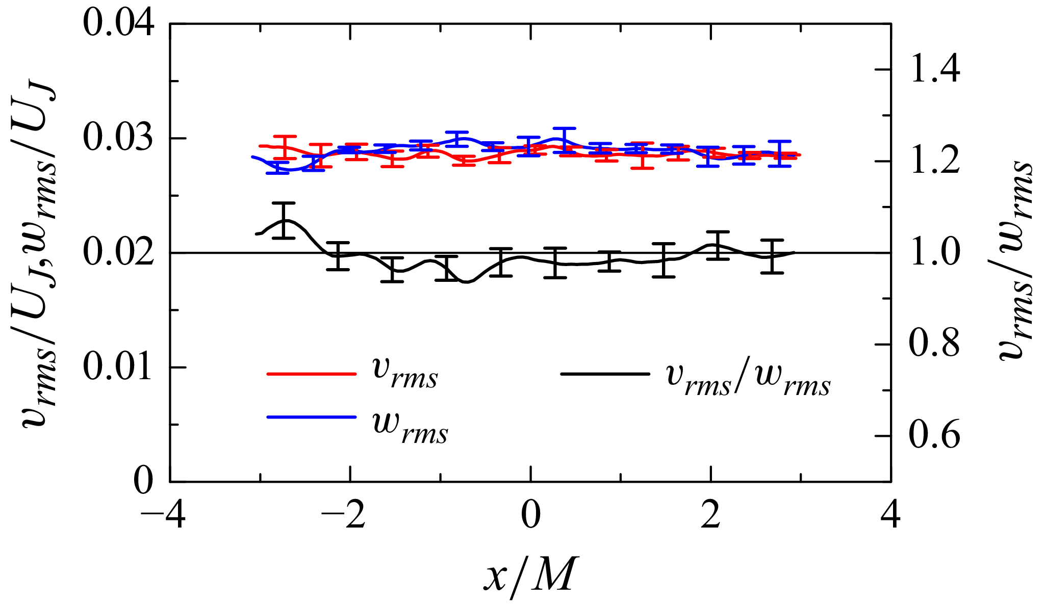
 $(y,z)=(0,0)$
, for case 1. These components exhibit similar r.m.s. levels, as indicated by
 $v_{\textit{rms}}/w_{\textit{rms}}\approx 1$
, which is required for statistical axisymmetry. This also follows from the geometry of the test section and jet arrays, which are identical in the
 $y$
and
 $z$
directions.
The
 $x$
-directional distributions of r.m.s. velocity fluctuations in the
 $y$
and
 $z$
directions,
 $v_{\textit{rms}}$
and
 $w_{\textit{rms}}$
, and their ratio
 $v_{\textit{rms}}/w_{\textit{rms}}$
at
 $(y,z)=(0,0)$
in case 1.

Statistical axisymmetry in the present set-up requires that, at a given
 $x$
, velocity statistics depend solely on
 $r_{yz}=\sqrt {y^2+z^2}$
and are independent of the azimuthal angle
 $\theta =\tan ^{-1}(y/z)$
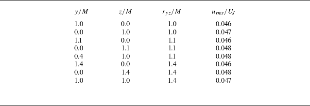
. Table 2 compares
 $u_{\textit{rms}}$
at the same
 $r_{yz}$
but at different
 $(y,z)$
locations at
 $x=0$
on three measurement planes: the
 $x$
–
 $y$
planes at
 $z/M=0$
and 1 and the
 $x$
–
 $z$
plane at
 $y=0$
. For
 $r_{yz}/M=1$
, two points are presented because the locations at this
 $r_{yz}$
on the
 $x$
–
 $y$
plane at
 $z/M=1$
and the
 $x$
–
 $z$
plane at
 $y=0$
are identical. Although the square cross-section and square nozzle arrangement could, in principle, introduce
 $\theta$
dependence,
 $u_{\textit{rms}}$
at the same
 $r_{yz}$
shows no significant variation across
 $(y,z)$
locations. Therefore, the square geometries do not introduce
 $\theta$
dependence near the test-section centre.
Radial variations of
 $u_{\textit{rms}}$
at different azimuthal locations at
 $x=0$
in case 1.

Large-scale anisotropy is often characterised using the normalised anisotropy tensor of Reynolds stress (Pope Reference Pope2000), defined as
 \begin{align} \mathsf{b}_{\textit{ij}} = \frac {\langle u^{\prime}_i u^{\prime}_{\!j}\rangle }{\langle u^{\prime}_k u^{\prime}_k\rangle } - \frac {1}{3} \delta _{\textit{ij}}, \end{align}
where the summation convention is applied to repeated indices,
 $i,j,k=x,y$
or
 $z$
, and
 $\delta _{\textit{ij}}$
is the Kronecker delta. Second and third invariants of
 $\mathsf{b}_{\textit{ij}}$
, denoted by
 $B_2$
and
 $B_3$
, are given by
 $B_2 = (\mathsf{b}_{\textit{ij}} \mathsf{b}_{ji}/6)^{1/2}$
and
 $B_3 = (\mathsf{b}_{\textit{ij}} \mathsf{b}_{jk} \mathsf{b}_{ki}/6)^{1/3}$
. Anisotropy states are commonly visualised using a plot of
 $(B_2, B_3)$
, known as the Lumley triangle. The PIV measurements of
 $(u,v)$
on the
 $x$
–
 $y$
plane provide
 $\mathsf{b}_{\textit{xx}}$
,
 $\mathsf{b}_{\textit{yy}}$
and
 $\mathsf{b}_{xy}=\mathsf{b}_{yx}$
. Based on the assumption of axisymmetry at
 $(y,z)=(0,0)$
, the following conditions are adopted in the analysis of
 $B_2$
and
 $B_3$
:
 $\mathsf{b}_{\textit{yy}}=\mathsf{b}_{zz}$
and
 $\mathsf{b}_{\textit{ij}}=0$
for
 $i\neq j$
. The present PIV yields
 $|\langle u'v'\rangle |/u_{\textit{rms}}v_{\textit{rms}}\lt 0.1$
at
 $(y,z)=(0,0)$
for all cases, indicating that
 $\mathsf{b}_{\textit{ij}}$
with
 $i\neq j$
is sufficiently small. These simplifications for axisymmetric expansion yield
 $B_2=B_3$
. Accordingly, this study examines the spatial distribution of
 $B_2$
. The omission of
 $\mathsf{b}_{12}$
and
 $\mathsf{b}_{21}$
has negligible effect, as their inclusion hardly alters
 $B_2$
values. For isotropic turbulence,
 $B_2=0$
. As the flow departs from isotropy under axisymmetric expansion,
 $B_2=B_3$
increases, with the theoretical upper bound of
 $1/3$
attained when
 $\langle u^{\prime 2}\rangle \gg \langle v^{\prime 2}\rangle =\langle w^{\prime 2}\rangle$
.
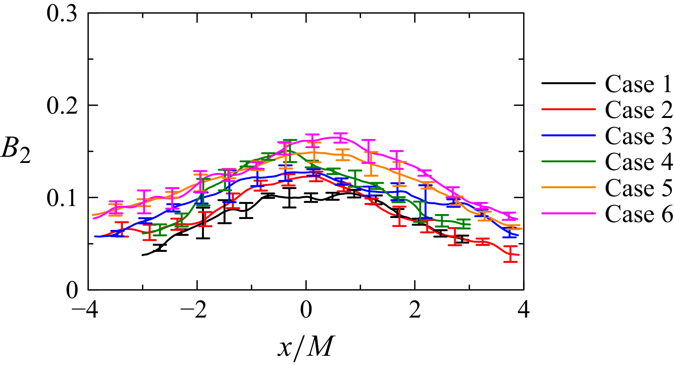
Figure 14 shows the
 $x$
-directional distribution of
 $B_2$
at
 $(y,z)=(0,0)$
. Nearly HIT generated by the single jet array exhibits
 $B_2 \approx 0.03$
(Mori et al. Reference Mori, Watanabe and Nagata2024). In contrast, the present experimental set-up yields higher
 $B_2$
values, indicating that the flow becomes anisotropic. For all cases,
 $B_2$
increases from both sides towards the test-section centre, demonstrating that anisotropy intensifies as the fluid subjected to the mean strain is advected with the mean flow. This increasing trend of
 $B_2$
is observed consistently across all test-section geometries.
The
 $x$
-directional distribution of the invariant
 $B_2$
of the normalised anisotropy tensor
 $\mathsf{b}_{\textit{ij}}$
along the centreline,
 $(y,z)=(0,0)$
.

Figure 15 presents the profiles of skewness and flatness of
 $u$
, defined as
 $S_u=\langle {u'}^3\rangle /\langle {u'}^2\rangle ^{3/2}$
and
 $F_u=\langle {u'}^4\rangle /\langle {u'}^2\rangle ^{2}$
. For Gaussian velocity fluctuations,
 $S_u=0$
and
 $F_u=3$
. Deviations from these values typically indicate large-scale intermittency, i.e. intermittency of energy-containing motions (Veeravalli & Warhaft Reference Veeravalli and Warhaft1989; Davidson Reference Davidson2015). This differs from small-scale intermittency, which refers to the burstiness of small-scale motions, typically evident in velocity-gradient statistics. Large-scale intermittency is observed in turbulent free-shear flows (e.g. jets and wakes) and other inhomogeneous turbulent flows, where the presence and absence of large coherent structures alternate at a fixed point. In such cases, the magnitudes of skewness and flatness can reach values as large as
 $1$
and
 $5$
, respectively (Kang & Meneveau Reference Kang and Meneveau2008; Matsushima, Nagata & Watanabe Reference Matsushima, Nagata and Watanabe2021; Nakamura et al. Reference Nakamura, Matsushima, Zheng, Nagata and Watanabe2022, Reference Nakamura, Watanabe and Nagata2023). In the present measurements,
 $|S_u|$
remains below 0.3 and
 $F_u$
is close to 3 near the test-section centre, showing that large-scale intermittency is negligible in this region. While
 $F_u$
tends to exceed 3 as
 $|x|$
increases, suggesting slight intermittency in the flow entering the gap region from the inner duct ends, the deviation remains moderate and far smaller than that in flows with pronounced large-scale intermittency.
Distributions of (
 $a$
) skewness
 $S_u$
and (
 $b$
) flatness
 $F_u$
of
 $x$
-directional velocity fluctuations along the centreline,
 $(y,z)=(0,0)$
.

3.3. Two-point statistics and energy spectra
We examine two-point statistics and energy spectra from PIV on the
 $x$
–
 $y$
plane at
 $z=0$
to evaluate integral length scales and the scale dependence of velocity fluctuations, using autocorrelation functions, energy spectra and structure functions. For evaluating these quantities, spatial averages in the
 $x$
and
 $y$
directions are taken over
 $|x|\lt 2M$
and
 $|y|\lt M$
, respectively, thereby excluding corner regions where the mean velocity gradients depart from axisymmetric strain.
Large-scale properties are examined using the longitudinal autocorrelation functions of velocity fluctuations at two points separated by a distance
 $r$
, defined as
 \begin{align} f_{u}(r,x,y) &= \frac {\langle u'(x - r/2, y) u'(x + r/2, y)\rangle }{\langle u^{\prime 2}(x, y)\rangle }, \end{align}
 \begin{align} f_{v}(r,x,y) &= \frac {\langle v'(x, y - r/2) v'(x, y + r/2)\rangle }{\langle v^{\prime 2}(x, y)\rangle }. \end{align}
These functions are used to estimate the integral length scale, which characterises large-scale motions. The symmetric forms of the autocorrelation functions, i.e. correlations between
 $x+r/2$
and
 $x-r/2$
rather than between
 $x$
and
 $x+r$
, are used to evaluate turbulent properties at a given point because the flow is statistically inhomogeneous. Here,
 $f_u$
is evaluated at
 $x=0$
and
 $f_v$
at
 $y=0$
with spatial averaging applied in the
 $y$
and
 $x$
directions, respectively.
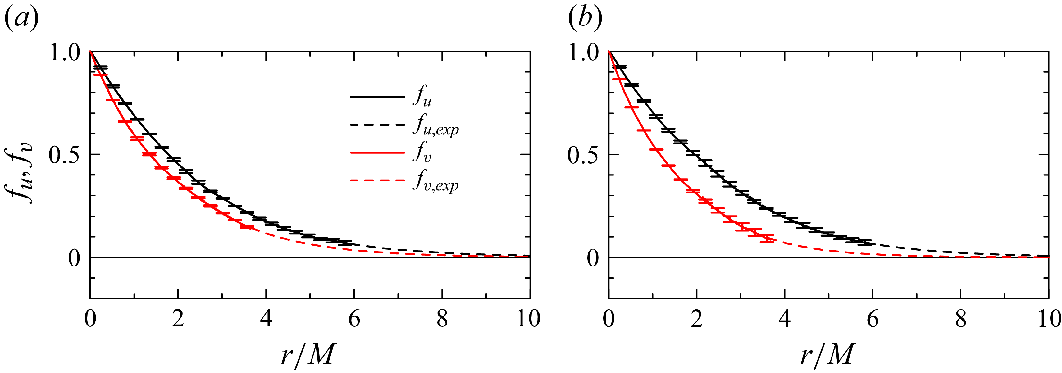
Figure 16 presents
 $f_u$
and
 $f_v$
for cases 1 and 4, representing
 $D_N=930$
and
 $725$
mm. Both
 $f_u$
and
 $f_v$
decrease from unity as
 $r$
increases, indicating decorrelation of velocity fluctuations between two spatially separated points. The measurable range of
 $r$
is limited by the PIV FOV, and although
 $f_u$
and
 $f_v$
are expected to decay to zero, this decay cannot be fully captured. It is known that the tails of autocorrelation functions at large
 $r$
are well approximated by an exponential form
 $a_{\!f}\exp (-b_{\!f}r)$
(Morikawa et al. Reference Morikawa, Urano, Sanada and Saito2008; Bewley, Chang & Bodenschatz Reference Bewley, Chang and Bodenschatz2012; Griffin et al. Reference Griffin, Wei, Bodenschatz and Bewley2019; Mori et al. Reference Mori, Watanabe and Nagata2024). For the measured
 $r$
range where
 $f_u$
and
 $f_v$
fall below 0.3, a least-squares method is used to determine
 $a_{\!f}$
and
 $b_{\!f}$
. The resulting fits,
 $f_{u,{\textit{exp}}}$
and
 $f_{v,{\textit{exp}}}$
, are also shown in figure 16, confirming that the exponential function accurately approximates the measured autocorrelation of both
 $u$
and
 $v$
.
Longitudinal autocorrelation functions of
 $u$
and
 $v$
, denoted by
 $f_u$
and
 $f_v$
, respectively, for (
 $a$
) case 1 and (
 $b$
) case 4. Dashed lines indicate exponential fits that approximate the correlations at large separation distances.

The integral scales are computed by integrating the autocorrelation functions with respect to
 $r$
, defined as
 $L_u=\int f_u(r)\,\textrm{d}r$
and
 $L_v=\int f_v(r)\,\textrm{d}r$
. The integration is performed from
 $r=0$
to the position where the correlation function becomes zero. Since the PIV measurements do not always capture correlations at large
 $r$
, the integral scales are estimated with the aid of the exponential approximations
 $f_{u,{\textit{exp}}}$
and
 $f_{v,{\textit{exp}}}$
, following previous studies (Morikawa et al. Reference Morikawa, Urano, Sanada and Saito2008; Bewley et al. Reference Bewley, Chang and Bodenschatz2012; Griffin et al. Reference Griffin, Wei, Bodenschatz and Bewley2019; Mori et al. Reference Mori, Watanabe and Nagata2024):
 \begin{align} L_{u} = \int _{0}^{r_{1}} f_{u}(r)\,\textrm{d}r + \int _{r_{1}}^{r_{2}} f_{u,{\textit{exp}}}(r)\,\textrm{d}r, \end{align}
where
 $r_1$
is defined by the condition
 $f_u(r_1)=0.3$
and
 $r_{2}$
is the position at which
 $f_{u,{\textit{exp}}}(r)$
reaches
 $1 \times 10^{-5}$
. The integral scale in the
 $y$
direction,
 $L_v$
, is computed in the same manner using
 $f_v$
and
 $f_{v,{\textit{exp}}}$
as in (3.4). Table 1 lists
 $L_u$
,
 $L_v$
and their ratio
 $L_u/L_v$
for each case. Nearly HIT generated by the single jet array yields
 $L_u/L_v\approx 1.03$
(Mori et al. Reference Mori, Watanabe and Nagata2024). In contrast, turbulence subject to axisymmetric expansion in the present experiments exhibits larger values of
 $L_u/L_v$
, indicating increased anisotropy. For the case of the single jet array, both
 $L_u$
and
 $L_v$
are about 0.022 m in the measurement region, comparable to that of the present set-up. Relative to this reference,
 $L_u$
increases and
 $L_v$
tends to decrease in the current experiments, with the deviations from the reference being more pronounced for
 $L_u$
than for
 $L_v$
. Although the case of the single jet array does not provide exact turbulence statistics prior to the onset of mean strain in the OMJA experiments, it is noteworthy that the greater changes observed in
 $L_u$
are consistent with DNS results at low Reynolds numbers of Lee (Reference Lee1989), where
 $L_u$
departs more strongly from the isotropic state than
 $L_v$
under axisymmetric expansion. The increase in
 $L_u$
and the decrease in
 $L_v$
under axisymmetric expansion are also predicted by RDT, which attributes these trends to anisotropic redistribution of energy in three-dimensional wavenumber space and the consequent changes in the one-dimensional spectra (Lee Reference Lee1989).
The scale dependence of velocity fluctuations is examined using longitudinal energy spectra. The Fourier transform of
 $u$
in the
 $x$
direction is denoted by
 $\hat {u}(k_x,y)$
, where
 $k_x$
is the streamwise wavenumber. With
 $\hat {u}^{*}$
representing the complex conjugate of
 $\hat {u}$
, the energy spectrum of
 $u$
is defined as
 $E_u(k_x,y) = \textrm{Re}[\langle \hat {u}\hat {u}^{*}\rangle ]$
, where
 $\textrm{Re}$
denotes the real part. As with the autocorrelation functions, a spatial average in the
 $y$
direction is applied to obtain
 $E_u(k_x)$
. Similarly, the energy spectrum of
 $v$
, denoted by
 $E_v(k_y)$
, is computed from the Fourier transform of
 $v$
in the
 $y$
direction, where
 $k_y$
is the vertical wavenumber.
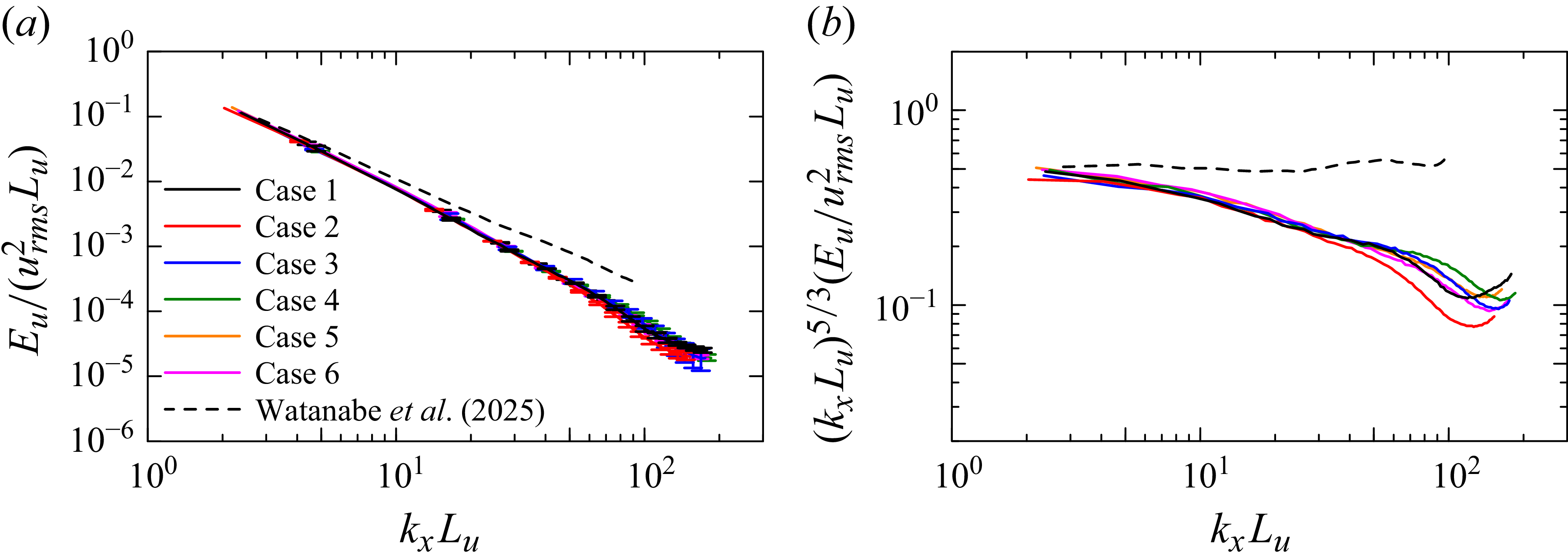
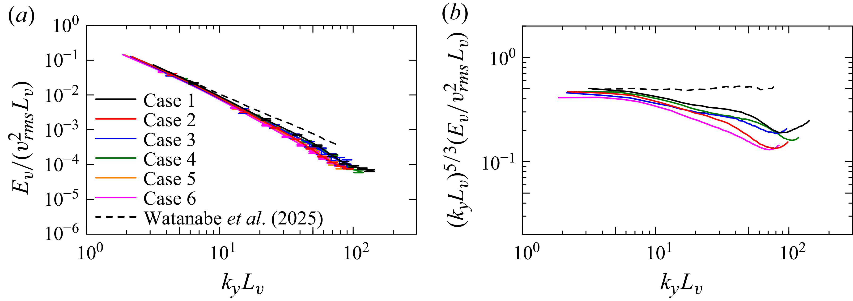
Figures 17(
 $a$
) and 18(
 $a$
) show
 $E_u$
and
 $E_v$
, respectively, together with reference results for nearly HIT generated by the single jet array (Watanabe et al. Reference Watanabe, Inagaki, Mori, Ishizawa and Nagata2025). The accessible wavenumber range is determined by the spatial resolution and the size of the measurement region. As discussed below, the measured range lies within the inertial subrange. In high-Reynolds-number turbulence, Kolmogorov scaling is observed in this subrange, with
 $E_u \sim k_x^{-5/3}$
and
 $E_v \sim k_y^{-5/3}$
. This scaling is more clearly seen in the compensated spectra,
 $k_x^{5/3}E_u$
and
 $k_y^{5/3}E_v$
, shown in figures 17(
 $b$
) and 18(
 $b$
). The
 $-5/3$
law appears as a plateau in the compensated spectra and is evident in the single-jet-array results. In contrast, the present experiments show that
 $k_x^{5/3}E_u$
and
 $k_y^{5/3}E_v$
decrease with increasing
 $k_x$
and
 $k_y$
, indicating a faster decay than predicted by the
 $-5/3$
law.
(
 $a$
) Longitudinal energy spectra of
 $x$
-directional velocity fluctuations,
 $E_u(k_x)$
, where
 $k_x$
is the
 $x$
-directional wavenumber. (
 $b$
) Compensated spectra
 $k_x^{5/3}E_u$
. Results for nearly HIT generated by the single jet array, evaluated 605 mm downstream of the nozzles, are shown for comparison (Watanabe et al. Reference Watanabe, Inagaki, Mori, Ishizawa and Nagata2025).

(
 $a$
) Longitudinal energy spectra of
 $y$
-directional velocity fluctuations,
 $E_v(k_y)$
, where
 $k_y$
is the
 $y$
-directional wavenumber. (
 $b$
) Compensated spectra
 $k_y^{5/3}E_v$
. Results for nearly HIT generated by the single jet array, evaluated 605 mm downstream of the nozzles, are shown for comparison (Watanabe et al. Reference Watanabe, Inagaki, Mori, Ishizawa and Nagata2025).

Previous studies of HIT subject to axisymmetric contraction, based on DNS and wind tunnel experiments, reported deviations in the opposite direction, where the spectra decay more slowly than the
 $-5/3$
law (Ayyalasomayajula & Warhaft Reference Ayyalasomayajula and Warhaft2006; Clay & Yeung Reference Clay and Yeung2016). In contrast, the present results demonstrate that axisymmetric expansion leads to faster decay. This deviation from the
 $-5/3$
law under axisymmetric expansion could not be assessed in previous DNS because the Reynolds numbers were too low (Lee Reference Lee1989). The mean velocity gradient tensors for axisymmetric contraction and expansion can be expressed in the same form with opposite signs using a single strain-rate parameter
 $S\gt 0$
, as shown in (1.2) and (1.3). These forms indicate that contraction and expansion exert opposite effects on turbulence. In this context, the faster decay in
 $E_u$
and
 $E_v$
observed here under axisymmetric expansion aligns with earlier findings for axisymmetric contraction.
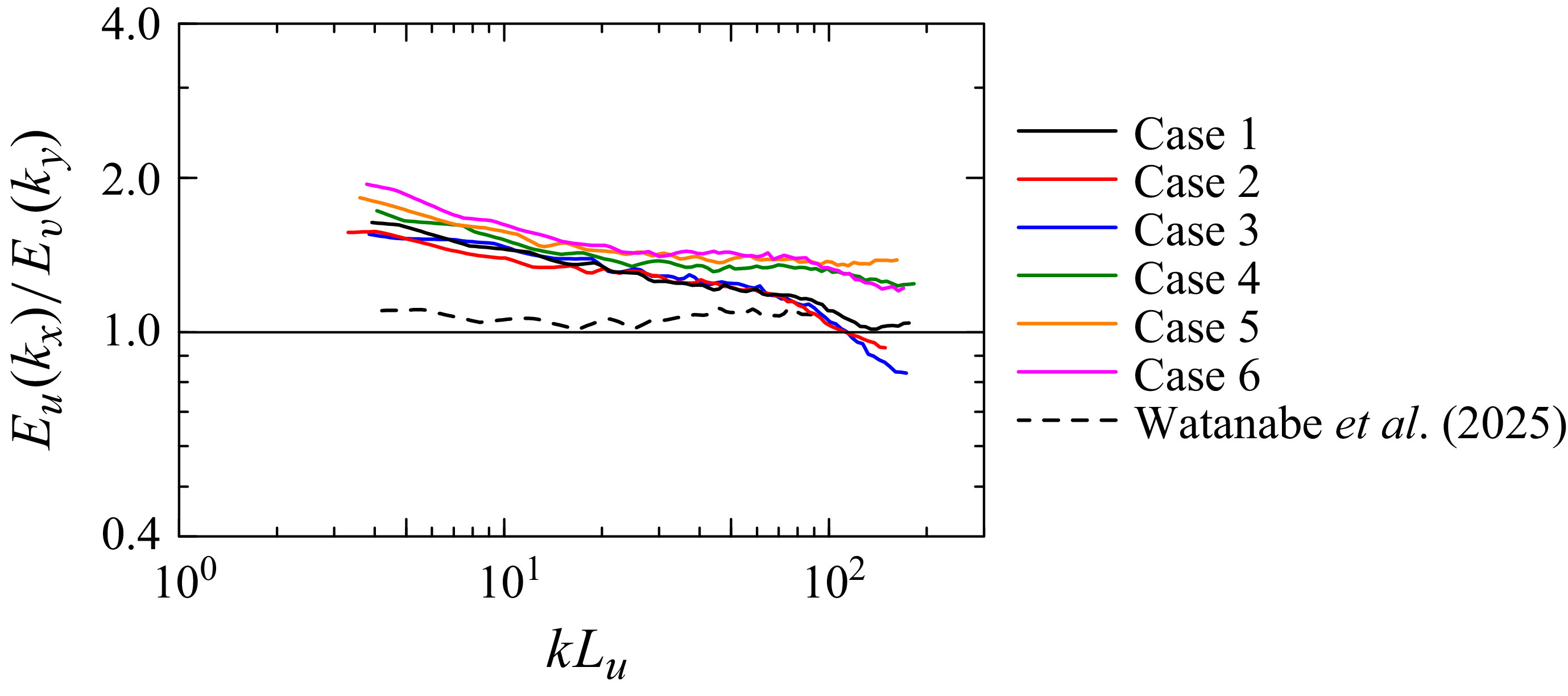
Figure 19 shows
 $E_u/E_v$
calculated at identical wavenumber values
 $k = k_x = k_y$
, providing a measure of anisotropy at each scale. The result for the single jet array is also included for comparison (Watanabe et al. Reference Watanabe, Inagaki, Mori, Ishizawa and Nagata2025). For the single jet array,
 $E_u/E_v$
remains close to 1.05 across all wavenumbers, indicating approximate isotropy at all scales. In contrast, the present results show
 $E_u/E_v \gt 1.2$
over most wavenumbers. As
 $E_u/E_v$
decreases with increasing wavenumber, the velocity fluctuations are more anisotropic at larger scales, where the influence of mean strain is more pronounced. Generally, smaller-scale turbulent motions have shorter characteristic time scales. Since the time scale of the mean strain is determined by the mean velocity gradients, it acts relatively slowly on such small-scale motions. Consequently, the direct effect of mean strain is weaker at small scales, which explains why the greatest deviation from
 $E_u/E_v \approx 1$
appears at larger scales.
Ratios of energy spectra of
 $u$
and
 $v$
,
 $E_u/E_v$
. Results for nearly HIT generated by the single jet array, evaluated 605 mm downstream of the nozzles, are shown for comparison (Watanabe et al. Reference Watanabe, Inagaki, Mori, Ishizawa and Nagata2025).

The energy spectra describe the scale-by-scale distribution of turbulent kinetic energy in wavenumber space. A real-space equivalent is the second-order structure function, defined using the velocity difference between two points (Davidson Reference Davidson2015). The longitudinal structure function of
 $u$
is given by
 $\langle (\Delta u)^2 \rangle$
, where
 $\Delta u = u'(x + r/2, y) - u'(x - r/2, y)$
. In the inertial subrange, the scaling
 $\langle (\Delta u)^2 \rangle \sim r^{2/3}$
corresponds to the spectral scaling
 $E_u \sim k_x^{-5/3}$
. More generally, Kolmogorov’s second similarity hypothesis predicts that the
 $n$
th-order longitudinal structure function scales as
 $r^{n/3}$
(Kolmogorov Reference Kolmogorov1991a
,
Reference Kolmogorovb
; Tsinober Reference Tsinober2009; Davidson Reference Davidson2015). Previous studies have shown that the scaling exponents deviate from
 $n/3$
as
 $n$
increases, a phenomenon attributed to small-scale intermittency. The deviation becomes pronounced for
 $n \geqslant 5$
(Arneodo et al. Reference Arneodo1996; Saw et al. Reference Saw, Debue, Kuzzay, Daviaud and Dubrulle2018; Iyer, Sreenivasan & Yeung Reference Iyer, Sreenivasan and Yeung2020). The present results for the energy spectra deviating from the
 $k_x^{-5/3}$
scaling imply that the structure functions deviate from the
 $n/3$
scaling even for small
 $n$
, with the departures arising from mechanisms other than small-scale intermittency.
We evaluate the
 $n$
th-order longitudinal structure function of
 $u'$
as
 $\langle |\Delta u|^n \rangle = \langle |u'(x + r/2, y) - u'(x - r/2, y)|^n \rangle$
at
 $x = 0$
, using ensemble averages combined with spatial averages in the
 $y$
direction. Similarly, the longitudinal structure function of
 $v'$
is computed at
 $y=0$
as
 $\langle |\Delta v|^n \rangle = \langle |v'(x, y + r/2) - v'(x, y - r/2)|^n \rangle$
, using ensemble averaging together with spatial averaging in the
 $x$
direction. Figure 20(
 $a$
) shows the third- and fifth-order structure functions together with the power laws
 $r^{n/3}$
. We set the maximum separation to
 $r/M=0.75$
so that
 $r\leqslant L_u/3$
. Below this bound the structure functions exhibit clear power laws and the
 $-5/3$
spectral slope is observed at the corresponding wavenumbers for the single-jet-array case (Watanabe et al. Reference Watanabe, Mori, Ishizawa and Nagata2024). In contrast, for turbulence subject to axisymmetric expansion, both the third- and fifth-order structure functions follow power-law behaviour but with exponents that deviate substantially from
 $n/3$
.
(
 $a$
) Third- and fifth-order structure functions for case 4. Solid lines indicate the power laws predicted by Kolmogorov’s second similarity hypothesis. (
 $b$
) Power-law exponents
 $p$
for the
 $n$
th-order structure functions. Present results are compared with DNS of isotropic turbulence (Iyer et al. Reference Iyer, Sreenivasan and Yeung2020) and experimental data for various turbulent flows, including jets, wakes, mixing layers, duct flows and grid turbulence (Arneodo et al. Reference Arneodo1996), as well as nearly HIT generated by the same single jet array used in this study (Watanabe et al. Reference Watanabe, Mori, Ishizawa and Nagata2024).

Figure 20(
 $b$
) shows the power-law exponents
 $p$
of the
 $n$
th-order longitudinal structure functions of
 $u$
and
 $v$
, obtained by least-squares fitting. The present results are compared with reference data from DNS of isotropic turbulence (Iyer et al. Reference Iyer, Sreenivasan and Yeung2020) and from experiments of various flows (Arneodo et al. Reference Arneodo1996). Results for nearly HIT generated by the single jet array at
 $\textit{Re}_\lambda \approx 600$
(Watanabe et al. Reference Watanabe, Mori, Ishizawa and Nagata2024), obtained with the same PIV set-up, are also shown. In Watanabe et al. (Reference Watanabe, Mori, Ishizawa and Nagata2024), the available range of
 $r$
, set by the spatial resolution and FOV of the PIV, is similar to that of the present measurements. Although the fitting range spans less than one decade, the exponents for the single jet array agree well with DNS and experimental data, confirming that the limited
 $r$
range does not compromise exponent evaluation. For these reference cases, the exponents follow
 $p=n/3$
predicted by Kolmogorov’s second similarity hypothesis for
 $n \leqslant 4$
, but become smaller than
 $n/3$
as
 $n$
increases, reflecting small-scale intermittency. In contrast, the present results for turbulence subject to axisymmetric expansion yield exponents larger than
 $n/3$
, in clear departure from other turbulent flows. The departure is similar for
 $u$
and
 $v$
. Since the single-jet-array results reproduce established turbulence data, the observed deviation is most likely due to mean strain effects. The energy spectra exhibit a faster decay than
 $k_x^{-5/3}$
, consistent with an exponent for
 $n=2$
exceeding
 $2/3$
; indeed,
 $p(n=2)=1.1$
for
 $\langle |\Delta u|^n \rangle$
and 0.98 for
 $\langle |\Delta v|^n \rangle$
is obtained. Previous comparisons across grid turbulence, jets, mixing layers and cylinder wakes have shown that mean shear exerts little influence on the scaling of structure functions (Arneodo et al. Reference Arneodo1996). Consistently, numerous experiments and numerical simulations have reported the persistence of the
 $-5/3$
energy spectral law in canonical turbulent shear flows (Uberoi & Freymuth Reference Uberoi and Freymuth1970; Fiscaletti et al. Reference Fiscaletti, Elsinga, Attili, Bisetti and Buxton2016; Sadeghi, Oberlack & Gauding Reference Sadeghi, Oberlack and Gauding2018; Takamure et al. Reference Takamure, Sakai, Ito, Iwano and Hayase2019; Watanabe, Zhang & Nagata Reference Watanabe, Zhang and Nagata2019). Taken together with reports of non-
 $-5/3$
spectra for turbulence under axisymmetric contraction (Ayyalasomayajula & Warhaft Reference Ayyalasomayajula and Warhaft2006), the present findings for axisymmetric expansion suggest that mean axisymmetric strain exerts a stronger influence on structure–function scaling than mean shear.
The turbulent kinetic energy distribution across scales can be examined using second-order structure functions, which estimate the kinetic energy contained in scales below a given separation distance (Davidson Reference Davidson2015). The transport equation for the second-order structure function is often utilised to assess the scale-dependent energy budget (Deissler Reference Deissler1992; Valente & Vassilicos Reference Valente and Vassilicos2015; Wang et al. Reference Wang, Yurikusa, Iwano, Sakai, Ito, Zhou and Hattori2023). This scale-by-scale energy-transport equation, originating from the Kármán–Howarth equation, contains two inviscid terms that describe interscale energy transfers: a nonlinear transfer due to turbulent fluctuations and a linear transfer due to mean velocity gradients. For the longitudinal structure functions of
 $u$
and
 $v$
, which are related to the longitudinal energy spectra in figures 17 and 18, the relevant nonlinear transfer terms measured on the
 $x$
–
 $y$
plane at
 $z=0$
are
 \begin{align} \varPi _{u'}(x,y,r)&=-\frac {\partial \left\langle [u'(x^+,y) - u'(x^-,y)]^3\right\rangle }{\partial r}, \end{align}
 \begin{align} \varPi _{v'}(x,y,r)&=-\frac {\partial \left\langle [v'(x,y^+) - v'(x,y^-)]^3\right\rangle }{\partial r}, \end{align}
with
 $x^+=x+r/2$
,
 $x^-=x-r/2$
,
 $y^+=y+r/2$
and
 $y^-=y-r/2$
, as derived in Valente & Vassilicos (Reference Valente and Vassilicos2015). The corresponding linear transfer terms are
 \begin{align} \varPi _{\langle u\rangle }(x,y,r)&= -\frac {\partial [\langle u\rangle (x^+,y) - \langle u\rangle (x^-,y)] \left\langle [u'(x^+,y) - u'(x^-,y)]^2\right\rangle }{\partial r}, \end{align}
 \begin{align} \varPi _{\langle v\rangle }(x,y,r)&= -\frac {\partial [\langle v\rangle (x,y^+) - \langle v\rangle (x,y^-)] \left\langle [v'(x,y^+) - v'(x,y^-)]^2\right\rangle }{\partial r}. \end{align}
Figure 21 shows these terms at
 $(x,y)=(0,0)$
normalised by
 $u_{\textit{rms}}^{3}/L_u$
or
 $v_{\textit{rms}}^{3}/L_v$
. A second-order central difference is used for
 $\partial /\partial r$
. Because small errors in the structure functions can be amplified by differentiation, we focus on the overall trends rather than precise quantification. The maximum separation for evaluation is
 $r=1.8M$
, close to the integral scales. Positive and negative values indicate transfers to smaller and larger scales (forward and backward transfers), respectively. Thus,
 $\varPi _{\langle u\rangle }\gt 0$
and
 $\varPi _{\langle v\rangle }\lt 0$
show that the mean velocity gradients associated with axisymmetric expansion have opposite effects: compression in the
 $x$
direction gives
 $\langle u\rangle (x^+,y)-\langle u\rangle (x^-,y)\lt 0$
and hence a forward transfer with
 $\varPi _{\langle u\rangle }\gt 0$
, whereas expansion in the
 $y$
direction yields
 $\langle v\rangle (x,y^+)-\langle v\rangle (x,y^-)\gt 0$
and thus a backward transfer with
 $\varPi _{\langle v\rangle }\lt 0$
. At large scales, the linear transfer terms exceed the nonlinear ones. Even at
 $r/L_u\approx 10^{-1}$
and
 $r/L_v\approx 10^{-1}$
they are of comparable magnitude. Thus, the mean velocity gradients of axisymmetric expansion alter the energy transfer across scales. The nonlinear terms also differ substantially between components. The
 $x$
-component
 $\varPi _{u'}$
is positive, indicating forward transfer that diminishes as
 $r$
approaches the integral scale, consistent with other turbulent flows (Valente & Vassilicos Reference Valente and Vassilicos2015). In general, the nonlinear term scales as
 $u_{\textit{rms}}^{3}/L_u$
(or
 $v_{\textit{rms}}^{3}/L_v$
), and the normalised quantity
 $\varPi _{u'}/(u_{\textit{rms}}^{3}/L_u)$
is close to 1. By contrast, the
 $y$
-component
 $\varPi _{v'}$
becomes negative at large scales, indicating that axisymmetric expansion modifies the nonlinear transfer. Deviations from the
 $-5/3$
law are observed in the longitudinal energy spectra of both
 $u$
and
 $v$
. Since axisymmetric expansion affects the interscale transfers of these components differently, the spectral changes are unlikely to be explained solely by the interscale transfers.
Linear and nonlinear longitudinal interscale energy transfers defined by (3.5)–(3.8). (
 $a$
) Energy transfer of the
 $x$
-directional velocity across scales in the
 $x$
direction; (
 $b$
) energy transfer of the
 $y$
-directional velocity across scales in the
 $y$
direction. The separation distance and energy-transfer terms are normalised by the integral scales and r.m.s. velocity fluctuations.

3.4. Summary of turbulence statistics
Table 1 summarises velocity statistics obtained for all experimental conditions with different test-section geometries. The dissipation scaling is used to provide an order-of-magnitude estimate of the turbulent kinetic energy dissipation rate per unit mass,
 $\varepsilon = A\mathcal{U}^3/\mathcal{L}$
, where
 $\mathcal{U}$
and
 $\mathcal{L}$
denote the large-scale velocity and length scales. The present analysis relies on this dissipation scaling because the PIV does not resolve the smallest turbulent scales. The non-dimensional constant
 $A$
varies among flows and may depend on position in the present set-up, but
 $A=O(10^0)$
holds in most cases, including nearly HIT generated by the single jet array (Mori et al. Reference Mori, Watanabe and Nagata2024). We therefore take
 $A=1$
for the present estimates. This approximation is used only to evaluate the orders of the Taylor microscale
 $\lambda$
, the Kolmogorov scale
 $\eta$
and the turbulent Reynolds number
 $\textit{Re}_\lambda$
; accurate values of these quantities would require direct measurements of
 $\varepsilon$
. The velocity and length scales are defined as
 $\mathcal{U}=\sqrt {2k_T/3}$
and
 $\mathcal{L}=(L_u+L_v+L_w)/3$
, where the turbulent kinetic energy is
 $k_T=(\langle u^{\prime 2}\rangle +\langle v^{\prime 2}\rangle +\langle w^{\prime 2}\rangle )/2$
and
 $L_w$
is the integral scale in the
 $z$
direction. With statistical equivalence in the
 $y$
and
 $z$
directions, we assume
 $\langle w^{\prime 2}\rangle =\langle v^{\prime 2}\rangle$
and
 $L_w=L_v$
. The Taylor microscale and Kolmogorov scale are given by
 $\lambda =\sqrt {10(\mu /\rho )k_T/\varepsilon }$
and
 $\eta =(\mu /\rho )^{3/4}\varepsilon ^{-1/4}$
, respectively. The turbulent Reynolds number is
 $\textit{Re}_\lambda =\rho \sqrt {2k_T/3}\,\lambda /\mu$
. The resulting values of
 $k_T$
,
 $\varepsilon$
,
 $\lambda$
,
 $\eta$
and
 $\textit{Re}_\lambda$
are listed in table 1.
The Kolmogorov scales are
 $\eta /M \approx 1 \times 10^{-3}$
for cases 1–3 and
 $0.7\times 10^{-3}$
for cases 4–6. The larger
 $\eta$
in the former cases reflects the longer inner ducts with larger
 $D_N$
, as turbulence decay increases
 $\eta$
. Turbulence decay also enlarges the Taylor microscale, giving
 $\lambda$
values greater in cases 1–3 than in cases 4–6. Consistently,
 $\textit{Re}_\lambda$
is about 600 for cases 1–3 and 700 for cases 4–6. These values are sufficiently large to allow observation of the inertial subrange with the
 $-5/3$
law, as this scaling and its structure–function equivalent have been successfully observed in turbulence generated by the single jet array at comparable
 $\textit{Re}_\lambda$
(Mori et al. Reference Mori, Watanabe and Nagata2024; Watanabe et al. Reference Watanabe, Mori, Ishizawa and Nagata2024). The observed deviation from the
 $-5/3$
law is therefore unlikely to originate from low-Reynolds-number effects. Consistently, turbulence subject to axisymmetric contraction at similar
 $\textit{Re}_\lambda$
also departs from the
 $-5/3$
scaling, as discussed above (Ayyalasomayajula & Warhaft Reference Ayyalasomayajula and Warhaft2006).
An important parameter describing the influence of mean strain on turbulence is the ratio of the strain time scale to the turbulence time scale. From (1.3), the strain rate
 $S$
is evaluated from the experimental data as
 $S = (|\mathsf{A}_{\textit{xx}}| + 2\mathsf{A}_{\textit{yy}} + 2\mathsf{A}_{zz})/3,$
using the continuity relation
 $\mathsf{A}_{zz} = -\mathsf{A}_{\textit{xx}} - \mathsf{A}_{\textit{yy}}$
. The characteristic time scale of large-scale motion is defined as
 $T_L = {\mathcal L}/{\mathcal U}$
. The normalised strain rate is expressed as
 $ST_L$
, representing the ratio of
 $T_L$
to the strain time scale
 $1/S$
. Table 1 lists
 $ST_L$
values for all cases. In all experiments,
 $ST_L$
is close to unity, indicating that the mean strain acts on a time scale comparable to that of large-scale turbulent motions. Comparisons among cases suggest that the distance between the two opposing jet arrays,
 $D_N$
, has a stronger influence on
 $ST_L$
, through turbulence decay effects on
 $T_L$
, than the gap length between the inner-duct exits,
 $D_E$
, which affects
 $S$
. Systematic experiments varying
 $D_N$
would therefore be valuable for further investigations of turbulence under axisymmetric strain.
Turbulence generated by the OMJA facility exhibits
 $ST_L \approx 1$
while the necessary condition for the RDT assumption to be valid is
 $ST_L \gg 1$
. Nonetheless, several findings are qualitatively consistent with RDT. Detailed comparisons with RDT require knowledge of the total strain (distortion) experienced along mean flow trajectories. When the turbulence intensity is small, this can be inferred from spatial variations of the mean velocity using Taylor’s frozen-turbulence hypothesis, as in wind tunnel studies of axisymmetric contraction. In the present set-up, however, the turbulence intensity is very high near the stagnation region, owing to the small mean velocity there and to the jet-interaction turbulence, so this approach is not suitable.
Rapid distortion theory for axisymmetric turbulence has been presented in previous studies (Batchelor Reference Batchelor1946; Sreenivasan & Narasimha Reference Sreenivasan and Narasimha1978; Hunt & Carruthers Reference Hunt and Carruthers1990). Based on these frameworks, temporal evolutions of
 $u_{\textit{rms}}/v_{\textit{rms}}$
and
 $L_u/L_v$
under axisymmetric expansion have been derived (Pope Reference Pope1985; Lee Reference Lee1989). For initially HIT, RDT predicts that axisymmetric expansion induces anisotropy, increasing both
 $u_{\textit{rms}}/v_{\textit{rms}}$
and
 $L_u/L_v$
above unity. The present measurements likewise show
 $u_{\textit{rms}}/v_{\textit{rms}}\gt 1$
and
 $L_u/L_v\gt 1$
. However, RDT predicts an upper bound
 $u_{\textit{rms}}/v_{\textit{rms}}=\sqrt {2}$
, whereas our results exceed this limit (Pope Reference Pope2000). Consistently, other experiments and DNS on turbulence with axisymmetric expansion at low Reynolds numbers report greater anisotropy than RDT when the strain time scale is comparable to turbulence time scales (Liu et al. Reference Liu, Katz and Meneveau1999; Choi & Lumley Reference Choi and Lumley2001). In addition, RDT predicts that axisymmetric strain does not modify the
 $-5/3$
slope of the energy spectra at high Reynolds numbers, as shown in Appendix A. This contrasts with the present results in figures 17 and 18 and with previous findings for axisymmetric contraction (Ayyalasomayajula & Warhaft Reference Ayyalasomayajula and Warhaft2006).
4. Conclusion
A novel turbulence facility with opposing multiple-jet arrays has been developed to investigate turbulence subject to axisymmetric expansion at large Reynolds numbers. The facility employs two opposed jet generators, each producing
 $6\times 6$
supersonic jets, and their interaction forms nearly HIT. The collision of the opposing turbulent flows creates a stagnation region in the mean field, inducing axisymmetric expansion. Velocity measurements using two-component PIV have revealed both the mean strain and turbulence characteristics. The axisymmetric expansion, with mean velocity gradients satisfying
 $\mathsf{A}_{\textit{xx}}:\mathsf{A}_{\textit{yy}}:\mathsf{A}_{zz} = -2:1:1$
and
 $\mathsf{A}_{\textit{xx}} \lt 0$
, is uniformly established near the centre of the test section. However, the strain rate, defined as
 $|\mathsf{A}_{\textit{xx}}|$
, varies spatially and becomes larger towards the centre along the symmetry axis.
Turbulence generated by each jet array is nearly homogeneous and isotropic, but becomes anisotropic under axisymmetric expansion. In particular, the ratios
 $u_{\textit{rms}}/v_{\textit{rms}}$
and
 $L_u/L_v$
increase compared with those in nearly HIT generated by the single jet array. The invariant of the normalised anisotropy tensor of the Reynolds stress indicates that the flow becomes increasingly anisotropic towards the centre of the test section, reflecting the cumulative effect of mean strain. This anisotropy is qualitatively consistent with RDT predictions for initially isotropic turbulence subject to mean strain, which also predicts
 $u_{\textit{rms}}/v_{\textit{rms}}\gt 1$
and
 $L_u/L_v\gt 1$
. However, the present experiments do not satisfy RDT assumptions, since the strain time scale is close to that of large-scale turbulent motions, and several deviations from RDT predictions are observed. The measured values of
 $u_{\textit{rms}}/v_{\textit{rms}}$
exceed the upper bound predicted by RDT. Furthermore, the energy spectra decay faster than the
 $-5/3$
law. Consistently, the scaling exponents of velocity structure functions deviate from the prediction based on Kolmogorov’s second similarity hypothesis, even for low-order structure functions. The linear interscale transfer of turbulent kinetic energy due to mean velocity gradients is comparable to the nonlinear contribution at large scales, inducing forward and backward transfers for
 $u$
and
 $v$
, respectively; nevertheless, both components exhibit similar departures from the
 $-5/3$
law, suggesting that the modified interscale transfer is not the primary cause of these departures. Since RDT does not capture these changes in the scaling laws, the results motivate further studies of the influence of mean strain on turbulence, ideally via high-Reynolds-number DNS. Unlike mean shear, which has little effect on the scaling laws (Arneodo et al. Reference Arneodo1996), the present findings demonstrate that axisymmetric mean strain significantly alters turbulence properties that are otherwise considered universal.
The anomalous behaviours of the spectra and structure functions are consistent with reports for turbulence under axisymmetric contraction, where the deviation from the
 $-5/3$
law has been reported (Ayyalasomayajula & Warhaft Reference Ayyalasomayajula and Warhaft2006). The underlying cause of this departure remains unresolved and has received limited attention. Our results show that analogous deviations arise under axisymmetric expansion as well as compression, indicating a common influence of mean axisymmetric strain on inertial-range statistics. Given the central role of inertial-range scaling in turbulence theory and modelling, this deviation merits further investigation.
In the opposed multiple-jet array set-up, different test-section geometries enable experiments with varied strain and turbulence conditions. Extending the inner ducts increases turbulence decay before it reaches the strain region, thereby modifying its properties. Varying the gap between duct ends alters the strain rate, although it is not determined solely by this gap. The present study is limited to narrow ranges of these geometric parameters due to the number of available nozzles, constrained by the air tank volume. Nevertheless, the results demonstrate that the opposed multiple-jet array configuration offers a useful platform for parametric studies of turbulence under axisymmetric expansion, particularly when larger numbers of jets and extended test sections become available.
Acknowledgements
The authors gratefully acknowledge the technical support provided during the setting up of the experimental facility by Mr Sato, Mr Tamaki and Mr Hatano of the Mechanical Engineering Group, Department of Mechanical Engineering and Science, Kyoto University. The authors used an AI-assisted language tool to improve readability for grammatical accuracy, spelling and clarity; all content was verified and approved by the authors, who take full responsibility for the text.
Funding
This work was supported by JSPS KAKENHI grant nos. JP23K22669 and JP25K01155. Z.H. also acknowledges financial support from the Amano Institute of Technology Scholarship.
Declaration of interests
The authors report no conflict of interest.
Data availability statement
The data that support the findings of this study are available from the corresponding author upon reasonable request.
Appendix A. Rapid distortion theory for turbulence subject to axisymmetric expansion
The present experiments demonstrate that axisymmetric expansion modifies the energy spectrum, which no longer follows the
 $-5/3$
law in the inertial subrange. This appendix examines these spectral changes in the framework of RDT and shows that the experimental results are inconsistent with RDT predictions. Similar discrepancies between RDT and measured spectra have also been reported in DNS and experiments of turbulence subject to axisymmetric contraction (Ayyalasomayajula & Warhaft Reference Ayyalasomayajula and Warhaft2006; Clay & Yeung Reference Clay and Yeung2016).
We briefly outline RDT for turbulence subject to axisymmetric strain, following Batchelor (Reference Batchelor1953); further details can be found in the original reference. The deformation of a fluid element
 $\partial x \partial y \partial z$
in initially isotropic turbulence under axisymmetric strain is given by
 \begin{align} \frac {\partial x^*}{\partial x} = c, \quad \frac {\partial y^*}{\partial y} = \frac {\partial z^*}{\partial z} = \frac {1}{\sqrt {c}}, \quad \frac {\partial x_i^*}{\partial x_{\!j}} = 0 \ \textrm{for} \ i \neq j, \end{align}
where
 $\partial x^* \partial y^* \partial z^*$
denotes the post-deformation element and
 $c$
characterises the imposed strain;
 $x$
indicates the direction of the strain axis, while
 $y$
and
 $z$
denote the transverse directions. Axisymmetric contraction and expansion correspond to
 $c \gt 1$
and
 $c \lt 1$
, respectively. An asterisk denotes quantities in the strained state, while unstarred symbols denote those in the initial state.
The general form of the energy spectrum tensor for turbulence under arbitrary irrotational strain was derived by Batchelor (Reference Batchelor1953). Based on the spectrum tensor for axisymmetric strain given therein, the longitudinal energy spectrum in the
 $x$
direction after deformation is
 \begin{align} E_{u}^*(k_x^*) = \iint \frac {E(k)}{2\pi {k^*}^4}(k_y^2+k_z^2)\, \textrm{d}k_y^* \,\textrm{d}k_z^*, \end{align}
where the strained wavenumbers
 $k_i^*$
are related to the original wavenumbers
 $k_i$
by
 \begin{align} k_x^* = \frac {k_x}{c}, \quad k_y^* = \sqrt {c}\,k_y, \quad k_z^* = \sqrt {c}\,k_z, \end{align}
and
 $E(k)$
denotes the three-dimensional energy spectrum of the initial isotropic state with wavenumber
 $k$
.
The strain effects can be evaluated with RDT by numerically integrating (A2) using a prescribed form of
 $E(k)$
. Here we adopt the model spectrum of Pope (Reference Pope2000):
 \begin{align} E(k) &= C \varepsilon ^{2/3} k^{-5/3} f_L(kL_k) f_\eta (k\eta ), \end{align}
 \begin{align} f_L(kL_k) &= \left ( \frac {kL_k}{\sqrt {(kL_k)^2 + c_L}} \right )^{5/3 + p_0}, \end{align}
 \begin{align} f_\eta (k\eta ) &= \exp \left \{ -\beta \left ( \left [ (k\eta )^4 + c_{\eta }^4 \right ]^{1/4} - c_{\eta } \right ) \right \}\!, \end{align}
where
 $C = 1.5$
is the Kolmogorov constant,
 $\varepsilon$
the energy dissipation rate,
 $L_k$
the integral length scale and
 $\eta$
the Kolmogorov length scale. The integral scale is defined as
 $L_k = k_T^{3/2}/\varepsilon$
with the turbulent kinetic energy
 $k_T$
. This definition is different from the integral scales in § 3.3, where the integrations of autocorrelation functions yield the integral scales. The Taylor microscale is
 $\lambda = \sqrt {10k_T\nu /\varepsilon }$
, with
 $\nu$
the kinematic viscosity, and the turbulent Reynolds number is
 $\textit{Re}_\lambda = \sqrt {2k_T/3}\,\lambda /\nu$
. We consider an initial isotropic turbulence with r.m.s. velocity
 $\sqrt {2k_T/3} = 1$
and integral scale
 $L = 1$
in arbitrary units. Specifying
 $\textit{Re}_\lambda$
then fixes
 $\nu$
and
 $\varepsilon$
, which are used to evaluate
 $E(k)$
.
The post-deformation spectra are computed from (A2) for
 $\textit{Re}_\lambda = 600$
with
 $c = 0.25$
. We have confirmed that varying
 $c$
does not affect the shape of the energy spectra. Figure 22(
 $a$
) compares the longitudinal energy spectrum of the
 $x$
-directional velocity before and after deformation. The post-deformation spectrum is shifted upward relative to the initial isotropic state, indicating enhanced velocity fluctuations, consistent with the present experimental observations. In both pre- and post-deformation spectra, the inertial-range scaling
 $E_u \sim k_x^{-5/3}$
is clearly observed. This is further demonstrated in the compensated spectra
 $k_x^{5/3}E_u$
in figure 22(
 $b$
), where the plateau region is nearly identical for both cases. Although not shown, axisymmetric contraction with
 $c \gt 1$
exhibits the same trend, with negligible deformation effects on the
 $k_x^{-5/3}$
scaling. These RDT predictions contradict the present results for axisymmetric expansion and previous findings for axisymmetric contraction (Ayyalasomayajula & Warhaft Reference Ayyalasomayajula and Warhaft2006; Clay & Yeung Reference Clay and Yeung2016), suggesting that nonlinear effects play a significant role in both strain types.
Longitudinal energy spectra of
 $x$
-directional velocity fluctuations,
 $E_u(k_x)$
, before and after deformation due to axisymmetric expansion. The post-deformation spectrum is computed using RDT with (A2).