3.1. Initialization

As mentioned in § 2, we initialize $\eta$ and $\varPhi _s$ from the JONSWAP spectrum $J(\omega , \theta ) = S(\omega ) D(\theta )$ with $S(\omega )$ and $D(\theta )$ given by (2.2) and (2.4), respectively. The adopted numerical method for the solution of (2.1) approximates $\eta$ and $\varPhi _s$ in terms of truncated Fourier series, i.e.

(3.1a)\begin{gather} \eta(x,y,t) = \sum_{n_x ={-}N_x}^{N_x-1} \sum_{n_y ={-}N_y}^{N_y-1} \hat{\eta}_{n_x, n_y}(t) \exp ( \text{i} \boldsymbol{k}_{n_x, n_y} \cdot \boldsymbol{r} ), \end{gather}

(3.1b)\begin{gather}\varPhi_s(x,y,t) = \sum_{n_x ={-}N_x}^{N_x-1} \sum_{n_y ={-}N_y}^{N_y-1} \hat{\varPhi}_{n_x, n_y}(t) \exp ( \text{i} \boldsymbol{k}_{n_x, n_y} \cdot \boldsymbol{r} ), \end{gather}

and, therefore, the initialization procedure consists of computing the expansion coefficients $\hat {\eta }_{n_x, n_y}$ and $\hat {\varPhi }_{n_x, n_y}$ corresponding to $J(\omega ,\theta )$ with random phases. Here $\boldsymbol {r} = (x,y)$ denotes the horizontal position and $\boldsymbol {k}_{n_x, n_y} = (2{\rm \pi} n_x/L_x, 2{\rm \pi} n_y/L_y)$ is the $(n_x, n_y)$th wavenumber vector. In order to compute the initial coefficients, we follow Tanaka (Reference Tanaka2001) and start by computing the number

(3.2)\begin{equation} b_{n_x, n_y} = \left( \frac{2{\rm \pi}^2 g^3}{ \omega_{n_x, n_y}^4 L_x L_y} J(\omega_{n_x, n_y}, \theta_{n_x, n_y}) \right)^{1/2} \exp({\text{i} \phi_{n_x, n_y}}), \end{equation}

where $\omega _{n_x, n_y} = ( g | \boldsymbol {k}_{n_x, n_y} | )^{1/2}$ is the $(n_x, n_y)$th frequency, $\phi _{n_x, n_y}$ is a random number drawn from a uniform distribution over the interval $[0, 2{\rm \pi} ]$ and $\theta _{n_x, n_y}$ is the angle between $\boldsymbol {k}_{n_x, n_y}$ and the $x$-axis measured positively in the counter clockwise direction. From $b_{n_x, n_y}$ we then compute the initial coefficients as

(3.3a)\begin{gather} \hat{\eta}_{n_x, n_y} = \left( \frac{|\boldsymbol{k}_{n_x, n_y}|}{ 2 \omega_{n_x, n_y}} \right)^{1/2} ( b_{n_x, n_y} + b_{{-}n_x, -n_y}^{{\ast}} ), \end{gather}

(3.3b)\begin{gather}\hat{\varPhi}_{n_x, n_y} ={-} \text{i} \left( \frac{\omega_{n_x, n_y}}{2 |\boldsymbol{k}_{n_x, n_y}|} \right)^{1/2} ( b_{n_x, n_y} - b_{{-}n_x, -n_y}^{{\ast}} ), \end{gather}

where the symbol $^\ast$ denotes complex conjugation. We note that this initialization procedure gives a wave field which is consistent with the governing equations only when these are linearized around the rest state. For that reason, the initial surface elevation should in all simulations ideally be normally distributed. With the present initialization procedure, this is only achieved, however, when a sufficiently large number of Fourier components is used, as described by Tucker, Challenor & Carter (Reference Tucker, Challenor and Carter1984). We have therefore checked that the parameters stated in § 3.5 indeed yield an initial surface elevation that is normally distributed to a high accuracy.

3.2. Time integration

Assuming that $v_z^{(s)}$ is known, the numerical method discretizes the spatial part of (2.1c) and (2.1d) using the Fourier collocation method (see e.g. Kopriva Reference Kopriva2009). In this method, $\eta$ and $\varPhi _s$ are approximated by truncated Fourier series as in (3.1) and the equations are satisfied identically at the set of grid points

(3.4) \begin{equation} \left\{ (x_{n_x}, y_{n_y}) = \left.\left(\frac{L_x n_x}{2N_x}, \frac{L_y n_y}{2N_y} \right)\right|\!1 \le n_x \le 2N_x \ \text{and}\ 1 \le n_y \le 2N_y \right\}. \end{equation}

At these points the spatial derivatives of $\eta$ and $\varPhi _s$ are calculated from the truncated Fourier series with the fast Fourier transform providing the connection between grid point values and expansion coefficients. The spatial discretization generates evolution equations for the values of $\eta$ and $\varPhi _s$ at the grid points, and we integrate these in time using the classical fourth-order Runge–Kutta method with fixed step size ${\rm \Delta} t$. To avoid temporal instabilities due to the initial condition being based on linear theory, we use the adjustment scheme of Dommermuth (Reference Dommermuth2000) to ramp up the nonlinear interactions among the Fourier components of the wave field. We do so by multiplying the nonlinear terms of (2.1c) and (2.1d) by the function

(3.5)\begin{equation} R(t) = 1 - \exp \left( - \left( \frac{t}{T_R} \right)^n \right), \end{equation}

where $n$ and $T_R$ are parameters to be specified, and we refer to the paper of Dommermuth for a precise definition of the nonlinear terms. To avoid temporal instabilities in general, which we note may be caused by the fact that our numerical method cannot take wave breaking into account, we employ the artificial damping strategy outlined by Xiao et al. (Reference Xiao, Liu, Wu and Yue2013) and multiply the $(n_x, n_y)$th Fourier coefficients of $\eta$ and $\varPhi _s$ by the number

(3.6) \begin{equation} D_{n_x, n_y} = \exp \Bigg(-\left( \frac{|\boldsymbol{k}_{n_x, n_y}|}{8 k_p} \right)^{30} \Bigg) \end{equation}

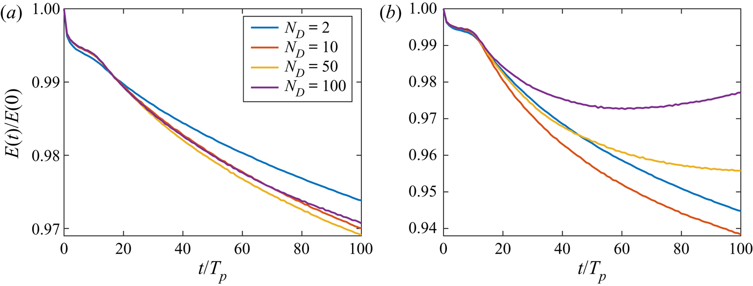
every time step. In an attempt to quantify the effect of the damping, we show the time evolution of the total mechanical energy

(3.7)\begin{equation} E = \frac{1}{2} \int_{0}^{L_y} \int_{0}^{L_x} \left( \varPhi_s \frac{\partial \eta}{\partial t} + g \eta^2 \right) \mathrm{d} x \,\mathrm{d} y \end{equation}

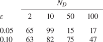
for our simulations in figure 2. The simulations are made with the values 0.05 and 0.10 for the steepness, $\varepsilon$, the values 2, 10, 50 and 100 for the parameter $N_D$ and the computational parameters listed in § 3.5. The results show that the total energy changes by roughly 2.5 %–6 % within the first 100 peak periods, and as such, the change in the total energy is comparable in magnitude to that found by Xiao et al. (Reference Xiao, Liu, Wu and Yue2013).

Figure 2.

The total mechanical energy (3.7) as a function of time for wave fields of steepness $\varepsilon = 0.05$ (a) and $\varepsilon = 0.10$ (b) for different values of $N_D$. The legend applies to both figures, and it should be noted that the $y$-axes have different scales.

3.3. Computation of $v_z^{(s)}$ given $\eta$ and $\varPhi _s$

To compute $v_z^{(s)}$ from $\eta$ and $\varPhi _s$, one must solve the Laplace equation (2.1a) together with the boundary condition (2.1b) and the condition $\varPhi |_{z = \eta } = \varPhi _s$. In the present method this is done by dividing the fluid domain into an upper part with $z > -b$ and a lower part with $z < -b$, where $b$ is a positive number such that the level $z = -b$ lies below the lowest point of the surface elevation. As has, for example, been shown by Nicholls (Reference Nicholls2011), the Laplace problem in the lower part of the domain can be solved analytically, and the full Laplace problem therefore reduces to the set of equations

(3.8a)\begin{gather} \frac{\partial^2 \varPhi}{\partial x^2} + \frac{\partial^2 \varPhi}{\partial y^2} + \frac{\partial^2 \varPhi}{\partial z^2} = 0 \quad \text{for }-b < z < \eta, \end{gather}

(3.8b)\begin{gather}\varPhi |_{z = \eta} = \varPhi_s, \end{gather}

(3.8c)\begin{gather}\left.\frac{\partial \varPhi}{\partial z}\right|_{z ={-}b} - T[\varPhi |_{z ={-}b}] = 0, \end{gather}

which is a Laplace problem on the upper part of the domain only. Here the operator $T$ is defined through its action on the function $\exp ({\textrm {i} \boldsymbol {k} \cdot \boldsymbol {r}})$, which is $T[\exp ({\textrm {i} \boldsymbol {k} \cdot \boldsymbol {r}})] = |\boldsymbol {k}| \exp ({\textrm {i} \boldsymbol {k} \cdot \boldsymbol {r}})$ for all $\boldsymbol {k}$, and we note that this is slightly different than the definition given in Klahn et al. (Reference Klahn, Madsen and Fuhrman2021a), since a finite water depth is considered there. To solve the reduced Laplace problem (3.8), the change of coordinates $(x, y, z) \mapsto (x, y, s)$ is performed with $s$ defined as

(3.9)\begin{equation} s(x,y,z) = \frac{2z + b - \eta(x,y)}{b + \eta(x,y)}. \end{equation}

Using the chain rule it follows that the function $F(x,y,s(x,y,z)) \equiv \varPhi (x,y,z)$ must satisfy the equation

(3.10)\begin{align} 0 &= \frac{\partial^2 F}{\partial x^2} + \frac{\partial^2 F}{\partial y^2} + \left( \left( \frac{\partial s}{\partial x}\right)^2 + \left( \frac{\partial s}{\partial y}\right)^2 + \left( \frac{\partial s}{\partial z}\right)^2\right) \frac{\partial^2 F}{\partial s^2} \nonumber\\ &\quad +2 \frac{\partial s}{\partial x} \frac{\partial^2 F}{\partial x \partial s} + 2 \frac{\partial s}{\partial y} \frac{\partial^2 F}{\partial y \partial s} + \left( \frac{\partial^2 s}{\partial x^2} + \frac{\partial^2 s}{\partial y^2} \right) \frac{\partial F}{\partial s}, \end{align}

as well as the boundary conditions

(3.11a)\begin{gather} F |_{s = 1} = \varPhi_s, \end{gather}

(3.11b)\begin{gather}\frac{2}{b + \eta} \left.\frac{\partial F}{\partial s}\right|_{s ={-}1} - T[F |_{s ={-}1}] = 0. \end{gather}

Finally, $F$ is computed numerically in a pseudospectral fashion by seeking the values of $F$ at the set of grid points

(3.12)\begin{equation} \left\{ (x_{n_x}, y_{n_y}, s_{n_s} )\,|\, 1 \le n_x \le 2N_x,\ 1 \le n_y \le 2N_y\ \text{and}\ 0 \le n_s \le N_s \right\}, \end{equation}

where $x_{n_x}$ and $y_{n_y}$ are given by (3.4) and $s_{n_s}$ is the $n_s$th point of the Legendre–Gauss–Lobatto quadrature of order $N_s$. To that end, $F$ is assumed to be of the form

(3.13)\begin{equation} F(x,y,s) = \sum_{n_x ={-}N_x}^{N_x-1} \sum_{n_y ={-}N_y}^{N_y-1} \sum_{n_s = 0}^{N_s} \hat{F}_{n_x, n_y, n_s} \exp ( \text{i} \boldsymbol{k}_{n_x, n_y} \cdot \boldsymbol{r} ) \mathcal{L}_{n_s}(s), \end{equation}

where $\mathcal {L}_{n_s}$ is the $n_s$th Lagrange polynomial of degree $N_s$, and (3.10) and (3.11) are required to be satisfied identically at the set of grid points (3.12). This procedure yields a system of $4N_x N_y (N_s + 1)$ linear equations for the grid point values of $F$ which is solved using the iterative method GMRES (Saad & Schultz Reference Saad and Schultz1986) with a preconditioner inspired by the work of Fuhrman & Bingham (Reference Fuhrman and Bingham2004). Once the values of $F$ at the grid points have been computed, $v_z^{(s)}$ is computed as

(3.14)\begin{equation} v_z^{(s)} = \frac{2}{b + \eta} \left.\frac{\partial F}{\partial s} \right|_{s = 1}. \end{equation}

3.4. Computation of depth-integrated quantities

In this section we show how we compute the depth-integrated quantities $\mathcal {I}_x$, $\mathcal {I}_y$, $\mathcal {D}_x$ and $\mathcal {D}_y$ numerically. As these are all of the same form and therefore can be calculated using the same procedure, we only give a detailed explanation for $\mathcal {I}_x$. For notational convenience, we will suppress any dependence on the spatial coordinates $\boldsymbol {r}$ and $z$ as well as time when these are not strictly necessary.

By the definition (1.4a,b) we have

(3.15)\begin{equation} \mathcal{I}_x= \int_{-\infty}^{\eta} a_x \,\mathrm{d} z = \underbrace{\int_{{-}b}^{\eta} a_x \,\mathrm{d} z}_{I_U} + \underbrace{\int_{-\infty}^{{-}b} a_x \,\mathrm{d} z}_{I_L}\equiv I_U + I_L, \end{equation}

where the subscripts ‘$U$’ and ‘$L$’ stand for ‘upper’ and ‘lower’, respectively. To compute the upper integral, $I_U$, we replace $z$ using the change of coordinates (3.9) and approximate the resulting integral by the same Legendre–Gauss–Lobatto quadrature used to solve the reduced Laplace problem (3.8) for $F$. This gives

(3.16)\begin{equation} I_U= \int_{{-}b}^{\eta} a_x \,\mathrm{d} z = \frac{b + \eta}{2} \int_{{-}1}^{1} a_x \,\mathrm{d} s \approx \frac{b + \eta}{2} \sum_{n_s = 0}^{N_s} w_{n_s}^{(\text{LGL})} a_x |_{z = z(s_{n_s})}, \end{equation}

in which $w_{n_s}^{(\text {LGL})}$ and $s_{n_s}$ are the $n_s$th weight and node of the Legendre–Gauss–Lobatto quadrature, respectively. To compute the lower integral, $I_L$, we follow a very similar procedure: we make the change of coordinates $z = -l/k_p - b$ and subsequently approximate the resulting integral using a Laguerre quadrature rule with $N_l$ points. This gives

(3.17)\begin{equation} I_L= \int_{-\infty}^{{-}b} a_x \,\mathrm{d} z = \frac{1}{k_p} \int_{0}^{\infty} a_x \,\mathrm{d} l \approx \frac{1}{k_p} \sum_{n_l = 1}^{N_l} (w_{n_l}^{(\text{L})} \exp(l_{n_l})) a_x |_{z = z(l_{n_l})}, \end{equation}

where $w_{n_l}^{(\text {L})}$ and $l_{n_l}$ are the $n_l$th weight and node of the Laguerre quadrature, respectively. It thus only remains for us to explain how we compute $a_x$ at the different quadrature points, and to that end, we recall that the fluid acceleration is $\boldsymbol {a} = (\partial _t + \boldsymbol {v} \boldsymbol {\cdot } \boldsymbol {\nabla }) \boldsymbol {v}$, where $\boldsymbol {\nabla } = (\partial _x, \partial _y, \partial _z)^\textrm {T}$ is the gradient in Cartesian coordinates and $\boldsymbol {v} = (v_x, v_y, v_z)^\textrm {T}$ is the fluid velocity given by $\boldsymbol {v} = \boldsymbol {\nabla } \varPhi$.

In the upper part of the fluid domain we compute the values of $a_x$ using a procedure that involves solving the reduced Laplace problem (3.8) for $F$ and the corresponding reduced Laplace problem for $G(x, y, s(x,y,z)) = \partial _t \varPhi (x,y,z)$ (see, e.g. § 2.2.3 of Klahn, Madsen & Fuhrman Reference Klahn, Madsen and Fuhrman2021b). More specifically, we compute $F$ and $G$ at the Legendre–Gauss–Lobatto quadrature points using the method described in the previous section, and then compute the acceleration field as

(3.18)\begin{equation} \boldsymbol{a} = \tilde{\boldsymbol{\nabla}} G + ( ( \tilde{\boldsymbol{\nabla}} F ) \boldsymbol{\cdot}\tilde{\boldsymbol{\nabla}} ) ( \tilde{\boldsymbol{\nabla}} F ), \end{equation}

where the operator $\tilde {\boldsymbol {\nabla }}$ is defined as $\tilde {\boldsymbol {\nabla }} = \boldsymbol {\nabla } + (\boldsymbol {\nabla } s) \partial _s$ and it is understood that $\partial _z F = \partial _z G = 0$. In the lower part of the domain we follow a rather different approach to compute the values of $a_x$ at the Laguerre quadrature points. In this approach we first compute the values of $\partial _t v_x$, $v_x$, $\partial _x v_x$, etc. at the quadrature points, before we compute the values of $a_x$ as

(3.19)\begin{equation} a_x = \frac{\partial v_x}{\partial t}+ v_x \frac{\partial v_x}{\partial x} + v_y \frac{\partial v_x}{\partial y}+ v_z \frac{\partial v_x}{\partial z}. \end{equation}

In order to compute the values of, for example, $v_x$ at the quadrature points, we utilize the fact that $v_x$ must be a solution to the Laplace equation within the fluid domain. This implies that if we write

(3.20)\begin{equation} v_x |_{z ={-}b}\equiv \tilde{\boldsymbol{\nabla}} F|_{s ={-}1} = \sum_{n_x ={-}N_x}^{N_x-1} \sum_{n_y ={-}N_y}^{N_y-1} \hat{v}_{n_x, n_y} \exp (\text{i} \boldsymbol{k}_{n_x, n_y} \cdot \boldsymbol{r}), \end{equation}

then $v_x$ must be given by the expression

(3.21)\begin{equation} v_x = \sum_{n_x ={-}N_x}^{N_x-1} \sum_{n_y ={-}N_y}^{N_y-1} \hat{v}_{n_x, n_y} \exp \left( |\boldsymbol{k}_{n_x, n_y}| (z + b) \right) \exp (\text{i} \boldsymbol{k}_{n_x, n_y} \cdot \boldsymbol{r}) \end{equation}

for $z < - b$. Clearly, we therefore have

(3.22)\begin{equation} v_x |_{z = z(l_{n_l})} = \sum_{n_x ={-}N_x}^{N_x-1} \sum_{n_y ={-}N_y}^{N_y-1} \hat{v}_{n_x, n_y} \exp \left( - \frac{|\boldsymbol{k}_{n_x, n_y}|}{k_p} l_{n_l} \right) \exp (\text{i} \boldsymbol{k}_{n_x, n_y} \cdot \boldsymbol{r}), \end{equation}

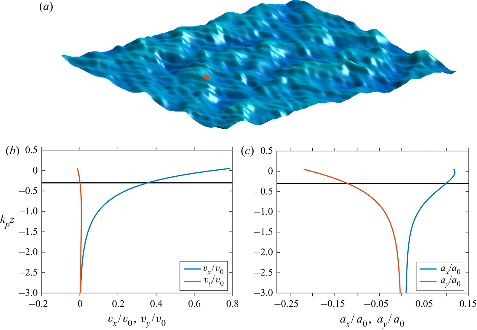
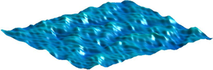
and we note that all other terms entering the right-hand side of (3.19) may be computed in a completely analogous way. For the sake of illustration, we show an example of how the surface elevation may look during the simulations as well as how the horizontal velocities and accelerations behave as a function of depth in figure 3.

Figure 3.

(a) An example of the free surface elevation in the region $\{0 \le x \le 3\lambda _p \ \text {and}\ 0 \le y \le 24 \lambda _p\}$ for the simulations with $\varepsilon = 0.10$ and $N_D = 50$ at time $t = 75 T_p$. The vertical scale is exaggerated two times. (b,c) Profiles of the horizontal velocities and accelerations below the red dot in (a). The black line shows the level $z = -b$. The computational parameters used in the simulations are listed in § 3.5, and the velocity and acceleration scales $v_0$ and $a_0$ are defined in §§ 4.2.1 and 4.1.1, respectively.

Before moving on, we note that one should be careful not to use very large values of $N_l$ in connection with this algorithm, since it becomes numerically unstable when $N_l$ becomes large. In practice we have found that when $N_l \approx 30$ in the computations, the results are converged to at least six significant digits which is sufficient for the present purpose. For larger values of $N_l$, we have, however, found the results to become increasingly inaccurate.

3.5. Computational parameters

As basic dimensional parameters of the wave fields we choose the gravitational acceleration, $g = 9.81$ m s$^{-2}$, and the peak wavelength, $\lambda _p = 275$ m (corresponding to the peak period $T_p = 13.3$ s). We characterize a wave field by its steepness $\varepsilon$ and its value of $N_D$, and in this work we simulate wave fields with $\varepsilon = 0.05$ and 0.10, and $N_D = 2$, 4, 10 and 100. For all values of $N_D$, we discretize both the $x$- and $y$-directions of all wave fields with $2N_x = 2N_y = 1024$ grid points. Since the variation of the wave fields in the $x$-direction does not depend much on $N_D$, we take $L_x = 50 \lambda _p$ in all simulations. The variation of the wave fields in the $y$-direction, however, depends strongly on $N_D$, and we therefore take

(3.23) \begin{equation} L_y= \frac{ \langle ( \partial_x \eta^{(1)} )^2 \rangle^{1/2}}{\langle ( \partial_y \eta^{(1)} )^2 \rangle^{1/2}} L_x= \frac{\left( \int_0^{2{\rm \pi}} D(\theta) \cos^2(\theta) \,\mathrm{d} \theta \right)^{1/2}}{\left(\int_0^{2{\rm \pi}} D(\theta) \sin^2(\theta) \,\mathrm{d} \theta\right)^{1/2}} L_x= ( 1 + N_D)^{1/2} L_x, \end{equation}

where $\eta ^{(1)}$ is the first-order solution to (2.1) initialized from the JONSWAP spectrum $J(\omega , \theta )$ given by (4.4a) below. This choice of $L_y$ is made in an attempt not to ‘waste’ degrees of freedom in the $y$-direction for large values of $N_D$, and we note that although the idea is rather simple, it has to our knowledge not been used in any numerical study of irregular wave fields until now.

At this stage we believe that a few comments on the spatial scales and resolution are appropriate. Since $N_x$ and $N_y$ are finite, it can be shown using the linear dispersion relation for waves in deep water that the frequency spectrum (2.2) with the present choice of $N_y$ and $L_y$ is effectively cut off at the frequency $\omega _c$, say, given by

(3.24)\begin{equation} \omega_c = \left( \frac{2 + N_D}{1 + N_D} \right)^{1/4} \left( \frac{N_x}{L_x / \lambda_p} \right)^{1/2} \omega_p. \end{equation}

As such, the cut-off frequency is determined by the directional spreading and half the number of grid points used per peak wavelength in the main direction (recall that the total number of grid points in the main direction is $2N_x$ rather than $N_x$). Since $N_x = 512$, slightly more than 20 points are used per peak wavelength, and for the values of $N_D$ used in this work, $\omega _c$ therefore lies between $3.21 \omega _p$ for $N_D = 100$ and $3.44 \omega _p$ for $N_D = 2$. Thus, it should be possible to capture the main features of the nonlinear interactions up to at least third order with the present resolution. It is of course also important that the peak of the initial spectrum is properly resolved. 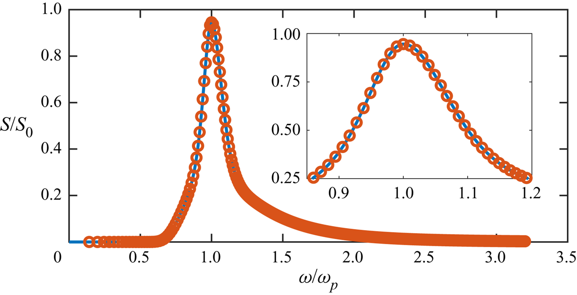To that end, we note that the choice of $L_x$ implies that the frequency resolution in the vicinity of the spectral peak is ${\rm \Delta} \omega \approx 0.01 \omega _p$ for the main direction, and from figure 4, it can be seen that this gives an accurate description of the spectral peak. Since the frequency resolution in all other directions is similar, we are content that the spatial scales and resolution used in this work are adequate for the present purpose.

Figure 4.

The frequency spectrum (2.2) (full line) compared with its discretized version when using the discrete frequencies of the main direction (circles). The inset shows the spectrum in the range $0.9 \lesssim \omega / \omega _p \lesssim 1.2$.

When solving the reduced Laplace problem (3.8), we take $b = 6 \langle \eta ^2 \rangle ^{1/2} = 3 \varepsilon \lambda _p / ( 2 {\rm \pi})$ such that the dimensionless depth of the computational domain is $k_p b = 3 \varepsilon$. This should be compared with the large, finite water depth, $h$, needed to simulate wave fields in infinite depth by similar numerical methods which solve the Laplace equation for the entire fluid domain by stretching the vertical coordinate without using the artificial boundary condition (3.8c). These methods need a computational domain with the dimensionless vertical extent $k_p h = O(2{\rm \pi} )$ in order to simulate wave fields in infinitely deep water (see the work of Barratt, Bingham & Adcock (Reference Barratt, Bingham and Adcock2020) for an example), and as such, the vertical extent of the domain of the present numerical method is therefore at least an order of magnitude smaller than that needed by similar methods. We resolve the vertical dimension using $N_s = 10$ (corresponding to 11 grid points) for all wave fields, and employ the GMRES method with the relative tolerance $10^{-6}$. The time integration of the wave fields is carried out for $0 \le t \le 100T_p$ with the time step ${\rm \Delta} t = T_p/50$, and for each combination of $\varepsilon$ and $N_D$, we have performed the time integration with 80 different random initial conditions in order to ensure a reasonably low level of statistical noise in the final results. In each of the simulations we ramp up the nonlinear interactions among the Fourier components of the wave fields using the parameters $n = 4$ and $T_R = 10T_p$.

The numerical method is implemented as a serial Matlab program, and the computational bottleneck of the method is the reduced Laplace equation which is here solved with $1024 \times 1024 \times 11 \approx 11.5 \times 10^6$ grid points four times per time step. By construction of the preconditioning strategy, the efficiency of the program varies with $\varepsilon$ and $N_D$, but in all cases the wall-clock time per time step was typically limited from above by about 4 minutes such that the 100 peak periods of simulation were each completed in about two weeks on the high performance computing cluster of the Technical University of Denmark. We note that the simulations have thus cumulatively taken about 25 years of computation time in total.

4.1. Probability density functions of $\mathcal {I}_x$ and $\mathcal {I}_y$

4.1.1. The PDF of $\mathcal {I}_x$

By the definition (1.4a,b), the depth-integrated inertia term in the $x$-direction is given by the expression

(4.7)\begin{equation} \mathcal{I}_x = \int_{-\infty}^{\eta} a_x \,\mathrm{d} z. \end{equation}

To first order in $\varepsilon$, this expression reduces to

(4.8)\begin{equation} \mathcal{I}_x = \int_{-\infty}^{0} a_x^{(1)} \,\mathrm{d} z, \end{equation}

where $a_x^{(1)} \equiv \partial _t \partial _x \varPhi ^{(1)}$ is the first-order fluid acceleration in the $x$-direction. Using (4.4b) gives

(4.9)\begin{equation} a_x^{(1)} = \sum_{n} \hat{a}_n \omega_n^2 \cos(\theta_n) \exp \left( |\boldsymbol{k}_{n}| z \right) \sin(\phi_n), \end{equation}

and, therefore, to first order in $\varepsilon$, we have

(4.10)\begin{equation} \mathcal{I}_x = g \sum_{n} \hat{a}_n \cos(\theta_n) \sin(\phi_n), \end{equation}

which follows from (4.8) and the fact that $|\boldsymbol {k}_n | = \omega _n^2/g$. Using this expression for $\mathcal {I}_x$, we now calculate the power series form of its moment generating function by directly calculating its moments. For all non-negative integers $p$, it holds that

(4.11) \begin{align} \langle \mathcal{I}_x^{2p+1} \rangle &= g^{2p+1} \sum_{n_1} \cdots \sum_{n_{2p+1}} (( \hat{a}_{n_1} \cdots \hat{a}_{n_{2p+1}} )\nonumber\\ &\quad \times ( \cos(\theta_{n_{1}}) \cdots \cos(\theta_{n_{2p+1}}) ) \langle \sin(\phi_{n_1}) \cdots \sin(\phi_{n_{2p+1}}) \rangle ) \nonumber\\ &= 0, \end{align}

since by definition of the phases the average of a product of an odd number of sine functions is zero. Thus, all odd moments vanish identically. For the even moments, we find that

(4.12) \begin{align} \langle \mathcal{I}_x^{2p} \rangle &= g^{2p} \sum_{n_1} \cdots \sum_{n_{2p}} (( \hat{a}_{n_1} \cdots \hat{a}_{n_{2p}} )\nonumber\\ &\quad \times ( \cos(\theta_{n_{1}}) \cdots \cos(\theta_{n_{2p}}) ) \langle \sin(\phi_{n_1}) \cdots \sin(\phi_{n_{2p}}) \rangle ), \end{align}

and this is zero unless the phases of the sine functions have the same indices in groups of 2, 4, 6, etc. The contributions from the groups larger than 2, however, become negligible when the set of indices is chosen such that the sum-to-integral-conversion rule (4.6) applies (see, e.g. the remark by Longuet-Higgins (Reference Longuet-Higgins1963) immediately after his (2.3)). For that reason, we find that

(4.13)\begin{equation} \langle \mathcal{I}_x^{2p} \rangle= \frac{(2p)!}{2^p p!} \left( g^2 \sum_{n} \sum_{m} \hat{a}_n \hat{a}_m \cos(\theta_n) \cos(\theta_m) \langle \sin(\phi_n) \sin(\phi_m) \rangle\right)^{p}, \end{equation}

where the numerical factor in front of the parenthesis is the number of unique pairs that can be chosen from a set of $2p$ numbers. If we now utilize the fact that $\langle \sin (\phi _n) \sin (\phi _m) \rangle = \frac {1}{2} \delta _{n,m}$, where $\delta _{n,m}$ is the Kronecker delta, we find that

(4.14)\begin{equation} \langle \mathcal{I}_x^{2p} \rangle= \frac{(2p)!}{2^p p!} \left( g^2 \sum_{n} \frac{1}{2} \hat{a}_n^2 \cos^2(\theta_n)\right)^{p}. \end{equation}

Using (4.6) as well as the definition of $\varepsilon$, it may be shown that

(4.15)\begin{equation} g^2 \sum_{n} \frac{1}{2} \hat{a}_n^2 \cos^2(\theta_n) = g^2 \int_{0}^{\infty} S(\omega) \,\mathrm{d} \omega \int_{0}^{2{\rm \pi}} D(\theta) \cos^2(\theta) \,\mathrm{d} \theta = \frac{1}{4} \frac{1 + N_D}{2 + N_D} \left(\frac{a_0}{k_p} \right)^2, \end{equation}

where $a_0 = \varepsilon g$, and clearly this implies that the even moments of $\mathcal {I}_x$ are

(4.16)\begin{equation} \langle \mathcal{I}_x^{2p} \rangle = \frac{(2p)!}{2^p p!}\left(\frac{1}{4} \frac{1 + N_D}{2 + N_D} \right)^{p} \left(\frac{a_0}{k_p} \right)^{2p}. \end{equation}

Using the one-dimensional analogue of (4.3) and a few straightforward algebraic manipulations in combination with (4.11) and (4.16) now shows that the moment generating function of $\mathcal {I}_x$ is

(4.17)\begin{align} M_{ \mathcal{I}_x}(t)=\sum_{p = 0}^{\infty} \frac{1}{p!} \left( \frac{1}{2} \left( \frac{a_0 t}{k_p} \right)^2 \left( \frac{1}{4} \frac{1 + N_D}{2 + N_D} \right) \right)^{p}= \exp \left( \frac{1}{2} \left( \frac{a_0 t}{k_p} \right)^2 \left( \frac{1}{4} \frac{1 + N_D}{2 + N_D} \right) \right), \end{align}

where the second equality follows from the fact that the infinite series is simply the Taylor expansion of an exponential function. From the remark given immediately after (4.2), it now follows that $\mathcal {I}_x/(a_0/k_p)$ is normally distributed with zero mean and variance $(1+N_D)/( 4(2+N_D) )$, and its PDF therefore reads

(4.18)\begin{equation} p \left( \frac{\mathcal{I}_x}{a_0/k_p} \right) = \left( \frac{2}{\rm \pi} \frac{2 + N_D}{1 + N_D} \right)^{1/2} \exp \left( - \frac{2(2 + N_D)}{1 + N_D} \left( \frac{\mathcal{I}_x}{a_0/k_p} \right)^2 \right). \end{equation}

Combining this result with the fact that the fraction $(2+N_D)/(1+N_D)$ decreases with $N_D$, we conclude that the probability of finding a value of $\mathcal {I}_x/(a_0/k_p)$ with large magnitude increases with the parameter $N_D$. We note that this is in line with what one would expect, as the wave motion becomes increasingly concentrated around the $x$-direction when $N_D$ becomes large.

4.1.2. The PDF of $\mathcal {I}_y$

To first order in $\varepsilon$, the PDF of $\mathcal {I}_y$ may be calculated using the exact same steps as used above. In fact, the only difference is that $a_x^{(1)}$ should be replaced by

(4.19)\begin{equation} a_y^{(1)}= \sum_{n} \hat{a}_n \omega_n^2 \sin(\theta_n) \exp \left( |\boldsymbol{k}_{n}| z \right) \sin(\phi_n) \end{equation}

in (4.8). Since the expression for $a_y^{(1)}$ is identical to that of $a_x^{(1)}$ except that it contains a sine function instead of a cosine function, the PDF of $\mathcal {I}_y/(a_0/k_p)$ can be obtained directly from (4.18) simply by replacing the fraction $(1+N_D)/(2+N_D)$ with

(4.20)\begin{equation} \int_{0}^{2{\rm \pi}} D(\theta) \sin^2(\theta) \,\mathrm{d} \theta = \frac{1}{2 + N_D}. \end{equation}

The final result for the PDF of $\mathcal {I}_y/(a_0 / k_p)$ therefore reads

(4.21)\begin{equation} p \left( \frac{\mathcal{I}_y}{a_0/k_p} \right) = \left( \frac{2}{\rm \pi} (2 + N_D) \right)^{1/2} \exp \left( - 2(2 + N_D) \left( \frac{\mathcal{I}_y}{a_0/k_p} \right)^2 \right). \end{equation}

Clearly, the tails of this PDF will decay more rapidly to 0 as $N_D$ increases, and we therefore conclude that large values of $\mathcal {I}_y$ become less probable when $N_D$ becomes large. We note that this is in line with what one would expect for the same reason as given above.

4.1.3. Comparison of (4.18) and (4.21) with simulations of wave fields for negligible $\varepsilon$

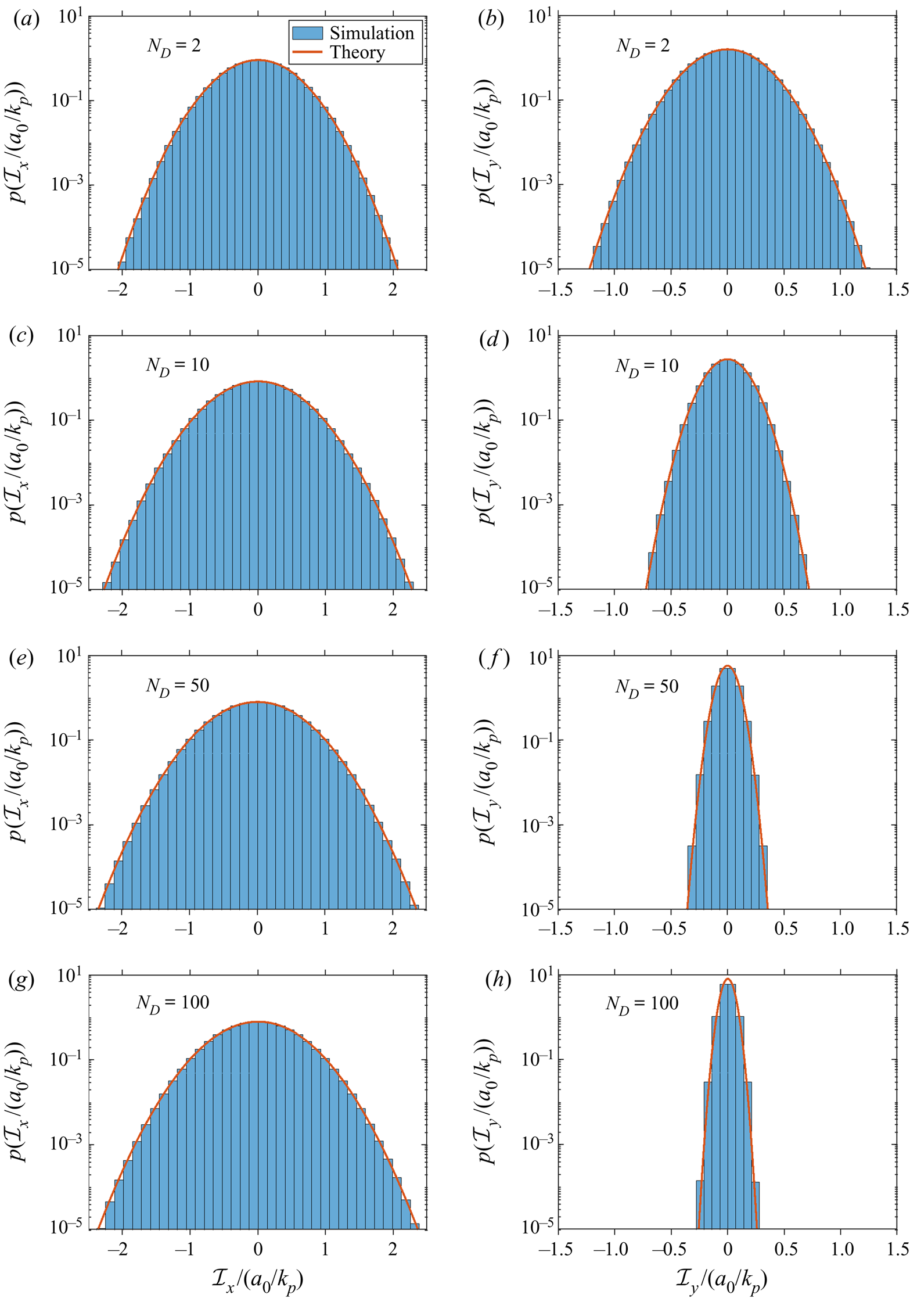
We conclude the treatment of the depth-integrated inertia terms by validating the expressions (4.18) and (4.21) against the results of simulations of wave fields with $\varepsilon = 10^{-6}$. In figure 5 a comparison between the simulated and analytical results are shown for $N_D = 2$, 10, 50 and 100, and from it we conclude that the derived expressions for $p(\mathcal {I}_x/(a_0/k_p))$ and $p( \mathcal {I}_y/(a_0/k_p))$ match the simulation results very well. In this connection it is interesting to note that while the PDF of $\mathcal {I}_x/(a_0/k_p)$ only widens slightly when $N_D$ is increased from 2 to 100, the PDF of $\mathcal {I}_y/(a_0/k_p)$ narrows significantly. As such, the statistical properties of $\mathcal {I}_y/(a_0/k_p)$ seem to be much more sensitive to changes in the directional spread of the wave field than the statistical properties of $\mathcal {I}_x/(a_0/k_p)$.

Figure 5.

A comparison of the PDFs of $\mathcal {I}_x$ (left column) and $\mathcal {I}_y$ (right column) obtained from simulation of wave fields with $\varepsilon = 10^{-6}$ with the analytical expressions (4.18) and (4.21) for different values of $N_D$. The legend applies to all figures.

4.2. Probability density functions of $\mathcal {D}_x$ and $\mathcal {D}_y$

4.2.1. A method for sampling the PDFs of $\mathcal {D}_x$ and $\mathcal {D}_y$

In the following we describe a method based on first-order theory with which random realizations of $\mathcal {D}_x$ and $\mathcal {D}_y$ can be sampled. Obviously, by binning these samples and normalizing the bin values, the PDFs of the depth-integrated drag terms can be estimated. Since the method is essentially the same for $\mathcal {D}_y$ as for $\mathcal {D}_x$, we only describe it for the latter.

The starting point of the method is the definition of $\mathcal {D}_x$ (see (1.4a,b)), i.e.

(4.22)\begin{equation} \mathcal{D}_x = \int_{-\infty}^{\eta} v_x ( v_x^2 + v_y^2 )^{1/2}\,\mathrm{d} z, \end{equation}

which, when approximated to lowest order in $\varepsilon$, becomes

(4.23)\begin{equation} \mathcal{D}_x = \int_{-\infty}^{0} v_x^{(1)} ( v_x^{(1)^2} + v_y^{(1)^2} )^{1/2}\,\mathrm{d} z. \end{equation}

Here $v_x^{(1)} \equiv \partial _x \varPhi ^{(1)}$ and $v_y^{(1)} \equiv \partial _y \varPhi ^{(1)}$ are the first-order fluid velocities in the $x$- and $y$-directions, respectively, and using (4.4b) it is straightforward to show that

(4.24a)\begin{gather} v_x^{(1)} = \sum_{n} \hat{a}_n \omega_n \cos(\theta_n) \exp \left( |\boldsymbol{k}_{n}| z \right) \cos(\phi_n), \end{gather}

(4.24b)\begin{gather}v_y^{(1)} = \sum_{n} \hat{a}_n \omega_n \sin(\theta_n) \exp \left(|\boldsymbol{k}_{n}| z \right) \cos(\phi_n). \end{gather}

To proceed from here we perform a change of coordinates, setting $z = -\alpha /k_p$ in (4.23), and approximate the resulting integral using a Laguerre quadrature rule with $N_\alpha$ points. This gives

(4.25)\begin{align} \mathcal{D}_x &= \frac{1}{k_p} \int_{0}^{\infty} v_x^{(1)} \left( v_x^{(1)^2} + v_y^{(1)^2} \right)^{1/2} \mathrm{d} \alpha \nonumber\\ &\approx \frac{1}{k_p} \sum_{n_{\alpha} = 1}^{N_\alpha} W_{n_\alpha} \left.\left( v_x^{(1)} \left( v_x^{(1)^2} + v_y^{(1)^2} \right)^{1/2} \right)\right|_{z = z(\alpha_{n_\alpha})}, \end{align}

where $W_{n_\alpha } = w_{n_\alpha } \exp (\alpha _{n_\alpha })$, and $\alpha _{n_\alpha }$ and $w_{n_\alpha }$ are the $n_\alpha$th quadrature point and weight of the Laguerre quadrature rule, respectively. We note that since $v_x^{(1)}$ and $v_y^{(1)}$ are both solutions to the Laplace equation, they depend analytically on $z$ and the quadrature therefore converges to the exact result at an exponential rate. Thus, for all practical purposes, the finite sum may be considered to be exact as long as $N_\alpha$ is moderately large. As such, we conclude that a realization of $\mathcal {D}_x$ may be computed from a realization of the vector

(4.26)\begin{equation} \boldsymbol{v} = \begin{bmatrix} v_x^{(1)} |_{z = z(\alpha_1)}, & \ldots, & v_x^{(1)} |_{z = z(\alpha_{N_\alpha})}, & v_y^{(1)} |_{z = z(\alpha_1)}, & \dots, & v_y^{(1)} |_{z = z(\alpha_{N_\alpha})} \end{bmatrix}^\textrm{T}, \end{equation}

and to complete the description of the sampling method we therefore simply need to derive the PDF of $\boldsymbol {v}$. From (4.3), it is clear that the moment generating function of $\boldsymbol {v}$ can be evaluated from the term $\langle (\boldsymbol {t}^\textrm {T} \boldsymbol {v} )^p \rangle$, for which we therefore seek an expression. Denoting the $n$th entry of $\boldsymbol {v}$ by $v_n$ and the $n$th entry of $\boldsymbol {t}$ by $t_n$, we have

(4.27)\begin{equation} \langle ( \boldsymbol{t}^\textrm{T} \boldsymbol{v} )^p \rangle = \sum_{n_1 = 1}^{2N_\alpha} \cdots \sum_{n_p = 1}^{2N_\alpha} \left( t_{n_1} \cdots t_{n_p} \right) \langle v_{n_1} \cdots v_{n_p} \rangle, \end{equation}

and from this result we immediately conclude that the term is zero whenever $p$ is odd, since the average in that case will be over an odd number of cosine functions, cf. (4.24). Substituting $p$ with $2p$, we find after a few calculations that the even terms are

(4.28)\begin{align} \langle ( \boldsymbol{t}^\textrm{T} \boldsymbol{v} )^{2p} \rangle &= \sum_{n_1 = 1}^{2N_\alpha} \cdots \sum_{n_{2p} = 1}^{2N_\alpha}(t_{n_1} \cdots t_{n_{2p}}) \langle v_{n_1} \cdots v_{n_{2p}}\rangle\nonumber\\ &= \frac{(2p)!}{2^p p!} \left( \sum_{n = 1}^{2N_\alpha} \sum_{m = 1}^{2N_\alpha} t_n t_m \langle v_n v_m \rangle \right)^{p}. \end{align}

If we now define the matrix $\boldsymbol \varSigma _v$ such that its $(n,m)$th entry is $\langle v_n v_m \rangle$, the results for the even and odd terms imply that the moment generating function of $\boldsymbol {v}$ is

(4.29)\begin{equation} M_{\boldsymbol{v}}(\boldsymbol{t}) = \sum_{p = 0}^{\infty} \frac{1}{(2p)!} \langle \left( \boldsymbol{t}^\textrm{T} \boldsymbol{v} \right)^{2p} \rangle = \sum_{p = 0}^{\infty} \frac{1}{p!} \left( \frac{1}{2} \boldsymbol{t}^\textrm{T} \boldsymbol\varSigma_v \boldsymbol{t} \right)^p = \exp \left( \frac{1}{2} \boldsymbol{t}^\textrm{T} \boldsymbol\varSigma_v \boldsymbol{t} \right), \end{equation}

and when combined with the remark given immediately after (4.2), this result implies that $\boldsymbol {v}$ follows a multivariate normal distribution with covariance matrix $\boldsymbol \varSigma _v$. We note that samples of such a distribution may nowadays be generated efficiently by a wide variety of software packages, and to complete the description of the sampling method it therefore suffices to construct the covariance matrix of $\boldsymbol {v}$. For arbitrary $n$ and $m$, it may be shown that $\langle v_x^{(1)} |_{z = z(\alpha _n)} v_y^{(1)} |_{z = z(\alpha _m)} \rangle = 0$, and as a consequence, the covariance matrix simplifies to

(4.30)\begin{equation} \boldsymbol\varSigma_v =\begin{bmatrix} \boldsymbol\varSigma_{v_x} & \boldsymbol{0} \\ \boldsymbol{0} & \boldsymbol\varSigma_{v_y} \end{bmatrix}. \end{equation}

Here $\boldsymbol \varSigma _{v_x} \equiv \langle \boldsymbol {v}_x \boldsymbol {v}_x^\textrm {T} \rangle$ and $\boldsymbol \varSigma _{v_y} \equiv \langle \boldsymbol {v}_y \boldsymbol {v}_y^\textrm {T} \rangle$ are the covariance matrices of the vectors

(4.31a)\begin{gather} \boldsymbol{v}_x = \begin{bmatrix} v_x^{(1)} |_{z = z(\alpha_1)}, & \ldots, & v_x^{(1)} |_{z = z(\alpha_{N_\alpha})} \end{bmatrix}, \end{gather}

(4.31b)\begin{gather}\boldsymbol{v}_y = \begin{bmatrix} v_y^{(1)} |_{z = z(\alpha_1)}, & \ldots, & v_y^{(1)} |_{z = z(\alpha_{N_\alpha})} \end{bmatrix}. \end{gather}

Using (4.6) these matrices may be shown to be given by the expressions

(4.32a,b)\begin{equation} \boldsymbol\varSigma_{v_x} = v_0^2 \frac{1+N_D}{2+N_D} \boldsymbol\varSigma,\quad \text{and}\quad \boldsymbol\varSigma_{v_y} = v_0^2 \frac{1}{2+N_D} \boldsymbol\varSigma, \end{equation}

where $v_0 \equiv \varepsilon (g/k_p)^{1/2}$ and the matrix $\boldsymbol \varSigma$ is defined such that its $(n,m)$th entry is

(4.33)\begin{equation} \boldsymbol\varSigma_{n,m}= \frac{\displaystyle \int_{0}^{\infty} \exp \left( - x^2(\alpha_n + \alpha_m) \right) x^{{-}3} \exp \left( - \frac{5}{4} x^{{-}4} \right) \gamma^{\exp ( - ({(x - 1)^2}/{2\sigma^2}))}\,\mathrm{d} x}{ \displaystyle 4 \int_{0}^{\infty} x^{{-}5} \exp \left( - \frac{5}{4} x^{{-}4} \right) \gamma^{\exp ( - ({(x - 1)^2}/{2\sigma^2}))}\,\mathrm{d} x}, \end{equation}

in which $\gamma$ and $\sigma$ are parameters of the frequency spectrum (2.2). This concludes the description of the sampling method.

4.2.2. An asymptotic result for the PDF of $\mathcal {D}_x$

We now derive an analytical expression for the PDF of $\mathcal {D}_x$, and because the derivation is somewhat more complicated than those presented above, we divide it into three steps. In the first step, the PDF of $\mathcal {D}_x$ is related to that of $| \mathcal {D}_x |$, and the latter is approximated by a finite sum. In the second step, the finite sum is rewritten as a linear combination of independent random variables, from which the moment generating function is calculated. Finally, in the third step, this function is inverted using the inverse Laplace transform.

Our derivation starts from (4.23), which we rewrite as

(4.34)\begin{equation} \mathcal{D}_x = \int_{-\infty}^{0} v_x^{(1)} | v_x^{(1)} | \left( 1 + \left( \frac{v_y^{(1)}}{v_x^{(1)}}\right)^2 \right)^{1/2} \mathrm{d} z. \end{equation}

From (4.32a,b), it follows that at any fixed depth we have $( v_y^{(1)}/v_x^{(1)} )^2 = O( (1+N_D)^{-1} )$ in a statistical sense, and neglecting the square root factor of the integrand thus introduces an error which on average is proportional to $(1+N_D)^{-1}$. For long-crested wave fields, for which $N_D$ is large, this error is small, and we therefore make the approximation

(4.35)\begin{equation} \mathcal{D}_x \approx \int_{-\infty}^{0} v_x^{(1)} | v_x^{(1)} | \,\mathrm{d} z, \end{equation}

while keeping in mind that the final result will formally only be valid in the limit of large $N_D$. It follows from the results of the previous section that $v_x^{(1)}$ is a Gaussian process with zero mean when considered as a function of $z$. The symmetry of this process around 0 implies that the PDF of $\mathcal {D}_x$ is symmetrical around 0, and we may hence write

(4.36)\begin{equation} p\left( \mathcal{D}_x \right) = \tfrac{1}{2} p \left( | \mathcal{D}_x | \right). \end{equation}

We note that this relation could also have been guessed from pure physical reasoning, as the velocity of the water in the $x$-direction at any given $z$-level is known to be positive as often as negative when described with first-order theory. The relation (4.36) implies that we can restrict our attention to computing the PDF of $| \mathcal {D}_x |$, and from (4.35) we have

(4.37)\begin{equation} | \mathcal{D}_x |\approx \left| \int_{-\infty}^{0} v_x^{(1)} | v_x^{(1)} | \,\mathrm{d} z \right| \approx \int_{-\infty}^{0} v_x^{(1)^2} \,\mathrm{d} z, \end{equation}

where the approximation comes from the fact that $v_x^{(1)}$ may change sign with depth. We simplify the expression for $| \mathcal {D}_x |$ further by employing the same Laguerre quadrature as in section (4.2.1), and find that

(4.38)\begin{equation} | \mathcal{D}_x | \approx \frac{1}{k_p} \int_{0}^{\infty} v_x^{(1)^2} \,\mathrm{d} \alpha \approx \left.\frac{1}{k_p} \sum_{n_{\alpha} = 1}^{N_\alpha} W_{n_\alpha} v_x^{(1)^2} \right|_{z = z(\alpha_{n_\alpha})}. \end{equation}

For clarity, we recall that $W_{n_\alpha } = w_{n_\alpha } \exp (\alpha _{n_\alpha })$, and that $\alpha _{n_\alpha }$ and $w_{n_\alpha }$ are the $n_\alpha$th quadrature point and weight of the Laguerre quadrature rule, respectively. This completes the first part of the derivation.

In order to calculate the moment generating function of $| \mathcal {D}_x |$ we seek to rewrite (4.38) as a linear combination of squares of independent normally distributed random variables with zero mean and unit variance. To that end, we note that the vector $\boldsymbol {v}_x$ defined in (4.31) consists of correlated normal random variables and that its covariance matrix $\boldsymbol \varSigma _{v_x}$ defined in (4.32a,b) is symmetric positive-semidefinite (SPD) by construction. The latter of these facts enables us to define the dimensionless vector $\boldsymbol {X} = \boldsymbol \varSigma _{v_x}^{-1/2} \boldsymbol {v}_x$, with $\boldsymbol \varSigma _{v_x}^{1/2}$ the SPD square root of $\boldsymbol \varSigma _{v_x}$, and we may therefore rewrite (4.38) as

(4.39) \begin{equation} | \mathcal{D}_x |\approx \frac{1}{k_p} \boldsymbol{X}^\textrm{T} ( \boldsymbol\varSigma_{v_x}^{1/2} \boldsymbol{\mathsf{W}} \boldsymbol\varSigma_{v_x}^{1/2}) \boldsymbol{X}= \frac{v_0^2}{k_p} \frac{1 + N_D}{2 + N_D} \boldsymbol{X}^\textrm{T} ( \boldsymbol\varSigma^{1/2} \boldsymbol{\mathsf{W}} \boldsymbol\varSigma^{1/2}) \boldsymbol{X}. \end{equation}

Here $\boldsymbol{\mathsf{W}}$ is the diagonal matrix whose $(n,n)$th entry is $W_n$, and the second equality follows from using (4.32a,b). The symmetry of $\boldsymbol \varSigma ^{1/2}$ implies that the matrix $\boldsymbol \varSigma ^{1/2} \boldsymbol{\mathsf{W}} \boldsymbol \varSigma ^{1/2}$ is also symmetric and can therefore be orthogonally diagonalized, meaning that it can be factored as $\boldsymbol{\mathsf{P}}^\textrm {T} \boldsymbol \varLambda \boldsymbol{\mathsf{P}}$, where $\boldsymbol{\mathsf{P}}$ and $\boldsymbol \varLambda$ are orthogonal and diagonal matrices, respectively. By setting $\boldsymbol {Y} = \boldsymbol {P} \boldsymbol {X}$ and using this result in (4.39), we arrive at the relation

(4.40)\begin{equation} | \mathcal{D}_x |\approx \frac{v_0^2}{k_p} \frac{1 + N_D}{2 + N_D} \boldsymbol{Y}^\textrm{T} \boldsymbol\varLambda \boldsymbol{Y} = \frac{v_0^2}{k_p} \sum_{n_{\alpha} = 1}^{N_\alpha} \left( \frac{1 + N_D}{2 + N_D} \varLambda_{n_\alpha} \right) Y_{n_\alpha}^2, \end{equation}

which we claim is a linear combination of squared uncorrelated normally distributed variables with zero mean and unit variance. To prove this assertion, we first note that $\boldsymbol {Y} = \boldsymbol{\mathsf{P}} \boldsymbol \varSigma _{v_x}^{-1/2} \boldsymbol {v}_x$ is in fact normally distributed, since it is a linear transformation of the vector $\boldsymbol {v}_x$ which is normally distributed. Secondly, a straightforward calculation shows that $\langle \boldsymbol {Y} \rangle = \boldsymbol {0}$ and that $\langle \boldsymbol {Y} \boldsymbol {Y}^\textrm {T} \rangle$ is the identity matrix, and in combination these three results imply the desired conclusion. If we now define $\mu _{n_\alpha } = 2 (1 + N_D)/(2+ N_D) \varLambda _{n_\alpha }$ and set $\xi = | \mathcal {D}_x |/(v_0^2 / k_p)$, then from (4.40),

(4.41)\begin{equation} \xi \approx \sum_{n_\alpha = 1}^{N_\alpha} \frac{1}{2} \mu_{n_\alpha} Y_{n_\alpha}^2. \end{equation}

When combined with the facts that the components of $\boldsymbol {Y}$ are independent and all have identical PDFs, namely $p(Y_{n_\alpha }) = (2{\rm \pi} )^{-1/2} \exp ( - Y_{n_\alpha }^2/2)$, this result implies that the moment generating function of $\xi$, when evaluated at $-t$, is

(4.42)\begin{align} M_\xi ({-}t) &\approx \left\langle \exp \left( - \sum_{n_\alpha = 1}^{N_\alpha} \frac{1}{2} \mu_{n_\alpha} Y_{n_\alpha}^2 t \right) \right\rangle \nonumber\\ &= \prod_{n_\alpha = 1}^{N_\alpha} \left\langle \exp \left( - \frac{1}{2} \mu_{n_\alpha} Y_{n_\alpha}^2 t \right) \right\rangle = \prod_{n_\alpha = 1}^{N_\alpha} \frac{1}{( 1 + \mu_{n_\alpha} t)^{1/2}}. \end{align}

The PDF of $\xi$ must therefore satisfy the relation

(4.43)\begin{equation} \int_{0}^{\infty} \exp \left( - \xi t \right) p(\xi) \,\mathrm{d} \xi \approx \prod_{n_\alpha = 1}^{N_\alpha} \frac{1}{(1 + \mu_{n_\alpha} t)^{1/2}}, \end{equation}

and this completes the second part of the derivation.

At this stage the only thing left to do is to invert the relation (4.43) for $p(\xi )$. To do so, we start by considering the eigenvalues $\varLambda _{n_\alpha }$, which are given to six significant digits in table 1. From the table we see that the eigenvalues decay extremely rapidly with $n_\alpha$, such that the approximation is very accurate even for $N_\alpha$ as small as, say, 5. Moreover, the eigenvalues are all positive, and this implies that the singularities on the right-hand side of (4.43) all are located on the negative real axis. As such, $p(\xi )$ may be expressed as

(4.44)\begin{equation} p(\xi) \approx \frac{1}{2 {\rm \pi}\text{i}} \lim_{R \rightarrow \infty} \int_{ - \text{i} R}^{\text{i} R}\frac{ \exp\left( \xi t \right)}{\left( 1 + \mu_1 t \right)^{1/2} \left( 1 + \mu_2 t \right)^{1/2} \cdots ( 1 + \mu_{N_L} t )^{1/2}}\,\mathrm{d} t, \end{equation}

by using the complex inversion formula for the Laplace transform (see, e.g. Spiegel Reference Spiegel1965). To calculate this integral, we take the branch cut of the square root to be the negative part of the real line and consider the contour integral

(4.45)\begin{align} & \int_{\varGamma} \frac{ \exp\left( \xi z \right)}{\left( 1 + \mu_1 z \right)^{1/2} \left( 1 + \mu_2 z \right)^{1/2} \cdots ( 1 + \mu_{N_\alpha} z )^{1/2}}\,\mathrm{d} z \nonumber\\ &\quad =\sum_{n = 1}^{6} \int_{\varGamma_n} \frac{ \exp\left( \xi z \right)}{\left( 1 + \mu_1 z \right)^{1/2} \left( 1 + \mu_2 z \right)^{1/2} \cdots ( 1 + \mu_{N_\alpha} z )^{1/2}}\, \mathrm{d} z, \end{align}

where the components of the contour $\varGamma$ are shown in figure 6, and should be considered in the limits $R \rightarrow \infty$ and $r \rightarrow 0$. Since the integrand is holomorphic in the region inside $\varGamma$, the residue theorem (see, e.g. Berg Reference Berg2013) implies that the integral along the entire curve vanishes identically. Moreover, the contribution from $\varGamma _1$ clearly gives $2{\rm \pi} \textrm {i} p(\xi )$, and it can be shown that the contributions from $\varGamma _2$, $\varGamma _4$ and $\varGamma _6$ to the integral tend to 0 when $R$ and $r$ tend to $\infty$ and $0$, respectively. In total, we can therefore rewrite (4.45) as

(4.46)\begin{align} p(\xi) &\approx \frac{\textrm{i}}{2{\rm \pi}} \left(\int_{\varGamma_3} \frac{ \exp\left( \xi z \right)}{\left( 1 + \mu_1 z \right)^{1/2} \left( 1 + \mu_2 z \right)^{1/2} \cdots ( 1 + \mu_{N_L} z )^{1/2}}\,\mathrm{d} z \right.\nonumber\\ &\quad \left.+ \int_{\varGamma_5} \frac{ \exp\left( \xi z \right)}{\left( 1 + \mu_1 z \right)^{1/2} \left( 1 + \mu_2 z \right)^{1/2} \cdots ( 1 + \mu_{N_L} z )^{1/2}}\,\mathrm{d} z \right), \end{align}

and upon utilizing that the square root carries the opposite sign on $\varGamma _3$ than on $\varGamma _5$, we find that

(4.47)\begin{align} p(\xi) &\approx \frac{\text{i}}{2{\rm \pi}} \sum_{n = 1}^{N_\alpha} \left( ( ( -\text{i})^n - \text{i}^n) \vphantom{\int_{\mu_n^{{-}1}}^{\mu_{n+1}^{{-}1}}}\right.\nonumber\\ &\quad \times\left. \int_{\mu_n^{{-}1}}^{\mu_{n+1}^{{-}1}} \frac{\exp(-\xi t)}{\left( \mu_1 t -1 \right)^{1/2} \cdots \left( \mu_n t -1 \right)^{1/2} \left( 1 - \mu_{n+1} t \right)^{1/2} \cdots ( 1 - \mu_{N_L} t )^{1/2}}\,\mathrm{d} t \right), \end{align}

where $\mu _{N_\alpha + 1}^{-1} \equiv \infty$. The integrals inside the sum have, as we will now show, very simple asymptotic forms with which the total expression may be simplified significantly. Using Watson's lemma (see e.g. Holmes Reference Holmes2013) it can be shown that

(4.48)\begin{align} & \int_{\mu_n^{{-}1}}^{\mu_{n+1}^{{-}1}} \frac{\exp(-\xi t)}{\left( \mu_1 t -1 \right)^{1/2} \cdots \left( \mu_n t -1 \right)^{1/2} \left( 1 - \mu_{n+1} t \right)^{1/2} \cdots ( 1 - \mu_{N_L} t )^{1/2}}\,\mathrm{d} t \nonumber\\ &\quad \sim C_n \left( \frac{\rm \pi}{\mu_1 \xi} \right)^{1/2} \exp (- \mu_n^{{-}1} \xi) \end{align}

as $\xi \rightarrow \infty$, where the number $C_n$ is given by the expression

(4.49)\begin{align} C_n = \left( \frac{\varLambda_1}{\varLambda_n} -1 \right)^{{-}1/2} \cdots \left( \frac{\varLambda_{n-1}}{\varLambda_n} -1 \right)^{{-}1/2} \left( 1 - \frac{\varLambda_{n+1}}{\varLambda_n} \right)^{{-}1/2} \cdots \left( 1 - \frac{\varLambda_{N_\alpha}}{\varLambda_n} \right)^{{-}1/2}. \end{align}

If we then combine (4.36), (4.47) and (4.48) with the definitions of $\xi$ and $\mu _n$, we finally find that

(4.50)\begin{equation} p \left( \frac{\mathcal{D}_x}{v_0^2 / k_p} \right) \sim C_1 \left( 8 {\rm \pi}\varLambda_1 \frac{1 + N_D}{2 + N_D} \frac{| \mathcal{D}_x |}{v_0^2 / k_p} \right)^{{-}1/2} \exp \left( - \frac{1}{2 \varLambda_1} \frac{2 + N_D}{1 + N_D} \frac{| \mathcal{D}_x |}{v_0^2 / k_p} \right) \end{equation}

as $| \mathcal {D}_x |/(v_0^2 / k_p) \rightarrow \infty$, which concludes our derivation of the PDF of $\mathcal {D}_x$. From the asymptotic result (4.50) we conclude that when $| \mathcal {D}_x |/(v_0^2 / k_p)$ is large, it tends to follow a (scaled) chi-square distribution with one degree of freedom. We note that this result could have been anticipated qualitatively from (4.41) by combining the fact that the first term in the sum (when considered in isolation) follows a chi-square distribution with one degree of freedom with the fact that it is this term which, in some sense, is responsible for generating the events with large $| \mathcal {D}_x |/(v_0^2 / k_p)$, as it has the largest variance.

Figure 6.

The contour $\varGamma = \cup _{n = 1}^6 \varGamma _n$, which should be considered in the limits where $R$ tends to $\infty$ and $r$ tends to $0$. Here $\varGamma _1$ is a straight line from $- \text {i} R$ to $\text {i} R$, $\varGamma _2$ is a quarter circle from $\text {i} R$ to $-R$, $\varGamma _3$ is a straight line from $-R$ to $t_1$, $\varGamma _4$ is a half-circle with centre $t_1$ and radius $r$, $\varGamma _5$ is a straight line from $t_1$ to $-R$ and $\varGamma _6$ is a quarter circle from $-R$ to $- \text {i}R$. The numbers $z_1 = -\mu _1^{-1}$, $z_2 = -\mu _2^{-1}$,…, $z_{N_\alpha } = - \mu _{N_\alpha }^{-1}$ are the singularities of the integrand (4.45).

Table 1.

The eigenvalues $\varLambda _{n_\alpha }$ of the matrix $\boldsymbol \varSigma ^{1/2} \boldsymbol{\mathsf{W}} \boldsymbol \varSigma ^{1/2}$ in descending order converged to six significant digits. The eigenvalues with $n_\alpha > 6$ are all smaller than $10^{-6}$.

From the asymptotic result (4.50), it is clear that the PDF of $\mathcal {D}_x$ decays less rapidly to zero when $N_D$ increases. We therefore conclude that events where $| \mathcal {D}_x |$ is large become more probable when the directional spread of the wave field is small, as one would expect.

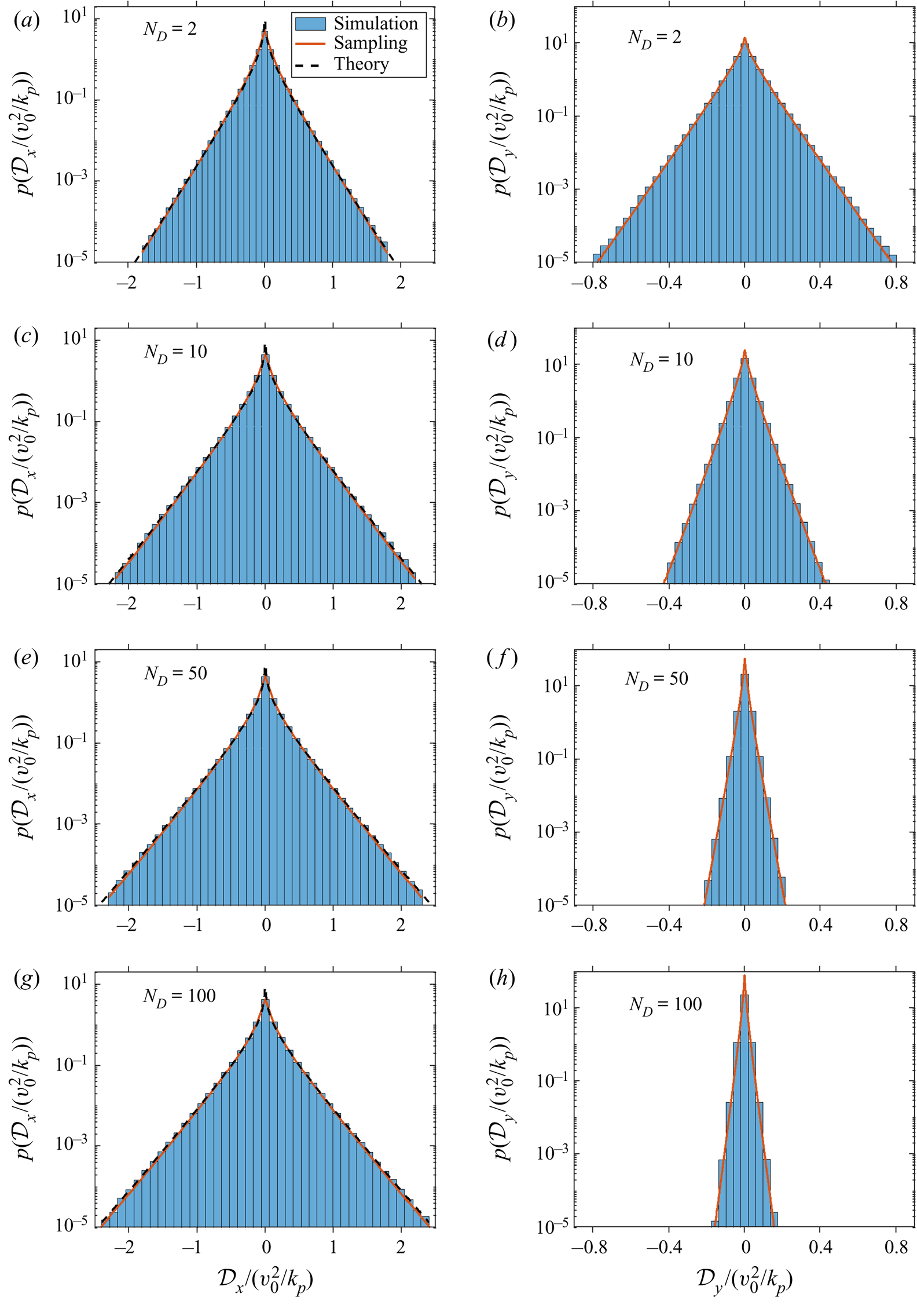
4.2.3. Comparison of the sampling method and the asymptotic approximation (4.50) with simulations of wave fields for negligible $\varepsilon$

We conclude the treatment of the depth-integrated drag terms by validating the derived results against simulations of wave fields with $\varepsilon = 10^{-6}$. For $N_\alpha = 5$ and $N_D = 2$, 10, 50 and 100, the simulated and derived results are compared in figure 7, from which it is clear that the sampling method provides a highly accurate result even when using only five points in the quadrature (4.25). The asymptotic result (4.50) in general also provides a very good match for the simulated results for all values of $N_D$, except for close to $\mathcal {D}_x/(v_0^2 / k_p) = 0$ where it diverges due to an inverse square root singularity. This is remarkable not only because of the small value of $N_\alpha$, but also because of the many approximations which have been made throughout the derivation of (4.50). In this connection one may, of course, wonder whether an even better match could be found by using the formally more accurate expression (4.47). We have tested this by evaluating (4.47) numerically, but the result does not provide a better match, since it approaches 0 as $\mathcal {D}_x$ becomes small. The reason for this behaviour is the approximation (4.37), which effectively excludes the possibility that $\mathcal {D}_x = 0$.

Figure 7.

A comparison of the PDFs of $\mathcal {D}_x$ (a,c,e,g) and $\mathcal {D}_y$ (b,d,f,h) obtained from simulation of wave fields with $\varepsilon = 10^{-6}$ with the results of the sampling method described in § 4.2.1 and the analytical expression (4.50) for different values of $N_D$. The sampling method and the analytic result have both been evaluated using $N_\alpha = 5$. The legend applies to all figures.

In addition to providing a measure for the accuracy of the derived PDFs, we note that figure 7 also illustrates the effect of the directional spread on $p( \mathcal {D}_x/(v_0^2/k_p) )$ and $p (\mathcal {D}_y/(v_0^2/k_p) )$. To that end, we conclude that the statistical properties of the depth-integrated drag terms exhibit the same qualitative behaviour as the statistical properties of the depth-integrated inertia terms in the sense that while the PDF of $\mathcal {D}_x/(v_0^2/k_p)$ only widens slightly as $N_D$ is increased from 2 to 100, the PDF of $\mathcal {D}_y/(v_0^2/k_p)$ narrows significantly.

5.1. Time of measurement

At the start of the simulations, the components of the wave fields considered in this work have finite amplitudes but uncorrelated, random phases. As such, the statistical properties of the wave fields are expected to vary considerably over the first $O(\varepsilon ^{-2})$ peak periods (see, e.g. Dysthe et al. Reference Dysthe, Trulsen, Krogstad and Socquet-Juglard2003; Annenkov & Shrira Reference Annenkov and Shrira2009; Xiao et al. Reference Xiao, Liu, Wu and Yue2013), which we note corresponds roughly to the length of our simulations. Specifically, these statistical variations relate to the skewness and kurtosis, i.e. the quantities

(5.1a,b)\begin{equation} \mathcal{S} = \frac{\langle \eta^3 \rangle}{\langle \eta^2 \rangle^{3/2}}\quad \text{and}\quad \mathcal{K} = \frac{\langle \eta^4 \rangle}{\langle \eta^2 \rangle^2}. \end{equation}

These quantities respectively take the values 0 and 3 in the case of a linear wave field, and can therefore be used as a measure of the degree of nonlinearity of the wave field. Our results for the skewness and kurtosis are shown in figure 8, from which it can be seen that $\mathcal {S}$ in all cases quickly reaches an almost constant level while $\mathcal {K}$ does not. At the instance of maximum kurtosis, the wave fields may therefore be considered to be in their most nonlinear state during the simulations, and we therefore choose to measure the statistical properties of the depth-integrated quantities at this time. In this connection we note that Toffoli et al. (Reference Toffoli, Gramstad, Truelsen, Monbaliu, Bitner-Gregersen and Onorato2010) used the same instance in time for their measurement of the PDF of the surface elevation. For completeness, the time of measurement for the different values of $\varepsilon$ and $N_D$ is listed in table 2.

Figure 8.

The time evolution of the skewness (a,c,e,g) and kurtosis (b,d,f,h) for $\varepsilon = 0.05$ and 0.10 and $N_D = 2$, 10, 50 and 100. The legend applies to all figures.

Table 2.

The dimensionless time $t/T_p$ at which the PDFs of the depth-integrated quantities are measured as a function of $\varepsilon$ and $N_D$. At the times listed, the kurtosis of the surface elevation reaches it maximum during the simulations.

5.2. The decay of kinematic quantities with depth

Although this study is mainly focused on the statistical properties of the depth-integrated inertia and drag forces, we here report on the depth variation of the forces per unit vertical length. This variation is important for at least two reasons, the first being that it can be used to qualitatively explain the behaviour of the PDFs of $D_x$ and $D_y$, and the second being that knowledge about the magnitude of the contributions to the total force at different depths is very useful for practical purposes. In deep water, which is assumed throughout this work, most offshore structures such as tension-leg platforms do not extend all the way to the seabed. As such, the total force calculated in this work presents an upper bound for the force on such structures, and how useful this bound is in practice obviously depends on whether substantial contributions to the force are found at great depth.

To quantify this, we have calculated the standard deviations of $a_x$, $a_y$, $v_x ( v_x^2 + v_y^2 )^{1/2}$ and $v_y ( v_x^2 + v_y^2 )^{1/2}$ at the time of maximum kurtosis. As mentioned above, these quantities represent the inertia and drag forces per unit vertical length, respectively. The results for $\varepsilon = 0.10$ and $N_D = 2$, 10, 50 and 100 are shown in figure 9, and from this it is clear that both the contributions to the inertia and drag force decay extremely rapidly with depth. We have found similar results for $\varepsilon = 0.05$ and, therefore, conclude that significant contributions to the inertia force are limited to the region $z \gtrsim - \lambda _p$, and that substantial contributions to the drag force are limited to the region $z \gtrsim - \lambda _p/2$. If a structure penetrates deeper into the water than a single peak wavelength, the results for the depth-integrated force in this work will thus provide an accurate estimate on the total inline force on the structure. On the other hand, if the vertical extent of the structure is less than a peak wavelength, the results of this work can only be used as an upper bound.

Figure 9.

The variation of the standard deviations of (a) $a_x$, (b) $a_y$, (c) $v_x ( v_x^2 + v_y^2 )^{1/2}$ and (d) $v_y ( v_x^2 + v_y^2 )^{1/2}$ with depth for $\varepsilon = 0.10$ and different values of $N_D$. The results are computed at the time of maximum kurtosis and the legend applies to all figures.

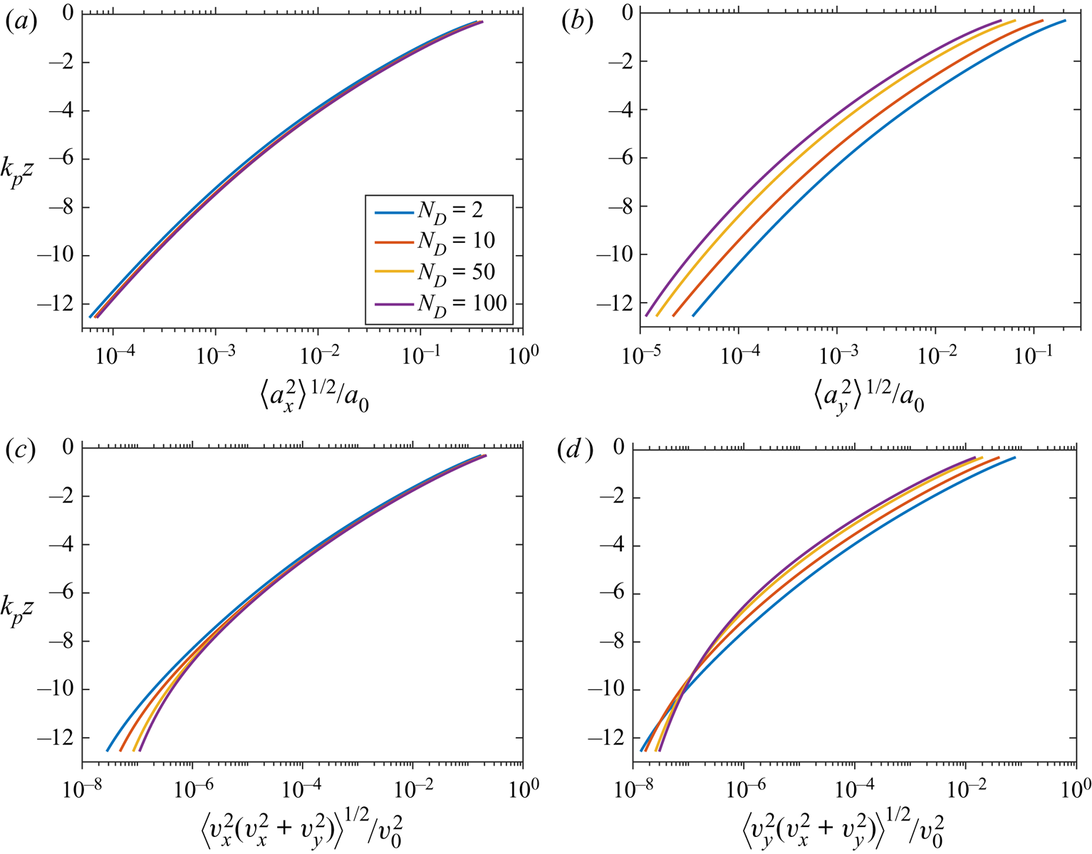
5.3. The PDF of $\mathcal {I}_x$

In figure 10 we show a comparison of the PDF of $\mathcal {I}_x$ obtained from the nonlinear simulations together with the first-order result (4.18). From the figure, it is clear that the first-order result matches the nonlinear PDF almost perfectly for all values of $\varepsilon$ and $N_D$, and this hints that the statistical properties of $\mathcal {I}_x$ are unaffected by nonlinear effects. In appendix A we present a proof of the fact that the contributions from second-order nonlinearities to the PDFs of both $\mathcal {I}_x$ and $\mathcal {I}_y$ vanish identically regardless of the shape of the underlying frequency and directional spectrum. As a consequence, the exact PDF of these quantities can only differ from the first-order result if they are affected by third- or higher-order nonlinear interactions, and for $\mathcal {I}_x$, this is clearly not the case for the range of parameters investigated here. We note that this finding may be of great practical value, since it hints that the result of the depth-integrated Morison equation (without the extensions due to, for example, Rainey Reference Rainey1989) in many cases may be accurately approximated by the normal distribution (4.18), specifically, as may be seen from (1.2), when the parameter $\mathcal {P}$ is close to zero. We return to this finding when discussing the PDF of $F^\ast$ in § 6.

Figure 10.

A comparison of the PDF of $\mathcal {I}_x$ obtained from fully nonlinear simulations at the time of maximum kurtosis with the first-order result (4.18) for different values of $\varepsilon$ and $N_D$. The legend applies to all figures.

5.4. The PDF of $\mathcal {I}_y$

Our results for the PDF of $\mathcal {I}_y$ from the nonlinear simulations are shown in figure 11 together with the first-order result given by (4.21). For $\varepsilon = 0.05$ there is a very good agreement between the nonlinear PDFs and the first-order approximation for all values of $N_D$, and this is in line with the fact that the statistical properties of $\mathcal {I}_y$ are not affected by second-order effects, cf. appendix A. For $\varepsilon = 0.10$ there is likewise a very good agreement between the exact nonlinear PDFs and the first-order approximation for $N_D = 2$ and 10, but for $N_D = 50$ and 100, the linear and nonlinear results deviate visibly as the tails of the nonlinear PDF decay much more slowly to zero. This is a clear indication of the fact that the statistical properties of $\mathcal {I}_y$ are affected by third-order nonlinearities when the steepness is appreciable and the wave field becomes long crested. We note that this finding is consistent with the results of, for example, Onorato et al. (Reference Onorato2009) and Toffoli et al. (Reference Toffoli, Gramstad, Truelsen, Monbaliu, Bitner-Gregersen and Onorato2010), who found that the PDF of the surface elevation is only affected by third-order interactions in the case where the directional spread of the wave field is relatively small.

Figure 11.

A comparison of the PDF of $\mathcal {I}_y$ obtained from fully nonlinear simulations at the time of maximum kurtosis with the first-order result (4.21) for different values of $\varepsilon$ and $N_D$. The legend applies to all figures.

5.5. The PDF of $\mathcal {D}_x$

Figure 12 shows our results for the PDF of $\mathcal {D}_x$ from the nonlinear simulations together with the results of the first-order sampling method presented in 4.2.1 when executed with $N_\alpha = 5$. From the figure, it can be seen that the first-order PDF does not provide an accurate description of the nonlinear PDF for any of the pairs $(\varepsilon ,N_D)$ used in this study. Assuming that third-order effects only come into play when $N_D$ is large, we therefore conclude that $\mathcal {D}_x$ is in general affected by second-order nonlinearities by a simple contradiction argument. To understand this result we recall that by definition

(5.2)\begin{equation} \mathcal{D}_x = \int_{-\infty}^{\eta} v_x (v_x^2 + v_y^2)^{1/2}\,\mathrm{d} z, \end{equation}

and owing to figure 9c as well as the fact that $N_D > 0$ in this study, we conclude that the dominant contribution to $\mathcal {D}_x$ comes from $v_x$ close to the surface. As has been shown by Song & Wu (Reference Song and Wu2000) for arbitrary depth, this quantity is in general affected by second-order nonlinearities (consider, for example, their (68) in the limit of large $k_p h$). In particular, Reference Song and WuSong & Wu show that the PDF of $v_x$ becomes skewed to second order, and it may be checked by numerical calculations that the skewness is positive for all cases presented here. This explains why $\mathcal {D}_x$ is more likely to be positive than negative. An important consequence of the fact that second-order nonlinearities affect the PDF of $\mathcal {D}_x$ is that the total inline force is likely to be only poorly described by first-order theory when the parameter $\mathcal {P}$ is close to 1. We return to this finding in § 6 when presenting our results for the PDF of $F^\ast$.

Figure 12.

A comparison of the PDF of $\mathcal {D}_x$ obtained from fully nonlinear simulations at the time of maximum kurtosis with the result of the first-order sampling method presented in § 4.2.1 for different values of $\varepsilon$ and $N_D$. The sampling method has been employed with $N_\alpha = 5$. The legend applies to all figures.

Regarding the effect of third-order nonlinearities when $\varepsilon$ and $N_D$ are both large, we note that the present results imply that these interactions cannot be significant for the bulk of the PDFs. For if they were, the deviations between the linear and nonlinear PDFs for the long-crested case given by $\varepsilon = 0.10$ and $N_D = 100$ and the short-crested case given by $\varepsilon = 0.10$ and $N_D = 10$ should be substantially different, and this is not the case. A more interesting question is of course whether third-order interactions lead to differences in the tail of the distributions. With the present information, this can, however, not be determined, as it would require the exact results of second-order theory. More research is therefore called for in order to answer this question.

5.6. The PDF of $\mathcal {D}_y$

Finally, our results for the PDF of $\mathcal {D}_y$ obtained from the nonlinear simulations are compared with the results of the first-order sampling method with $N_\alpha = 5$ in figure 13. For $\varepsilon = 0.05$, deviations between the linear and nonlinear PDFs can be seen, but these are notably smaller than the deviations for the same value of $\varepsilon$ found in connection with the PDF of $\mathcal {D}_x$ in figure 12. This indicates that the statistical properties of $\mathcal {D}_y$ are much less affected by second-order effects than are the statistical properties of $\mathcal {D}_x$, and an argument supporting this finding goes as follows. The definition

(5.3)\begin{equation} \mathcal{D}_y = \int_{-\infty}^{\eta} v_y (v_x^2 + v_y^2)^{1/2}\,\mathrm{d} z \end{equation}

in connection with figure 9(d) implies that the statistical properties of $\mathcal {D}_y$ must be intimately linked to the statistical properties of $v_y|_{z = \eta }$. Moreover, when the directional distribution, $D(\theta )$, is an even function as in this work, it turns out that $v_y|_{z = \eta }$ is unaffected by second-order nonlinearities. Therefore, $\mathcal {D}_y$ is not expected to be affected substantially by second-order effects. A rather technical proof of the claim that $v_y|_{z = \eta }$ is unaffected by second-order effects is given in appendix B, but we note that the result can in fact also be understood intuitively. As shown by Longuet-Higgins (Reference Longuet-Higgins1963), the only possible effects of second-order nonlinearities on a given quantity are to (i) change its mean value and (ii) change its skewness. When $D(\theta )$ is an even function, it is reasonable to assume that the PDF of $v_y|_{z = \eta }$ must be an even function regardless of the order, to which the calculation is carried out. As such, all odd moments of $v_y|_{z = \eta }$ are always zero, and, therefore, no change in the statistical behaviour of $v_y|_{z = \eta }$ can appear when extending the first-order description to include the effect of second-order nonlinearities.

Figure 13.

A comparison of the PDF of $\mathcal {D}_y$ obtained from fully nonlinear simulations at the time of maximum kurtosis with the result of the first-order sampling method presented in § 4.2.1 for different values of $\varepsilon$ and $N_D$. The sampling method has been employed with $N_\alpha = 5$. The legend applies to all figures.

For $\varepsilon = 0.10$, the linear and nonlinear PDFs in figure 13 only differ slightly for $N_D = 2$ and 10, but for $N_D = 50$ and 100 a substantial deviation can be seen. This suggests that when the steepness is appreciable and the wave field is relatively long crested, the statistical properties of $\mathcal {D}_y$ are significantly affected by third-order effects.

6.1. First-order theory for the distribution of $F^\ast$ when $\mathcal {P} = 0$ and $\mathcal {P} = 1$

When $\mathcal {P} = 0$, the total non-dimensional inline force is given by the length of ${\boldsymbol {\mathcal I}}/(a_0/k_p)$, and using an argument similar to that used in § 4.2.1 it can be shown that the components of this vector are independent and normally distributed with zero mean and variances $(1+N_D)/(4(2+N_D))$ and $1/(4(2+N_D))$, respectively. As such, the PDF of $F^\ast$ may in this case be calculated using the exact same procedure as, for example, used by Klahn et al. (Reference Klahn, Madsen and Fuhrman2021b) to compute the PDF of the horizontal fluid velocity at the surface. Since the steps in this procedure are explained in § 5.1 in the paper of Klahn et al., we are content with stating the final result, which reads

(6.2)\begin{equation} p(F^\ast) = \frac{4(2 + N_D)}{(1 + N_D)^{1/2}} F^\ast \exp \left( - \frac{(2 + N_D)^2}{1 + N_D} F^{{\ast}^2} \right) I_0 \left( \frac{(2+N_D) N_D}{1 + N_D} F^{{\ast}^2} \right). \end{equation}

Here $I_0$ is the modified Bessel function of the first kind of order 0, and it is interesting to note that $I_0(x) \sim \exp (x)/(2{\rm \pi} x)^{1/2}$ as $x \rightarrow \infty$ (see, for example, Abramowitz & Stegun Reference Abramowitz and Stegun1972), because it implies that

(6.3)\begin{equation} p(F^\ast) \sim \left( \frac{8}{\rm \pi} \frac{2 + N_D}{N_D} \right)^{1/2} \exp \left( - \frac{2 (2+N_D)}{1+N_D} F^{{\ast}^2} \right)\quad \text{as }F^\ast \rightarrow \infty. \end{equation}

It will be seen that the asymptotic exponential decay of $p(F^\ast )$ is the same as that of $P(\mathcal {I}_x/(a_0/k_p))$ (see (4.18)), and, therefore, hints that the asymptotic behaviour of $F^\ast$ is determined by the kinematics of the wave field in the main direction.

When $\mathcal {P} = 1$, the total non-dimensional inline force is given by the length of ${\boldsymbol {\mathcal D}}/(v_0^2 / k_p)$, and the PDF of $F^\ast$ can therefore be sampled using the method presented in § 4.2.1. In figure 14 we show the sampled PDF obtained using $N_\alpha = 5$ for $N_D = 2$, 10 and 100, together with functions of the form $C F^{\ast ^{-1/2}} \exp ( -1/(2 \varLambda _1) (2+N_D)/(1+N_D) F^\ast )$ with $C$ a constant, i.e. functions that decay at the same rate as the PDF of $\mathcal {D}_x$ given by (4.50). For large values of $F^\ast$ there is a very good agreement between the sampled PDFs and the asymptotic behaviour of the PDF of $\mathcal {D}_x$. This gives further support to the assertion that the asymptotic behaviour of $p(F^\ast )$ is determined by the kinematics of the wave field in the main direction.

Figure 14.

The PDF of $F^\ast$ for $\mathcal {P} = 1$ obtained using the sampling method described in § 4.2.1 with $N_\alpha = 5$ for different values of $N_D$. The dashed lines show functions of the form $C F^{\ast ^{-1/2}} \exp ( -1/(2 \varLambda _1) (2+N_D)/(1+N_D) F^\ast )$, where the constant $C$ has been chosen such that the asymptotic behaviour agrees with $p(F^\ast )$.

6.2. The nonlinear distribution of $F^\ast$ as a function of $\mathcal {P}$

Our results for the PDF of $F^\ast$ obtained from the nonlinear simulations are shown in figure 15 for different values of $\mathcal {P}$ together with the first-order distributions described in the previous section. From the figure we conclude that when $\mathcal {P} = 0$, the PDF of $F^\ast$ is very well described by the first-order result (6.2) for all values of $\varepsilon$ and $N_D$ as anticipated in § 5.3. We stress, however, that this result not necessarily implies that the more accurate formulation of the inertia force by, for example, Rainey (Reference Rainey1989) is unaffected by nonlinear effects. We also conclude that the first-order sampling method for computing the PDF of $F^\ast$ when $\mathcal {P} = 1$ drastically underestimates the probability of large forces for all $\varepsilon$ and $N_D$ as anticipated in § 5.5. Clearly, the deviation between the linear and nonlinear results for $\mathcal {P} = 1$ become more significant when the steepness increases. From the figure we also conclude, regardless of the value of $\mathcal {P}$, that large forces become substantially more probable when $\varepsilon$ and $N_D$ increase. When $0 < \mathcal {P} < 1$, it appears that when $F^\ast$ is small, its PDF behaves qualitatively like the inertia-dominated PDF ($\mathcal {P} = 0$), and when $F^\ast$ is large, its PDF behaves qualitatively like the drag-dominated PDF (($\mathcal {P} = 1$)). By this we mean that $p(F^\ast )$ initially grows to a maximum for small values of $F^\ast$, while it decays at a rate which on a logarithmic scale appears to be constant for large values of $F^\ast$. This finding may be understood by recalling that the PDF of the depth-integrated inertia terms in general decay much more rapidly than the PDF of the depth-integrated drag terms. We emphasize, however, that when $\mathcal {P} < 1$, the quantitative behaviour of $p(F^\ast )$ for large values of $F^\ast$ is not the same as that of the drag-dominated PDF, since the asymptotic decay is different.

Figure 15.

The PDF of the non-dimensional total inline force, $F^\ast$, as a function of the parameter $\mathcal {P}$ for different values of $\varepsilon$ and $N_D$. The upper dashed line shows the first-order result (6.2) for $\mathcal {P} = 0$ while the lower dashed line shows the result of the first-order sampling method for $p(F^\ast )$ executed with $N_\alpha = 5$ when $\mathcal {P} = 1$. The legend applies to all figures.