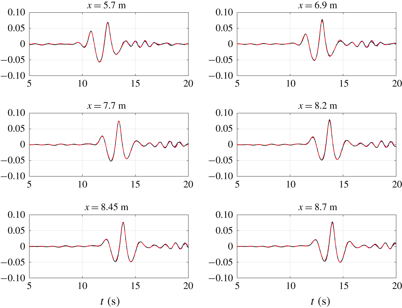
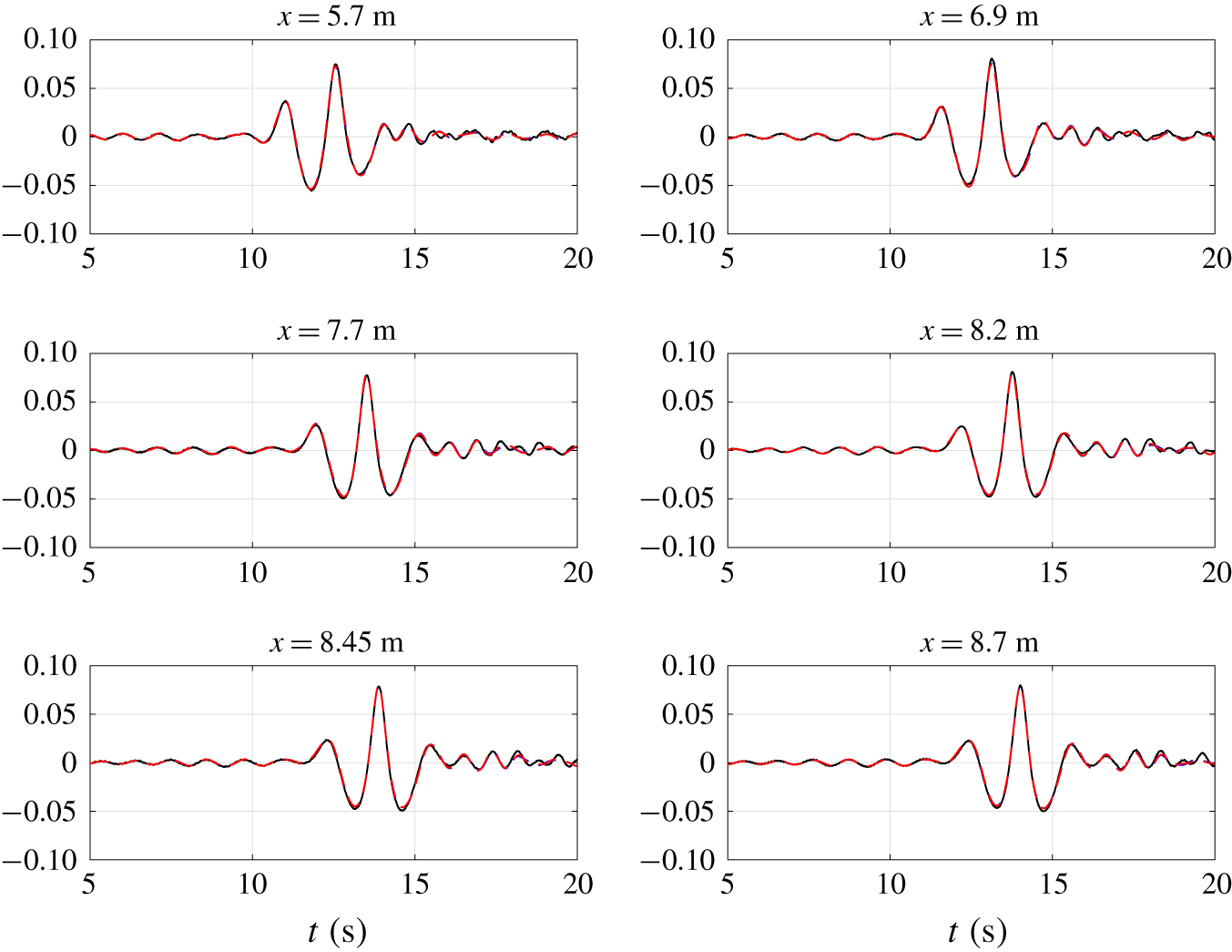
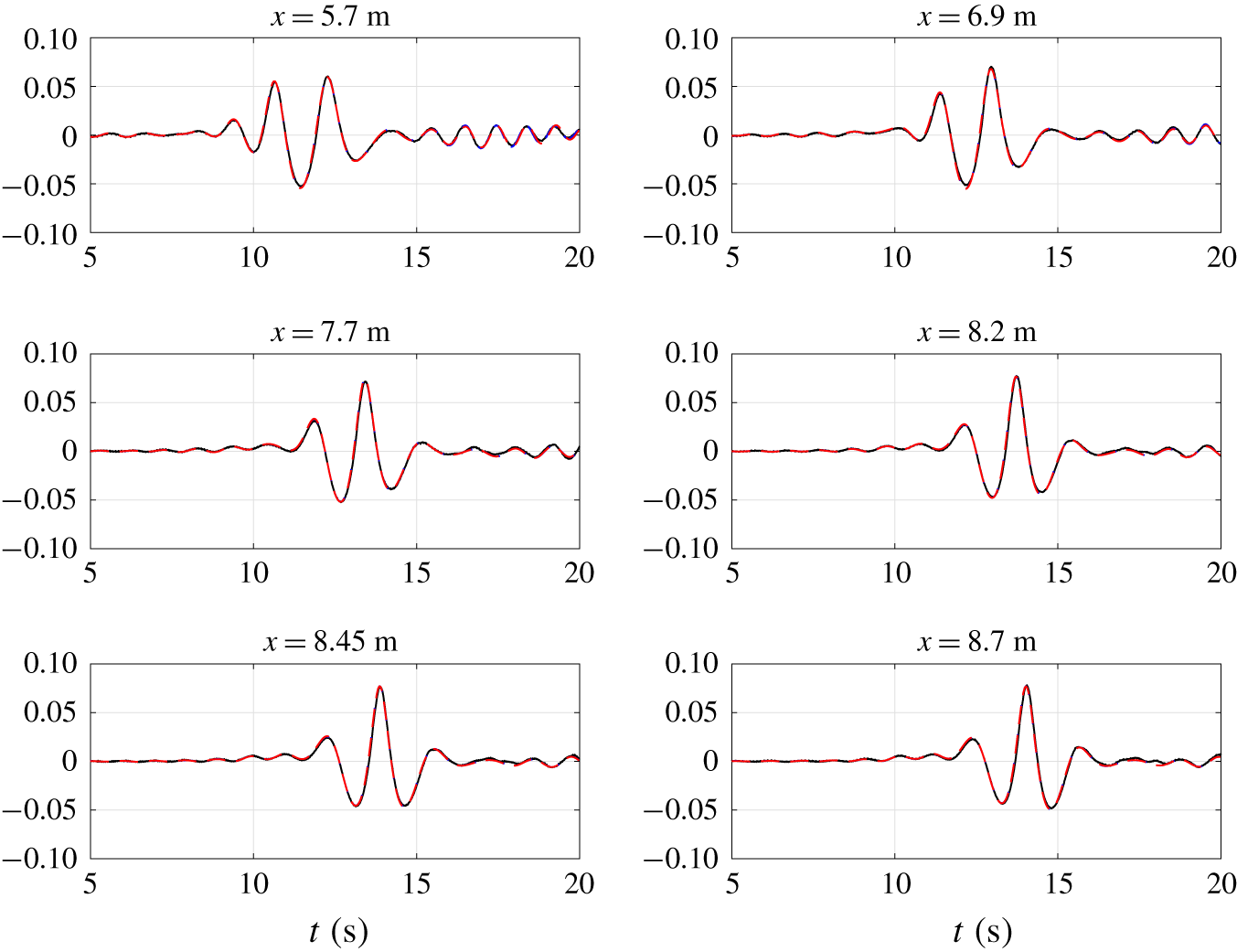
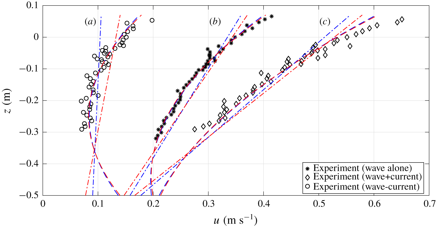
1 Introduction
Waves and currents are two dominating flow features in coastal water, engaging various physical processes with different spatial and temporal scales. As ocean waves propagate from deep water to shallow water they evolve through interaction with bathymetry and currents (e.g., reflection, refraction, diffraction and shoaling). Accurate descriptions of these phenomena are essential for understanding nearshore hydrodynamics and for engineering applications. For studying large scale (many wavelengths) wave propagation and scattering problems, two-dimensional horizontal (2DH) models are preferred over fully three-dimensional models for the huge difference in computational efficiency.
A number of 2DH depth-integrated models have been developed for nearshore applications over the past few decades. Based on the assumptions and approximations invoked, these models can be mainly classified as follows: weakly nonlinear and weakly dispersive (e.g., Boussinesq-type) models (Peregrine Reference Peregrine1967; Nwogu Reference Nwogu1993), fully nonlinear and weakly dispersive (e.g., extended Boussinesq-type) models (Liu Reference Liu and Liu1995; Wei et al. Reference Wei, Kirby, Grilli and Subramanya1995), multi-layer models (Lynett & Liu Reference Lynett and Liu2004a; Liu, Fang & Cheng Reference Liu, Fang and Cheng2018) and Green–Naghdi models (Green, Laws & Naghdi Reference Green, Laws and Naghdi1974; Shields & Webster Reference Shields and Webster1988; Webster, Duan & Zhao Reference Webster, Duan and Zhao2011). A brief review of these models is given below.
The weakly nonlinear and weakly dispersive (Boussinesq-type) models adopt two basic assumptions: (i) The flow either is irrotational or has weak horizontal vorticity components, and (ii) waves are in shallow water and wave amplitudes are small. For example, the classic Boussinesq wave model (Peregrine Reference Peregrine1967) requires that frequency dispersion and nonlinearity parameters are not only small, but also of the same order of magnitude, i.e.,  $O(\unicode[STIX]{x1D707}^{2})=O(\unicode[STIX]{x1D716})\ll 1$, where
 $\unicode[STIX]{x1D707}$ is the ratio between water depth and characteristic wavelength (
 $d/L$) and
 $\unicode[STIX]{x1D716}$ is the ratio between wave amplitude and water depth (
 $a/d$). The accuracy of the classic Boussinesq model is
 $O(\unicode[STIX]{x1D707}^{2})$. Therefore, the range of applicability of the classic Boussinesq model is limited to relatively shallow water (i.e.,
 $\unicode[STIX]{x1D707}<0.175$ or
 $kd<1.1$, where
 $k=2\unicode[STIX]{x03C0}/L$ is the characteristic wavenumber). Several efforts have been made to extend the applicable range of the classic Boussinesq model to intermediate and deep water by improving the linear frequency dispersion accuracy in ad hoc ways, while the nonlinearity is still kept small (e.g., Madsen & Sørensen Reference Madsen and Sørensen1991; Nwogu Reference Nwogu1993; Schäffer & Madsen Reference Schäffer and Madsen1995). It is well known that when waves approach the shore, nonlinearity becomes significant because of shoaling. To consider the nonlinear effects, a series of fully nonlinear and weakly dispersive wave (extended Boussinesq-type) models have been developed by treating the nonlinearity parameter
 $\unicode[STIX]{x1D716}$ as
 $O(1)$. Liu (Reference Liu and Liu1995) and Wei et al. (Reference Wei, Kirby, Grilli and Subramanya1995) developed similar models, which are still of
 $O(\unicode[STIX]{x1D707}^{2})$ accuracy. Gobbi, Kirby & Wei (Reference Gobbi, Kirby and Wei2000) included the
 $O(\unicode[STIX]{x1D707}^{4})$ terms in their model equations. Consequently, the linear wave frequency dispersion of the Gobbi et al. (Reference Gobbi, Kirby and Wei2000) model is accurate to the (4,4) Padé representation of the linear wave frequency dispersion relationship or
 $kd\approx 6$. However, the partial differential equations in the higher-order extended Boussinesq model contain higher spatial derivatives (
 ${>}3$), which require additional boundary conditions and also more computational effort.
Lynett & Liu (Reference Lynett and Liu2004a,Reference Lynett and Liub) offered an alternative approach in which they incorporated the multi-layer formulation with the fully nonlinear and weakly dispersive wave approximations. In their model, the water column is first divided into several layers with both the horizontal velocity and the pressure being matched at the interfaces between layers. A quadratic horizontal velocity profile and linear vertical velocity profile are employed by assuming weak  $(O(\unicode[STIX]{x1D707}^{4}))$ horizontal vorticity in each layer. More accurate velocity profiles in the water column and better representation of linear frequency dispersion relation can be obtained by increasing the number of layers. For example, the two-layer model exhibits accurate linear and nonlinear characteristics up to
 $kd\approx 6.5$. It is important to note that the highest spatial derivative in the multi-layer models is always the third. Moreover, for all the models discussed above, the water depth can vary significantly within a characteristic wavelength. Therefore, these models can simulate wave scattering, reflection, refraction, diffraction and shoaling.
More recently, Liu et al. (Reference Liu, Fang and Cheng2018) constructed a different type of multi-layer wave model for simulating highly dispersive and highly nonlinear waves over a slowly varying bottom. The model was developed specifically for potential flow and the governing equations were written in terms of the variables on the free surface (Agnon, Madsen & Schäffer Reference Agnon, Madsen and Schäffer1999). Following Lynett & Liu (Reference Lynett and Liu2004a), Liu et al. (Reference Liu, Fang and Cheng2018) also divided the water column into multiple layers. However, the long wave assumption was relaxed, and both horizontal velocity and vertical velocity were formulated using Taylor series expansions at a certain elevation. Thus, the vertical velocity must be solved explicitly instead of being expressed in terms of derivatives of horizontal velocity. Following Madsen, Bingham & Liu (Reference Madsen, Bingham and Liu2002) and Madsen, Bingham & Schäffer (Reference Madsen, Bingham and Schäffer2003), the linear and nonlinear properties were further enhanced and the resulting model demonstrated high accuracy in extremely deep water. For example, their two-layer model is accurate up to  $kd\approx 53$ with 1 % error in terms of linear frequency dispersion. However, we reiterate here that this model is restricted to potential flow and the water depth can only be slowly varying. Moreover, the multi-layer formulation inevitably requires solving more model equations. In the one-dimensional horizontal case, if
 $N$ layers are used,
 $(N+1)$ and
 $(2N+5)$ equations need to be solved for the models of Lynett & Liu (Reference Lynett and Liu2004a) and of Liu et al. (Reference Liu, Fang and Cheng2018), respectively.
Green et al. (Reference Green, Laws and Naghdi1974) and Green & Naghdi (Reference Green and Naghdi1976a,Reference Green and Naghdib) first derived the Green–Naghdi (GN) equations based on continuum mechanics theory and the concept of ‘directed fluid sheets’, which has its origin in the nonlinear plate and shell theory. Ertekin, Webster & Wehausen (Reference Ertekin, Webster and Wehausen1986) rederived the GN equations by assuming uniform horizontal velocity and linear vertical velocity profile in the water column, without using any small perturbation parameters and the irrotational flow assumption. This fully nonlinear GN model has been successfully applied to ship waves generated by a prescribed moving free surface pressure gradient. The GN equations (Ertekin et al. Reference Ertekin, Webster and Wehausen1986) can be shown to be the same as the model equations derived by Serre (Reference Serre1953), Su & Gardner (Reference Su and Gardner1969), and Barthélemy (Reference Barthélemy2004). Moreover, Lannes & Bonneton (Reference Lannes and Bonneton2009) verified that the GN equations (Green & Naghdi Reference Green and Naghdi1976a; Ertekin et al. Reference Ertekin, Webster and Wehausen1986) are equivalent to the fully nonlinear and weakly dispersive Boussinesq model (Wei et al. Reference Wei, Kirby, Grilli and Subramanya1995).
Another development of the GN equations is due to Shields & Webster (Reference Shields and Webster1988), who used the Kantorovich method (Kantorovich & Krylov Reference Kantorovich and Krylov1958) to reduce the dimensionality of a problem. Shields & Webster (Reference Shields and Webster1988) derived the GN equations for steady two-dimensional (horizontal and vertical) flows by assuming the horizontal velocity profile as a polynomial of the vertical coordinate up to the second degree. Demirbilek & Webster (Reference Demirbilek and Webster1992, Reference Demirbilek and Webster1999) derived the so-called level I and level II (level  $K$ corresponds to a
 $(K-1)$ degree horizontal velocity assumption in the present paper) GN equations and further applied these equations to some simple shallow water and nonlinear wave propagation problems. Extending the work of Demirbilek & Webster (Reference Demirbilek and Webster1999), Webster et al. (Reference Webster, Duan and Zhao2011) provided an improved derivation of the GN equations for higher polynomial approximations in the velocity profiles. In developing the above GN models, the velocity components are first approximated as a finite series of inner products of two sets of functions: a pre-selected shape or trial functions, depending only on the vertical coordinate, and unknown functions to be determined, depending on horizontal coordinates and time. Since these solutions are not exact, residuals can be calculated from the governing equations. The Galerkin method is then applied. Thus, the same set of shape functions is employed as the weighting functions in evaluating the residuals. In general, the resulting GN equations are very lengthy, which significantly influences the computational efficiency. Thus, practical applications and benchmark validations of GN models are still limited (Zhao, Duan & Ertekin Reference Zhao, Duan and Ertekin2014). Furthermore, to the best of our knowledge, only the linear frequency dispersion accuracy of the GN models has been analysed by Webster et al. (Reference Webster, Duan and Zhao2011). Theoretical analysis of other linear and nonlinear wave characteristics of the GN models is still in needed.
The wave frequency dispersion relation and internal kinematics of water waves can be strongly influenced by the presence of currents (Peregrine Reference Peregrine1976; Kirby & Chen Reference Kirby and Chen1989; Ellingsen & Li Reference Ellingsen and Li2017), and the vertical structure of the current can also be modified by wave motions (Thomas Reference Thomas1981, Reference Thomas1990; Kemp & Simons Reference Kemp and Simons1982, Reference Kemp and Simons1983; Swan, Cummins & James Reference Swan, Cummins and James2001). The complete coupling between waves and currents of various strengths and scales is still not well understood. Wave–current interactions based on the classic weakly nonlinear and weakly dispersive (Boussinesq-type) model have been investigated by Yoon & Liu (Reference Yoon and Liu1989), in which the current velocity is assumed to be stronger than the wave orbital velocity, but weaker than the phase velocity. The resulting model can only deal with nearly uniform current and is limited to wave–current interactions in relatively shallow water. On the other hand, other attempts have been made to include the influence of weakly sheared currents and bottom boundary layer effects in the Boussinesq-type wave models (Kim, Lynett & Socolofsky Reference Kim, Lynett and Socolofsky2009; Son & Lynett Reference Son and Lynett2014). Contributions from the second-order  $(O(\unicode[STIX]{x1D707}^{2}))$ horizontal vorticity are represented by an empirical model that describes both waves alone and wave–current induced bottom shear stress. More recently, Castro & Lannes (Reference Castro and Lannes2014) derived the fully nonlinear and weakly dispersive wave models in the presence of
 $O(\unicode[STIX]{x1D707})$ horizontal vorticity in shallow water. The depth-averaged horizontal vorticity effect is included by solving a finite number of cascade equations derived from the vorticity transport equation. In total, five coupled equations must be solved for the one-dimensional case. However, the restrictions of this model (Castro & Lannes Reference Castro and Lannes2014) are as follows: (i) the order of magnitude of the horizontal vorticity has to be small; (ii) the velocity field can be reconstructed only at the precision of the model; and (iii) these models can only be applied to relatively shallow water similar to classic Boussinesq-type wave models (Peregrine Reference Peregrine1967) because of their limited linear frequency dispersion accuracy.
A ‘coupled-mode model’ has recently been derived by Belibassakis & Touboul (Reference Belibassakis and Touboul2019). In their model the horizontal velocity is approximated as a finite series of trigonometric functions (eigenfunctions), which are orthogonal to each other. A pseudo-frequency must be selected for each problem to determine the eigenvalues associated with each mode in the solution series. Strictly speaking these eigenvalues depend on not only the water depth but also on the free surface elevation for nonlinear waves. Therefore, they need to be determined temporally and spatially. If the mild-slope and the small amplitude assumptions are invoked then these eigenvalues can be approximated as constants, which can obtained by solving a frequency dispersion relation equation with the selected pseudo-frequency and a reference water depth. Most of the model applications have been limited to such simplifications.
Non-hydrostatic models solve Reynolds-averaged Navier–Stokes equations with modified free surface boundary conditions, in which the free surface is restricted to being a single-valued function as in depth-integrated models. The non-hydrostatic models remain three-dimensional since they require solving the three-dimensional pressure Poisson equation (PPE). A theoretical analysis of linear and nonlinear properties of non-hydrostatic models has been conducted by Bai & Cheung (Reference Bai and Cheung2013), in which the non-hydrostatic models were put into depth-integrated forms. An accurate linear wave dispersion relation can be obtained by using just a few vertical layers. For example, a two-layer model is accurate up to  $kd\approx 8.8$ with only 2 % relative error in phase speed. However, it should be noted that in non-hydrostatic models the horizontal velocities are represented by ‘layer-averaged’ velocities, while vertical velocities are formulated in a piecewise-linear manner. Thus, although free-surface waves can be accurately predicted by using only a few vertical layers, the information about the underlying velocity field is rather limited. The computational cost will increase significantly by solving the PPE if more vertical layers employed.
Based on the brief literature review given above, it is clear that while Boussinesq-type models offer an efficient way towards calculating wave transformation from deep to shallow water, it is restricted to the weak horizontal vorticity assumption, making it unsuitable for simulating waves interacting with sheared currents. Although GN models provide an alternative approach to nearshore wave–current modelling, the procedures used in approximating the velocity and momentum equations result in pressure field information being missing, and the resulting model equations are generally lengthy and complex, which demand more computational effort. In this paper, using the concept of the method of weighted residuals, two sets of new models are derived (i.e., the Galerkin method model and the subdomain method model, respectively) so as to reduce two-dimensional (vertical and horizontal) problems into one-dimensional (horizontal) problems. These models are developed in the  $\unicode[STIX]{x1D70E}$-coordinate system, which transforms the total water depth in the physical domain onto a constant range of
 $\unicode[STIX]{x1D70E}$-coordinates. Although the new models based on the Galerkin method have the same mathematical basis as the GN models derived by Shields & Webster (Reference Shields and Webster1988), Demirbilek & Webster (Reference Demirbilek and Webster1999) and Webster et al. (Reference Webster, Duan and Zhao2011), the new models provide an explicit expression of the pressure field and exhibit simpler model equations, which is realized by using the
 $\unicode[STIX]{x1D70E}$-coordinate transformation together with orthogonal functions being employed as the shape functions. Therefore, the new Galerkin models require less computational time than the equivalent GN models. Lastly, the new models based on the subdomain method have superior wave properties and better computational efficiencies to the new models based on the Galerkin method, which also outperform the GN models.
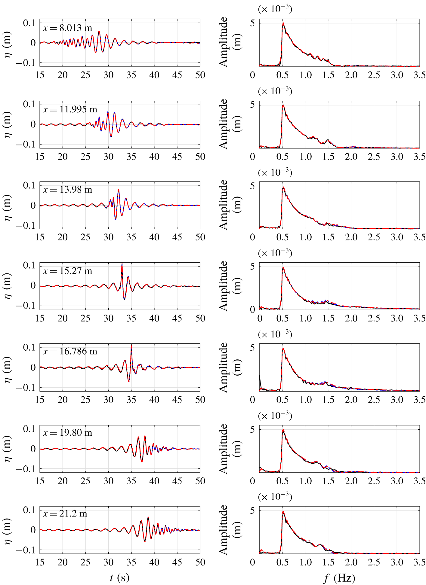
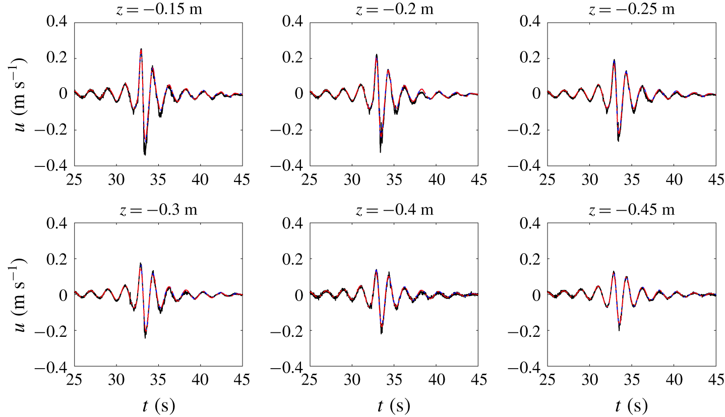
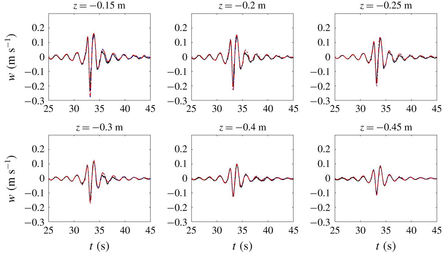
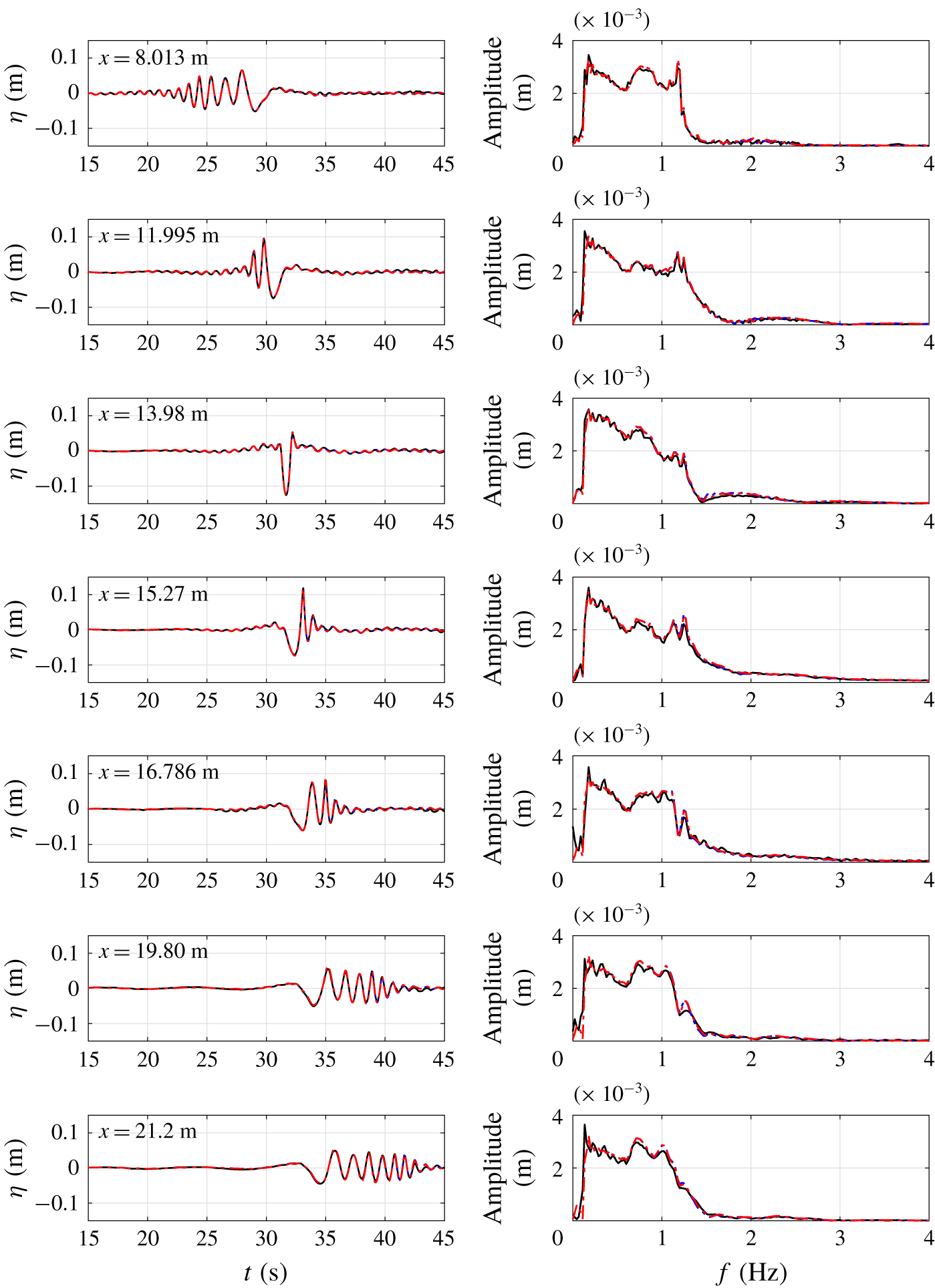
This paper is organized as follows: Section 2 describes the mathematical formulation of the new depth-integrated models. Theoretical analyses of the model performance in terms of linear and nonlinear water wave properties, as well as wave Doppler shift effects in the presence of currents, are conducted in § 3. We should point out that the derivations and analyses of the mathematical models are carried out by using the symbolic manipulation software, Mathematica™. The new mathematical models are implemented numerically and checked with several benchmark problems and newly conducted physical experiments, which are discussed in § 4. Finally, conclusions and future work are presented in § 5.
2 Derivation of mathematical models
In this section, a  $\unicode[STIX]{x1D70E}$-coordinate transformation is first introduced to map the water column bounded by a free surface and a deformable solid bottom to a specified constant interval. A general derivation of approximated horizontal momentum equations and the corresponding vertical velocity and pressure fields are followed. Finally, two new sets of one-dimensional mathematical models are obtained by applying the Galerkin method and the subdomain method on the horizontal momentum equations, respectively.
2.1 Governing equations
The present models are based on Euler’s equations with appropriate boundary conditions for incompressible and inviscid fluid. For clarity, only two-dimensional vertical plane problems are considered here. The extension of the present derivation to three-dimensional problems with two horizontal dimensions is straightforward but lengthy. The 2DH models will be presented in a future work with additional comparisons with three-dimensional benchmark problems. Thus, the governing equations and boundary conditions in Cartesian coordinates  $(x^{\ast },z^{\ast },t^{\ast })$ read
 $$\begin{eqnarray}\displaystyle & \displaystyle \frac{\unicode[STIX]{x2202}u}{\unicode[STIX]{x2202}x^{\ast }}+\frac{\unicode[STIX]{x2202}w}{\unicode[STIX]{x2202}z^{\ast }}=0, & \displaystyle\end{eqnarray}$$
 $$\begin{eqnarray}\displaystyle & \displaystyle \frac{\unicode[STIX]{x2202}u}{\unicode[STIX]{x2202}t^{\ast }}+u\frac{\unicode[STIX]{x2202}u}{\unicode[STIX]{x2202}x^{\ast }}+w\frac{\unicode[STIX]{x2202}u}{\unicode[STIX]{x2202}z^{\ast }}=-\frac{1}{\unicode[STIX]{x1D70C}}\frac{\unicode[STIX]{x2202}p}{\unicode[STIX]{x2202}x^{\ast }}, & \displaystyle\end{eqnarray}$$
 $$\begin{eqnarray}\displaystyle & \displaystyle \frac{\unicode[STIX]{x2202}w}{\unicode[STIX]{x2202}t^{\ast }}+u\frac{\unicode[STIX]{x2202}w}{\unicode[STIX]{x2202}x^{\ast }}+w\frac{\unicode[STIX]{x2202}w}{\unicode[STIX]{x2202}z^{\ast }}=-\frac{1}{\unicode[STIX]{x1D70C}}\frac{\unicode[STIX]{x2202}p}{\unicode[STIX]{x2202}z^{\ast }}-g; & \displaystyle\end{eqnarray}$$
 $$\begin{eqnarray}p=0,\quad z^{\ast }=\unicode[STIX]{x1D702}(x^{\ast },t^{\ast }),\end{eqnarray}$$
 $$\begin{eqnarray}\frac{\unicode[STIX]{x2202}\unicode[STIX]{x1D702}}{\unicode[STIX]{x2202}t^{\ast }}+u\frac{\unicode[STIX]{x2202}\unicode[STIX]{x1D702}}{\unicode[STIX]{x2202}x^{\ast }}=w,\quad z^{\ast }=\unicode[STIX]{x1D702}(x^{\ast },t^{\ast }),\end{eqnarray}$$
 $$\begin{eqnarray}\frac{\unicode[STIX]{x2202}h}{\unicode[STIX]{x2202}t^{\ast }}+u\frac{\unicode[STIX]{x2202}h}{\unicode[STIX]{x2202}x^{\ast }}+w=0,\quad z^{\ast }=-h(x^{\ast },t^{\ast }),\end{eqnarray}$$
where  $u$ and
 $w$ are the horizontal and vertical velocity, respectively, and
 $p$ is the pressure field. The total fluid domain is bounded by a deformable impermeable bottom,
 $z^{\ast }=-h(x^{\ast },t^{\ast })$, and the free surface,
 $z^{\ast }=\unicode[STIX]{x1D702}(x^{\ast },t^{\ast })$. Finally,
 $\unicode[STIX]{x1D70C}$ is the density of water and
 $g$ is the gravitational acceleration. Both of them are constants. The Euler equations consist of a continuity equation, (2.1), and horizontal and vertical momentum equations, (2.2) and (2.3), respectively. On the free surface, the dynamic and kinematic boundary conditions are specified in (2.4) and (2.5), respectively. Along the solid bottom, equation (2.6) represents the no-flux condition.
Equations (2.1)–(2.6) are written in Cartesian coordinates with the  $x^{\ast }$-axis being located at the still water level and the
 $z^{\ast }$-axis pointing upwards. The vorticity cannot be generated inside the flow domain since the fluid is inviscid and the flow is two-dimensional. However, the vorticity can still exist in the flow domain because of pre-existing conditions.
To facilitate the adoption of the method of weighted residuals in developing the present models, a  $\unicode[STIX]{x1D70E}$-coordinate transformation is performed to map the water column from
 $[-h,\unicode[STIX]{x1D702}]$ to a fixed range
 $[\unicode[STIX]{x1D6FC},\unicode[STIX]{x1D6FD}]$ in the
 $\unicode[STIX]{x1D70E}$-coordinate system. This transformation is defined as follows:
 $$\begin{eqnarray}t=t^{\ast },\quad x=x^{\ast },\quad \unicode[STIX]{x1D70E}=\unicode[STIX]{x1D70E}(z^{\ast },h(x^{\ast },t^{\ast }),\unicode[STIX]{x1D702}(x^{\ast },t^{\ast })),\end{eqnarray}$$
where  $\unicode[STIX]{x1D70E}$ is a function of free surface elevation and sea bottom configuration. Substituting (2.7) into (2.1)–(2.3) and using the chain rule, the governing equations in the
 $\unicode[STIX]{x1D70E}$-coordinate system are given as follows:
 $$\begin{eqnarray}\displaystyle & \displaystyle \frac{\unicode[STIX]{x2202}u}{\unicode[STIX]{x2202}x}+\frac{\unicode[STIX]{x2202}u}{\unicode[STIX]{x2202}\unicode[STIX]{x1D70E}}\frac{\unicode[STIX]{x2202}\unicode[STIX]{x1D70E}}{\unicode[STIX]{x2202}x^{\ast }}+\frac{\unicode[STIX]{x2202}w}{\unicode[STIX]{x2202}\unicode[STIX]{x1D70E}}\frac{\unicode[STIX]{x2202}\unicode[STIX]{x1D70E}}{\unicode[STIX]{x2202}z^{\ast }}=0, & \displaystyle\end{eqnarray}$$
 $$\begin{eqnarray}\displaystyle & \displaystyle \frac{\unicode[STIX]{x2202}u}{\unicode[STIX]{x2202}t}+\frac{\unicode[STIX]{x2202}u}{\unicode[STIX]{x2202}\unicode[STIX]{x1D70E}}\frac{\unicode[STIX]{x2202}\unicode[STIX]{x1D70E}}{\unicode[STIX]{x2202}t^{\ast }}+u\left(\frac{\unicode[STIX]{x2202}u}{\unicode[STIX]{x2202}x}+\frac{\unicode[STIX]{x2202}u}{\unicode[STIX]{x2202}\unicode[STIX]{x1D70E}}\frac{\unicode[STIX]{x2202}\unicode[STIX]{x1D70E}}{\unicode[STIX]{x2202}x^{\ast }}\right)+w\frac{\unicode[STIX]{x2202}u}{\unicode[STIX]{x2202}\unicode[STIX]{x1D70E}}\frac{\unicode[STIX]{x2202}\unicode[STIX]{x1D70E}}{\unicode[STIX]{x2202}z^{\ast }}=-\frac{1}{\unicode[STIX]{x1D70C}}\left(\frac{\unicode[STIX]{x2202}p}{\unicode[STIX]{x2202}x}+\frac{\unicode[STIX]{x2202}p}{\unicode[STIX]{x2202}\unicode[STIX]{x1D70E}}\frac{\unicode[STIX]{x2202}\unicode[STIX]{x1D70E}}{\unicode[STIX]{x2202}x^{\ast }}\right), & \displaystyle\end{eqnarray}$$
 $$\begin{eqnarray}\displaystyle & \displaystyle \frac{\unicode[STIX]{x2202}w}{\unicode[STIX]{x2202}t}+\frac{\unicode[STIX]{x2202}w}{\unicode[STIX]{x2202}\unicode[STIX]{x1D70E}}\frac{\unicode[STIX]{x2202}\unicode[STIX]{x1D70E}}{\unicode[STIX]{x2202}t^{\ast }}+u\left(\frac{\unicode[STIX]{x2202}w}{\unicode[STIX]{x2202}x}+\frac{\unicode[STIX]{x2202}w}{\unicode[STIX]{x2202}\unicode[STIX]{x1D70E}}\frac{\unicode[STIX]{x2202}\unicode[STIX]{x1D70E}}{\unicode[STIX]{x2202}x^{\ast }}\right)+w\frac{\unicode[STIX]{x2202}w}{\unicode[STIX]{x2202}\unicode[STIX]{x1D70E}}\frac{\unicode[STIX]{x2202}\unicode[STIX]{x1D70E}}{\unicode[STIX]{x2202}z^{\ast }}=-\frac{1}{\unicode[STIX]{x1D70C}}\frac{\unicode[STIX]{x2202}p}{\unicode[STIX]{x2202}\unicode[STIX]{x1D70E}}\frac{\unicode[STIX]{x2202}\unicode[STIX]{x1D70E}}{\unicode[STIX]{x2202}z^{\ast }}-g. & \displaystyle\end{eqnarray}$$
The boundary conditions in the new coordinate system are,
 $$\begin{eqnarray}p_{s}=0,\quad \unicode[STIX]{x1D70E}=\unicode[STIX]{x1D6FD},\end{eqnarray}$$
 $$\begin{eqnarray}\frac{\unicode[STIX]{x2202}\unicode[STIX]{x1D702}}{\unicode[STIX]{x2202}t}+u_{s}\frac{\unicode[STIX]{x2202}\unicode[STIX]{x1D702}}{\unicode[STIX]{x2202}x}=w_{s},\quad \unicode[STIX]{x1D70E}=\unicode[STIX]{x1D6FD},\end{eqnarray}$$
 $$\begin{eqnarray}\frac{\unicode[STIX]{x2202}h}{\unicode[STIX]{x2202}t}+u_{b}\frac{\unicode[STIX]{x2202}h}{\unicode[STIX]{x2202}x}+w_{b}=0,\quad \unicode[STIX]{x1D70E}=\unicode[STIX]{x1D6FC},\end{eqnarray}$$
where the subscripts  $s$ and
 $b$ indicate that the physical variables are evaluated at the free surface and the sea bottom, respectively.
By vertically integrating the continuity equation (2.1) from  $z^{\ast }=-h$ to
 $\unicode[STIX]{x1D702}$ and applying the boundary conditions, equations (2.5) and (2.6), we obtain the well known depth-integrated continuity equation
 $$\begin{eqnarray}\frac{\unicode[STIX]{x2202}H}{\unicode[STIX]{x2202}t^{\ast }}+\frac{\unicode[STIX]{x2202}}{\unicode[STIX]{x2202}x^{\ast }}\int _{-h}^{\unicode[STIX]{x1D702}}u\,\text{d}z^{\ast }=0,\end{eqnarray}$$
where  $H$ is the total water depth, being defined as
 $H=\unicode[STIX]{x1D702}+h$. Note that the above equation is exact and represents the mass conservation, integrated over water column. Equation (2.14) can be directly transformed into
 $\unicode[STIX]{x1D70E}$-coordinates as follows:
 $$\begin{eqnarray}\frac{\unicode[STIX]{x2202}H}{\unicode[STIX]{x2202}t}+\frac{\unicode[STIX]{x2202}}{\unicode[STIX]{x2202}x}\left(\int _{\unicode[STIX]{x1D6FC}}^{\unicode[STIX]{x1D6FD}}\frac{1}{\left({\displaystyle \frac{\unicode[STIX]{x2202}\unicode[STIX]{x1D70E}}{\unicode[STIX]{x2202}z^{\ast }}}\right)}u\,\text{d}\unicode[STIX]{x1D70E}\right)=0.\end{eqnarray}$$
2.2 Method of weighted residuals
Following the method of weighted residuals (Finlayson Reference Finlayson2013), a trial solution  $\tilde{u}$ is expressed as an infinite series of products of a function,
 $u_{i}(x,t)$, depending on the horizontal coordinate
 $x$ and time
 $t$, and another function,
 $N_{i}(\unicode[STIX]{x1D70E})$, with only vertical (
 $\unicode[STIX]{x1D70E}$) dependence, i.e.,
 $$\begin{eqnarray}\tilde{u} (x,\unicode[STIX]{x1D70E},t)=\mathop{\sum }_{i=0}^{K-1}u_{i}(x,t)N_{i}(\unicode[STIX]{x1D70E}),\end{eqnarray}$$
where the infinite series has been truncated to  $K$ terms. While the
 $N_{i}$ functions determine the vertical structure of the horizontal velocity and are often called trial functions or shape functions,
 $u_{i}$ are a set of functions to be determined from the resulting model. The trial functions
 $N_{i}$ must be complete and linearly independent. The completeness property ensures that the exact solution can be represented by a set of trial functions provided that enough terms are used (Finlayson Reference Finlayson2013).
Once the vertical structure of the horizontal velocity is specified, the vertical velocity can be derived by vertically integrating the continuity equation, (2.8), from the bottom, ( $\unicode[STIX]{x1D70E}=\unicode[STIX]{x1D6FC}$), to an arbitrary
 $\unicode[STIX]{x1D70E}$ value in the water column and applying the kinematic boundary condition at the bottom, (2.13). Thus, the expression for the vertical velocity is obtained as
 $$\begin{eqnarray}\tilde{w}=-\frac{\unicode[STIX]{x2202}h}{\unicode[STIX]{x2202}t}-u_{b}\frac{\unicode[STIX]{x2202}h}{\unicode[STIX]{x2202}x}-\frac{1}{\left({\displaystyle \frac{\unicode[STIX]{x2202}\unicode[STIX]{x1D70E}}{\unicode[STIX]{x2202}z^{\ast }}}\right)}\left[\int _{\unicode[STIX]{x1D6FC}}^{\unicode[STIX]{x1D70E}}\left(\frac{\unicode[STIX]{x2202}\tilde{u} }{\unicode[STIX]{x2202}x}+\frac{\unicode[STIX]{x2202}\tilde{u} }{\unicode[STIX]{x2202}\unicode[STIX]{x1D70E}}\frac{\unicode[STIX]{x2202}\unicode[STIX]{x1D70E}}{\unicode[STIX]{x2202}x^{\ast }}\right)\,\text{d}\unicode[STIX]{x1D70E}\right].\end{eqnarray}$$
Substituting the trial horizontal velocity, (2.16), into the equation above, the corresponding trial vertical velocity can be expressed as a function of  $u_{i}$ and their derivatives.
We remark here that in the development of GN model the trial solutions for the horizontal velocity components and the vertical velocity component were independently expressed in the same series form as (2.16) in Cartesian coordinates. This led to additional weighted horizontal momentum equations that were redundant for constructing the final equations system, and were simply discarded. Moreover, in deriving GN models a certain ad hoc simplification, such as the so-called ‘restricted theory’, must be imposed (see Demirbilek & Webster Reference Demirbilek and Webster1992; Webster et al. Reference Webster, Duan and Zhao2011).
The pressure field is derived by vertically integrating the vertical momentum equation, (2.10), from an arbitrary  $\unicode[STIX]{x1D70E}$ level to the free surface (
 $\unicode[STIX]{x1D70E}=\unicode[STIX]{x1D6FD}$) and applying the dynamic boundary condition (2.11). Thus,
 $$\begin{eqnarray}\tilde{p}=\frac{1}{\left({\displaystyle \frac{\unicode[STIX]{x2202}\unicode[STIX]{x1D70E}}{\unicode[STIX]{x2202}z^{\ast }}}\right)}\left[\unicode[STIX]{x1D70C}g(\unicode[STIX]{x1D6FD}-\unicode[STIX]{x1D70E})\!+\unicode[STIX]{x1D70C}\int _{\unicode[STIX]{x1D70E}}^{\unicode[STIX]{x1D6FD}}\!\left(\frac{\unicode[STIX]{x2202}\tilde{w}}{\unicode[STIX]{x2202}t}+\frac{\unicode[STIX]{x2202}\tilde{w}}{\unicode[STIX]{x2202}\unicode[STIX]{x1D70E}}\frac{\unicode[STIX]{x2202}\unicode[STIX]{x1D70E}}{\unicode[STIX]{x2202}t^{\ast }}+\tilde{u} \left(\frac{\unicode[STIX]{x2202}\tilde{w}}{\unicode[STIX]{x2202}x}+\frac{\unicode[STIX]{x2202}\tilde{w}}{\unicode[STIX]{x2202}\unicode[STIX]{x1D70E}}\frac{\unicode[STIX]{x2202}\unicode[STIX]{x1D70E}}{\unicode[STIX]{x2202}x^{\ast }}\right)\!+\tilde{w}\frac{\unicode[STIX]{x2202}\tilde{w}}{\unicode[STIX]{x2202}\unicode[STIX]{x1D70E}}\frac{\unicode[STIX]{x2202}\unicode[STIX]{x1D70E}}{\unicode[STIX]{x2202}z^{\ast }}\right)\text{d}\unicode[STIX]{x1D70E}\right],\end{eqnarray}$$
where the first term represents the hydrostatic pressure and the second term is the non-hydrostatic correction. Substituting the trial solutions for horizontal velocity, (2.16), and trial vertical velocity, (2.17), into the equation above, the trial solution for pressure field can also be expressed in terms of  $u_{i}$ and their various derivatives. Thus once
 $u_{i}$ are determined, the trial velocity and pressure fields are also described.
To find the solutions for  $u_{i}$, the trial solutions of the velocity and pressure fields, (2.16) to (2.18), are substituted into the horizontal momentum equation, (2.2). This operation produces a residual function,
 $R$, since the trial functions are not the exact solutions of the momentum equation. Thus,
 $$\begin{eqnarray}R=\frac{\unicode[STIX]{x2202}\tilde{u} }{\unicode[STIX]{x2202}t}+\frac{\unicode[STIX]{x2202}\tilde{u} }{\unicode[STIX]{x2202}\unicode[STIX]{x1D70E}}\frac{\unicode[STIX]{x2202}\unicode[STIX]{x1D70E}}{\unicode[STIX]{x2202}t^{\ast }}+\tilde{u} \left(\frac{\unicode[STIX]{x2202}\tilde{u} }{\unicode[STIX]{x2202}x}+\frac{\unicode[STIX]{x2202}\tilde{u} }{\unicode[STIX]{x2202}\unicode[STIX]{x1D70E}}\frac{\unicode[STIX]{x2202}\unicode[STIX]{x1D70E}}{\unicode[STIX]{x2202}x^{\ast }}\right)+\tilde{w}\frac{\unicode[STIX]{x2202}\tilde{u} }{\unicode[STIX]{x2202}\unicode[STIX]{x1D70E}}\frac{\unicode[STIX]{x2202}\unicode[STIX]{x1D70E}}{\unicode[STIX]{x2202}z^{\ast }}+\frac{1}{\unicode[STIX]{x1D70C}}\left(\frac{\unicode[STIX]{x2202}\tilde{p}}{\unicode[STIX]{x2202}x}+\frac{\unicode[STIX]{x2202}\tilde{p}}{\unicode[STIX]{x2202}\unicode[STIX]{x1D70E}}\frac{\unicode[STIX]{x2202}\unicode[STIX]{x1D70E}}{\unicode[STIX]{x2202}x^{\ast }}\right).\end{eqnarray}$$
We reiterate here that the residual  $R$ can be expressed in terms of
 $u_{i}$ and their derivatives.
Following the method of weighted residuals, the unknown functions  $u_{i}$ are determined in such a way that the weighted residual is forced to be zero in the globally integrated sense (Finlayson Reference Finlayson2013, p. 20). Thus,
 $K$ weighting functions need to be selected and the weighted residuals integrated over the water column are forced to be zero,
 $$\begin{eqnarray}\int _{\unicode[STIX]{x1D6FC}}^{\unicode[STIX]{x1D6FD}}W_{j}R\,\text{d}\unicode[STIX]{x1D70E}=0,\quad j=1,2,\ldots ,K.\end{eqnarray}$$
The equation above represents a system of  $K$ nonlinear partial differential equations for
 $K$ horizontal velocity coefficients (
 $u_{0},u_{1},\ldots ,u_{K-1}$) and the total water depth,
 $H=\unicode[STIX]{x1D702}+h$. The additional governing equation comes from the depth-integrated continuity equation, (2.15).
We reiterate that in deriving GN models, the vertical momentum equation was treated in the same way as the horizontal momentum equation(s), which was(were) approximated in an averaged sense (depth-integrated) over the entire water column. Thus, the pressure related information was represented by depth-averaged quantities (e.g., depth-averaged pressure) in GN models, and no explicit expressions of the pressure field were available. On the other hand, in the present model, (2.18) provides such information, which is important in calculating wave forces.
The remaining question is how to choose the appropriate weighting functions. Several options are available, including the collocation method (Lanczos Reference Lanczos1938), the subdomain method (Biezeno Reference Biezeno1924), the Galerkin method (Galerkin Reference Galerkin1915), the least square method (Picone Reference Picone1928) and the moment method (Levich & Krylov Reference Levich and Krylov1969). In this paper, we employ the Galerkin method and the subdomain method for their accuracy and ease of formulation in deriving two sets of model equations.
2.3 Models based on the Galerkin method
The Galerkin method (Galerkin Reference Galerkin1915) uses the trial functions ( $N_{i}$) as weighting functions (
 $W_{i}$). We reiterate here that the trial functions must satisfy the completeness and linear-independence requirements. Since a continuous function must be zero if it is orthogonal to all members of a complete set of functions, the Galerkin method forces the residual function to be zero by making it orthogonal to the trial functions.
According to Weierstrass’s first theorem (Bellman & Roth Reference Bellman and Roth1986), any continuous function defined in  $[a,b]$ can be uniformly approximated by polynomials. Thus, general polynomials in the form of
 $N_{i}(\unicode[STIX]{x1D70E})=\sum _{j=1}^{i}a_{ij}\unicode[STIX]{x1D70E}^{j-1}$ are chosen here. It is noted that the free coefficients,
 $a_{ij}$, have no influence on the degree of polynomial approximation since the trial functions are linear combinations of the function space
 $\{1,\unicode[STIX]{x1D70E},\unicode[STIX]{x1D70E}^{2},\ldots \}$. Having said so, orthogonal functions (e.g., Legendre or Chebyshev type I functions) are preferred choices since the property of orthogonality significantly simplifies the resulting models. Furthermore, in the standard Galerkin method, Babuska, Práger & Vitásek (Reference Babuska, Práger and Vitásek1966) has suggested that orthogonal polynomials should be used for higher degree of polynomial approximations, otherwise, the computations could become unstable.
In this paper, Legendre functions are employed for a detailed analysis. Legendre functions satisfy the following recurrence relation (Abramowitz & Stegun Reference Abramowitz and Stegun1965)
 $$\begin{eqnarray}N_{i+1}(\unicode[STIX]{x1D70E})=\frac{2i+1}{i+1}\unicode[STIX]{x1D70E}N_{i}(\unicode[STIX]{x1D70E})-\frac{i}{i+1}N_{i-1}(\unicode[STIX]{x1D70E}),\end{eqnarray}$$
with the first four functions being
 $$\begin{eqnarray}N_{0}(\unicode[STIX]{x1D70E})=1,\quad N_{1}(\unicode[STIX]{x1D70E})=\unicode[STIX]{x1D70E},\quad N_{2}(\unicode[STIX]{x1D70E})={\textstyle \frac{1}{2}}(3\unicode[STIX]{x1D70E}^{2}-1),\quad N_{3}(\unicode[STIX]{x1D70E})={\textstyle \frac{1}{2}}(5\unicode[STIX]{x1D70E}^{3}-3\unicode[STIX]{x1D70E}).\end{eqnarray}$$
The orthogonality provides the following relation
 $$\begin{eqnarray}\int _{-1}^{1}N_{n}(\unicode[STIX]{x1D70E})N_{m}(\unicode[STIX]{x1D70E})\,\text{d}\unicode[STIX]{x1D70E}=\frac{2}{2n+1}\unicode[STIX]{x1D6FF}_{nm},\end{eqnarray}$$
where  $\unicode[STIX]{x1D6FF}_{nm}$ is the Kronecker delta.
Since the Legendre functions are orthogonal in  $[-1,1]$, in the following derivation an explicit
 $\unicode[STIX]{x1D70E}$-coordinate transformation in the vertical direction is defined so that
 $\unicode[STIX]{x1D70E}$ spans from
 $-1$ to
 $1$ (i.e.,
 $\unicode[STIX]{x1D6FC}=-1$ and
 $\unicode[STIX]{x1D6FD}=1$), which reads
 $$\begin{eqnarray}\unicode[STIX]{x1D70E}=\frac{2z^{\ast }+h-\unicode[STIX]{x1D702}}{h+\unicode[STIX]{x1D702}}=\frac{2z^{\ast }+2h-H}{H}.\end{eqnarray}$$
The expressions of its derivatives are given as follows:
 $$\begin{eqnarray}\frac{\unicode[STIX]{x2202}\unicode[STIX]{x1D70E}}{\unicode[STIX]{x2202}t^{\ast }}=\frac{1}{H}\left(2\frac{\unicode[STIX]{x2202}h}{\unicode[STIX]{x2202}t}-\frac{\unicode[STIX]{x2202}H}{\unicode[STIX]{x2202}t}-\unicode[STIX]{x1D70E}\frac{\unicode[STIX]{x2202}H}{\unicode[STIX]{x2202}t}\right),\quad \frac{\unicode[STIX]{x2202}\unicode[STIX]{x1D70E}}{\unicode[STIX]{x2202}x^{\ast }}=\frac{1}{H}\left(2\frac{\unicode[STIX]{x2202}h}{\unicode[STIX]{x2202}x}-\frac{\unicode[STIX]{x2202}H}{\unicode[STIX]{x2202}x}-\unicode[STIX]{x1D70E}\frac{\unicode[STIX]{x2202}H}{\unicode[STIX]{x2202}x}\right),\quad \frac{\unicode[STIX]{x2202}\unicode[STIX]{x1D70E}}{\unicode[STIX]{x2202}z^{\ast }}=\frac{2}{H}.\end{eqnarray}$$
Using Mathematica™, we have developed model equations for different values of  $K$ in (2.16), which corresponds to a polynomial of degree
 $(K-1)$ in
 $\unicode[STIX]{x1D70E}$. For the purpose of illustration, we provide the detailed derivation for
 $K=2$. Thus, the horizontal velocity is assumed to be linear in the vertical direction. The trial solution of horizontal velocity,
 $\tilde{u}$, based on Legendre functions (
 $K=2$) reads
 $$\begin{eqnarray}\displaystyle & \displaystyle N_{0}=1, & \displaystyle\end{eqnarray}$$
 $$\begin{eqnarray}\displaystyle & \displaystyle N_{1}=\unicode[STIX]{x1D70E}, & \displaystyle\end{eqnarray}$$
 $$\begin{eqnarray}\displaystyle & \displaystyle \tilde{u} (x,\unicode[STIX]{x1D70E},t)=u_{0}(x,t)+\unicode[STIX]{x1D70E}u_{1}(x,t). & \displaystyle\end{eqnarray}$$
The free surface evolution equation can be obtained by substituting the above equation into the depth-averaged continuity equation (2.15),
 $$\begin{eqnarray}\displaystyle \frac{\unicode[STIX]{x2202}H}{\unicode[STIX]{x2202}t}+\frac{\unicode[STIX]{x2202}(Hu_{0})}{\unicode[STIX]{x2202}x}=0. & & \displaystyle\end{eqnarray}$$
This equation remains the same for all models with higher degree of polynomial approximation ( $K>2$) because of the orthogonal property of the Legendre functions.
Substituting (2.28) into (2.17), the vertical velocity yields the following explicit expression:
 $$\begin{eqnarray}\displaystyle \tilde{w} & = & \displaystyle \frac{1}{4}\left(-4\frac{\unicode[STIX]{x2202}h}{\unicode[STIX]{x2202}x}u_{0}-4\frac{\unicode[STIX]{x2202}h}{\unicode[STIX]{x2202}t}+\frac{\unicode[STIX]{x2202}H}{\unicode[STIX]{x2202}x}u_{1}-2H\frac{\unicode[STIX]{x2202}u_{0}}{\unicode[STIX]{x2202}x}+H\frac{\unicode[STIX]{x2202}u_{1}}{\unicode[STIX]{x2202}x}\right)\nonumber\\ \displaystyle & & \displaystyle +\,\frac{1}{2}\unicode[STIX]{x1D70E}\left[u_{1}\left(\frac{\unicode[STIX]{x2202}H}{\unicode[STIX]{x2202}x}-2\frac{\unicode[STIX]{x2202}h}{\unicode[STIX]{x2202}x}\right)-H\frac{\unicode[STIX]{x2202}u_{0}}{\unicode[STIX]{x2202}x}\right]\nonumber\\ \displaystyle & & \displaystyle +\,\frac{1}{4}\unicode[STIX]{x1D70E}^{2}\left(\frac{\unicode[STIX]{x2202}H}{\unicode[STIX]{x2202}x}u_{1}-H\frac{\unicode[STIX]{x2202}u_{1}}{\unicode[STIX]{x2202}x}\right),\end{eqnarray}$$
which is a quadratic function in the vertical coordinate. In terms of the vorticity field, it is obvious that the vertical structure of the resulting horizontal vorticity field is also a quadratic polynomial,
 $$\begin{eqnarray}\displaystyle \unicode[STIX]{x1D714}_{h} & = & \displaystyle \frac{\unicode[STIX]{x2202}u}{\unicode[STIX]{x2202}z^{\ast }}-\frac{\unicode[STIX]{x2202}w}{\unicode[STIX]{x2202}x^{\ast }}\nonumber\\ \displaystyle & = & \displaystyle \frac{1}{4}\left[2\frac{u_{1}}{H}\left(-4\frac{\unicode[STIX]{x2202}h}{\unicode[STIX]{x2202}x}\frac{\unicode[STIX]{x2202}H}{\unicode[STIX]{x2202}x}+4\left(\frac{\unicode[STIX]{x2202}h}{\unicode[STIX]{x2202}x}\right)^{2}+\left(\frac{\unicode[STIX]{x2202}H}{\unicode[STIX]{x2202}x}\right)^{2}+4\right)+8\frac{\unicode[STIX]{x2202}h}{\unicode[STIX]{x2202}x}\frac{\unicode[STIX]{x2202}u_{0}}{\unicode[STIX]{x2202}x}+4\frac{\unicode[STIX]{x2202}^{2}h}{\unicode[STIX]{x2202}x^{2}}u_{0}\right.\nonumber\\ \displaystyle & & \displaystyle +\,\left.4\frac{\unicode[STIX]{x2202}^{2}h}{\unicode[STIX]{x2202}x\unicode[STIX]{x2202}t}-2\frac{\unicode[STIX]{x2202}H}{\unicode[STIX]{x2202}x}\frac{\unicode[STIX]{x2202}u_{1}}{\unicode[STIX]{x2202}x}-\frac{\unicode[STIX]{x2202}^{2}H}{\unicode[STIX]{x2202}x^{2}}u_{1}+H\left(2\frac{\unicode[STIX]{x2202}^{2}u_{0}}{\unicode[STIX]{x2202}x^{2}}-\frac{\unicode[STIX]{x2202}^{2}u_{1}}{\unicode[STIX]{x2202}x^{2}}\right)\right]\nonumber\\ \displaystyle & & \displaystyle +\left(\frac{1}{H}\frac{\unicode[STIX]{x2202}H}{\unicode[STIX]{x2202}x}u_{1}\left(\frac{\unicode[STIX]{x2202}H}{\unicode[STIX]{x2202}x}-2\frac{\unicode[STIX]{x2202}h}{\unicode[STIX]{x2202}x}\right)+2\frac{\unicode[STIX]{x2202}h}{\unicode[STIX]{x2202}x}\frac{\unicode[STIX]{x2202}u_{1}}{\unicode[STIX]{x2202}x}+\frac{\unicode[STIX]{x2202}^{2}h}{\unicode[STIX]{x2202}x^{2}}u_{1}\right.\nonumber\\ \displaystyle & & \displaystyle -\,\left.\frac{\unicode[STIX]{x2202}H}{\unicode[STIX]{x2202}x}\frac{\unicode[STIX]{x2202}u_{1}}{\unicode[STIX]{x2202}x}-\frac{1}{2}\frac{\unicode[STIX]{x2202}^{2}H}{\unicode[STIX]{x2202}x^{2}}u_{1}+\frac{1}{2}H\frac{\unicode[STIX]{x2202}^{2}u_{0}}{\unicode[STIX]{x2202}x^{2}}\right)\unicode[STIX]{x1D70E}\nonumber\\ \displaystyle & & \displaystyle +\,\frac{1}{4}\left(-2\frac{\unicode[STIX]{x2202}H}{\unicode[STIX]{x2202}x}\frac{\unicode[STIX]{x2202}u_{1}}{\unicode[STIX]{x2202}x}+\frac{1}{H}2\left(\frac{\unicode[STIX]{x2202}H}{\unicode[STIX]{x2202}x}\right)^{2}u_{1}-\frac{\unicode[STIX]{x2202}^{2}H}{\unicode[STIX]{x2202}x^{2}}u_{1}+H\frac{\unicode[STIX]{x2202}^{2}u_{1}}{\unicode[STIX]{x2202}x^{2}}\right)\unicode[STIX]{x1D70E}^{2}.\end{eqnarray}$$
Thus, a direct restriction on the horizontal vorticity field for the new models is the complexity of their vertical structure.
The pressure can be obtained by substituting the horizontal and vertical velocity expressions, (2.28) and (2.30), into the vertical momentum equation, (2.18), as
 $$\begin{eqnarray}\displaystyle \tilde{p}=\frac{(1-\unicode[STIX]{x1D70E})}{2}\unicode[STIX]{x1D70C}gH+\tilde{p}_{nh}. & & \displaystyle\end{eqnarray}$$
The non-hydrostatic pressure,  $\tilde{p}_{nh}$, is a fourth-degree polynomial in
 $\unicode[STIX]{x1D70E}$ with coefficients being functions of horizontal velocity variables and their horizontal derivatives, which can be found in § A of the supplementary materials (available athttps://doi.org/10.1017/jfm.2019.831).
In summary, for the  $K=2$ model, there are three unknown functions,
 $u_{0}$,
 $u_{1}$ and the total depth,
 $H$. All of them are functions of horizontal coordinate,
 $x$, and time,
 $t$. Once these unknown functions are found, the velocity field, (2.28) and (2.30), and the pressure field, (2.32), are determined. To obtain the model equations for these unknown functions, we apply the Galerkin method. Thus, by choosing the weighting functions to be the same as the trial functions, namely,
 $W_{i}=N_{i}$, (2.20) yields two equivalent momentum equations for
 $K=2$. Thus
 $$\begin{eqnarray}\displaystyle & & \displaystyle \int _{-1}^{1}N_{0}\left[\frac{\unicode[STIX]{x2202}\tilde{u} }{\unicode[STIX]{x2202}t}+\frac{\unicode[STIX]{x2202}\tilde{u} }{\unicode[STIX]{x2202}\unicode[STIX]{x1D70E}}\frac{\unicode[STIX]{x2202}\unicode[STIX]{x1D70E}}{\unicode[STIX]{x2202}t^{\ast }}+\tilde{u} \left(\frac{\unicode[STIX]{x2202}\tilde{u} }{\unicode[STIX]{x2202}x}+\frac{\unicode[STIX]{x2202}\tilde{u} }{\unicode[STIX]{x2202}\unicode[STIX]{x1D70E}}\frac{\unicode[STIX]{x2202}\unicode[STIX]{x1D70E}}{\unicode[STIX]{x2202}x^{\ast }}\right)\right.\nonumber\\ \displaystyle & & \displaystyle \qquad \left.+\,\tilde{w}\frac{\unicode[STIX]{x2202}\tilde{u} }{\unicode[STIX]{x2202}\unicode[STIX]{x1D70E}}\frac{\unicode[STIX]{x2202}\unicode[STIX]{x1D70E}}{\unicode[STIX]{x2202}z^{\ast }}+\frac{1}{\unicode[STIX]{x1D70C}}\left(\frac{\unicode[STIX]{x2202}\tilde{p}}{\unicode[STIX]{x2202}x}+\frac{\unicode[STIX]{x2202}\tilde{p}}{\unicode[STIX]{x2202}\unicode[STIX]{x1D70E}}\frac{\unicode[STIX]{x2202}\unicode[STIX]{x1D70E}}{\unicode[STIX]{x2202}x^{\ast }}\right)\right]\,\text{d}\unicode[STIX]{x1D70E}=0,\end{eqnarray}$$
 $$\begin{eqnarray}\displaystyle & & \displaystyle \int _{-1}^{1}N_{1}\left[\frac{\unicode[STIX]{x2202}\tilde{u} }{\unicode[STIX]{x2202}t}+\frac{\unicode[STIX]{x2202}\tilde{u} }{\unicode[STIX]{x2202}\unicode[STIX]{x1D70E}}\frac{\unicode[STIX]{x2202}\unicode[STIX]{x1D70E}}{\unicode[STIX]{x2202}t^{\ast }}+\tilde{u} \left(\frac{\unicode[STIX]{x2202}\tilde{u} }{\unicode[STIX]{x2202}x}+\frac{\unicode[STIX]{x2202}\tilde{u} }{\unicode[STIX]{x2202}\unicode[STIX]{x1D70E}}\frac{\unicode[STIX]{x2202}\unicode[STIX]{x1D70E}}{\unicode[STIX]{x2202}x^{\ast }}\right)\right.\nonumber\\ \displaystyle & & \displaystyle \qquad \left.+\,\tilde{w}\frac{\unicode[STIX]{x2202}\tilde{u} }{\unicode[STIX]{x2202}\unicode[STIX]{x1D70E}}\frac{\unicode[STIX]{x2202}\unicode[STIX]{x1D70E}}{\unicode[STIX]{x2202}z^{\ast }}+\frac{1}{\unicode[STIX]{x1D70C}}\left(\frac{\unicode[STIX]{x2202}\tilde{p}}{\unicode[STIX]{x2202}x}+\frac{\unicode[STIX]{x2202}\tilde{p}}{\unicode[STIX]{x2202}\unicode[STIX]{x1D70E}}\frac{\unicode[STIX]{x2202}\unicode[STIX]{x1D70E}}{\unicode[STIX]{x2202}x^{\ast }}\right)\right]\,\text{d}\unicode[STIX]{x1D70E}=0.\end{eqnarray}$$
Substituting all the approximate expressions for the velocity and pressure fields into the equations above, two sets of partial differential equations are obtained for  $u_{0}$,
 $u_{1}$ and
 $H$. Coupling these two momentum equations with the continuity equation, (2.29), they form a system of governing equations for the unknown variables in
 $(x,t)$ space. These equations are lengthy and the full expressions are provided in § A of the supplementary materials. Here, only the linear parts of these equations for the case of a constant water depth (i.e.,
 $h(x,t)=d$) are shown as
 $$\begin{eqnarray}\displaystyle & \displaystyle \frac{\unicode[STIX]{x2202}\unicode[STIX]{x1D702}}{\unicode[STIX]{x2202}t}+d\frac{\unicode[STIX]{x2202}u_{0}}{\unicode[STIX]{x2202}x}+N.L.=0, & \displaystyle\end{eqnarray}$$
 $$\begin{eqnarray}\displaystyle & \displaystyle \frac{\unicode[STIX]{x2202}u_{0}}{\unicode[STIX]{x2202}t}+g\frac{\unicode[STIX]{x2202}\unicode[STIX]{x1D702}}{\unicode[STIX]{x2202}x}-\frac{1}{3}d^{2}\frac{\unicode[STIX]{x2202}^{3}u_{0}}{\unicode[STIX]{x2202}x^{2}\unicode[STIX]{x2202}t}+\frac{1}{12}d^{2}\frac{\unicode[STIX]{x2202}^{2}u_{1}}{\unicode[STIX]{x2202}x^{2}\unicode[STIX]{x2202}t}+N.L.=0, & \displaystyle\end{eqnarray}$$
 $$\begin{eqnarray}\displaystyle & \displaystyle \frac{\unicode[STIX]{x2202}u_{1}}{\unicode[STIX]{x2202}t}+\frac{1}{4}d^{2}\frac{\unicode[STIX]{x2202}^{3}u_{0}}{\unicode[STIX]{x2202}x^{2}\unicode[STIX]{x2202}t}-\frac{1}{10}d^{2}\frac{\unicode[STIX]{x2202}^{3}u_{1}}{\unicode[STIX]{x2202}x^{2}\unicode[STIX]{x2202}t}+N.L.=0, & \displaystyle\end{eqnarray}$$
in which  $N.L.$ denotes different nonlinear terms in each equation.
The last two linear terms in the momentum equations, (2.36) and (2.37), represent the linear frequency dispersion effects. The highest spatial derivatives in the full expression, including all the nonlinear terms, are the third. In fact, this is true even when the higher degree of Legendre functions ( $K>2$) are used. This feature is important since higher spatial derivative terms demand more boundary conditions and also require more computational resources for achieving the same degree of accuracy in numerical solutions. Higher-order approximations (i.e., using higher degree Legendre functions,
 $K>2$) can be derived in a similar manner. In this paper, this type of model will be referred as the
 $GK$ model, where
 $G$ stands for the Galerkin model and
 $K$ indicates the number of velocity unknowns, which also corresponds to the number of momentum equations. For example, (2.35) to (2.37) are the governing equations for the
 $G2$ model. The details of models with higher approximations are given in § A of the supplementary materials. Their analytical properties will be examined in § 3.
2.4 Models based on subdomain method
In this section, the second set of new models based on the subdomain method (Biezeno Reference Biezeno1924) is presented. In this method, the water column,  $\unicode[STIX]{x1D70E}\subset [\unicode[STIX]{x1D6FC},\unicode[STIX]{x1D6FD}]$, is divided into several subdomains with free parameters,
 $(c_{1},c_{2},c_{3},\ldots )$, representing the locations of the interface between two adjacent subdomains. The residual in each subdomain is then weighted, integrated and forced to be zero. In the standard subdomain method, the partition of the entire domain is user-defined but usually is equally spaced. However, for the model equations derived here, these free parameters are determined by optimizing a variety of specified wave properties.
The standard  $\unicode[STIX]{x1D70E}$-coordinate transformation is used in the subdomain method. Thus,
 $$\begin{eqnarray}t=t^{\ast },\quad x=x^{\ast },\quad \unicode[STIX]{x1D70E}=\frac{z^{\ast }+h}{H},\end{eqnarray}$$
and the free surface is located at  $\unicode[STIX]{x1D70E}=1$ and the deformable solid bottom is denoted by
 $\unicode[STIX]{x1D70E}=0$. The derivatives of
 $\unicode[STIX]{x1D70E}$ are given as follows:
 $$\begin{eqnarray}\frac{\unicode[STIX]{x2202}\unicode[STIX]{x1D70E}}{\unicode[STIX]{x2202}t^{\ast }}=\frac{1}{H}\left(\frac{\unicode[STIX]{x2202}h}{\unicode[STIX]{x2202}t}-\unicode[STIX]{x1D70E}\frac{\unicode[STIX]{x2202}H}{\unicode[STIX]{x2202}t}\right),\quad \frac{\unicode[STIX]{x2202}\unicode[STIX]{x1D70E}}{\unicode[STIX]{x2202}x^{\ast }}=\frac{1}{H}\left(\frac{\unicode[STIX]{x2202}h}{\unicode[STIX]{x2202}x}-\unicode[STIX]{x1D70E}\frac{\unicode[STIX]{x2202}H}{\unicode[STIX]{x2202}x}\right),\quad \frac{\unicode[STIX]{x2202}\unicode[STIX]{x1D70E}}{\unicode[STIX]{x2202}z^{\ast }}=\frac{1}{H}.\end{eqnarray}$$
Following (2.16), monomial polynomials,  $N_{i}=\unicode[STIX]{x1D70E}^{i}$, are chosen as the trial functions. The general derivation of model equations for different degree of polynomial approximation has been carried out by using Mathematica™. Only the derivation for the lowest approximation (
 $K=2$) is demonstrated here. Thus, from (2.16),
 $\tilde{u}$ reads
 $$\begin{eqnarray}\displaystyle \tilde{u} (x,\unicode[STIX]{x1D70E},t)=u_{0}(x,t)+\unicode[STIX]{x1D70E}u_{1}(x,t), & & \displaystyle\end{eqnarray}$$
where  $u_{0}$ and
 $u_{1}$ are the velocity functions to be solved and the trial horizontal velocity is linear in
 $\unicode[STIX]{x1D70E}$. Although this expression is exactly the same as (2.28) for the
 $G2$ model, the expressions for the trial horizontal velocity with higher degree of polynomial approximation are different in two different approaches.
Substituting (2.40) to the depth-averaged continuity equation (2.15), the depth-integrated continuity equation becomes
 $$\begin{eqnarray}\displaystyle \frac{\unicode[STIX]{x2202}H}{\unicode[STIX]{x2202}t}+\frac{1}{2}\frac{\unicode[STIX]{x2202}[H(2u_{0}+u_{1})]}{\unicode[STIX]{x2202}x}=0, & & \displaystyle\end{eqnarray}$$
where the flux term contains contributions from both horizontal velocity unknowns, whereas Galerkin models only contain  $u_{0}$.
The vertical velocity is obtained from (2.17) as
 $$\begin{eqnarray}\tilde{w}=-\frac{\unicode[STIX]{x2202}h}{\unicode[STIX]{x2202}x}u_{0}-\frac{\unicode[STIX]{x2202}h}{\unicode[STIX]{x2202}t}+\unicode[STIX]{x1D70E}\left(-\frac{\unicode[STIX]{x2202}h}{\unicode[STIX]{x2202}x}u_{1}-H\frac{\unicode[STIX]{x2202}u_{0}}{\unicode[STIX]{x2202}x}\right)+\frac{1}{2}\unicode[STIX]{x1D70E}^{2}\left(\frac{\unicode[STIX]{x2202}H}{\unicode[STIX]{x2202}x}u_{1}-H\frac{\unicode[STIX]{x2202}u_{1}}{\unicode[STIX]{x2202}x}\right),\end{eqnarray}$$
which is a quadratic function in terms of the vertical coordinate,  $\unicode[STIX]{x1D70E}$. Similar to the Galerkin model, the horizontal vorticity of the subdomain model (
 $K=2$) has a quadratic distribution in terms of the vertical coordinate system,
 $$\begin{eqnarray}\displaystyle \unicode[STIX]{x1D714}_{h} & = & \displaystyle \frac{\unicode[STIX]{x2202}u}{\unicode[STIX]{x2202}z^{\ast }}-\frac{\unicode[STIX]{x2202}w}{\unicode[STIX]{x2202}x^{\ast }}\nonumber\\ \displaystyle & = & \displaystyle \frac{1}{H}\left[\left(\left(\frac{\unicode[STIX]{x2202}h}{\unicode[STIX]{x2202}x}\right)^{2}+1\right)u_{1}\right]+2\frac{\unicode[STIX]{x2202}h}{\unicode[STIX]{x2202}x}\frac{\unicode[STIX]{x2202}u_{0}}{\unicode[STIX]{x2202}x}+\frac{\unicode[STIX]{x2202}^{2}h}{\unicode[STIX]{x2202}x^{2}}u_{0}+\frac{\unicode[STIX]{x2202}^{2}h}{\unicode[STIX]{x2202}x\unicode[STIX]{x2202}t}\nonumber\\ \displaystyle & & \displaystyle +\,\left[-\frac{1}{H}\left(2\frac{\unicode[STIX]{x2202}h}{\unicode[STIX]{x2202}x}\frac{\unicode[STIX]{x2202}H}{\unicode[STIX]{x2202}x}u_{1}\right)+2\frac{\unicode[STIX]{x2202}h}{\unicode[STIX]{x2202}x}\frac{\unicode[STIX]{x2202}u_{1}}{\unicode[STIX]{x2202}x}+\frac{\unicode[STIX]{x2202}^{2}h}{\unicode[STIX]{x2202}x^{2}}u_{1}+H\frac{\unicode[STIX]{x2202}^{2}u_{0}}{\unicode[STIX]{x2202}x^{2}}\right]\unicode[STIX]{x1D70E}\nonumber\\ \displaystyle & & \displaystyle +\,\left[-\frac{\unicode[STIX]{x2202}H}{\unicode[STIX]{x2202}x}\frac{\unicode[STIX]{x2202}u_{1}}{\unicode[STIX]{x2202}x}+\frac{1}{H}\left(\left(\frac{\unicode[STIX]{x2202}H}{\unicode[STIX]{x2202}x}\right)^{2}u_{1}\right)-\frac{1}{2}\frac{\unicode[STIX]{x2202}^{2}H}{\unicode[STIX]{x2202}x^{2}}u_{1}+\frac{1}{2}H\frac{\unicode[STIX]{x2202}^{2}u_{1}}{\unicode[STIX]{x2202}x^{2}}\right]\unicode[STIX]{x1D70E}^{2}.\end{eqnarray}$$
The pressure term can be obtained from (2.18) as
 $$\begin{eqnarray}\displaystyle \tilde{p}=(1-\unicode[STIX]{x1D70E})\unicode[STIX]{x1D70C}gH+\tilde{p}_{nh}. & & \displaystyle\end{eqnarray}$$
Note that the dynamic pressure,  $\tilde{p}_{nh}$ is also a fourth degree polynomial in
 $\unicode[STIX]{x1D70E}$, which can be found in § B of the supplementary materials.
The trial solutions for the horizontal velocity, (2.40), vertical velocity, (2.42) and pressure field, (2.44), are substituted into the horizontal momentum equation to form the residual  $R$. The weighting functions in the subdomain method are specified as (Finlayson Reference Finlayson2013),
 $$\begin{eqnarray}W_{i}(\unicode[STIX]{x1D70E})=\left\{\begin{array}{@{}l@{}}1,\unicode[STIX]{x1D70E}\text{ in }C_{i},\quad \\ 0,\unicode[STIX]{x1D70E}\text{ not in }C_{i},\quad \end{array}\right.\end{eqnarray}$$
where  $C_{i}$ denotes the
 $i$th subdomain. The residual is integrated over each subdomain and forced to be zero.
There are  $K$ horizontal velocity unknowns for the
 $K-1$ degree of polynomial approximation. Thus, the water column needs to be divided into
 $K$ subdomains so as to generate
 $K$ equations to close the equation system. For example, in the
 $K=2$ case the water column
 $(0<\unicode[STIX]{x1D70E}<1)$ is divided into two subdomains (i.e.,
 $0<\unicode[STIX]{x1D70E}<c_{1}$ and
 $c_{1}<\unicode[STIX]{x1D70E}<1$), where the interface is located at
 $\unicode[STIX]{x1D70E}=c_{1}$. Thus, requiring the weighted residual of approximated horizontal momentum equation be zero yields
 $$\begin{eqnarray}\int _{0}^{c_{1}}\left[\frac{\unicode[STIX]{x2202}\tilde{u} }{\unicode[STIX]{x2202}t}+\frac{\unicode[STIX]{x2202}\tilde{u} }{\unicode[STIX]{x2202}\unicode[STIX]{x1D70E}}\frac{\unicode[STIX]{x2202}\unicode[STIX]{x1D70E}}{\unicode[STIX]{x2202}t^{\ast }}+\tilde{u} \left(\frac{\unicode[STIX]{x2202}\tilde{u} }{\unicode[STIX]{x2202}x}+\frac{\unicode[STIX]{x2202}\tilde{u} }{\unicode[STIX]{x2202}\unicode[STIX]{x1D70E}}\frac{\unicode[STIX]{x2202}\unicode[STIX]{x1D70E}}{\unicode[STIX]{x2202}x^{\ast }}\right)+\tilde{w}\frac{\unicode[STIX]{x2202}\tilde{u} }{\unicode[STIX]{x2202}\unicode[STIX]{x1D70E}}\frac{\unicode[STIX]{x2202}\unicode[STIX]{x1D70E}}{\unicode[STIX]{x2202}z^{\ast }}+\frac{1}{\unicode[STIX]{x1D70C}}\left(\frac{\unicode[STIX]{x2202}\tilde{p}}{\unicode[STIX]{x2202}x}+\frac{\unicode[STIX]{x2202}\tilde{p}}{\unicode[STIX]{x2202}\unicode[STIX]{x1D70E}}\frac{\unicode[STIX]{x2202}\unicode[STIX]{x1D70E}}{\unicode[STIX]{x2202}x^{\ast }}\right)\right]\,\text{d}\unicode[STIX]{x1D70E}=0,\end{eqnarray}$$
 $$\begin{eqnarray}\int _{c_{1}}^{1}\left[\frac{\unicode[STIX]{x2202}\tilde{u} }{\unicode[STIX]{x2202}t}+\frac{\unicode[STIX]{x2202}\tilde{u} }{\unicode[STIX]{x2202}\unicode[STIX]{x1D70E}}\frac{\unicode[STIX]{x2202}\unicode[STIX]{x1D70E}}{\unicode[STIX]{x2202}t^{\ast }}+\tilde{u} \left(\frac{\unicode[STIX]{x2202}\tilde{u} }{\unicode[STIX]{x2202}x}+\frac{\unicode[STIX]{x2202}\tilde{u} }{\unicode[STIX]{x2202}\unicode[STIX]{x1D70E}}\frac{\unicode[STIX]{x2202}\unicode[STIX]{x1D70E}}{\unicode[STIX]{x2202}x^{\ast }}\right)+\tilde{w}\frac{\unicode[STIX]{x2202}\tilde{u} }{\unicode[STIX]{x2202}\unicode[STIX]{x1D70E}}\frac{\unicode[STIX]{x2202}\unicode[STIX]{x1D70E}}{\unicode[STIX]{x2202}z^{\ast }}+\frac{1}{\unicode[STIX]{x1D70C}}\left(\frac{\unicode[STIX]{x2202}\tilde{p}}{\unicode[STIX]{x2202}x}+\frac{\unicode[STIX]{x2202}\tilde{p}}{\unicode[STIX]{x2202}\unicode[STIX]{x1D70E}}\frac{\unicode[STIX]{x2202}\unicode[STIX]{x1D70E}}{\unicode[STIX]{x2202}x^{\ast }}\right)\right]\,\text{d}\unicode[STIX]{x1D70E}=0.\end{eqnarray}$$
Finally, (2.41), (2.46), and (2.47) form the final equation system. As an illustration, only the linear terms in the governing equations for a constant water depth (i.e.,  $h(x,t)=d$) are shown here for brevity,
 $$\begin{eqnarray}\displaystyle & \displaystyle \frac{\unicode[STIX]{x2202}\unicode[STIX]{x1D702}}{\unicode[STIX]{x2202}t}+d\frac{\unicode[STIX]{x2202}u_{0}}{\unicode[STIX]{x2202}x}+\frac{1}{2}d\frac{\unicode[STIX]{x2202}u_{1}}{\unicode[STIX]{x2202}x}+N.L.=0, & \displaystyle\end{eqnarray}$$
 $$\begin{eqnarray}\displaystyle & \displaystyle \frac{\unicode[STIX]{x2202}u_{0}}{\unicode[STIX]{x2202}t}+\unicode[STIX]{x1D6FC}_{1}\frac{\unicode[STIX]{x2202}u_{1}}{\unicode[STIX]{x2202}t}+g\frac{\unicode[STIX]{x2202}\unicode[STIX]{x1D702}}{\unicode[STIX]{x2202}x}+\unicode[STIX]{x1D6FD}_{1}d^{2}\frac{\unicode[STIX]{x2202}^{3}u_{0}}{\unicode[STIX]{x2202}^{2}x\unicode[STIX]{x2202}t}+\unicode[STIX]{x1D6FE}_{1}d^{2}\frac{\unicode[STIX]{x2202}^{3}u_{1}}{\unicode[STIX]{x2202}^{2}x\unicode[STIX]{x2202}t}+N.L.=0, & \displaystyle\end{eqnarray}$$
 $$\begin{eqnarray}\displaystyle & \displaystyle \frac{\unicode[STIX]{x2202}u_{0}}{\unicode[STIX]{x2202}t}+\unicode[STIX]{x1D6FC}_{2}\frac{\unicode[STIX]{x2202}u_{1}}{\unicode[STIX]{x2202}t}+g\frac{\unicode[STIX]{x2202}\unicode[STIX]{x1D702}}{\unicode[STIX]{x2202}x}+\unicode[STIX]{x1D6FD}_{2}d^{2}\frac{\unicode[STIX]{x2202}^{3}u_{0}}{\unicode[STIX]{x2202}^{2}x\unicode[STIX]{x2202}t}+\unicode[STIX]{x1D6FE}_{2}d^{2}\frac{\unicode[STIX]{x2202}^{3}u_{1}}{\unicode[STIX]{x2202}^{2}x\unicode[STIX]{x2202}t}+N.L.=0, & \displaystyle\end{eqnarray}$$
where
 $$\begin{eqnarray}\unicode[STIX]{x1D6FC}_{1}={\textstyle \frac{1}{2}}c_{1},\quad \unicode[STIX]{x1D6FD}_{1}=(-{\textstyle \frac{1}{2}}+{\textstyle \frac{1}{6}}c_{1}^{2}),\quad \unicode[STIX]{x1D6FE}_{1}=(-{\textstyle \frac{1}{6}}+{\textstyle \frac{1}{24}}c_{1}^{3}),\end{eqnarray}$$
 $$\begin{eqnarray}\unicode[STIX]{x1D6FC}_{2}={\textstyle \frac{1}{2}}(1+c_{1}),\quad \unicode[STIX]{x1D6FD}_{2}=(-{\textstyle \frac{1}{3}}+{\textstyle \frac{1}{6}}c_{1}+{\textstyle \frac{1}{6}}c_{1}^{2}),\quad \unicode[STIX]{x1D6FE}_{2}=(-{\textstyle \frac{1}{8}}+{\textstyle \frac{1}{24}}c_{1}+{\textstyle \frac{1}{24}}c_{1}^{2}+{\textstyle \frac{1}{24}}c_{1}^{3}),\end{eqnarray}$$
and  $N.L.$ denotes all the different nonlinear terms in the full expressions, which are given in § B of the supplementary materials. The unknowns in (2.48), (2.49) and (2.50) are
 $u_{0}$,
 $u_{1}$ and
 $\unicode[STIX]{x1D702}$. The free parameter
 $c_{1}$ is specified later.
The subdomain model derived here shares similar structures with those derived in the Galerkin model. However, the subdomain models contain additional ( $K-1$) free parameters (
 $c_{1},c_{2},\ldots ,c_{K-1}$), representing the locations of the interface of the subdomain. These parameters are selected to produce the best model performance. This optimization process will be discussed in § 3. The subdomain models are designated as
 $SK$ models herein. The details of models with higher degree of polynomial approximation are given in § B of the supplementary materials.
It is noted that in the present models ( $GK$ and
 $SK$) the horizontal velocity is of
 $(K-1)$ degree polynomial and the vertical velocity is a polynomial of degree
 $K$, resulting from the continuity condition. This feature is different from that of Boussinesq models (Nwogu Reference Nwogu1993; Wei et al. Reference Wei, Kirby, Grilli and Subramanya1995) and the Boussinesq–Green–Naghdi model (Zhang et al. Reference Zhang, Kennedy, Panda, Dawson and Westerink2013) in which the degree of the vertical velocity polynomial is one fewer than the horizontal velocity expression because of the shallow water assumption.
3 Theoretical analysis of the model equations
3.1 Wave properties
In this section, we shall examine the performance of the present models in terms of the following wave characteristics: linear frequency dispersion (phase velocity), wave group velocity, linear shoaling gradient, horizontal and vertical velocity profile in the water column, second-order nonlinear wave amplitude, third-order nonlinear wave amplitude, and amplitude dispersion.
3.1.1 Stokes-type series expansion
Standard Stokes expansions of total water depth and velocity variables in Cartesian coordinates  $(x^{\ast },z^{\ast },t^{\ast })$ read
 $$\begin{eqnarray}\displaystyle & \displaystyle H=h+\unicode[STIX]{x1D702}=d+\unicode[STIX]{x1D716}a_{1}\cos \unicode[STIX]{x1D703}+\unicode[STIX]{x1D716}^{2}a_{2}\cos 2\unicode[STIX]{x1D703}+\unicode[STIX]{x1D716}^{3}a_{3}\cos 3\unicode[STIX]{x1D703}+O(\unicode[STIX]{x1D716}^{4}), & \displaystyle\end{eqnarray}$$
 $$\begin{eqnarray}\displaystyle & \displaystyle u_{i}=\unicode[STIX]{x1D716}u_{i1}\cos \unicode[STIX]{x1D703}+\unicode[STIX]{x1D716}^{2}u_{i2}\cos 2\unicode[STIX]{x1D703}+\unicode[STIX]{x1D716}^{3}u_{i3}\cos 3\unicode[STIX]{x1D703}+O(\unicode[STIX]{x1D716}^{4}), & \displaystyle\end{eqnarray}$$
where  $\unicode[STIX]{x1D716}$ is the small nonlinear parameter defined as
 $ka$ (
 $k$ is the wavenumber and
 $a$ is the typical wave amplitude) and
 $u_{i}=\{u_{i},i=1,\ldots ,K\}$ are the dependent horizontal velocity variables. The subscript number
 $(1,2,3)$ indicates the solutions at different order of
 $\unicode[STIX]{x1D716}$ and
 $\unicode[STIX]{x1D703}=(kx-\unicode[STIX]{x1D714}t)$ is the phase function. In order to avoid secular solutions at the third-order (Mei Reference Mei1989),
 $\unicode[STIX]{x1D714}$ and
 $u_{i1}$ are further expanded as
 $\unicode[STIX]{x1D714}(1+\unicode[STIX]{x1D716}^{2}\unicode[STIX]{x1D714}_{13})$ and
 $u_{i1}=u_{i1}(1+\unicode[STIX]{x1D716}^{2}u_{i13})$, respectively, in which
 $\unicode[STIX]{x1D714}_{13}$ and
 $u_{i13}$ are the third-order amplitude dispersion and third-order correction to the first-order velocity amplitude, respectively.
It should be noted that  $GK$ and
 $SK$ models are derived in
 $\unicode[STIX]{x1D70E}$-coordinates, which is essentially a nonlinear transformation since
 $\unicode[STIX]{x1D70E}$ is also a function of the free surface
 $\unicode[STIX]{x1D702}$. Thus, the velocity variable expansion requires additional modifications so as to obtain correct nonlinear properties. Using the
 $S2$ model as an example, the modified Stokes-type expansion based on the velocity assumption, (2.40), is
 $$\begin{eqnarray}\displaystyle & \displaystyle u_{0}=\unicode[STIX]{x1D716}u_{01}\cos \unicode[STIX]{x1D703}+\unicode[STIX]{x1D716}^{2}u_{02}\cos 2\unicode[STIX]{x1D703}+\unicode[STIX]{x1D716}^{3}u_{03}\cos 3\unicode[STIX]{x1D703}-\frac{u_{1}d}{H}+O(\unicode[STIX]{x1D716}^{4}), & \displaystyle\end{eqnarray}$$
 $$\begin{eqnarray}\displaystyle & \displaystyle u_{1}=H[\unicode[STIX]{x1D716}u_{11}\cos \unicode[STIX]{x1D703}+\unicode[STIX]{x1D716}^{2}u_{12}\cos 2\unicode[STIX]{x1D703}+\unicode[STIX]{x1D716}^{3}u_{13}\cos 3\unicode[STIX]{x1D703}+O(\unicode[STIX]{x1D716}^{4})]. & \displaystyle\end{eqnarray}$$
Substituting (3.1), (3.3) and (3.4) into the model equations being examined and collecting terms at the desired order in terms of  $\unicode[STIX]{x1D716}$, we obtain a system of equations for the unknown variables. For example, the first-order equations for the
 $S2$ model read
 $$\begin{eqnarray}\left(\begin{array}{@{}ccc@{}}m_{11} & m_{12} & m_{13}\\ m_{21} & m_{22} & m_{23}\\ m_{31} & m_{32} & m_{33}\end{array}\right)\left(\begin{array}{@{}c@{}}a_{1}\\ u_{01}\\ u_{11}\end{array}\right)=\boldsymbol{A}\boldsymbol{\cdot }\boldsymbol{X}=\left(\begin{array}{@{}c@{}}0\\ 0\\ 0\end{array}\right),\end{eqnarray}$$
where
 $$\begin{eqnarray}\displaystyle & \left.\begin{array}{@{}c@{}}\displaystyle m_{11}=\unicode[STIX]{x1D714},\quad m_{12}=-dk,\quad m_{13}=\frac{d^{2}k}{2},\\ \displaystyle m_{21}=-dgk+dgkc_{1},\quad m_{22}={\textstyle \frac{1}{6}}d^{3}k^{2}c_{1}^{3}\unicode[STIX]{x1D714}-{\textstyle \frac{1}{2}}d^{3}k^{2}c_{1}\unicode[STIX]{x1D714}+{\textstyle \frac{1}{3}}d^{3}k^{2}\unicode[STIX]{x1D714}-dc_{1}\unicode[STIX]{x1D714}+d\unicode[STIX]{x1D714},\\ \displaystyle m_{23}=\frac{1}{24}d^{4}k^{2}c_{1}^{4}\unicode[STIX]{x1D714}-\frac{1}{6}d^{4}k^{2}c_{1}^{3}\unicode[STIX]{x1D714}+\frac{1}{3}d^{4}k^{2}c_{1}\unicode[STIX]{x1D714}-\frac{5}{24}d^{4}k^{2}\unicode[STIX]{x1D714}-\frac{1}{2}d^{2}c_{1}^{2}\unicode[STIX]{x1D714}+d^{2}c_{1}\unicode[STIX]{x1D714}-\frac{d^{2}\unicode[STIX]{x1D714}}{2},\\ \displaystyle m_{31}=-dgkc_{1},\quad m_{32}=-{\textstyle \frac{1}{6}}d^{3}k^{2}c_{1}^{3}\unicode[STIX]{x1D714}+{\textstyle \frac{1}{2}}d^{3}k^{2}c_{1}\unicode[STIX]{x1D714}+dc_{1}\unicode[STIX]{x1D714},\\ \displaystyle m_{33}=-{\textstyle \frac{1}{24}}d^{4}k^{2}c_{1}^{4}\unicode[STIX]{x1D714}+{\textstyle \frac{1}{6}}d^{4}k^{2}c_{1}^{3}\unicode[STIX]{x1D714}-{\textstyle \frac{1}{3}}d^{4}k^{2}c_{1}\unicode[STIX]{x1D714}+{\textstyle \frac{1}{2}}d^{2}c_{1}^{2}\unicode[STIX]{x1D714}-d^{2}c_{1}\unicode[STIX]{x1D714}.\end{array}\right\} & \displaystyle \nonumber\\ \displaystyle & & \displaystyle\end{eqnarray}$$
These equations, (3.5), are homogeneous. Thus, the linear frequency dispersion relation can be obtained by ensuring a non-trivial solution of (3.5), i.e., by forcing  $|\boldsymbol{A}|=0$. For obtaining higher-order solutions, the equation system can still be organized into the form of (3.5) with non-zero right-hand-side terms, representing the forcing terms due to nonlinear interactions. Solutions for all
 $GK$ and
 $SK$ models can be obtained in a similar way.
This standard procedure has been employed to evaluate the wave properties of various Boussinesq-type (weakly nonlinear and full nonlinear) models. However, only the linear frequency dispersion relation embedded in GN models have been studied by Shields & Webster (Reference Shields and Webster1988) and Webster et al. (Reference Webster, Duan and Zhao2011). Therefore, we have independently checked all the wave properties for GN models as well. It is found that within the framework of the present approach, GN models have the same wave properties as the present  $GK$ models with the same degree of polynomial approximation. Thus, in the following section, we shall focus mainly on the comparisons among
 $GK$ and
 $SK$ models and the analytical solutions.
3.1.2 Linear properties
The linear frequency dispersion is of utmost importance in determining the range of applicability of a wave model, since it directly influences the wave celerity and governs nearly all basic wave transformation processes. Furthermore, many nonlinear processes, such as wave–wave interaction, also depend on accurate linear frequency dispersion relations.
The linear frequency dispersion in terms of the wave celerity will be compared with the exact expression of the linear wave theory
 $$\begin{eqnarray}c^{2}=\frac{\unicode[STIX]{x1D714}^{2}}{k^{2}}=gd\frac{\tanh \unicode[STIX]{x1D705}}{\unicode[STIX]{x1D705}},\end{eqnarray}$$
where  $\unicode[STIX]{x1D705}=kd$. The general form of the linear frequency dispersion relation derived from the Galerkin and subdomain models can be written in the general form as,
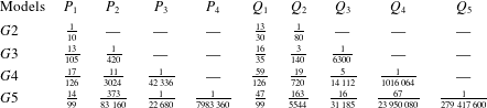
 $$\begin{eqnarray}c_{model}^{2}=\frac{\unicode[STIX]{x1D714}^{2}}{k^{2}}=gd\frac{\displaystyle 1+\mathop{\sum }_{i=1}^{K-1}P_{i}\unicode[STIX]{x1D705}^{2i}}{\displaystyle 1+\mathop{\sum }_{j=1}^{K}Q_{j}\unicode[STIX]{x1D705}^{2j}},\end{eqnarray}$$
where  $P_{i}$ and
 $Q_{j}$ are constant coefficients which are summarized in table 1 for
 $G2$ to
 $G5$ models.
The linear frequency dispersion expressions for the subdomain model are much more complex because of the presence of free parameter(s). For example, for the  $S2$ model the coefficients in the general expression equation, (3.8), are
 $$\begin{eqnarray}P_{1}={\textstyle \frac{1}{12}}(-c_{1}^{2}+c_{1}+1),\quad Q_{1}={\textstyle \frac{1}{12}}(-c_{1}^{2}+c_{1}+5),\quad Q_{2}={\textstyle \frac{1}{72}}(-2c_{1}^{2}+c_{1}+1),\end{eqnarray}$$
where  $c_{1}$ is the free parameter, representing the interface location of the subdomains and needs to be determined later. For the
 $S3$ model, these coefficients in (3.8) become increasingly complex
 $$\begin{eqnarray}\displaystyle \left.\begin{array}{@{}c@{}}\displaystyle P_{1}={\textstyle \frac{1}{60}}(-3c_{1}^{2}+2c_{1}(c_{2}+1)-3c_{2}^{2}+2c_{2}+7),\\ \displaystyle P_{2}={\textstyle \frac{1}{720}}(3c_{1}^{2}(c_{2}^{2}-c_{2}-1)+c_{1}(-3c_{2}^{2}+c_{2}+4)+(4-3c_{2})c_{2}),\\ \displaystyle Q_{1}={\textstyle \frac{1}{60}}(-3c_{1}^{2}+2c_{1}(c_{2}+1)-3c_{2}^{2}+2c_{2}+27),\\ \displaystyle Q_{2}={\textstyle \frac{1}{240}}(c_{1}^{2}(c_{2}^{2}-c_{2}-5)+c_{1}(-c_{2}^{2}+3c_{2}+4)-5c_{2}^{2}+4c_{2}+4),\\ \displaystyle Q_{3}=\frac{(c_{1}-1)(c_{2}-1)(2c_{1}c_{2}+c_{1}+c_{2})}{1440},\end{array}\right\} & & \displaystyle\end{eqnarray}$$
where  $c_{1}$ and
 $c_{2}$ are both free parameters to be specified. The full expressions of linear frequency dispersion for all models (i.e.,
 $G2$–
 $G5$ and
 $S2$–
 $S5$) are provided in § C of the supplementary materials.
Coefficients in the Galerkin models’ linear frequency dispersion relation, (3.8).

In the framework of linear wave theory, the wave group velocity is a measure of the speed of wave energy propagation and can be expressed as
 $$\begin{eqnarray}c_{g}=nc=\frac{1}{2}\left(1+\frac{2\unicode[STIX]{x1D705}}{\sinh 2\unicode[STIX]{x1D705}}\right)c.\end{eqnarray}$$
The wave group velocity associated with the model equations is obtained by differentiating the frequency dispersion relation, (3.8), with respect to  $k$, yielding the following general form:
 $$\begin{eqnarray}n=\frac{1+\displaystyle \mathop{\sum }_{i=1}^{K}P_{i}^{c_{g}}\unicode[STIX]{x1D705}^{2i}}{1+\displaystyle \mathop{\sum }_{j=1}^{K+1}Q_{j}^{c_{g}}\unicode[STIX]{x1D705}^{2j}},\end{eqnarray}$$
where  $P_{i}^{c_{g}}$ and
 $Q_{j}^{c_{g}}$ have analytical forms and the full expressions can be provided in § C of supplementary materials.
The wave shoaling effect becomes important when water depth varies significantly within a wavelength. The linear shoaling gradient is another important quantity in determining the applicability of the present models, which is defined as
 $$\begin{eqnarray}\frac{A_{x}}{A}=\unicode[STIX]{x1D6FE}\frac{d_{x}}{d},\end{eqnarray}$$
where  $A$ is the local wave amplitude and
 $d$ is the water depth, respectively. The subscript
 $x$ denotes the corresponding spatial derivatives. The analytical solution for the shoaling gradient,
 $\unicode[STIX]{x1D6FE}$, based on linear wave theory is,
 $$\begin{eqnarray}\unicode[STIX]{x1D6FE}=-\unicode[STIX]{x1D705}\tanh (\unicode[STIX]{x1D705})\frac{[1-\unicode[STIX]{x1D705}\tanh (\unicode[STIX]{x1D705})][1-\tanh ^{2}(\unicode[STIX]{x1D705})]}{\{\tanh (\unicode[STIX]{x1D705})+\unicode[STIX]{x1D705}[1-\tanh ^{2}(\unicode[STIX]{x1D705})]\}^{2}}.\end{eqnarray}$$
Following Schäffer & Madsen (Reference Schäffer and Madsen1995) and Lynett & Liu (Reference Lynett and Liu2004a) the linear shoaling gradients embedded in the model equations are derived, and they are provided in § C of the supplementary materials for their lengthy expressions.
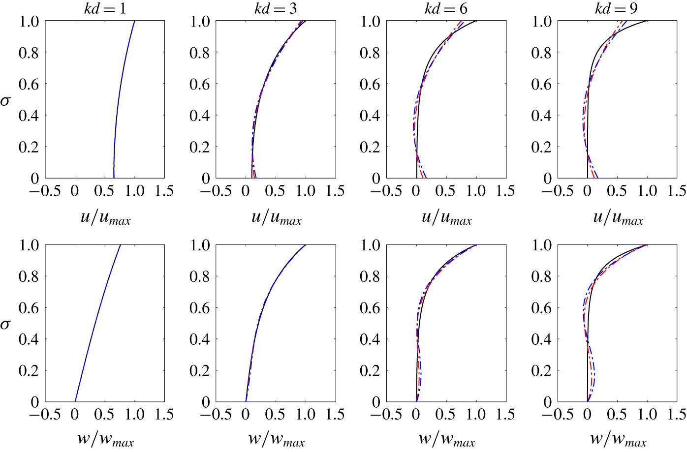
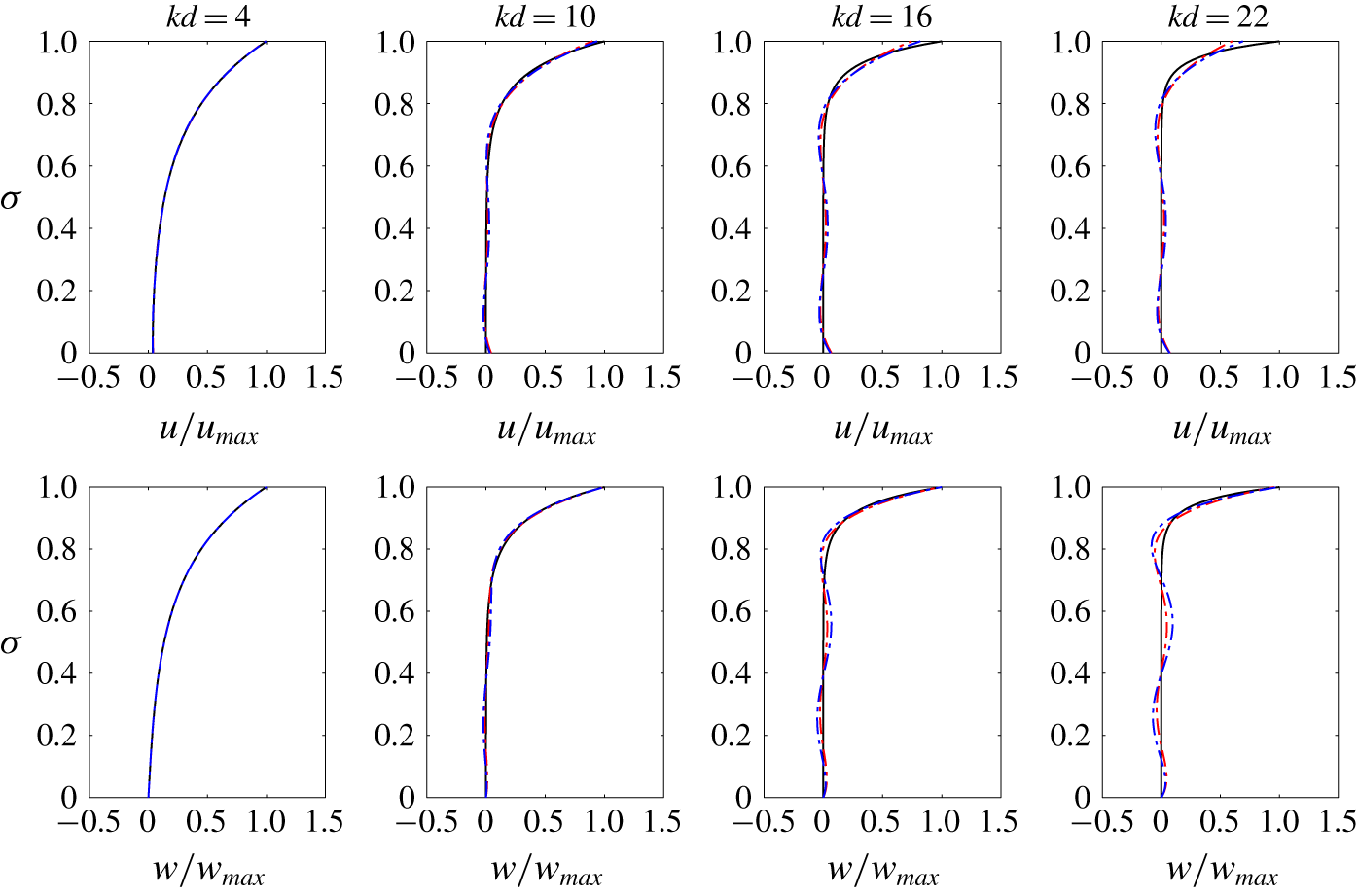
The orbital velocity field plays a critical role in transport processes and in calculating dynamic pressures in the water column. Therefore, the vertical profiles of the horizontal and vertical velocity components obtained from various models are compared with the analytical solutions of linear wave theory, which read
 $$\begin{eqnarray}\displaystyle \left.\begin{array}{@{}c@{}}\displaystyle u^{Stokes}=a_{1}\sqrt{\frac{g}{d}}\sqrt{\unicode[STIX]{x1D705}\tanh \unicode[STIX]{x1D705}}\frac{\cosh k(z+d)}{\sinh \unicode[STIX]{x1D705}}\cos \unicode[STIX]{x1D703},\\ \displaystyle w^{Stokes}=a_{1}\sqrt{\frac{g}{d}}\sqrt{\unicode[STIX]{x1D705}\tanh \unicode[STIX]{x1D705}}\frac{\sinh k(z+d)}{\sinh \unicode[STIX]{x1D705}}\sin \unicode[STIX]{x1D703},\end{array}\right\} & & \displaystyle\end{eqnarray}$$
in Cartesian coordinates.
For the Galerkin models, analytical expressions for all the linear properties mentioned above can be directly compared with the expressions for the linear wave theory. However, for the subdomain model, the free parameters need to be determined. A total model error  $E_{total}$, similar to that of Lynett & Liu (Reference Lynett and Liu2004a), can be defined as the combination of errors induced by linear frequency dispersion, group velocity, integrated shoaling gradient, horizontal and vertical velocity profiles,
 $$\begin{eqnarray}\displaystyle E_{total} & = & \displaystyle \overline{E_{c}}+\overline{E_{c_{g}}}+\overline{E_{shoal}}+\overline{E_{u}}+\overline{E_{w}}\nonumber\\ \displaystyle & = & \displaystyle \overline{\int _{0}^{\unicode[STIX]{x1D6FA}}\left|\frac{[c_{m}^{2}(\unicode[STIX]{x1D705})-c_{e}^{2}(\unicode[STIX]{x1D705})]W}{c_{e}^{2}(\unicode[STIX]{x1D705})}\right|\,\text{d}\unicode[STIX]{x1D705}}+\overline{\int _{0}^{\unicode[STIX]{x1D6FA}}\left|\frac{[{c_{g}}_{m}(\unicode[STIX]{x1D705})-{c_{g}}_{e}(\unicode[STIX]{x1D705})]W}{{c_{g}}_{e}(\unicode[STIX]{x1D705})}\right|\,\text{d}\unicode[STIX]{x1D705}}\nonumber\\ \displaystyle & & \displaystyle +\,\overline{\text{exp}\left[\int _{0}^{\unicode[STIX]{x1D6FA}}\frac{(\unicode[STIX]{x1D6FE}_{e}-\unicode[STIX]{x1D6FE}_{m})W}{\unicode[STIX]{x1D705}}\,\text{d}\unicode[STIX]{x1D705}\right]-1}+\,\overline{\int _{0}^{\unicode[STIX]{x1D6FA}}\int _{0}^{1}\left|\frac{u_{m}(\unicode[STIX]{x1D70E})-u_{e}(\unicode[STIX]{x1D70E})}{u_{e}(1)}\right|\,\text{d}\unicode[STIX]{x1D70E}W\,\text{d}\unicode[STIX]{x1D705}}\nonumber\\ \displaystyle & & \displaystyle +\,\overline{\int _{0}^{\unicode[STIX]{x1D6FA}}\int _{0}^{1}\left|\frac{w_{m}(\unicode[STIX]{x1D70E})-w_{e}(\unicode[STIX]{x1D70E})}{w_{e}(1)}\right|\,\text{d}\unicode[STIX]{x1D70E}W\,\text{d}\unicode[STIX]{x1D705}},\end{eqnarray}$$
where the overbar denotes the normalization by each error’s median value.  $\unicode[STIX]{x1D6FA}$ is the upper limit of the range of
 $\unicode[STIX]{x1D705}$ considered, which is determined on a trial and error basis by achieving possibly largest
 $\unicode[STIX]{x1D705}$ values for overall accuracy without sacrificing local accuracy significantly. Subscripts
 $m$ and
 $e$ denote the model solutions and exact analytical linear solutions, respectively. The weighting function,
 $W=\text{exp}[(2^{-\unicode[STIX]{x1D705}}-2^{-\unicode[STIX]{x03C0}})\log 5]$, is designed to be exponentially decaying with respect to
 $\unicode[STIX]{x1D705}$ to address the importance of shallower water regimes and to avoid possible large local errors. Finally, the definition of the integrated shoaling gradient error,
 $E_{shoal}$, is taken from Chen & Liu (Reference Chen and Liu1995). We remark that the definition of
 $E_{total}$ is not unique and the performance of the optimized value needs to be further checked with numerical validations. Here, only the errors associated with the linear wave properties are considered.
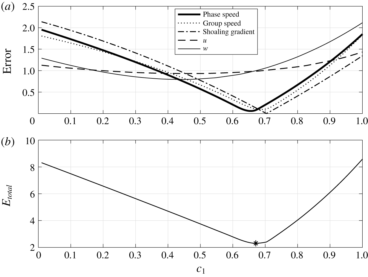
Error versus free parameter  $c_{1}$ for the
 $S2$ model; the asterisk symbol in panel (b) denotes the location of the optimized value.

Figure 1 shows the general behaviour of each error (a) and the total error  $E_{total}$ (b) versus the free parameter
 $c_{1}$ for
 $S2$ model. The phase speed, group speed and the integrated shoaling gradient are relatively sensitive to the choice of the free parameter and the optimal values are located at around
 $c_{1}=0.70$. However, the optimal
 $c_{1}$ values for the vertical profiles of horizontal and vertical velocity are smaller than 0.7. Fortunately, the error variations of both horizontal and vertical velocity profiles are relatively insensitive to the
 $c_{1}$ value. Thus, the optimized free parameter
 $c_{1}=0.672$ is determined by minimizing
 $E_{total}$ in (3.16) for the
 $S2$ model. The same procedure is performed on other models of higher degree of polynomial approximation and the optimized free parameters and
 $\unicode[STIX]{x1D6FA}$ value are summarized in table 2.
Optimized free parameters for the subdomain model  $(SK)$.

The comparisons of the  $GK$ and
 $SK$ model solutions for the normalized wave phase speed, normalized wave group speed and integrated shoaling gradient error are shown in figure 2. All model solutions of the above mentioned linear wave properties become smaller than the exact analytical solutions as water depth becomes deeper (i.e., larger
 $kd$). Thus, half of the vertical coordinate (i.e., the upper part of panel a and b, the lower part of panel c) in figure 2 is reversed for better visualization. It is not surprising that the higher degree of polynomial approximation provides more accurate wave properties as compared to those of linear waves. However, while the wave properties of the
 $GK$ models (denoted as dash-dotted lines) approach monotonically those of linear waves from deep water to shallow water, the wave properties of
 $SK$ models (denoted as lines) show small undulations in certain ranges of
 $kd$ values. For the same degree of polynomial approximation, the
 $SK$ model always has a higher accuracy than the
 $GK$ model does (same colour in the figure). In the same figure, the linear wave properties of the
 $O(\unicode[STIX]{x1D707}^{2})$ Boussinesq-type model (Nwogu Reference Nwogu1993) and the
 $O(\unicode[STIX]{x1D707}^{2})$ two-layer Boussinesq model (Lynett & Liu Reference Lynett and Liu2004a) are also plotted. The model solution of the linear wave phase velocity of the one-layer Boussinesq-type model becomes larger than the exact analytical solution as water becomes deeper. Thus, it is plotted as
 $(2-c_{Nwogu}/c_{e})$ for better visualization in figure 2(a). It is clear that the accuracy of Nwogu’s Boussinesq model is similar to that of the
 $G2$ model but is worse than that of the
 $S2$ model. The two-layer Boussinesq model significantly improves the accuracy of the one-layer Boussinesq model and reaches a similar accuracy to the
 $G3$ model. By specifying an error bound of 2 % for each linear property in figure 2, the upper limits of applicable
 $kd$ values are summarized in table 3 for both
 $GK$ and
 $SK$ models. The applicable range of
 $kd$ values for the
 $SK$ model is approximately 50 %–70 % larger than that for the
 $GK$ model in terms of three listed linear wave properties.
Comparisons of linear wave properties (black:  $G2$ and
 $S2$; green:
 $G3$ and
 $S3$; red:
 $G4$ and
 $S4$; blue:
 $G5$ and
 $S5$); – ⋅ – ⋅ –, Galerkin model (
 $GK$); ——, subdomain model (
 $SK$);
 $O(\unicode[STIX]{x1D707}^{2})$ Boussinesq-type model (Nwogu Reference Nwogu1993) and
 $O(\unicode[STIX]{x1D707}^{2})$ two-layer Boussinesq model (Lynett & Liu Reference Lynett and Liu2004a) are also shown for comparisons.

Applicable upper limits of  $kd$ for the
 $SK$ models and the
 $GK$ models (in the brackets) in terms of linear properties. The error bound is set at 2 %.

The ratio between the velocity coefficients,  $u_{i1}$ and wave amplitude,
 $a_{1}$ can be obtained by solving the first-order homogeneous equation system, (3.5). Thus, the horizontal velocity profile can be reconstructed for
 $GK$ and
 $SK$ models, respectively. The comparisons between model solutions and the analytical solutions for the horizontal and vertical velocity, being normalized by the analytical surface velocity (
 $u_{max}$ and
 $w_{max}$), are presented for different
 $kd$ values in figures 3 and 4. The model solutions obtained by
 $G3$ and
 $S3$ are shown in figure 3, while
 $G5$ and
 $S5$ solutions are shown in figure 4. Overall, all models give reasonable velocity profiles within the upper limit of
 $kd$ values for each model (see table 3). However, for the horizontal velocity, both models underestimate surface velocity and overestimate bottom velocity for high
 $kd$ values. The horizontal velocity in
 $K=3$ models has a quadratic structure in the vertical direction, which is the same as the
 $O(\unicode[STIX]{x1D707}^{2})$ one-layer Boussinesq-type model. However, the vertical structure of the vertical velocity in
 $K=3$ models is a cubic polynomial in the present models, while in the Boussinesq-type models the vertical velocity has a linear vertical profile. Finally, although the velocity profiles obtained from the subdomain models show slightly larger error in the lower part of the water column in comparison with the Galerkin model, the subdomain models always provide better predictions on the velocity profile near the free surface. This is probably the reason why the subdomain model demonstrates better linear frequency dispersion accuracy over the Galerkin model for the same degree of polynomial approximation.
Normalized velocity profiles are plotted for different  $kd$ values: (blue:
 $S3$; red:
 $G3$; black: analytical solution).

Normalized velocity profiles are plotted for different  $kd$ values: (blue:
 $S5$; red:
 $G5$; black: analytical solution).

3.1.3 Second- and third-order solutions
In this section, the second- and third-order nonlinear effects embedded in the model equations are examined and compared with the analytical solutions.
To solve for  $a_{2}$, the
 $O(\unicode[STIX]{x1D716}^{2})$ equations are obtained after substituting the Stokes-type expansions into the governing equations. For example, for the
 $S2$ model the resulting equations can be organized in the form of (3.5). However, the forcing terms on the right-hand side are no longer zero. The analytical expressions for
 $a_{2}$ for the Galerkin models can be obtained in terms of
 $a_{1}$ and
 $kd$. The second-order amplitude will be compared with the corresponding analytical solution for Stokes waves (e.g., Skjelbreia & Hendrickson Reference Skjelbreia and Hendrickson1960), which is expressed as
 $$\begin{eqnarray}a_{2}^{Stokes}=\frac{k{a_{1}}^{2}}{4}[3\coth ^{3}\unicode[STIX]{x1D705}-\coth \unicode[STIX]{x1D705}].\end{eqnarray}$$
After some manipulation the second-order wave amplitude based on  $G2$ model can be written as
 $$\begin{eqnarray}a_{2}^{G2}=\frac{{a_{1}}^{2}k(31\unicode[STIX]{x1D705}^{8}+683\unicode[STIX]{x1D705}^{6}+4230\unicode[STIX]{x1D705}^{4}+11\,200\unicode[STIX]{x1D705}^{2}+12\,000)}{4\unicode[STIX]{x1D705}^{3}(\unicode[STIX]{x1D705}^{2}+10)(6\unicode[STIX]{x1D705}^{4}+75\unicode[STIX]{x1D705}^{2}+400)}.\end{eqnarray}$$
Comparisons of nonlinear properties (black:  $G2$ and
 $S2$
; green:
 $G3$ and
 $S3$; red:
 $G4$ and
 $S4$; blue:
 $G5$ and
 $S5$): – ⋅ – ⋅ –, Galerkin model (
 $GK$); ——, subdomain model (
 $SK$).

The analytical solutions for the third-order Stokes waves are (e.g., Skjelbreia & Hendrickson Reference Skjelbreia and Hendrickson1960)
 $$\begin{eqnarray}\displaystyle & \displaystyle a_{3}^{Stokes}=\frac{3}{64}a_{1}^{3}k^{2}\frac{1+8\cosh ^{6}(\unicode[STIX]{x1D705})}{\sinh ^{6}(\unicode[STIX]{x1D705})}, & \displaystyle\end{eqnarray}$$
 $$\begin{eqnarray}\displaystyle & \displaystyle \unicode[STIX]{x1D714}_{13}^{Stokes}=\frac{1}{16}a_{1}^{2}k^{2}\frac{9\tanh ^{4}(\unicode[STIX]{x1D705})-10\tanh ^{2}(\unicode[STIX]{x1D705})+9}{\tanh ^{4}(\unicode[STIX]{x1D705})}. & \displaystyle\end{eqnarray}$$
Similarly, the third-order wave amplitude  $a_{3}$ and the wave frequency
 $\unicode[STIX]{x1D714}_{13}$ can be obtained by solving
 $O(\unicode[STIX]{x1D716}^{3})$ model equations. For the
 $G2$ model, the third-order wave amplitude
 $a_{3}^{G2}$ and amplitude dispersion
 $\unicode[STIX]{x1D714}_{13}^{G2}$ are
 $$\begin{eqnarray}a_{3}^{G2}=a_{1}^{3}k^{2}\frac{P_{3}^{G2}}{Q_{3}^{G2}},\end{eqnarray}$$
where
 $$\begin{eqnarray}\displaystyle P_{3}^{G2} & = & \displaystyle 172\,863\unicode[STIX]{x1D705}^{14}+5347\,038\unicode[STIX]{x1D705}^{12}+57\,290\,112\unicode[STIX]{x1D705}^{10}+308\,253\,920\unicode[STIX]{x1D705}^{8}\nonumber\\ \displaystyle & & \displaystyle +\,965\,721\,600\unicode[STIX]{x1D705}^{6}+1727\,616\,000\unicode[STIX]{x1D705}^{4}+1566\,720\,000\unicode[STIX]{x1D705}^{2}+691\,200\,000,\quad\end{eqnarray}$$
 $$\begin{eqnarray}Q_{3}^{G2}=512\unicode[STIX]{x1D705}^{6}(\unicode[STIX]{x1D705}^{2}+10)(6\unicode[STIX]{x1D705}^{4}+75\unicode[STIX]{x1D705}^{2}+400)(27\unicode[STIX]{x1D705}^{4}+300\unicode[STIX]{x1D705}^{2}+800),\end{eqnarray}$$
and
 $$\begin{eqnarray}\unicode[STIX]{x1D714}_{13}^{G2}=a_{1}^{2}k^{2}\frac{P_{13}^{G2}}{Q_{13}^{G2}},\end{eqnarray}$$
where
 $$\begin{eqnarray}\displaystyle P_{13}^{G2} & = & \displaystyle 11\,523\unicode[STIX]{x1D705}^{14}+647\,334\unicode[STIX]{x1D705}^{12}+11\,383\,968\unicode[STIX]{x1D705}^{10}+94\,191\,840\unicode[STIX]{x1D705}^{8}\nonumber\\ \displaystyle & & \displaystyle +\,402\,265\,600\unicode[STIX]{x1D705}^{6}+790\,144\,000\unicode[STIX]{x1D705}^{4}+706\,560\,000\unicode[STIX]{x1D705}^{2}+691\,200\,000,\end{eqnarray}$$
 $$\begin{eqnarray}Q_{13}^{G2}=128\unicode[STIX]{x1D705}^{4}(\unicode[STIX]{x1D705}^{2}+10)^{2}(3\unicode[STIX]{x1D705}^{4}+104\unicode[STIX]{x1D705}^{2}+240)(6\unicode[STIX]{x1D705}^{4}+75\unicode[STIX]{x1D705}^{2}+400).\end{eqnarray}$$
The second- and third-order model solutions using higher polynomial approximations with the exception of the  $S5$ model are also available in § C of the supplementary materials. Figure 5 displays the nonlinear properties of various
 $GK$ and
 $SK$ models, using the corresponding optimized parameter(s) listed in table 2. Similar to the linear wave properties, all the model solutions of the above mentioned nonlinear wave properties are becoming smaller than the exact analytical solutions as water depth becomes deeper (i.e., larger
 $kd$). Thus, half of the vertical coordinate (i.e., the upper part of each panel) in figure 5 is reversed for better visualization. The higher degree of polynomial approximation always has higher accuracy for all the nonlinear properties for both types of models. And the
 $SK$ models (dash-dotted line) demonstrate better skills than the
 $GK$ models (thick line) for the same degree of polynomial approximation. Similar to the analysis for linear wave properties, the upper limits of applicable
 $kd$ value are summarized together in table 4. Larger error bounds (5 % or 10 %) are used for evaluating the nonlinear properties in table 4, because nonlinearity is usually considered to be small and its impact on simulating wave field is less significant than the linear properties. The
 $S3$ model already shows good nonlinear behaviour even up to the deep water limit (
 $kd\approx \unicode[STIX]{x03C0}$) with less than
 $5\,\%$ error in the second-order wave amplitude. Although nonlinear properties are not considered in the parameter optimization for the subdomain model, the above analysis demonstrates the subdomain model still processes reasonable nonlinear accuracy using the parameters obtained from linear optimization.
Applicable upper limits of  $kd$ for the
 $SK$ models and the
 $GK$ models (in the brackets) in terms of nonlinear properties.

3.2 Wave–current interactions – Doppler shift effect
It is well known that the Boussinesq-type models cannot include appreciable horizontal vorticities, such as vertically sheared currents. On the other hand, the skill of the present models in simulating vertically sheared currents hinges on the degree of polynomial approximation in the vertical structure of the velocity fields. In this section, we shall examine this aspect quantitatively.
The linear wave frequency dispersion relation is modified when the wave propagates in an ambient current field, and the Doppler shift effect is the most direct consequence. For example, the analytical expression for the modified frequency dispersion relation with a linearly sheared current (e.g., Thompson Reference Thompson1949; Nwogu Reference Nwogu2009) is
 $$\begin{eqnarray}c-U_{0}=-\frac{\unicode[STIX]{x1D6E9}}{2k}\tanh \unicode[STIX]{x1D705}\pm \sqrt{\left(\frac{\unicode[STIX]{x1D6E9}}{2k}\tanh \unicode[STIX]{x1D705}\right)^{2}+\frac{g}{k}\tanh \unicode[STIX]{x1D705}},\end{eqnarray}$$
where  $c$ is the phase speed,
 $U_{0}$ is the current velocity on the free surface, and
 $\unicode[STIX]{x1D6E9}$ represents the constant shear. It should be noted that the Doppler shift effect under a uniform current can be recovered by setting
 $\unicode[STIX]{x1D6E9}=0$ in the above equation.
The expansions for the total water depth and horizontal velocity for combined wave–current solutions in Cartesian coordinates can be expressed as
 $$\begin{eqnarray}\displaystyle & \displaystyle H=d+\unicode[STIX]{x1D716}a_{1}\cos \unicode[STIX]{x1D703}, & \displaystyle\end{eqnarray}$$
 $$\begin{eqnarray}\displaystyle & \displaystyle u=\unicode[STIX]{x1D716}u_{w}\cos \unicode[STIX]{x1D703}+U_{0}+\unicode[STIX]{x1D6E9}z, & \displaystyle\end{eqnarray}$$
where  $U_{0}$ and
 $\unicode[STIX]{x1D6E9}$ are prescribed, and
 $u_{w}$ denotes the amplitude of the periodic orbital motion of linear waves. The combined wave and current solution, (3.29), is further approximated based on the specific velocity assumption before substituting it into the model equations to be examined. The procedure is similar to that presented in § 3.1.2 for pure waves. By collecting terms that are linear in terms of
 $\unicode[STIX]{x1D716}$ in the resulting equations, the linear wave frequency dispersion relation in the presence of linearly sheared current can be obtained by solving a matrix equation in the form of (3.5).
Comparisons of solutions of Doppler shift relation given by linear Stokes theory (black lines),  $G2$ model (red lines) and
 $S2$ model (blue lines) for seven different
 $d/L_{0}$ values.

For the uniform current (i.e.,  $\unicode[STIX]{x1D6E9}=0$), the modified linear wave frequency dispersion for all model equations derived in this paper can be expressed as
 $$\begin{eqnarray}\frac{(\unicode[STIX]{x1D714}-kU_{0})^{2}}{k^{2}}=gd\frac{1+\displaystyle \mathop{\sum }_{i=1}^{K-1}P_{i}\unicode[STIX]{x1D705}^{2i}}{1+\displaystyle \mathop{\sum }_{j=1}^{K}Q_{j}\unicode[STIX]{x1D705}^{2j}},\end{eqnarray}$$
where  $P_{i}$ and
 $Q_{j}$ are exactly the same as the expressions shown in (3.8) for pure waves. Thus, the Doppler shift effect of a uniform current is indeed embedded in all models. On the other hand, for Boussinesq-type models, only the higher nonlinear version can reproduce such Doppler shift effect (Yoon & Liu Reference Yoon and Liu1989; Chen et al. Reference Chen, Madsen, Schäffer and Basco1998). Following Madsen & Schäffer (Reference Madsen and Schäffer1998) and Chen et al. (Reference Chen, Madsen, Schäffer and Basco1998), the range of applicability of present models for wave and current interactions is investigated. The Doppler shift relation, (3.30), is further represented as the non-dimensional wavenumber
 $(kd)$ versus the Froude number (
 $Fr$) for different values of
 $d/L_{0}$, which are defined as
 $$\begin{eqnarray}Fr=\frac{U_{0}}{\sqrt{gd}},\quad \frac{d}{L_{0}}=\frac{\unicode[STIX]{x1D714}^{2}d}{2\unicode[STIX]{x03C0}g},\end{eqnarray}$$
where  $L_{0}$ is the deep water wavelength without current. Figure 6 shows the comparison of solutions from Doppler shift relation of
 $G2$ model,
 $S2$ model and linear analytical solution (
 $\unicode[STIX]{x1D6E9}=0$), (3.27), for seven different values of
 $d/L_{0}$. For the opposing current situations (
 $Fr<0$), present models gradually lose their accuracy with an increasing magnitude of the Froude number, but the error is generally small for relatively small
 $d/L_{0}$ values. Also it is the opposite for the following current situations as larger Froude numbers result in better accuracy. Finally, it is not surprising that the
 $S2$ model always performs better than the
 $G2$ model as the former one is more accurate in terms of linear wave dispersion relation.
For linearly sheared currents, figure 7 shows the wave phase velocity, normalized by the exact solution, (3.27), for the  $G2$ model (a) and the
 $S2$ model (b), respectively. Again, half of the vertical coordinate (i.e., the upper part of each panel) in figure 7 is reversed for better visualization. In fact, models using higher degree of polynomial approximation show similar behaviour. In each panel, the upper and lower part compare normalized linear wave frequency dispersion relation for the following (wave and current are in the same direction) and opposing (wave and current are in the opposite direction) current, respectively. The dimensionless parameter
 $S=\unicode[STIX]{x1D6E9}\text{d}/\sqrt{g\text{d}}$ indicates the strength and direction of the vertical shear;
 $S=-0.4$,
 $-0.2$, 0, 0.2 and 0.4 are selected as examples. The linear wave frequency dispersion under linearly sheared current is well approximated within the applicable range of
 $kd$ values of the pure wave scenarios (see table 3). Behaviour of these model solutions for larger
 $kd$ values can be summarized as follows: (i) relative to the pure wave situation, the linear frequency dispersion associated with the models shows better accuracy for following currents with larger negative shear; (ii) the model’s linear frequency dispersion is less accurate for following currents with larger positive shear; (iii) for the opposing currents the behaviour of linear frequency dispersion embedded in the models is just the opposite.
Normalized linear frequency dispersion for waves with sheared current for the  $G2$ model (a) and
 $S2$ model (b): red dotted,
 $S=-0.4$; red dashed,
 $S=-0.2$; black,
 $S=0.0$; blue dashed,
 $S=0.2$; blue dotted,
 $S=0.4$.

4 Comparisons between model solutions and experimental data
In this section, the present mathematical models are implemented numerically and are then checked with several benchmark experiments and newly conducted laboratory experiments. In the numerical model, a five-point finite differencing is used for spatial discretization, while the modified fourth-order Runge–Kutta scheme (Pike & Roe Reference Pike and Roe1985) is applied for temporal integration to reduce the requirement of virtual storage. Both the Galerkin and the subdomain models of different degree of polynomial approximation (i.e.,  $G2{-}G5$ and
 $S2{-}S5$) have been tested for all cases discussed in this section.
4.1 Wave transformation over a submerged bar with mild slopes
Experimental set-up and gauge locations (in m) for wave transformation over a submerged bar with mild slopes (Dingemans Reference Dingemans1994).

Comparisons among numerical results from  $G2$ model (black line),
 $S2$ model (blue line) and experimental data (red circles).

Comparisons among numerical results from  $G4$ model (black line) and
 $S3$ model (blue line) with the experimental data (red circles). Note that black and blue lines are not differentiable.

Wave transformation over a submerged bar has been a standard test case for many depth-averaged models (Beji & Battjes Reference Beji and Battjes1994; Gobbi & Kirby Reference Gobbi and Kirby1999; Lynett & Liu Reference Lynett and Liu2004a; Liang et al. Reference Liang, Wu, Liu, Fan and Li2015). The set-up of numerical experiments mimics the laboratory experiment by Dingemans (Reference Dingemans1994). A submerged bar with a front slope of  $1/20$ and a back slope of
 $1/10$ is placed in the middle of wave flume with a still water depth of
 $0.86~\text{m}$ (figure 8). The incident wave amplitude is
 $0.02~\text{m}$ with a period of
 $2.86~s$, representing a small amplitude wave propagating in a finite water depth of
 $kd\approx 0.7$ with a weak nonlinearity of
 $ka\approx 0.016$. The wave train shoals up the front slope and the nonlinearity becomes increasingly important. Both sub-harmonics and super-harmonics are generated due to the nonlinear effects. Some of the higher harmonic waves, appearing behind the bar, are in the deep water condition.
In the numerical models, analytical solutions of free surface elevation together with horizontal velocity, corresponding to the incident waves, are provided as the boundary condition at the left boundary, and a sponge layer absorber of  $20~\text{m}$ long (two to three times of the incident wave wavelength) is implemented at the right end of the computational domain. The spatial resolution of
 $\unicode[STIX]{x0394}x=0.05~\text{m}$, together with a temporal resolution of
 $\unicode[STIX]{x0394}t=0.025~\text{s}$, have been tested to produce the converged numerical results for all models.
Figure 9 shows the comparisons between the numerical results, obtained from the  $G2$ model and the
 $S2$ model, and the experimental data. The agreement is quite good in the region before and on the top of bar, showing that both models are capable of capturing the shoaling process and simulating highly nonlinear waves. However, because the release of higher harmonics into deeper water depth behind the bar, noticeable discrepancies between both the models and the experimental data can be seen immediately after the bar (e.g.,
 $x>30.44~\text{m}$). We also report here that the
 $S2$ model performs better than the
 $G2$ model and the
 $S2$ model’s results are also more accurate than the
 $O(\unicode[STIX]{x1D707}^{2})$ fully nonlinear Boussinesq-type model (Wei et al. Reference Wei, Kirby, Grilli and Subramanya1995).
For this submerged bar case, additional numerical tests show that the  $G4$ model and the
 $S3$ model provide the converged results for each type of model, respectively, meaning that models of higher degree of polynomial approximation (e.g.,
 $G5$ and
 $S4$) do not produce more accurate results. The comparisons of these model results against the experimental data are shown in figure 10. Both models give excellent results at all wave gauges, showing their capability for capturing the effects of nonlinearity and frequency dispersion. The inter-model comparisons also demonstrate that subdomain models are superior to the Galerkin models under the same degree of polynomial approximation, which has already been shown in the theoretical analysis in the previous section. Zhao et al. (Reference Zhao, Duan and Ertekin2014) conducted numerical experiments against this case using the GN models. Good predictions are also obtained, but a model with higher degree of polynomial approximation is required (i.e., GN-5 with a fourth-degree polynomial assumption in the horizontal velocity, which is equivalent to the present
 $G5$ model).
Experimental cases in Ohyama, Kioka & Tada (Reference Ohyama, Kioka and Tada1995).

4.2 Wave transformation over a submerged steep bar with steep slopes
Experimental set-up and gauge locations for wave transformation over a submerged bar with steep slopes (Ohyama et al. Reference Ohyama, Kioka and Tada1995).

Ohyama et al. (Reference Ohyama, Kioka and Tada1995) conducted another set of experiments using a submerged symmetric bar with much steeper slopes (1 in 2 slope) than the one shown in the previous section. The experimental set-up and the locations of wave gauges are sketched in figure 11. In the experiments, the still water depth is  $0.5~\text{m}$. The incident wave conditions are summarized in table 5. There are four cases with different combinations of wave amplitudes and periods; no wave breaking is observed in the experiments. The incident waves in case (1) and (2) are in deeper water and all four cases have larger
 $ka$ values than that of Dingemans (Reference Dingemans1994) shown in the previous section. The spatial and temporal resolutions of numerical simulations for each case are also summarized in the last two columns in table 5. In this problem the slope is relatively steep (1:2). The sudden change of slope at the toe causes numerical noise. A nine-point filter (Shaprio Reference Shaprio1970) is applied to both surface elevations and velocity unknowns every 20–200 time steps to eliminate spurious solutions.
We anticipate that models with higher degree of polynomial approximation are needed for cases (1) and (2) because of their larger  $kd$ and
 $ka$ values. Figure 12 shows the comparisons between numerical results obtained by
 $G2$ and
 $S2$ with experimental data for all cases. As the lowest approximation of each type of model, both the
 $G2$ and the
 $S2$ models are still able to produce accurate solutions for all cases at station 3, which is located at the back edge of the crest of the submerged bar. However, as higher harmonic waves propagate into much deeper water behind the steep slope, both models failed to accurately reproduce the free surface elevations at station 5. Closer observations show that while the
 $G2$ model is very inaccurate at station 5, the
 $S2$ model can still roughly capture the general behaviour of the surface elevations because of its superior wave properties.
Comparisons among numerical results obtained from  $G2$ model (black line),
 $S2$ model (blue line) models and the experimental data (red circles).

Comparisons among numerical results and the experimental data (red circles). Case 1 and 2:  $G5$, black line;
 $S4$, blue line. Case 4 and 6:
 $G4$, black line;
 $S3$, blue line. Note that black and blue lines are not differentiable.

Additional numerical experiments show that the  $G5$ and the
 $S4$ models produce converged results for cases (1) and (2), while the
 $G4$ and the
 $S3$ models provide converged results for cases (4) and (6). The detailed comparisons of the time series of free surface elevations at different locations are given in figure 13. Both models agree with experimental data, demonstrating the model’s ability in treating large water depth variations and stronger nonlinearity. We also find that for cases (2) and (4) present models show better agreement with experimental data than the higher-order (
 $O(\unicode[STIX]{x1D707}^{4})$) Boussinesq model (Gobbi & Kirby Reference Gobbi and Kirby1999) and highly dispersive and highly nonlinear multi-layer Boussinesq model (Liu et al. Reference Liu, Fang and Cheng2018). Present models also produce more accurate results at station 5 in case (4) compared with the GN models presented in Zhao et al. (Reference Zhao, Duan and Ertekin2014).
4.3 Wave and linearly sheared current interactions
One of the significant advantages of the present models over Boussinesq-type models is that the new models have fewer restrictions on the horizontal vorticity, allowing interactions between waves and sheared currents. In this section, the present models are checked with laboratory experiments on interactions of a self-focusing wave group and a sheared current (Chen et al. Reference Chen, Stagonas, Santo, Buldakov, Simons, Taylor and Zang2019).
The experiments were conducted in a 20 m long, 1.2 m wide and 1 m deep recirculating wave–current flume at University College London (UCL) (Chen et al. Reference Chen, Stagonas, Santo, Buldakov, Simons, Taylor and Zang2019). The still water depth of 0.5 m was used in the experiments. Two flow profilers were installed on top of the inlet and the outlet to generate flows with the desired vertical structure. Flow velocities were measured with a particle image velocimetry (PIV) system. Following Buldakov, Stagonas & Simons (Reference Buldakov, Stagonas and Simons2017) and Stagonas, Buldakov & Simons (Reference Stagonas, Buldakov and Simons2018), self-focusing wave groups were generated using a Gaussian spectrum and the designed focal point is located at 8.7 m from the wavemaker for both with and without current cases. The peak frequency was set at 0.6 Hz, corresponding to  $kd\approx 0.968$. Seven wave gauges were used to measure the free surface elevations along the flume with the last one being located at the designed focal point. Detailed experimental set-up can be found in Chen et al. (Reference Chen, Stagonas, Santo, Buldakov, Simons, Taylor and Zang2019).
Linearly sheared current profiles in the experiments in Chen et al. (Reference Chen, Stagonas, Santo, Buldakov, Simons, Taylor and Zang2019): blue, following current; red, opposing current; circles, PIV data; plus sign, ADV data.

The sheared currents measured in the experiments show a co-linear distribution in the vertical water column as shown in figure 14, which corresponds to figure 5 in Chen et al. (Reference Chen, Stagonas, Santo, Buldakov, Simons, Taylor and Zang2019). The PIV data is only available from the still water level to  $z=-0.3~\text{m}$ as shown by circle markers, and the velocity in the lower part was measured by the acoustic Doppler velocimetry (ADV) as denoted by asterisks. The surface velocity of the sheared currents is approximately
 $0.2~\text{m}~\text{s}^{-1}$. The constant vorticities are roughly
 $0.374~\text{s}^{-1}$ for the following current and
 $-0.295~\text{s}^{-1}$ for the opposing current.
Comparisons of free surface elevations for waves alone case: black line, experiment data; blue dashed,  $G3$ model; red dashed,
 $S2$ model. Note that the agreement is excellent and the black, blue and red lines are not differentiable.

Comparisons of free surface elevations for waves on following linearly sheared current case: black line, experiment data; blue dashed,  $G3$ model; red dashed,
 $S2$ model. Note that black, blue and red lines are not differentiable.

Three experimental cases are considered here; namely, waves without current, waves with following sheared current and waves with opposing sheared current. In the numerical experiments, the surface elevations measured at the wave gauge nearest to the wavemaker are used directly as the boundary condition, and the velocity boundary condition is reconstructed from the free surface elevation measurements via the linear wave theory. For the wave–current interaction cases, a steady current, according to the velocity profiles shown in figure 14 is first initiated in the entire computational domain for both boundary and initial conditions. Computations then start by superimposing the wave conditions (free surface elevation and velocity) on the current at the left boundary condition. The numerical model does not distinguish between waves or currents by solving the full velocity field, allowing a complex interaction between waves and currents inside the computation domain. A spatial resolution of  $\unicode[STIX]{x0394}x=0.05~\text{m}$ and temporal resolution of
 $\unicode[STIX]{x0394}t=0.02~\text{s}$ are used for all cases considered here.
Comparisons of free surface elevations for waves on opposing linearly sheared current case: black line, experiment data; blue dashed,  $G3$ model; red dashed,
 $S2$ model. Note that black, blue and red lines are not differentiable.

Numerical experiments show that the  $G3$ and
 $S2$ models are able to produce the converged numerical results in terms of free surface elevations for each type of model. Figures 15, 16 and 17 show the free surface elevation comparisons for the pure waves, waves with following sheared current, and waves with opposing sheared current, respectively. Both the
 $G3$ and
 $S2$ models are able to produce quite good predictions on free surface elevations for all three cases. In order to understand the models’ performances in reproducing the velocity profile, figure 18 shows the comparisons on the vertical profiles of the horizontal velocity for all three cases (i.e., three groups of lines a, b and c) at the instant of focusing at
 $x=8.7~\text{m}$ for the
 $G2$,
 $G3$,
 $S2$ and
 $S3$ models. It is interesting to observe that although the
 $S2$ model can produce accurate free surface elevations, it cannot describe the velocity profiles, especially for the pure waves and waves on opposing current cases, because of its linear horizontal velocity profile approximation. The general behaviour of the
 $G2$ and
 $S2$ models (dash-dotted lines) follows the linear wave velocity profile analysis in § 3.1.2, meaning that the
 $SK$ models have larger but also better estimations than the
 $GK$ models near the free surface, while the
 $GK$ models have smaller but also better estimations than the
 $SK$ models near the bottom. On the other hand, the
 $S3$ and
 $G3$ models (dashed lines) show quite similar results with only slight differences appearing near to the free surface and bottom, the vertical structure is well reproduced by both models for all three cases, which is comparable to the numerical results obtained by the computational fluid dynamics method shown in Chen et al. (Reference Chen, Stagonas, Santo, Buldakov, Simons, Taylor and Zang2019).
4.4 New self-focusing wave package experiments
To further explore the skills of the present models, a new set of self-focusing wave group experiments was conducted in the wave flume ( $36~\text{m}$ in length,
 $2~\text{m}$ in width and
 $1.3~\text{m}$ in depth) at the National University of Singapore (NUS). The wave flume is equipped with a computer-controlled wavemaker in which user-defined time series of free surface elevation are used as input signals. A wave absorption system is installed at the other end of the flume to minimize reflection. Earlier experiments show that the wavemaker is highly repeatable. The maximum variation of the maximum wave height and its corresponding wave period calculated using a zero-crossing method is less than 2 %. The comparison of measured free surface elevations between two separated runs is shown in § D of the supplementary material.
Comparisons of horizontal velocity profiles. (a) Waves on opposing current; (b) waves alone; (c) waves on following current. Blue dash-dotted,  $G2$; blue dashed,
 $G3$; red dash-dotted,
 $S2$; red dashed,
 $S3$.

The incident wave package is a linear summation of 40 evenly spaced sinusoidal wave components over a different range of frequencies. The phase of each wave frequency component is determined by the prescribed focusing location and time within the framework of linear wave theory. The wave amplitude of these wave components follows two different kinds of distribution, i.e., constant wave amplitude ( $a$) and constant wave steepness (
 $ka$). The wave package with constant steepness distribution (smaller wave amplitude accompanied with higher frequency) is expected to generate stable focusing waves with very large amplitudes (Kway, Loh & Chan Reference Kway, Loh and Chan1998), which challenges the abilities of depth-integrated models. On the other hand, the wave energy is evenly distributed within the wave package that has constant amplitude distribution. Thus, the accuracy of the model’s linear frequency can be monitored by changing the frequency range covered by the wave package. Four cases have been carried out in a still water depth of 0.9 m and the target incident wave parameters are summarized in table 6, in which subscripts
 $l$,
 $c$ and
 $h$ denote the corresponding ‘low’, ‘central’ and ‘high’ values, respectively. We remark here that the incident wave packages are designed to be trough focused while the highest wave crest near the focal point is very close to the breaking limit. Free surface elevations are measured by using capacitance wave gauges at eight locations with distances of 4.458 m, 8.013 m, 11.995 m, 13.98 m, 15.27 m, 16.786 m, 19.804 m and 21.2 m to the wavemaker position, respectively. An ADV with a sampling rate of
 $100~\text{Hz}$ is deployed at
 $x=15.27~\text{m}$ and repeated tests are used to measure the time histories of particle velocity at depths of 0.15 m, 0.20 m, 0.25 m, 0.30 m, 0.40 m and
 $0.45~\text{m}$ from the still water level, respectively. For brevity, only the comparisons for cases A1 and B2 are shown here, the comparisons of cases A2 and B1 are provided in § D of the supplementary materials.
Experimental cases for self-focusing wave package at NUS.

Comparisons of surface elevation time series and corresponding amplitude spectra between experimental data (black) and numerical results ( $G5$ model: blue dash-dotted;
 $S4$ model: red dash-dotted) for case A1. Note that black, blue and red lines are not differentiable.

For case A1, the incident wave group is constructed with a constant wave steepness spectrum and it covers a wide range of  $kd$ from 1.12 to 8.15 with a central value of
 $kd\approx 3.63$. In the numerical simulations, the free surface elevations measured at the wave gauge nearest to the wavemaker
 $(x=4.458~\text{m})$ are used as the input boundary condition directly. The free surface measurements are also converted into the horizontal velocities in the water column using the linear wave theory, which is in turn used as the boundary condition. A spatial resolution of
 $\unicode[STIX]{x0394}x=0.04~\text{m}$ and temporal resolution
 $\unicode[STIX]{x0394}t=0.025~\text{s}$ are used in the numerical simulations. The numerical experiments show that while the
 $G5$ model produces the converged results, the solutions from the
 $S4$ model are already converged for this case because of its superior linear frequency dispersion property.
Figure 19 compares numerical results obtained from the  $G5$ model and the
 $S4$ model against experimental data for the free surface elevations and corresponding amplitude spectra. Focusing (
 $x=8.013~\text{m}$ to
 $x=15.27~\text{m}$) and de-focussing (
 $x=16.786~\text{m}$ to
 $x=21.20~\text{m}$) processes of the wave group can be observed from the free surface elevation measurements at these six wave gauges. Very good agreement for both free surface elevations and amplitude spectra at all gauges is observed; the present models are not only able to capture a few centimetre small surface fluctuations but also to reproduce large waves of more than 10 cm at
 $x=15.27~\text{m}$ and 16.786 m, respectively. Furthermore, the evolution of the spectra shows that more high-frequency waves are being generated in the focusing phase and then revert back to the initial spectra shape during the de-focusing phase. Similar recurrence phenomena have been observed in previous experiments on nonlinear waves in deep water (Lake et al. Reference Lake, Yuen, Rungaldier and Ferguson1977; Waseda & Tulin Reference Waseda and Tulin1999; Hwung, Chiang & Hsiao Reference Hwung, Chiang and Hsiao2007).
Comparisons of horizontal velocity in the water column (at  $x=15.27~\text{m}$) between experimental data (black) and numerical results (
 $G5$ model: blue dash-dotted;
 $S4$ model: red dash-dotted) for case A1.

Comparisons of vertical velocity in the water column (at  $x=15.27~\text{m}$) between experimental data (black) and numerical results (
 $G5$ model: blue dash-dotted;
 $S4$ model: red dash-dotted) for case A1.

Comparisons of surface elevation time series and corresponding amplitude spectra between experimental data (black) and numerical results ( $G5$ model: blue dash-dotted;
 $S4$ model: red dash-dotted) for case B2. Note that black, blue and red lines are not differentiable.

Comparisons of horizontal velocity in the water column (at  $x=15.27~\text{m}$) between experimental data (black) and numerical results (
 $G5$ model: blue dash-dotted;
 $S4$ model: red dash-dotted) for case B2.

Comparisons of vertical velocity in the water column (at  $x=15.27~\text{m}$) between experimental data (black) and numerical results (
 $G5$ model: blue dash-dotted;
 $S4$ model: red dash-dotted) for case B2.

Figures 20 and 21 show the comparisons of the time series of horizontal velocity and vertical velocity between the ADV measurements and numerical results at six different elevations in the water column at  $x=15.27~\text{m}$. It should be noted that the ADV data shown here is the raw data (100
 $~\text{Hz}$) without filtering. Very good agreement is observed at all elevations.
The wave boundary conditions in the B2 case follow a constant amplitude distribution. The frequency in the B2 wave package ranges from  $0.5~\text{Hz}$ to 1.5 Hz, corresponding to
 $kd\approx 0.27$ to 5.22 in a water depth of 0.9 m, covering shallow, intermediate and deep water regimes. The same spatial and temporal resolutions are used in the numerical simulation for this case as in case A1. Figures 22, 23 and 24 show the comparison between experimental data and numerical results (
 $G5$ and
 $S4$ models only) for the surface elevation together with the amplitude spectra, horizontal velocity and vertical velocity, respectively. The agreement is quite good at all the measurement points. The evolution of the spectra during the focusing phase show that amplitudes of higher frequency components in the incident wave package decrease more significantly compared with lower frequency components, and the generation of higher harmonic waves are even more obvious compared with case A1. Similar recurrence phenomena where higher harmonics components are first generated in the focusing process and revert back to lower harmonics are also observed here.
5 Conclusions
We have presented the development of two sets of new depth-integrated models, which are capable of simulating wave and current interactions from deep to shallow water. These new models are based on the Euler equations written in  $\unicode[STIX]{x1D70E}$-coordinates, mapping the water column into a finite interval in
 $\unicode[STIX]{x1D70E}$. The two-dimensional (vertical and horizontal) problem is reduced to a one-dimensional (horizontal) problem by approximating the horizontal velocity as polynomials of the vertical coordinate
 $\unicode[STIX]{x1D70E}$. The method of weighted residuals is further adopted to approximate the horizontal momentum equation. Two different kinds of weighting method are selected, resulting in Galerkin models and subdomain models. In both models, a hierarchy of models can be established depending on the degree of the polynomials used.
A theoretical analysis has been conducted to demonstrate the skills of both sets of models in terms of various linear and nonlinear wave properties, as well as the Doppler shift effect in the presence of uniform and linearly sheared currents. The applicable range of  $kd$ values for both
 $GK$ and
 $SK$ models is summarized in § 3, which offers comparisons with existing depth-integrated models and provides guidance for practical applications. For example, while
 $S2$ model is already applicable to the deep water limit
 $(kd\approx \unicode[STIX]{x03C0})$, the
 $G5$ model and
 $S5$ model can be applied to very deep water up to
 $kd\approx 16.9$ and 25.1 with less than a 2 % error in linear phase speed, respectively. Furthermore, it is shown that the Doppler shift effect is embedded in all new models. The modification of linear wave frequency dispersion relation under linearly sheared current is discussed in § 3.2. For the same degree of polynomial approximation on the horizontal velocity, the
 $SK$ models show superior performance in terms of all the wave properties compared with the
 $GK$ models. Both models are capable of reproducing the velocity profiles of linear wave theory with slightly different deviations.
Comparisons of computational time on discretizing the mathematical equations to form the final matrix equation. Real time is normalized by the time needed by the  $S2$ model.
 $K$ is corresponding to ‘level’ in GN models.

The new models are further checked with benchmark experiments to ensure their abilities in describing wave transformation through shoaling from deep water to shallow water, harmonic generation, wave-sheared-current interaction, and self-focusing. The converged numerical results show that excellent agreements are achieved not only for the free surface elevations but also for the velocity field. We remark that since the present models consist of a hierarchy of equations with an increasing range of applicability and complexity, the model choice for a specific problem is generally case dependent with consideration of both efficiency and accuracy. Although potential flow or weak horizontal vorticity restriction is not imposed explicitly in the derivation, the assumption on the horizontal velocity profile in the water column still constrains the vorticity field (i.e., it cannot be arbitrary). However, the order of magnitude of the vorticity is not limited since present models are not based on a perturbation method such as the Boussinesq-type models.
Although the Galerkin models share the same mathematical basis as GN models (Demirbilek & Webster Reference Demirbilek and Webster1992, Reference Demirbilek and Webster1999; Webster et al. Reference Webster, Duan and Zhao2011), the present derivations appear to be more consistent in the following sense: (i) the somewhat ad hoc ‘restricted theory’ imposed in the GN model development is avoided and no additional (or unnecessary) governing equation is generated and then discarded as in GN models; (ii) while the pressure field cannot be given in GN models, an explicit expression of pressure field is provided by satisfying the vertical momentum equation in the present models; (iii) the complexity of the present model equations is significantly reduced compared with the GN models. Since the present new models and the GN models share similar equation structures, they can thus be implemented numerically with the same algorithms. By simulating the benchmark wave transformation over the submerged bar case in § 4.1 with three types of model of different degree of polynomial approximation (using the same  $\unicode[STIX]{x0394}x$ and
 $\unicode[STIX]{x0394}t$), the times spent on discretizing the mathematical equations to form the final matrix equation at each time step of two new models and the GN models are summarized in table 7. The time is normalized by the time needed by the
 $S2$ model since it is the most efficient one. It is clear that among all models, the GN models demand the largest amount of time for the same degree of polynomial approximation (i.e., same
 $K$ values). More importantly, the GN models increase their complexity more dramatically for higher degree of polynomial approximation (i.e., larger
 $K$ values). We remark that forming the matrix equation is comparable or even more time-consuming than solving the matrix in numerical computations for these type of models, especially for models with larger
 $K$ values. Thus, the difference of the total computational time for these models would be closer to the comparison shown in table 7 if more efficient matrix solvers were applied. The efficiency of the
 $GK$ models is achieved mainly because of the application of a
 $\unicode[STIX]{x1D70E}$-coordinate transformation together with orthogonal shape functions. Finally, the subdomain models not only have higher accuracy in terms of various wave properties over the Galerkin models but also require less computational time.
The extension of both the  $GK$ and
 $SK$ models to 2DH is straightforward. A companion paper for 2DH model applications is forthcoming.
Acknowledgement
P.L.-F.L. would like to acknowledge the supports from the National University of Singapore, Cornell University and the National Research Foundation in Singapore through various grants. Z.T.Y. would like to thank the Ministry of Education in Singapore for a PhD Scholarship. We are also grateful to Dr D. Stagonas at UCL for providing the experimental data of wave and sheared current interactions.
Supplementary materials
Supplementary materials are available at https://doi.org/10.1017/jfm.2019.831.