


1. Introduction
The collective risk model (CRM) is a statistical tool for modeling the total amount of claims arising from each policyholder. The model accounts for two sources of variability: the number of claims (frequency) and the size of each claim (individual severity). Traditionally, frequency and individual severities were assumed to be independent. However, supported by empirical evidence (Gschlöß l and Czado, Reference Gschlößl and Czado2007) and numerous follow-up research, recent CRM research has relaxed this independence assumption using various statistical tools.
While various methods exist, we are primarily interested in modeling the joint distribution of frequency and average severity, where average severity is defined as the arithmetic mean of the individual severities. In the insurance literature, these statistical methods are mainly classified into one of the following categories: (i) In two-part models, the dependence between frequency and average severity is derived by using frequency as an explanatory variable for average severity (Gschlöß l and Czado, Reference Gschlößl and Czado2007; Shi et al., Reference Shi, Feng and Ivantsova2015; Garrido et al., Reference Garrido, Genest and Schulz2016). (ii) In random effect models, the dependence between frequency and average severity is derived through common/bivariate mixtures (Belzunce et al., Reference Belzunce, Ortega, Pellerey and Ruiz2006; Hernández-Bastida et al., Reference Hernández-Bastida, Fernández-Sánchez and Gómez-Déniz2009; Oh et al., Reference Oh, Shi and Ahn2020; Jeong and Valdez, Reference Jeong and Valdez2020; Cheung et al., Reference Cheung, Ni, Oh and Woo2021; Vernic et al., Reference Vernic, Bolancé and Alemany2022; Chen et al., Reference Chen, Dassios and Tzougas2024). (iii) In copula models, the dependence between frequency and average severity is modeled using a copula (Krämer et al., Reference Krämer, Brechmann, Silvestrini and Czado2013; Czado et al., Reference Czado, Kastenmeier, Brechmann and Min2012; Frees et al., Reference Frees, Lee and Yang2016; Lee and Shi, Reference Lee and Shi2019; Oh et al., Reference Oh, Jeong, Ahn and Valdez2021b).
This article focuses on copula methods for modeling dependence in CRM. However, as pointed out in Oh et al. (Reference Oh, Ahn and Lee2021a), the dependence between frequency and average severity is not trivial because it is induced by the intrinsic construction of the average severity itself. Even under the assumption that the claim frequency and the individual severities are mutually independent, frequency and average severity are not independent, so the independence copula is not appropriate for describing their dependence. More specifically, a numerical simulation study by Oh et al. (Reference Oh, Ahn and Lee2021a) shows that the corresponding copula exhibits a decreasing conditional variance property under the same independence assumption. This suggests that standard copula choices, such as the Gaussian copula and commonly used Archimedean copula families, may not be suitable for this setting.
This property is not satisfied by any existing copula family, with the exception of the recent study in Oh and Ahn (Reference Oh and Ahn2024), making the choice of an appropriate copula family extremely difficult. This limitation makes the selection of an appropriate copula family particularly challenging. To overcome this issue, this article introduces a novel copula family, referred to as the Normal-Gamma copula (NG copula). This copula is derived from the well-known NG distribution and naturally exhibits the decreasing conditional variance property. Additionally, we establish an asymptotic result demonstrating that the NG copula accommodates a broad range of dependence structures. Finally, we illustrate the practical application of the NG copula in modeling the joint distribution of frequency and average severity.
Given the mixed nature of frequency and average severity, encompassing both discrete and continuous data, the computation of the likelihood function necessitates numerical integration. To facilitate faster calculation, we provide an analytical expression for the likelihood function and outline a suitable statistical estimation procedure.
The remainder of this paper is structured as follows. Section 2 presents the definitions and discusses the necessity of a new copula approach. Section 3 introduces the new copula family, followed by Section 3.3, which establishes its asymptotic properties. In Section 4, we demonstrate how this new copula family can be applied to model dependence in CRMs. Section 5 reports the results of a simulation study that evaluates the performance of the proposed approach. Section 6 applies the model to real-world insurance data.
2. Motivations
2.1. Notation and definitions
Let
 $\mathbb{R}$
,
 $\mathbb{R}_{\gt 0}$
, and
 $\mathbb{R}_{\ge 0}$
denote the sets of real numbers, positive real numbers, and nonnegative real numbers, respectively. We also define
 $\mathbb{N}_{\gt 0}$
and
 $\mathbb{N}_{\ge 0}$
to be the sets of positive integers and nonnegative integers, respectively. Let
 $f_1\;:\; \mathbb{R} \to \mathbb{R}$
and
 $f_2\;:\; \mathbb{R} \to \mathbb{R}_{\gt 0}$
be functions defined in some neighborhood of
 $a \in \mathbb{R}$
. We say that
 \[f_1(\theta) = o(f_2(\theta))\quad\text{as } \theta \to a\]
if, for every
 $\varepsilon \gt 0$
, there exists a
 $\delta \gt 0$
such that for all
 $\theta \in \mathbb{R}$
satisfying
 $|\theta - a| \lt \delta$
, it holds that
 $\lvert f_1(\theta)\rvert \lt \varepsilon \,\lvert f_2(\theta)\rvert$
. For an arbitrary distribution function
 $F\;:\;\mathbb{R}\rightarrow [0,1]$
, we define the quantile function of F as
 \[F^{-1}(u)=\inf\{x\in\mathbb{R}\;:\; u\le F(x)\},\quad u\in[0,1].\]
We denote by
 $\Phi \;:\; \mathbb{R} \to [0,1]$
the cumulative distribution function and by
 $\phi \;:\; \mathbb{R} \to \mathbb{R}_{\gt 0}$
the probability density function of the standard normal distribution.
Copulas are versatile tools for describing dependence among random variables. For this study, we focus on bivariate copulas defined on the two-dimensional space. A bivariate copula
 $C:[0,1]^2\rightarrow [0,1]$
is a joint distribution function whose marginal distributions are uniform on (0,1). We denote the set of all bivariate copulas by
 $\mathcal{F}_2$
.
2.2. Modeling dependence in positive collective risk using copulas
We consider the positive integer-valued random variable
 $N^+$
and the random variable
 $M^+$
defined as
 \begin{equation}M^+=\frac{1}{N^+}\sum\limits_{j=1}^{N^+}Z_j,\end{equation}
where
 $Z_j$
’s are positive random variables. Here,
 $N^+$
denotes the positive frequency while
 $M^+$
and
 $Z_j$
’s represent to the positive average severity and individual severities, respectively.
This subsection introduces a positive CRM that employs a copula-based approach to capture the dependence between the positive frequency and the average severity. Importantly, this model is designed for scenarios where the frequency is strictly positive. However, the methodology can be readily extended to address the full CRM, including cases with zero frequency. The details of this extension are provided in Section 4.
Model 1. (Positive CRM). Consider a positive integer-valued random variable
 $N^+$
with cumulative distribution function
 $F_1^+\;:\; \mathbb{N}_{\gt 0} \rightarrow [0,1]$
and probability mass function
 $f_1^+\;:\; \mathbb{N}_{\gt 0} \rightarrow \mathbb{R}_{\ge 0}.$
The corresponding positive average severity
 $M^+$
, defined in (1), has cumulative distribution function
 $F_2^+\;:\; \mathbb{R}_{\gt 0} \rightarrow [0,1]$
and probability density function
 $f_2^+\;:\; \mathbb{R}_{\gt 0} \rightarrow \mathbb{R}_{\ge 0}.$
We model the joint distribution of
 $(N^+, M^+)$
using a copula
 $C \in \mathcal{F}_2$
,
 \[(N^+,M^+)\sim H^+ = C\big(F_1^+, F_2^+\big).\]
For mathematical simplicity, we assume that the copula
 $C \in \mathcal{F}_2$
is absolutely continuous on
 $[0,1]^2$
, and
 \[\begin{cases}f_2^+(m) \gt 0, & m \gt 0;\\f_2^+(m) = 0, & \text{otherwise}.\end{cases}\]
In Model 1, the corresponding joint density function
 $h^+\;:\; \mathbb{N}_{\gt 0} \times \mathbb{R}_{\gt 0} \rightarrow \mathbb{R}_{\ge 0}$
, which is defined as the Radon–Nikodym derivative of the distribution of
 $(N^+,M^+)$
with respect to the product of the counting and Lebesgue measures, is given by
 \begin{equation}\begin{aligned}h^+(n, m) &\;:\!=\; \frac{\partial}{\partial m}(H^+(n, m) - H^+(n-1, m))\\&=f_2^+(m)({\mathbb{P}}(N^+\le n \,|\, M^+=m)-{\mathbb{P}}(N^+\le n-1 \,|\, M^+=m))\\ &=f_2^+(m){\mathbb{P}}(N^+= n \,|\, M^+=m)\end{aligned}\end{equation}
for
 $(n,m) \in \mathbb{N}_{\gt 0}\times\mathbb{R}_{\gt 0}$
.
A key step is selecting an appropriate copula family,
 $\left\{\left.C_\theta\in\mathcal{F}_2\right\vert \theta\in\Theta\right\}$
, for some well-defined parameter space
 $\Theta$
. For example, the Gaussian and t-copulas have been used in prior studies such as Czado et al. (Reference Czado, Kastenmeier, Brechmann and Min2012) and Lee and Shi (Reference Lee and Shi2019), while Archimedean families such as the Clayton, Frank, Gumbel, and Joe copulas have also been considered in Shi and Zhao (Reference Shi and Zhao2020). However, as noted in Oh et al. (Reference Oh, Ahn and Lee2021a) and Oh et al. (Reference Oh, Jeong, Ahn and Valdez2021b), identifying a copula family that effectively captures the dependence between the positive frequency
 $N^+$
and the average severity
 $M^+$
remains a challenge. The difficulty is intrinsic to the frequency-severity setting. Indeed, even in the simplest benchmark where the frequency and the individual severities are mutually independent, the induced dependence between
 $N^+$
and
 $M^+$
is already nontrivial: the independence copula is not appropriate for
 $(N^+,M^+)$
because the frequency itself affects the dispersion of the sample average severity. In particular, as the number of claims increases, the average severity becomes more concentrated around its center, so the frequency contains information about the variability of the average severity. This also suggests that a copula suitable for
 $(N^+,M^+)$
need not be suitable for
 $(N^+,S^+)$
, where
 $S^+\;:\!=\;\sum_{j=1}^{N^+} Z_j$
denotes the positive aggregate severity. The following subsection examines this inherent dependence structure in detail.
2.3. Classical collective risk model
We start with the simplest case where the positive frequency and the individual severities are assumed to be independent. The following classical CRM and subsequent properties demonstrate the challenges of using a copula method to model the dependence between positive frequency and positive average severity.
Model 2. For the joint modeling of the positive frequency and the positive average severity,
 $(N^+, M^+)$
, we consider the following assumptions:
-
(i) The positive frequency
 $N^+$
is a nonnegative integer-valued random variable with finite mean and variance.
-
(ii) Conditioned on
$N^+ = n\in\mathbb{N}_{\gt 0}$
, the random variables
$Z_1, Z_2, \dots, Z_n$
are independent and identically distributed (i.i.d.) following the
$\textrm{Gamma}(a, b)$
distribution with shape parameter
$a\gt 0$
and rate parameter
$b\gt 0$
.


Given this setup, the conditional distribution of
 $M^+$
given
 $N^+$
is
 \[M^+ \mid N^+ \sim \textrm{Gamma}(aN^+, bN^+)\]
as implied by the properties of the gamma distribution. Furthermore, the conditional mean and variance of
 $M^+$
given
 $N^+ $
are
 \begin{equation}{\mathbb E}[M^+ \mid N^+] = \frac{a}{b} \quad \hbox{and}\quad {\mathrm Var}(M^+ \mid N^+) = \frac{a}{b^2 N^+}.\end{equation}
This means that, if one attempts to model
 $(N^+,M^+)$
using a copula, standard choices such as the independence and Gaussian copulas may not be suitable.
Although the above derivation uses the Gamma distribution, the monotone conditional variance property is not specific to this choice. More generally, suppose that, conditional on
 $N^+=n$
, the severities
 $Z_1,\dots,Z_n$
are i.i.d. from a reproductive exponential dispersion model (Jorgensen, Reference Jorgensen1997) with mean
 $\mu$
, dispersion parameter
 $\tau$
, and unit variance function V so that
 ${\mathbb E}\left[Z_j\right]=\mu$
and
 ${\mathrm Var}\left(Z_j\right)=\tau V(\mu)$
. Then,
 \[M^+\mid N^+=n\]
belongs to the same exponential dispersion family with mean
 $\mu$
and dispersion parameter
 $\tau/n$
, and therefore,
 \[{\mathbb E}[M^+\mid N^+=n]=\mu \quad \hbox{and}\quad{\mathrm Var}(M^+\mid N^+=n)=\frac{\tau V(\mu)}{n}.\]
In summary, although the CRM in Model 2 assumes independence between the positive frequency and individual severities, it induces a nontrivial dependence between the positive frequency
 $N^+$
and the positive average severity
 $M^+$
. This dependence is evident in (3), where the conditional variance of
 $M^+$
decreases as
 $N^+$
increases – a characteristic known as the monotone conditional variance property. For the general case, where dependence exists between the positive frequency and individual severities, a similar argument is provided in Appendix A.
Monotone conditional variance property is also relevant in fields such as economics and climatology (Dette and Pilz, Reference Dette and Pilz2009; Sydeman et al., Reference Sydeman, Santora, Thompson, Marinovic and Lorenzo2013). Oh and Ahn (Reference Oh and Ahn2024) show that the monotone conditional variance property is closely related to the stochastically monotone wing property, which is the property of the copula; see Theorem 3.6 below for the definition of the stochastically monotone wing property.
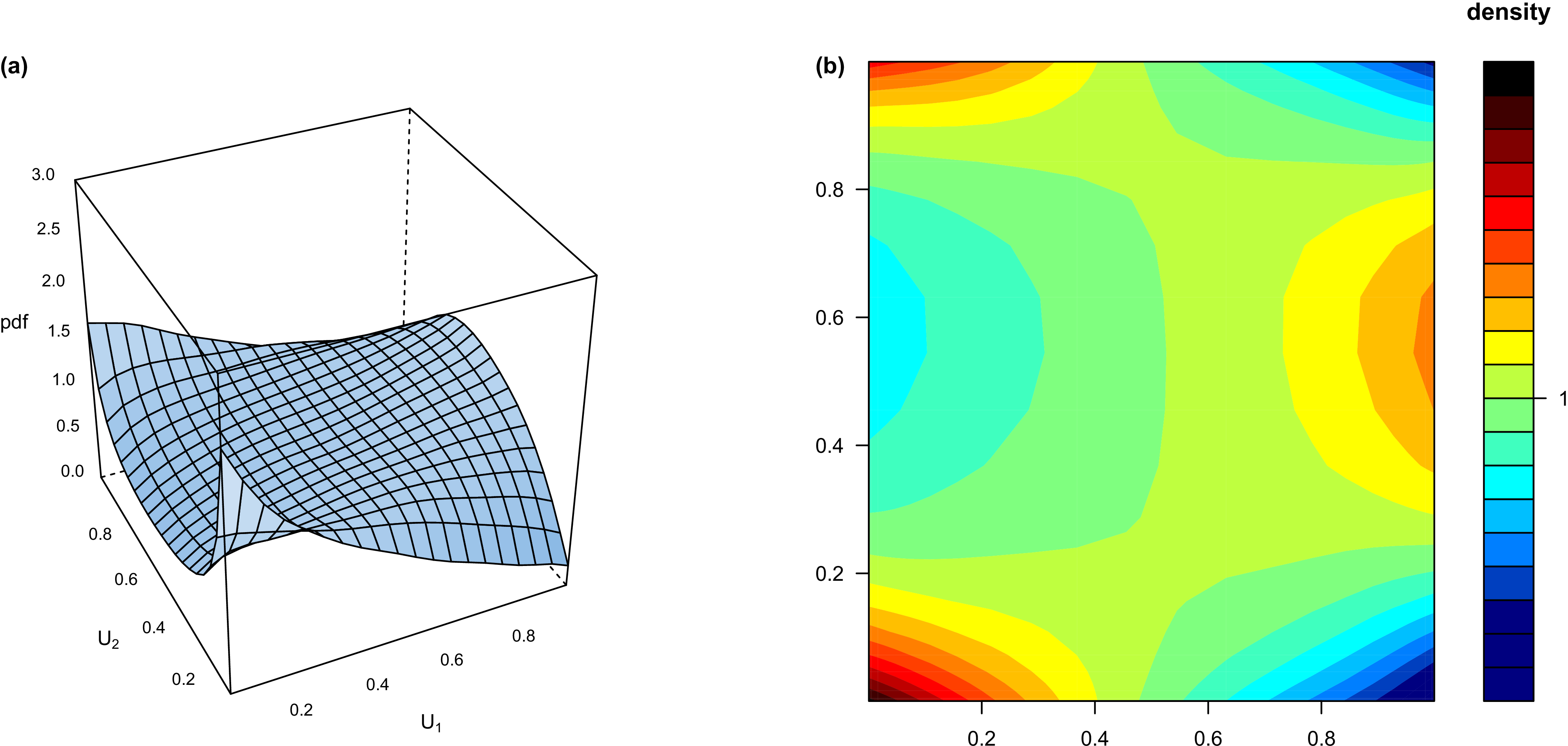
The visualization of the copula density function provided by Oh et al. (Reference Oh, Ahn and Lee2021a) offers valuable insight into the dependence structure. Specifically, Figure 1, adapted from Oh et al. (Reference Oh, Ahn and Lee2021a), illustrates the jittered version of the copula density corresponding to
 $(N^+, M^+)$
in Model 2 with
 ${\mathbb{P}}\left(N^+=n\right)=0.2$
,
 $n=1, 2, 3, 4, 5.$
The jittered version of the copula density corresponding to
 $(N^+, M^+)$
(Oh et al., Reference Oh, Ahn and Lee2021a).

Figure 1. Long description
Panel A: A 3D surface plot shows the probability density function (pdf) of two variables, U1 and U2. The x-axis represents U1, the y-axis represents U2, and the z-axis represents the pdf. The surface plot shows a mesh grid with varying heights, indicating the relationship between U1, U2, and the pdf. Panel B: A 2D contour plot displays the density of the copula corresponding to the collective risk model. The x-axis represents U1, and the y-axis represents U2. The contour plot uses a color gradient to represent different density levels, with a legend on the right side indicating the density values. The colors range from blue (low density) to red (high density), showing the distribution of density across the U1 and U2 space.
Although various copula families, including the Gaussian copula and Archimedean copulas, have been used to model dependence between frequency and average severity in the insurance literature, none of the existing choices can fully explain monotone conditional variance property nor stochastically monotone wing property (Erdemir and Meral, Reference Erdemir and Meral2020; Gao and Li, Reference Gao and Li2023). To address this limitation, we introduce a novel copula family derived from the well-known NG distribution (Jewell, Reference Jewell1974; DeGroot, Reference DeGroot2005; Bernardo and Smith, Reference Bernardo and Smith2009). This new copula family possesses both the monotone conditional variance property and the stochastically monotone wing property, making it a promising candidate for modeling the dependence structure between
 $N^+$
and
 $M^+$
.
3. Introduction to a new family of copulas
This section introduces a new copula family derived from the NG distribution. We begin by defining the NG distribution and reviewing its essential properties.
3.1. Normal-Gamma copula
Model 3. [NG Distribution]. A bivariate random variable (X, Y) follows a NG distribution if
 \begin{equation}Y\,|\, X \sim \textrm{N}\left(0, \frac{1}{X} \right)\quad\text{and}\quad X \sim\textrm{Gamma}\left(\alpha, \beta \right), \end{equation}
where
 $N(\mu, \sigma^2)$
implies a normal distribution with mean
 $\mu\in\mathbb{R}$
and variance
 $\sigma^2\gt 0$
, and
 $\textrm{Gamma}\left(\alpha, \beta \right)$
denotes a gamma distribution with shape parameter
 $\alpha\gt 0$
and rate parameter
 $\beta\gt 0$
.
The NG distribution defined in Model 3 exhibits a well-known conjugate property, as demonstrated in part i of the following corollary. Furthermore, part ii shows that the marginal distributions can be expressed analytically.
Corollary 3.1. For a bivariate random variable (X, Y) as described in Model 3, we have the following properties:
-
(i) The conditional distribution of X given
$Y=y$
is
\[X \,|\, Y=y \sim \textrm{Gamma}\left(\alpha+\frac{1}{2}, \beta +\frac{1}{2}y^2\right).\]
-
(ii) The marginal distribution of Y is
where
\[Y\sim \textrm{t}_{2\alpha}\left(0, \frac{\beta}{\alpha}\right),\]
$\textrm{t}_\nu \left(\mu, \tau^2 \right)$
implies the location-scale Student’s t distribution with degree of freedom parameter
$\nu\gt 0$
, location parameter
$\mu\in\mathbb{R}$
, and scale parameter
$\tau^2\gt 0$
.


The following result provides an expression for the copula family corresponding to the NG distributions presented in Model 3.
Proposition 3.2. For a bivariate random variable (X, Y) as described in Model 3, we obtain the following results:
-
(i) The joint distribution function of (X, Y) at
$(X,Y)=(x,y)$
, denoted by
$H_{\alpha, \beta}\;:\;\mathbb{R}^2\rightarrow [0,1]$
, is given by (5)where
\begin{equation} H_{\alpha, \beta}(x, y)=\int_{-\infty}^{x}\int_{-\infty}^{y}h_{\alpha, \beta}(s, t;\;\alpha, \beta) \,\textrm{d}t\,\textrm{d}s, \end{equation}
$h_{\alpha, \beta}\;:\;\mathbb{R}^2\rightarrow \mathbb{R}_{\ge 0}$
is the corresponding joint density function defined by (6)
\begin{equation} h_{\alpha, \beta}(x,y;\;\alpha, \beta)= \begin{cases} \dfrac{\beta^\alpha}{\Gamma(\alpha)\sqrt{2\pi}} \,x^{\alpha+\dfrac{1}{2}-1}\exp\left( -x\left( \beta+\frac{y^2}{2}\right)\right), & x \in \mathbb{R}_{\gt 0}, \, y \in \mathbb{R};\\[5pt] 0, & \text{otherwise}. \end{cases} \end{equation}
-
(ii) Let
$C_{\alpha, \beta}\in\mathcal{F}_2$
be a bivariate copula corresponding to
$H_{\alpha, \beta}\;:\;\mathbb{R}^2\rightarrow [0,1]$
for some
$\alpha, \beta\gt 0$
. Then, we have (7)where
\begin{equation} C_{\alpha, \beta}(u,v)=\int_{0}^{u}\int_{0}^{v} c_{\alpha, \beta}(s,t) \, \textrm{d}t\,\textrm{d}s, \quad u,v\in[0,1], \end{equation}
$c_{\alpha, \beta}\;:\;[0,1]^2\rightarrow \mathbb{R}_{\ge 0}$
is the corresponding copula density function defined by (8)for
\begin{equation} \begin{aligned} &c_{\alpha, \beta}(u,v) \\ &\quad= \frac{\beta^\alpha}{\Gamma(\alpha)\sqrt{2\pi}}\frac{ \left(G^{-1}\left( u ;\;\alpha, \beta\right) \right)^{\alpha+\frac{1}{2}-1}\exp\left( -G^{-1}\left( u ;\;\alpha, \beta\right) \left( \beta+ \frac{1}{2}\left(\Phi_{2\alpha}^{-1}\left( v ;\;0, \frac{\beta}{\alpha}\right) \right)^2\right)\right) } {g\left( G^{-1}\left( u ;\;\alpha, \beta\right)\!;\;\alpha, \beta\right) \phi_{2\alpha}\left( \Phi_{2\alpha}^{-1}\left( v ;\;0, \frac{\beta}{\alpha}\right)\!;\;0, \frac{\beta}{\alpha}\right) }\\&\quad{=\frac{\beta^\alpha}{\Gamma(\alpha)\sqrt{2\pi}}\frac{\left(G^{-1}\left(u;\;\alpha,\beta\right)\right)^{\alpha+\frac{1}{2}-1}\exp\left[-G^{-1}\left(u;\;\alpha,\beta\right)\left\{\beta+\frac{1}{2}\left(\Phi_{2\alpha}^{-1}\left(v;\;0,\frac{\beta}{\alpha}\right)\right)^2\right\}\right]}{\frac{\beta^\alpha}{\Gamma(\alpha)}\left(G^{-1}\left(u;\;\alpha,\beta\right)\right)^{\alpha-1}\exp\left[-\beta G^{-1}\left(u;\;\alpha,\beta\right)\right]\phi_{2\alpha}\left(\Phi_{2\alpha}^{-1}\left(v;\;0,\frac{\beta}{\alpha}\right)\!;\;0,\frac{\beta}{\alpha}\right)}}\\&\quad=\frac{1}{\sqrt{2\pi}}\frac{ \left(G^{-1}\left( u ;\;\alpha, \beta\right) \right)^{\frac{1}{2}} \exp\left( -\frac{1}{2}G^{-1}\left( u ;\;\alpha, \beta\right) \left(\Phi_{2\alpha}^{-1}\left( v ;\;0, \frac{\beta}{\alpha} \right)\right)^2\right) } { \phi_{2\alpha}\left( \Phi_{2\alpha}^{-1}\left( v ;\;0, \frac{\beta}{\alpha}\right)\!;\;0, \frac{\beta}{\alpha}\right) }, \end{aligned} \end{equation}
$u,v\in(0,1)$
. Here,
$G(\cdot;\; \alpha, \beta)$
and
$g(\cdot;\; \alpha, \beta)$
denote the cumulative distribution function and probability density function of the gamma distribution with shape parameter
$\alpha \gt 0$
and rate parameter
$\beta \gt 0$
, respectively. Similarly,
$\Phi_\nu(\cdot;\; \mu, \tau^2)$
and
$\phi_\nu(\cdot;\; \mu, \tau^2)$
denote the cumulative distribution function and probability density function of the location-scale Student’s t-distribution with degrees of freedom
$\nu \gt 0$
, location parameter
$\mu \in \mathbb{R}$
, and scale parameter
$\tau^2 \gt 0$
, respectively.




Proof. The proof of part i follows directly from Model 3. For part ii, Sklar’s theorem gives
 \[C_{\alpha,\beta}(u,v)=H_{\alpha,\beta}\left(G^{-1}(u;\;\alpha,\beta),\Phi_{2\alpha}^{-1}\left(v;\;0,\frac{\beta}{\alpha}\right)\right).\]
Differentiating this identity with respect to u and v, using Corollary 3.1, gives (8).
While it is not immediately obvious from the expression in (8), the following result demonstrates that the parameter
 $\beta \gt 0$
is redundant in defining the copula in (7) and hence its corresponding density function in (8).
Lemma 3.3. The copula in (8) is invariant with respect to the parameter
 $\beta \gt 0$
.
Proof. Consider the random variable (X, Y) in (4). The copula corresponding to (X, Y) is identical to the copula corresponding to
 $(\beta X, Y)$
because the copula is invariant under the strictly monotone transformation of the random variables, as stated in Theorem 2.4.3 of Nelsen (Reference Nelsen2007). Since
 $\beta X \sim \mathrm{Gamma}(\alpha, 1)$
, the proof is concluded.
Lemma 3.3 implies that we can set
 $\beta = 1$
without loss of generality when defining the copula family corresponding to the NG distribution. Consequently, the copula in (8) depends only on the parameter
 $\alpha \gt 0$
. Furthermore, we found it convenient to use the alternative parameterization
 $\theta = 1/\alpha$
. With
 $\alpha = 1/\theta$
and
 $\beta = 1$
, the joint density function in (6) and the copula density function in (8) can then be expressed as
 \[ h_{\theta}(x,y)\;:\!=\; \begin{cases} \dfrac{1}{\Gamma(\frac{1}{\theta})\sqrt{2\pi}} \,x^{\frac{1}{\theta}-\frac{1}{2}}\exp\left( -x\left( 1+\frac{y^2}{2}\right)\right), & x, y\in\mathbb{R}_{\gt 0}\times\mathbb{R};\\ 0, & \hbox{otherwise}, \end{cases}\]
and
 \begin{equation}\begin{aligned} c_{\theta}(u,v) \;:\!=\;\frac{1}{\sqrt{2\pi} }\frac{\left(G^{-1}\left( u ;\;\frac{1}{\theta}, 1\right) \right)^{1/2} \,\exp\left( -\frac{1}{2}G^{-1}\left( u ;\;\frac{1}{\theta}, 1\right) \left(\Phi_{2/\theta}^{-1}\left( v ;\;0, \theta\right) \right)^2 \right)}{\phi_{2/\theta}\left( \Phi_{2/\theta}^{-1}\left( v ;\;0, \theta\right)\!;\;0, \theta\right)},\end{aligned}\end{equation}
respectively. This copula family is formally defined in Definition 3.4.


3.2. Properties of Normal-Gamma copulas
We first record a symmetry property of the NG copula. Although this property is not the primary modeling motivation in the frequency-severity setting, it plays an important technical role in the sequel and is used repeatedly in the proofs of the main dependence properties. In particular,
 $C_{\theta}(u,v)$
is symmetric with respect to the horizontal line
 \begin{equation}\left\{ (u,v)\in(0,1)^2\,\big|\,v=\frac{1}{2}\right\}.\end{equation}
Lemma 3.5. A NG copula
 $C_{\theta}\in\mathcal{S}$
for some
 $\theta\gt 0$
is symmetric along the horizontal line in (10). Specifically, we have
 \[C_{\theta}(u,v)=u-C_{\theta}(u,1-v), \quad u,v\in(0,1).\]
Proof. It is enough to show
 \begin{equation}c_{\theta}\left(u,\frac{1}{2}-v\right)=c_{\theta}\left(u,\frac{1}{2}+v\right), \quad u\in(0,1) \quad\hbox{and}\quad v\in\left(0,\frac{1}{2}\right).\end{equation}
First, due to the symmetry of the Student’s t distribution, we have
 \[\Phi_{2/\theta}^{-1}\left( \frac{1}{2}-v ;\;0, \theta\right) = -\Phi_{2/\theta}^{-1}\left( \frac{1}{2}+v ;\;0,\theta\right)\]
and
 \[\phi_{2/\theta}\left( \frac{1}{2}-v ;\;0, \theta\right)=\phi_{2/\theta}\left( \frac{1}{2}+v ;\;0, \theta \right)\]
for
 $v\in\left( 0, \frac{1}{2}\right)$
. Applying these results to (9), we have (11).
The NG copula family also satisfies the stochastically monotone wing property, which was proposed in Oh and Ahn (Reference Oh and Ahn2024). We note that the stochastically monotone wing property can be viewed as an extension of the stochastically increasing property proposed by Tukey (Reference Tukey1958) and Lehmann (Reference Lehmann1966). It is shown that this property remains invariant under strictly increasing transformations of the marginal distributions, and hence characterizes the copula itself (Oh and Ahn, Reference Oh and Ahn2024).
Theorem 3.6. For a NG copula
 $C_{\theta}\in\mathcal{S}$
, consider a random vector
 $(U,V)\sim C_{\theta}$
. Then, we have
 \begin{equation}{\mathbb{P}}\left(V\gt\frac{1}{2}+v \,\big\vert\, U=u\right)\end{equation}
and
 \begin{equation*}{\mathbb{P}}\left(V\lt\frac{1}{2}-v \,\big\vert\, U=u\right)\end{equation*}
are decreasing functions of
 $u\in(0,1)$
for all
 $v\in(0,1/2)$
.
Proof. By the symmetry in Lemma 3.5, it is enough to show (12). First, for
 $u\in(0,1)$
and
 $v\in(0, 1/2)$
, we have
 \begin{equation}{\mathbb{P}}\left(V\gt\frac{1}{2}+v \,\big\vert\, U=u\right)=1-\Phi\left(\Phi_{2/\theta}^{-1}\left( \frac{1}{2}+v ;\; 0, \theta\right)\sqrt{G^{-1}\bigg(u;\; \frac{1}{\theta}, 1\bigg)}\right)\end{equation}
by (4) and Corollary 3.1, where
 $\Phi(\!\cdot\!)$
is a cumulative distribution function of standard normal distribution. Since
 \[\Phi_{2/\theta}^{-1}\left( \frac{1}{2}+v ;\; 0, \theta \right)\gt 0\]
for any given
 $v\in(0, 1/2)$
, it is clear that (13) is a decreasing function of
 $u\in(0,1)$
for any given
 $v\in(0, 1/2)$
.
The following result, which is a corollary of Theorem 3.6, shows that the NG copula has the monotone conditional variance property, which was proposed in Oh and Ahn (Reference Oh and Ahn2024).
Theorem 3.7. Consider a NG copula
 $C_{\theta}\in\mathcal{S}$
for some
 $\theta\gt 0$
, and the corresponding bivariate random variable
 $(U,V)\sim C_{\theta}$
. Then, we have the following properties:
-
i.
${\mathbb E}\left[V \,|\, U=u\right]=\frac{1}{2}$
for
$u\in(0,1)$
. -
ii.
${\mathrm Var}\left(V \,|\, U=u\right)$
is a decreasing function of u on the open interval (0, 1).


Proof. The proof of part i follows immediately from the symmetry of the copula in Lemma 3.5. Now, we prove part ii. For
 $u\in(0,1)$
, we have
 \[\begin{aligned}{\mathrm Var}\left(V\,|\, U=u\right)&={\mathbb E}\left[\left( V-\frac{1}{2}\right)^2 \,\big\vert\, U=u\right]\\&=4\int\limits_{0}^{\frac{1}{2}}v{\mathbb{P}}\left(V\gt\frac{1}{2}+v\,\big\vert\, U=u\right) \textrm{d} v,\end{aligned}\]
where the first equality is from part i, and the second equality is from Lemma 3.5 and integration by parts. Then, combining this result with Theorem 3.6, we conclude the proof.
Note that the decreasing conditional variance property is also affected by the value of
 $\theta$
. For example, in the case of
 $\theta \rightarrow 0$
, the copula
 $C_\theta(u,v)$
approaches to an independence copula as described in Theorem 3.8 so that
 $\lim_{\theta \rightarrow 0}{\mathrm Var}\left(V|U=u\right)={\mathrm Var}\left(V\right)=1/12$
. On the other hand, in the case of
 $\theta \rightarrow \infty$
, one can observe that
 $U=1-|2V-1|$
for
 $U \in (0,1)$
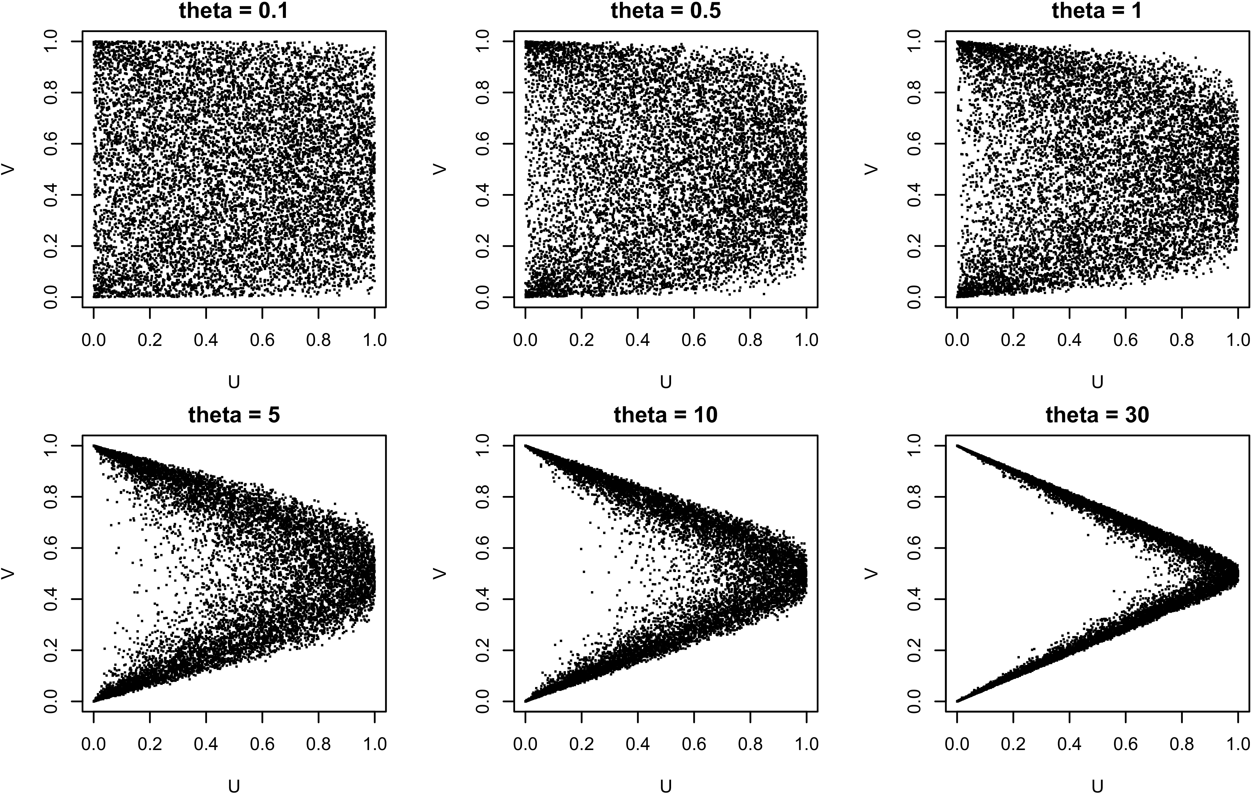
from Figure 2 so that
 $\lim_{\theta \rightarrow \infty}{\mathrm Var}\left(V|U=u\right)=0.5 \cdot (1-0.5u - 0.5)^2 + 0.5 \cdot (0.5u - 0.5)^2=0.25 (u-1)^2$
for
 $u \in (0,1)$
.
Scatterplots of 10,000 samples of (U, V) under the NG copula with
 $\theta=(0.1, 0.5,1,5, 10, 30)$
.

3.3. Limiting behavior of Normal–Gamma copula
In Figure 2, we display scatterplots of random samples generated from the NG copula
 $C_\theta$
for several values of
 $\theta \gt 0$
. As
 $\theta$
decreases toward zero, the samples exhibit progressively weaker dependence, converging to the pattern of an independence copula. Conversely, as the copula parameter
 $\theta$
tends to infinity, the dependence structure induced by the NG copula converges to a degenerate copula whose probability mass is entirely concentrated on the set
 \begin{equation}\{(u,v)\in (0,1)^2\;:\; u=1-|2v-1|\}.\end{equation}
This section provides the rigorous statements for two asymptotic behaviors of the NG copula; one when
 $\theta\searrow 0$
and the other
 $\theta\rightarrow \infty$
. We start with the asymptotic behavior of the NG copula as
 $\theta$
goes to zero. The proof is given in Appendix B.
Theorem 3.8. For
 $(u,v)\in(0,1)^2$
, we have
 \begin{equation*} \lim\limits_{\theta \searrow 0}c_{\theta}(u,v) =1.\end{equation*}
Now, as
 $\theta\to\infty$
, we establish that the NG copula converges to a degenerate copula whose probability mass is entirely concentrated on the set in (14). Equivalently, for
 $(U, V) \sim C_\theta$
, this implies that (U, V) are countermonotonic given
 $V\gt 1/2$
and comonotonic given
 $V\lt 1/2$
; see Theorem 3.9 for the formal statement. The proof is given in Appendix C.
Theorem 3.9. Let
 $(U_i, V_i)$
,
 $i=1,2$
, be independent copies drawn from the NG copula
 $C_\theta$
. Then, as
 $\theta\to\infty$
, we have
-
i. Countermonotonicity in the upper half
\[ \lim_{\theta\rightarrow\infty} {\mathbb{P}}((V_2 - V_1)(U_2-U_1) \lt 0 \,|\, V_1\gt 1/2,\; V_2\gt 1/2) = 1. \]
-
ii. Comonotonicity in the lower half
\[ \lim_{\theta\rightarrow\infty} {\mathbb{P}}( (V_2 - V_1)(U_2-U_1) \gt 0 \,|\, V_1\lt 1/2,\; V_2\lt 1/2) = 1. \]


4. Application to the collective risk model
This section presents the CRM, where the NG copula
 $C_\theta\in\mathcal{S}$
is used to model the dependence between the frequency and the average severity. We start with special case of the positive CRM in Model 1.
Model 4. Consider the setting in Model 1 where a copula
 $C\in\mathcal{F}_2$
is modeled by an NG copula
 $C_\theta\in\mathcal{S}$
.
Now, we derive the following analytical result on the conditional distribution, which is the key result to calculate the Radon–Nikodym derivative of the distribution of
 $(N^+,M^+)$
defined in (2). Although conditioning on severity given frequency is more common in collective risk modeling, we consider the reverse conditioning here as a technical step that enables an explicit characterization of the joint density of
 $(N^+,M^+)$
.
Lemma 4.1. Consider the setting in Model 1. Then, we have
 \begin{align*}{\mathbb{P}}(N^+ &= n \,|\, M^+ = m)\\& = G\left( G^{-1}\left( F_1^+(n);\; \frac{1}{\theta}, 1 \right)\!;\; \frac{1}{\theta}+\frac{1}{2},\, 1+\frac{1}{2}\left( \Phi_{2/\theta}^{-1}\left( F_2^+(m);\; 0, \theta\right) \right)^2 \right)\\&\quad -G\left( G^{-1}\left( F_1^+(n-1); \frac{1}{\theta}, 1 \right)\!;\; \frac{1}{\theta}+\frac{1}{2},\, 1+\frac{1}{2}\left( \Phi_{2/\theta}^{-1}\left( F_2^+(m);\; 0, \theta\right) \right)^2 \right)\end{align*}
for
 $m\in\mathbb{R}_{\gt 0}$
and
 $n\in\mathbb{N}_{\gt 0}$
.
Proof. For
 $N^+\sim F_1^+$
, consider
 \[N^*\;:\!=\;N^+-U,\]
where
 $U\sim \textrm{Unif}(0,1)$
, and
 $N^+$
and U are independent. Then, if we let
 $F_1^*$
be a cumulative distribution function of
 $N^*$
, we have
 \[F_1^*(n)=F_1^+(n), \quad n\in\mathbb{N}_{\gt 0}\]
and
 \[F_1^*(N^+-U)\sim \textrm{Unif}(0,1).\]
Then, for
 $C_{\theta}\in\mathcal{S}$
with some
 $\theta\gt 0$
, consider
 \[(N^*, M^+)\sim C_{\theta}\left(F_1^*, F_2^+ \right).\]
Since both
 $F_1^*$
and
 $F_2^+$
are absolutely continuous cumulative distribution functions, we have
 \[\left( F_1^*(N^*), F_2^+(M^+)\right) \sim C_{\theta}\]
and
 \[\left(G^{-1}\left( F_1^*(N^*);\; \frac{1}{\theta}, 1 \right), \Phi_{2/\theta}^{-1}\left( F_2^+(M^+);\; 0, \theta\right) \right)\sim H_{\theta},\]
where
 $H_{\theta}$
is the joint distribution of the NG distribution defined in (5), and
 $C_{\theta}$
is the corresponding copula function defined in (7). Then, Corollary 3.1 yields
 \[\begin{aligned}&{\mathbb{P}}\left(N^+\le n \,|\, M^+=m\right)\\&={\mathbb{P}}\left(N^*\le n \,|\, M^+=m\right)\\&={\mathbb{P}}\left( G^{-1}\left( F_1^*(N^*);\; \frac{1}{\theta},1 \right)\le G^{-1}\left( F_1^*(n);\; \frac{1}{\theta}, 1 \right) \Big| \Phi_{2/\theta}^{-1}\left( F_2^+(M^+);\; 0, \theta\right)=\Phi_{2/\theta}^{-1}\left( F_2^+(m);\; 0, \theta\right)\right)\\&=G\left( G^{-1}\left( F_1^*(n);\; \frac{1}{\theta}, 1 \right)\!;\; \frac{1}{\theta}+\frac{1}{2},\, 1+\frac{1}{2}\left( \Phi_{2/\theta}^{-1}\left( F_2^+(m);\; 0, \theta\right)\right)^2\right)\\&=G\left( G^{-1}\left( F_1^+(n);\; \frac{1}{\theta}, 1 \right)\!;\; \frac{1}{\theta}+\frac{1}{2},\, 1+\frac{1}{2}\left( \Phi_{2/\theta}^{-1}\left( F_2^+(m);\; 0, \theta\right)\right)^2\right) \end{aligned}\]
for
 $m\in\mathbb{R}_{\gt 0}$
and
 $n\in\mathbb{N}_{\gt 0}$
. This concludes the proof.
Since Model 1 assumes positive frequency, it cannot be directly applied to real-world data that includes zero frequencies. In the following, we present a modified version of Model 1, which accommodates zero frequency.
Model 5. (General CRM). Consider the setting described in Model 4. Given a constant
 $p \in (0,1)$
and a random variable
 $R \sim \text{Ber}(p)$
, where
 $\text{Ber}(p)$
denotes the Bernoulli distribution with parameter p, and R is independent of
 $(N^+, M^+)$
, we define
 \[N \;:\!=\; R \, N^+ \quad \hbox{and} \quad M \;:\!=\; R \, M^+.\]
We refer to N as the frequency and M the average severity. The corresponding joint density function
 $h\;:\; \mathbb{N}_{\ge 0}\times \mathbb{R}_{\ge 0}\rightarrow \mathbb{R}_{\ge 0}$
is defined as the Radon–Nikodym derivative of the distribution of (N, M) with respect to the product of the counting measure on
 $\mathbb{N}_{\ge 0}$
and Lebesgue measures on
 $\mathbb{R}_{\ge 0}$
:
 \begin{equation}\begin{aligned}h(n, m)&\;:\!=\; \frac{\partial}{\partial\, m}\left( {\mathbb{P}}\left(N\le n, \, M\le m\right)-{\mathbb{P}}\left(N\le n-1, \, M\le m\right)\right)\\\end{aligned}\end{equation}
for
 $n\in\mathbb{N}_{\ge 0},\, m\in\mathbb{R}_{\ge 0}$
.
The following corollary is a direct result of Model 5.
Corollary 4.2. Under the settings in Model 15, the Radon–Nikodym derivative of the distribution of (N, M) in (15) is obtained by
 \[h(n,m)=\begin{cases}1-p, & n=0 \quad\hbox{and}\quad m=0;\\p\, h^+(n,m), & n\in\mathbb{N}_{\gt 0} \quad\hbox{and}\quad m\gt 0;\\0, &\hbox{otherwise.}\\\end{cases}\]

Remark 1. Although a copula can in principle be applied directly to the mixed pair (N, M), we separate the zero-claim and positive-claim regimes. The reason is that (0, 0) is a structural point: when
 $N=0$
, the average severity is not observed and is set equal to zero by convention. Hence, if
 $p=\mathbb{P}(N\gt 0)$
, then a copula fitted directly to (N, M) would have to allocate probability mass
 $\mathbb{P}(N=0,M=0)=1-p$
to the lower-left structural zero component. Thus, when zero-claim observations form a large portion of the portfolio, as is common in auto insurance portfolios, a substantial part of the copula probability mass on
 $[0,1]\times[0,1]$
is used to represent this deterministic zero-zero association. Only the remaining probability mass p is available to describe the actual dependence between frequency and average severity among policies with positive claims. Our Bernoulli construction separates the claim-occurrence mechanism from the positive-claim dependence structure and applies the NG copula fully devoted to
 $(N^+,M^+)$
, where average severity is genuinely observed and the dependence of interest is modeled directly by the copula.
5. Numerical study
5.1. Finite sample property
We conduct a simulation study to investigate the finite sample properties of the parameter estimation and the dependence between frequency and the average severity based on Model 5. To accommodate the realistic setting, we consider
 $\mathbf{x}$
as a row vector of the explanatory variables, and the column vectors
 $\beta_1$
and
 $\beta_2$
are corresponding sets of regression coefficients for the frequency and severity parts, respectively. We also consider the exposure w of each policy. Then, for given
 $\mathbf{x}$
and w, we consider
 $R\,|\, \mathbf{x}, w\sim \textrm{Ber}(p)$
and
 $N^+\,|\, \mathbf{x}, w\sim F_1^+$
such that we have
 \begin{equation} N\,|\, \mathbf{x}, w\sim \text{NB}( \lambda w, rw) \quad \text{with} \quad \lambda=\exp\!(\mathbf{x}\beta_1),\end{equation}
where
 $N \sim \text{NB}(\mu, s)$
implies the negative binomial distribution with
 ${\mathbb E}\left[N\right]=\mu$
and
 ${\mathrm Var}\left(N\right)=\mu+\mu^2 / s $
. Specifically, we set
 $ p=1-{\mathbb{P}}\left(N=0\,|\, \mathbf{x}, w\right)$
and
 \[{\mathbb{P}}\left(N^+=n\,|\, \mathbf{x}, w\right)=\frac{{\mathbb{P}}\left(N=n\,|\, \mathbf{x}, w\right)}{p}, \quad n\in\mathbb{N}_{\gt 0}.\]
For the marginal distribution of the positive average severity, we assume generalized beta of the second kind (GB2) distribution,
 \begin{equation} M^+ | \mathbf{x}, w \sim \text{GB2}(1,\xi, w\psi, wk+1) \quad \text{with} \quad \xi = \exp\!(\mathbf{x}\beta_2),\end{equation}
with
 \[{\mathbb E}\left[M^+\mid \mathbf{x}, w\right]=\xi\frac{\psi}{k},\]
and, whenever the second moment exists,
 $wk\gt 1$
,
 \[{\mathrm Var}\left(M^+\mid \mathbf{x}, w\right)=\xi^2\frac{\psi(\psi+k)}{k^2(wk-1)}.\]
where
 $\text{GB2}(a,b, p, q)$
indicates that GB2 distribution with scale parameter
 $b\gt 0$
and shape parameters
 $a, p, q \gt 0$
and its probability density function is given by
 \[ g(s;\; a,b,p,q)= \frac{a(s/b)^{ap-1}}{b B(p,q) (1+(s/b)^a)^{p+q}}.\]
Note that the motivation of the using the exposure in (17) is in Remark 2.
Remark 2. For the frequency component, the exposure specification in (16) is standard, and in this case, both
 \[{\mathbb E}\left[N\mid \mathbf{x}, w\right]=\lambda w\quad\hbox{and}\quad{\mathrm Var}\left(N\mid \mathbf{x}, w\right)=\lambda w+\frac{\lambda^2}{r}w,\]
are of order w.
By contrast, there is no equally canonical way to incorporate exposure into the positive average severity. To motivate our specification, suppose that the distribution of the individual severity does not depend on w and define
 \[S^+\;:\!=\;\sum_{j=1}^{N^+} Z_j\quad\hbox{and}\quad M^+\;:\!=\;\frac{S^+}{N^+},\]
as in Model 2. Under the benchmark assumption that
 $N^+$
is independent of the individual severities and that the
 $Z_j$
’s are i.i.d., we have
 \[{\mathbb E}\left[M^+\mid \mathbf{x}, w\right]={\mathbb E}\left[Z_j\mid \mathbf{x}\right],\]
and
 \begin{equation*}{\mathrm Var}\left(M^+\mid \mathbf{x}, w\right)={\mathrm Var}\left(Z_j\mid \mathbf{x}\right){\mathbb E}\left[\frac{1}{N^+}\,\bigg|\, \mathbf{x}, w\right].\end{equation*}
Hence, even in this simplest benchmark model, the mean of
 $M^+$
is invariant to the exposure, while its variance decreases with w through the term
 \[{\mathbb E}\left[\frac{1}{N^+}\,\bigg|\, \mathbf{x}, w\right].\]
Moreover, outside the independence setting, the exact form of this exposure effect depends on the dependence structure between frequency and severity. For this reason, instead of imposing an offset structure analogous to that of the frequency model, we adopt the GB2 specification in (17), which preserves an exposure-invariant mean while allowing the variance to decrease flexibly with w through the additional parameter
 $k\gt 0$
.
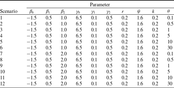
A portfolio of 5000 policyholders (
 $I=5000$
) is generated from the proposed model under 12 scenarios motivated by the real data analysis in Section 6. Table 1 provides the parameter settings. Each simulation uses two categorical variables,
 $x_1$
and
 $x_2$
, generated independently from
 $\text{Ber}(0.5)$
; hence, we have
 $\mathbf{x}=[1,\, x_1,\, x_2]$
.
Parameter settings for the 12 scenarios.

Table 1. Long description
A table with 12 rows and 10 columns. The columns are labeled as Scenario, beta 0, beta 1, beta 2, gamma 0, gamma 1, gamma 2, r, psi, k, and theta. Each row represents a different scenario with specific parameter settings. Row 1: Scenario 1, beta 0 -1.5, beta 1 0.5, beta 2 1.0, gamma 0 6.5, gamma 1 0.1, gamma 2 0.5, r 0.2, psi 1.6, k 0.2, theta 0.1. Row 2: Scenario 2, beta 0 -1.5, beta 1 0.5, beta 2 1.0, gamma 0 6.5, gamma 1 0.1, gamma 2 0.5, r 0.2, psi 1.6, k 0.2, theta 0.5. Row 3: Scenario 3, beta 0 -1.5, beta 1 0.5, beta 2 1.0, gamma 0 6.5, gamma 1 0.1, gamma 2 0.5, r 0.2, psi 1.6, k 0.2, theta 1. Row 4: Scenario 4, beta 0 -1.5, beta 1 0.5, beta 2 1.0, gamma 0 6.5, gamma 1 0.1, gamma 2 0.5, r 0.2, psi 1.6, k 0.2, theta 5. Row 5: Scenario 5, beta 0 -1.5, beta 1 0.5, beta 2 1.0, gamma 0 6.5, gamma 1 0.1, gamma 2 0.5, r 0.2, psi 1.6, k 0.2, theta 10. Row 6: Scenario 6, beta 0 -1.5, beta 1 0.5, beta 2 1.0, gamma 0 6.5, gamma 1 0.1, gamma 2 0.5, r 0.2, psi 1.6, k 0.2, theta 30. Row 7: Scenario 7, beta 0 -1.5, beta 1 0.5, beta 2 2.0, gamma 0 6.5, gamma 1 0.1, gamma 2 0.5, r 0.2, psi 1.6, k 0.2, theta 0.1. Row 8: Scenario 8, beta 0 -1.5, beta 1 0.5, beta 2 2.0, gamma 0 6.5, gamma 1 0.1, gamma 2 0.5, r 0.2, psi 1.6, k 0.2, theta 0.5. Row 9: Scenario 9, beta 0 -1.5, beta 1 0.5, beta 2 2.0, gamma 0 6.5, gamma 1 0.1, gamma 2 0.5, r 0.2, psi 1.6, k 0.2, theta 1. Row 10: Scenario 10, beta 0 -1.5, beta 1 0.5, beta 2 2.0, gamma 0 6.5, gamma 1 0.1, gamma 2 0.5, r 0.2, psi 1.6, k 0.2, theta 5. Row 11: Scenario 11, beta 0 -1.5, beta 1 0.5, beta 2 2.0, gamma 0 6.5, gamma 1 0.1, gamma 2 0.5, r 0.2, psi 1.6, k 0.2, theta 10. Row 12: Scenario 12, beta 0 -1.5, beta 1 0.5, beta 2 2.0, gamma 0 6.5, gamma 1 0.1, gamma 2 0.5, r 0.2, psi 1.6, k 0.2, theta 30.
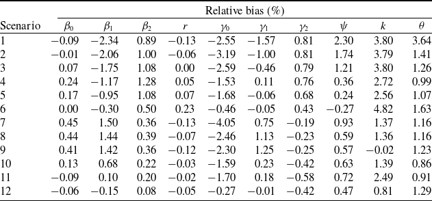
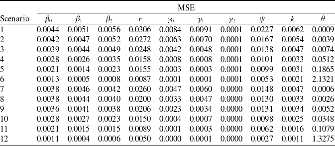
For each scenario, Tables 2 and 3 summarize the simulation results from 100 independent Monte Carlo sample generations. The tables report the relative bias and mean squared error (MSE) of the parameter estimates. Table 2 demonstrates that the estimates in all scenarios closely align with the true model parameters, exhibiting small relative bias and MSE. While Table 3 indicates relatively larger MSE values for
 $\theta=30$
in Scenarios 6 and 12, Table 2 confirms that the corresponding relative biases remain well-controlled.
Relative bias in
 $\%$
for all the parameters from the 12 scenarios.

Table 2. Long description
A table with 12 rows and 8 columns. The columns are labeled as Scenario, β0, β1, β2, r, γ0, γ1, γ2, ψ, k, and θ. Each row represents a different scenario with corresponding values for each parameter. Row 1: Scenario 1, β0 -0.09, β1 -2.34, β2 0.89, r -0.13, γ0 -2.55, γ1 -1.57, γ2 0.81, ψ 2.30, k 3.80, θ 3.64. Row 2: Scenario 2, β0 -0.01, β1 -2.06, β2 1.00, r -0.06, γ0 -3.19, γ1 -1.00, γ2 0.81, ψ 1.74, k 3.79, θ 1.41. Row 3: Scenario 3, β0 0.07, β1 -1.75, β2 1.08, r 0.00, γ0 -2.59, γ1 -0.46, γ2 0.79, ψ 1.21, k 3.80, θ 1.26. Row 4: Scenario 4, β0 0.24, β1 -1.17, β2 1.28, r 0.05, γ0 -1.53, γ1 0.11, γ2 0.76, ψ 0.36, k 2.72, θ 0.99. Row 5: Scenario 5, β0 0.17, β1 -0.95, β2 1.08, r 0.07, γ0 -1.68, γ1 -0.06, γ2 0.68, ψ 0.24, k 2.56, θ 1.07. Row 6: Scenario 6, β0 0.00, β1 -0.30, β2 0.50, r 0.23, γ0 -0.46, γ1 -0.05, γ2 0.43, ψ -0.27, k 4.82, θ 1.63. Row 7: Scenario 7, β0 0.45, β1 1.50, β2 0.36, r -0.13, γ0 -4.05, γ1 0.75, γ2 -0.19, ψ 0.93, k 1.37, θ 1.16. Row 8: Scenario 8, β0 0.44, β1 1.44, β2 0.39, r -0.07, γ0 -2.46, γ1 1.13, γ2 -0.23, ψ 0.59, k 1.36, θ 1.16. Row 9: Scenario 9, β0 0.41, β1 1.42, β2 0.36, r -0.12, γ0 -2.30, γ1 1.25, γ2 -0.25, ψ 0.57, k 1.23. Row 10: Scenario 10, β0 0.13, β1 0.68, β2 0.22, r -0.03, γ0 -1.59, γ1 0.23, γ2 -0.42, ψ 0.63, k 1.39, θ 0.86. Row 11: Scenario 11, β0 -0.09, β1 0.10, β2 0.20, r -0.02, γ0 -1.70, γ1 0.18, γ2 -0.58, ψ 0.72, k 2.49, θ 0.91. Row 12: Scenario 12, β0 -0.06, β1 -0.15, β2 0.08, r -0.05, γ0 -0.27, γ1 -0.01, γ2 -0.42, ψ 0.47, k 0.81, θ 1.29.
Mean squared error for all the parameters from the 12 scenarios.

Table 3. Long description
A table titled ’Mean squared error for all the parameters from the 12 scenarios’ with 12 rows and 11 columns. The columns are labeled as Scenario, beta_0, beta_1, beta_2, r, gamma_0, gamma_1, gamma_2, psi, k, and theta. Each row corresponds to a different scenario and lists the mean squared error values for each parameter. Row 1: Scenario 1, beta_0 0.0044, beta_1 0.0051, beta_2 0.0056, r 0.0306, gamma_0 0.0084, gamma_1 0.0091, gamma_2 0.0001, psi 0.0227, k 0.0062, theta 0.0009. Row 2: Scenario 2, beta_0 0.0042, beta_1 0.0047, beta_2 0.0052, r 0.0272, gamma_0 0.0063, gamma_1 0.0070, gamma_2 0.0001, psi 0.0167, k 0.0054, theta 0.0039. Row 3: Scenario 3, beta_0 0.0039, beta_1 0.0044, beta_2 0.0049, r 0.0248, gamma_0 0.0042, gamma_1 0.0048, gamma_2 0.0001, psi 0.0138, k 0.0047, theta 0.0074. Row 4: Scenario 4, beta_0 0.0028, beta_1 0.0026, beta_2 0.0035, r 0.0158, gamma_0 0.0008, gamma_1 0.0008, gamma_2 0.0001, psi 0.0101, k 0.0033, theta 0.0512. Row 5: Scenario 5, beta_0 0.0021, beta_1 0.0014, beta_2 0.0023, r 0.0155, gamma_0 0.0003, gamma_1 0.0003, gamma_2 0.0001, psi 0.0099, k 0.0031, theta 0.1865. Row 6: Scenario 6, beta_0 0.0013, beta_1 0.0005, beta_2 0.0008, r 0.0087, gamma_0 0.0001, gamma_1 0.0001, gamma_2 0.0001, psi 0.0053, k 0.0021, theta 2.1321. Row 7: Scenario 7, beta_0 0.0038, beta_1 0.0046, beta_2 0.0042, r 0.0260, gamma_0 0.0047, gamma_1 0.0060, gamma_2 0.0000, psi 0.0148, k 0.0047, theta 0.0006. Row 8: Scenario 8, beta_0 0.0038, beta_1 0.0044, beta_2 0.0040, r 0.0200, gamma_0 0.0033, gamma_1 0.0047, gamma_2 0.0000, psi 0.0130, k 0.0033, theta 0.0026. Row 9: Scenario 9, beta_0 0.0036, beta_1 0.0041, beta_2 0.0038, r 0.0206, gamma_0 0.0023, gamma_1 0.0034, gamma_2 0.0000, psi 0.0131, k 0.0034, theta 0.0052. Row 10: Scenario 10, beta_0 0.0028, beta_1 0.0027, beta_2 0.0023, r 0.0150, gamma_0 0.0004, gamma_1 0.0007, gamma_2 0.0000, psi 0.0098, k 0.0025, theta 0.0348. Row 11: Scenario 11, beta_0 0.0021, beta_1 0.0015, beta_2 0.0015, r 0.0089, gamma_0 0.0001, gamma_1 0.0003, gamma_2 0.0000, psi 0.0062, k 0.0016, theta 0.1079. Row 12: Scenario 12, beta_0 0.0011, beta_1 0.0004, beta_2 0.0006, r 0.0050, gamma_0 0.0000, gamma_1 0.0001, gamma_2 0.0000, psi 0.0027, k 0.0011, theta 1.3275.
5.2. Variance and thickness of tail
We now investigate how the variance and right-tail behavior of the predictive distribution of total aggregate loss,
 $\sum_{i=1}^I S_i$
, are affected by the NG copula parameter
 $\theta$
. Recall that a larger
 $\theta$
indicates a stronger decreasing conditional variance property. This could lead to less variation in M given a larger N, potentially resulting in reduced variance and a lighter right tail for the distribution of S as
 $\theta$
increases.
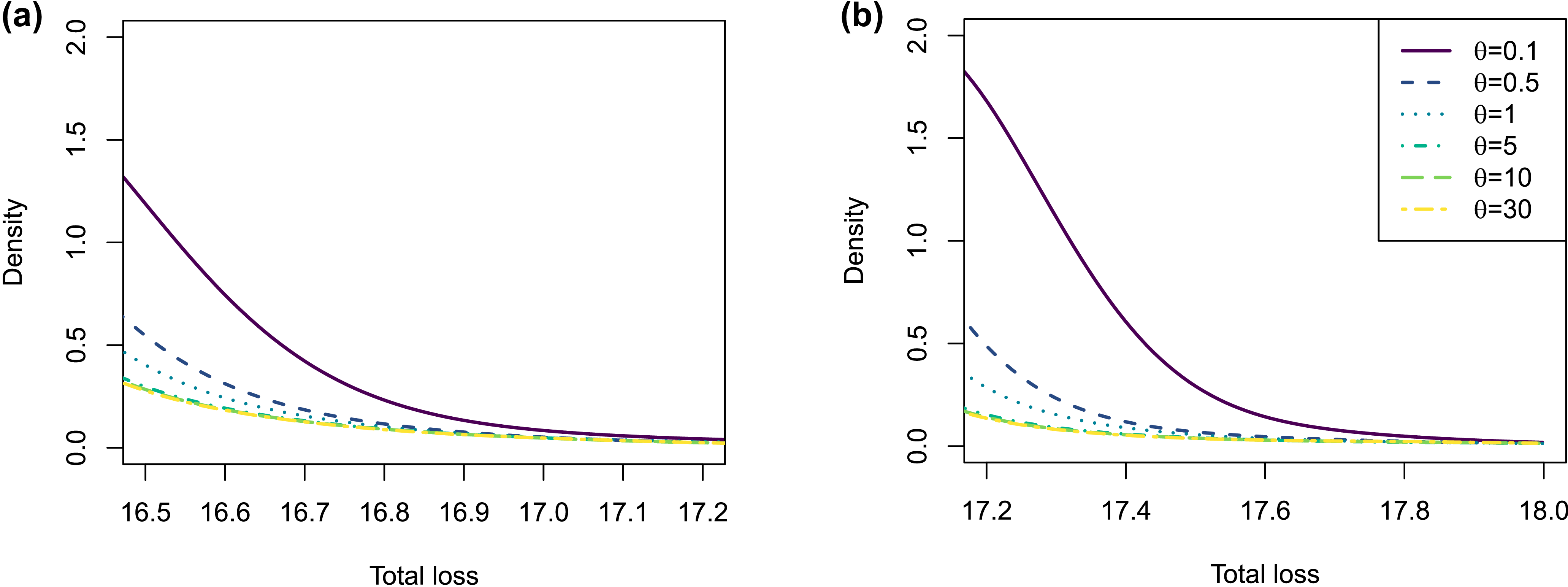
Figure 3 clearly illustrates this phenomenon. It displays the right tail of the predictive distribution of total aggregate loss based on 5000 simulations for each scenario in Table 1. In the left panel, Scenarios 1–6 have identical parameters for the marginal distributions of frequency and average severity. We observe that as
 $\theta$
increases, the right tail of the total aggregate loss distribution becomes lighter. The same trend is evident in the right panel of Figure 3 for Scenarios 7–12.
Right tail of the predictive distribution for the logarithm of the total aggregated losses under (a) Scenarios 1–6 and (b) Scenarios 7–12.

6. Real data analysis
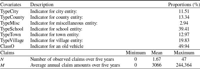
We applied our model to the LGPIF dataset (Frees et al., Reference Frees, Lee and Yang2016), a common benchmark in the actuarial literature (Shi and Lee, Reference Shi and Lee2022; Jeong et al., Reference Jeong, Tzougas and Fung2023). We focused on instances with positive exposure in CO and CN claims, combining five years (2006–2010) of training data using the policy number for merging. We treated the categorical variables O and N as binary covariates. After preprocessing, the dataset contained 817 observations, 329 of which had positive claims. Table 4 summarizes the policy characteristics and claims. The dataset includes a categorical variable representing entity location (City, County, Miscellaneous, School, Town, and Village). We encoded this as five binary indicators (City, County, School, Town, and Village), using Miscellaneous as the reference category. In the real data analysis, we adopt a simplifying assumption that the copula dependence structure is covariate-invariant. This assumption does not affect the MCV property established above, as the result follows from the structural properties of the proposed copula and the marginal specifications, irrespective of whether the dependence parameter is constant or covariate-dependent. Allowing covariate-dependent dependence may increase model flexibility but does not alter the theoretical validity of the MCV property.
Observable policy characteristics and claims information.

Table 4. Long description
A table with 8 rows and 4 columns. The columns are Covariates, Description, Proportions (percent), and Claims. The Covariates column includes TypeCity, TypeCounty, TypeMisc, TypeSchool, TypeTown, TypeVillage, and ClassO. The Description column provides indicators for each covariate. The Proportions (percent) column lists values for each covariate: 11.51 for TypeCity, 13.34 for TypeCounty, 2.94 for TypeMisc, 39.41 for TypeSchool, 12.97 for TypeTown, 19.83 for TypeVillage, and 49.94 for ClassO. The Claims section includes N and M with their descriptions and values: N has a minimum of 0, a mean of 1.67, and a maximum of 47; M has a minimum of 0, a mean of 3066, and a maximum of 244364.
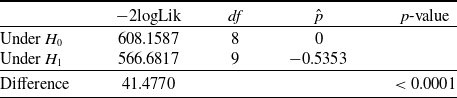
LRT for influence of
 $N^+$
to the dispersion of
 $M^+$
.

Table 5. Long description
A table comparing statistical values under different hypotheses. The table has three rows and four columns. The columns are labeled as -2logLik, df, p-hat, and p-value. The rows are labeled as Under H0, Under H1, and Difference. Row 1: -2logLik, 608.1587; df, 8; p-hat, 0; p-value, blank. Row 2: -2logLik, 566.6817; df, 9; p-hat, -0.5353; p-value, blank. Row 3: Difference, 41.4770; df, blank; p-hat, blank; p-value, <0.0001.
Estimated coefficients and goodness-of-fit of the bivariate copula models.

Table 6. Long description
The table presents estimated coefficients and goodness-of-fit metrics for four different bivariate copula models: Independent, Gaussian copula, Joe copula, and NG copula. It is organized into three main parts: Frequency part, Severity part, and Copula part, each with their respective estimates and standard errors. The table has 25 rows and 12 columns. Column headers include Estimate and Std.err for each model. Row labels include variables such as (Intercept), TypeCity, TypeCounty, TypeSchool, TypeTown, TypeVillage, ClassO, r, ψ, k, and θ. Notable trends include varying estimates and standard errors across different models and parts. The goodness-of-fit section at the bottom includes Loglik, AIC, and BIC values for each model.
Before the dataset is analyzed based on the proposed framework, here we provide another preliminary analysis to detect possible influence of the positive claim frequency (
 $N^+$
) on the conditional variance of
 $M^+$
. To be precise, we want to test the following hypothesis:
 $$\begin{aligned}H_0\;:\;& \text{ Dispersion of $M^+$ conditioned on $N^+$ is not affected by $N^+$}; \\H_1\;:\;& \text{ Dispersion of $M^+$ conditioned on $N^+$ is affected by $N^+$.} \\\end{aligned}$$
To formalize this idea, we adopt an assumption that
 $M^+|N^+$
follows a gamma distribution where
 ${\mathbb E}\left[M^+|N^+\right]=\mu=\exp\!(\mathbf{x}\beta)$
and
 ${\mathrm Var}\left(M^+|N^+\right)=\mu^2 \cdot \psi \cdot (N^+)^p$
. Here, we stick to a gamma distribution only for inference purpose to capture the effect of
 $N^+$
on the dispersion of
 $M^+$
. For example, if we use a GB2 distribution (which has indeed better fit for the severity part of the dataset), then the dispersion is already determined by two shape parameters so it is not intuitive to incorporate the impact of
 $N^+$
in that case. By doing so, the above hypothesis testing can simply be written as
 \[ \begin{aligned}H_0\;:\; p=0 \quad \text{ vs } \quad H_1\;:\; p \ne 0.\end{aligned} \]
Table 5 summarizes the goodness-of-fits for the reduced dispersion model (fitted under
 $H_0$
) and the full dispersion model (fitted under
 $H_1$
). Note that the degree of freedom for the full dispersion model is 9 as it has seven covariates including the intercept for the mean part, and two covariates (intercept and
 $N^+$
) for the dispersion part. From the table, it is shown that the observed dispersion of
 $M^+$
from the dataset is severely impacted by
 $N^+$
, and it is decreasing as
 $N^+$
increases (from the sign of
 $\hat{p}$
,
 $-0.5353$
).
We refer to the proposed model (Model 5), incorporating the marginal models from Section 5, as the NG copula model. For comparison, we also consider various alternative models that utilize different copula components while retaining the same marginals from Section 5, negative binomial for
 $N^+$
as in (16) and GB2 for
 $M^+$
as in (17). Note that appropriateness of GB2 distribution to model the claim severity with the LGPIF data is supported by existing actuarial literature. For a comprehensive model selection procedure, we refer the reader to Frees et al. (Reference Frees, Lee and Yang2016). We compare the following alternative specifications for the copula component of Model 5, assuming identical marginal models. Independent model: This model assumes independence between
 $N^+$
and
 $M^+$
; Gaussian copula model: This model captures dependence using a bivariate Gaussian copula (
 $\theta \in (\!-\!1,1)$
). Note that
 $\theta = 0$
corresponds to independence; Joe copula model: This model captures dependence using a bivariate Joe copula given as
 \[C(u,v) = 1-\left[(1-u)^{\theta }+(1-v)^{\theta }-(1-u)^{\theta }(1-v)^{\theta }\right]^{1/\theta }, \quad \theta\in [1,\infty).\]
Note that
 $\theta = 1$
corresponds to independence.
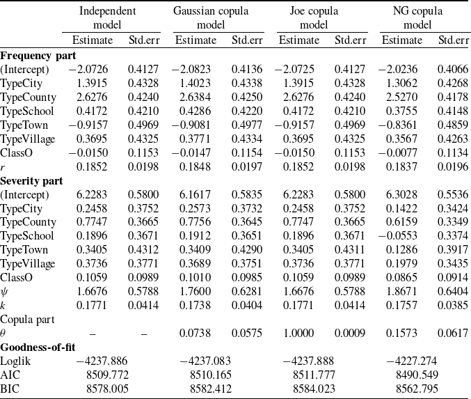
Table 6 summarizes the estimation results. The estimated copula parameters for the Gaussian and Joe models (
 $0.0738$
and
 $1.0000$
, respectively) indicate weak dependencies, suggesting they offer minimal improvement over the independent copula model. In contrast, the estimated NG copula parameter (
 $0.1573$
) implies a moderate level of the monotone decreasing conditional variance property, which the Gaussian and Joe copulas cannot adequately model. The NG copula model demonstrates the best goodness-of-fit (in terms of AIC and BIC), highlighting the importance of capturing the dataset’s monotone conditional variance characteristic.
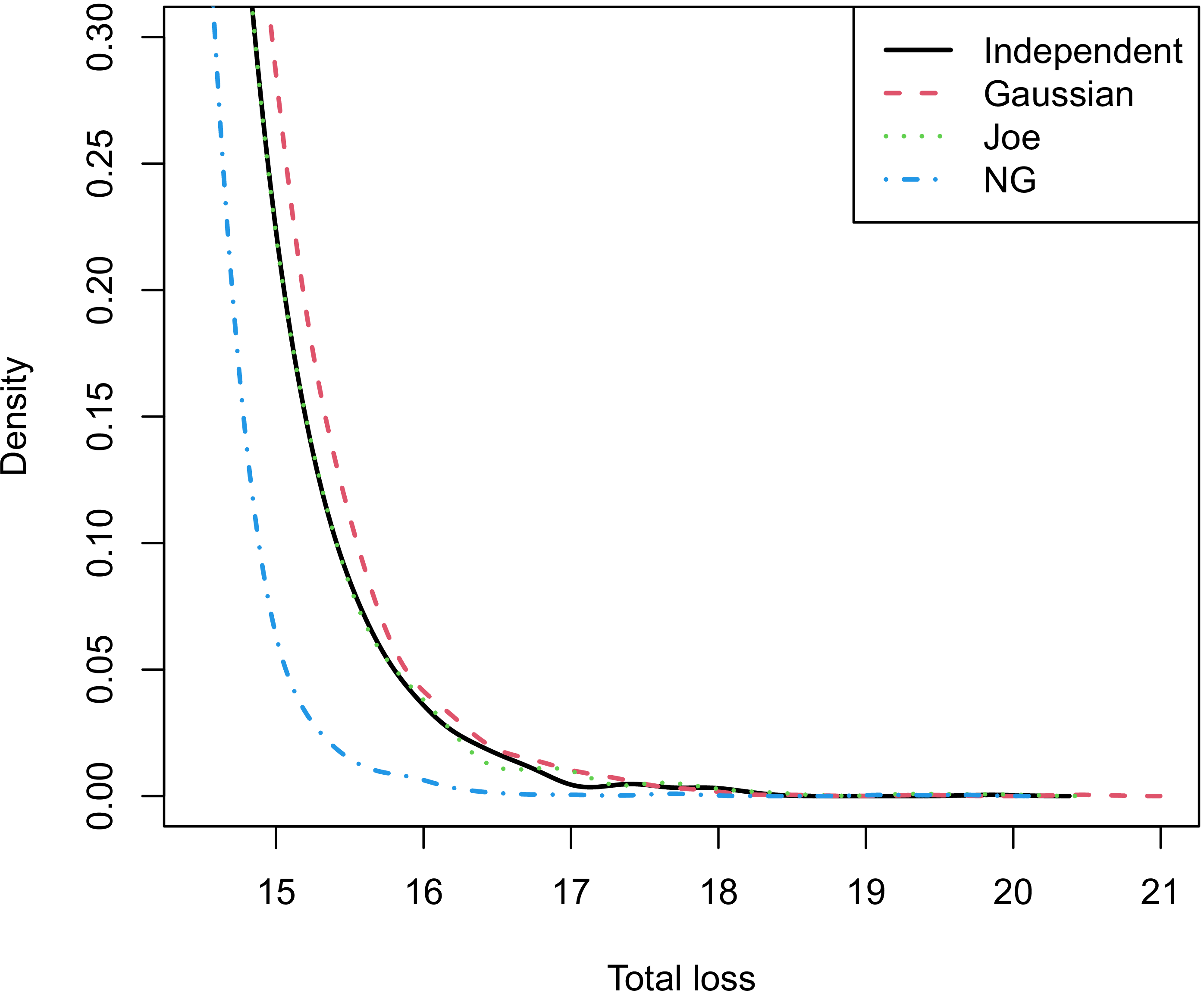
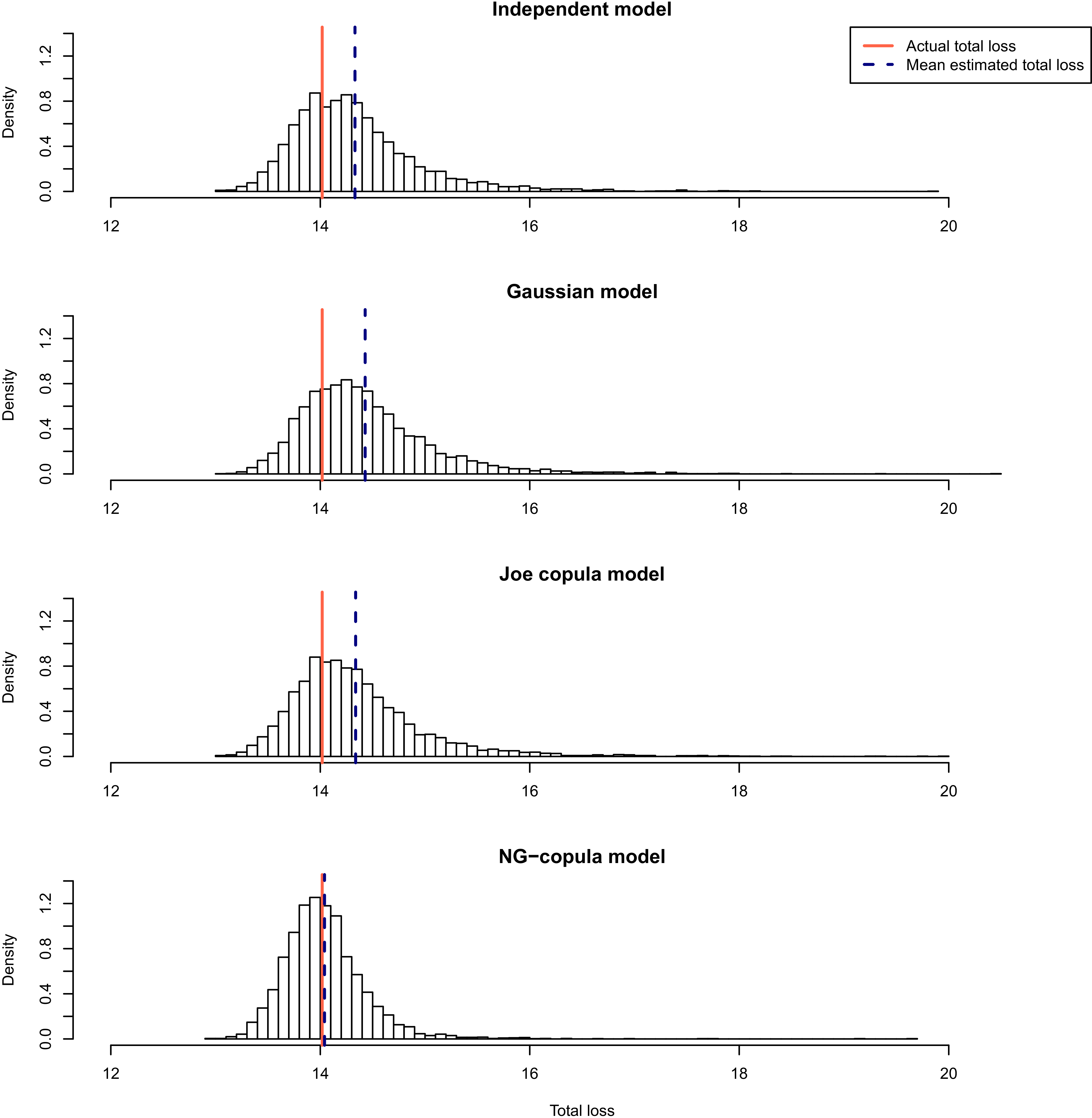
To validate these findings, we compared the four models’ total loss predictions for the 716 policyholders in the hold-out sample (year 2011). Figure 4 shows the right tails of the predictive distributions for the logarithm of total aggregated losses. The NG copula model exhibits a significantly lighter right tail, attributed to its decreasing conditional variance property. This aligns with the observations from the numerical study in Figure 3. Figure 5 shows predictive distributions for the logarithm of total aggregated losses from the four models (based on 5000 simulations using each model’s estimated parameters). The solid vertical line marks the actual hold-out sample loss (14.02), and the dashed line represents the mean estimated total loss.
Right tail of the predictive distribution for the logarithm of total aggregated losses (hold-out sample).

Predictive distribution for the logarithm of total aggregated losses (hold-out sample).

Lastly, Table 7 summarizes the predictive distributions of the total aggregated losses from the hold-out sample (minimum, quartiles, maximum, mean, and standard deviation). It is shown that the NG copula model’s predictive distribution exhibits the least variation, and its mean is closest to the actual hold-out sample loss. The Gaussian and Joe copula models, with their estimated
 $\theta$
values, essentially behave like the independent copula. They fail to capture the dataset’s dependence structure. Conversely, the NG copula model effectively models this dependence through its decreasing conditional variance property. In other words, it naturally reflects the situation where the dispersion of average severity decreases as we have more claim frequencies. This leads to its outperformance on both hold-out sample prediction and in-sample goodness-of-fit.
7. Conclusion
This paper studied copula-based dependence modeling between claim frequency and average severity in CRMs. We showed that this dependence has a nonstandard structure, especially through the stochastically monotone wing property/the monotone conditional variance property, which are not well captured by standard copula families. To address this issue, we introduced the NG copula and demonstrated, through numerical and real data analyses, that it can effectively model this type of dependence.
One limitation of the current framework is that it is mainly developed for a one-period setting. In particular, the treatment of zero frequency through an auxiliary variable is convenient here, but makes multi-year extensions less straightforward. Extending the proposed framework to longitudinal settings and developing other copula families with similar dependence properties are natural directions for future research.
Summary statistics for the total aggregated losses (log scale) from the hold-out sample.

Table 7. Long description
A table comparing summary statistics for total aggregated losses from a hold-out sample. The table has five rows and six columns. The columns are labeled Model, Min., Q1, Q2, Q3, Max., Mean, and SD. The rows are labeled Independent, Gaussian, Joe, and NG copula. Row 1: Independent, Min., 13.03, Q1, 13.93, Q2, 14.23, Q3, 14.59, Max., 19.86, Mean, 14.33, SD, 0.62. Row 2: Gaussian, Min., 13.09, Q1, 14.00, Q2, 14.32, Q3, 14.70, Max., 20.47, Mean, 14.43, SD, 0.64. Row 3: Joe, Min., 13.02, Q1, 13.93, Q2, 14.23, Q3, 14.59, Max., 19.99, Mean, 14.34, SD, 0.64. Row 4: NG copula, Min., 12.96, Q1, 13.79, Q2, 14.00, Q3, 14.22, Max., 19.63, Mean, 14.04, SD, 0.40.
Acknowledgments
The authors thank an editor and anonymous referees for their insightful comments, which significantly improved the paper.
Funding statement
Jae Youn Ahn was supported by the National Research Foundation of Korea (NRF) funded by the Ministry of Education (2021R1A6A1A10039823) and by the Ministry of Science and ICT (RS-2025-23524530). Himchan Jeong was supported by the Natural Sciences and Engineering Research Council of Canada (NSERC) Discovery Fund (RGPIN-2021-02622).
Data availability statement
The dataset used in this paper is publicly available at https://sites.google.com/a/wisc.edu/jed-frees/.
Competing interests
The authors have no potential competing or conflicting interests to declare.
Appendix A. Example of motivation
The collective risk model specified in Model 2 assumes independence between the positive frequency and the individual severities. However, this assumption seldom holds in real-world data analysis. To address this limitation, Garrido et al. (Reference Garrido, Genest and Schulz2016) proposed a generalization that models the dependence between the positive frequency and the individual severities, where the independence constraint is relaxed by allowing the conditional mean of the severity to depend on the frequency.
Specifically, for the joint modeling of the positive frequency and the positive average severity,
 $(N^+,M^+)$
, consider the setting in Model 2 with part ii replaced with
-
ii. Conditioned on
$N^+ = n \in \mathbb{N}_{\gt 0}$
, the random variables
$Z_1, Z_2, \dots, Z_n$
are independent and identically distributed (i.i.d.) following the
$\textrm{Gamma}\left(a, \frac{b}{\textrm{exp}\left(c n\right)}\right)$
distribution for some constant
$c \in \mathbb{R}$
.


Under this modification, we have
 \[M^+ \,|\, N^+ \sim \textrm{Gamma}\left(aN^+, \frac{bN^+}{\textrm{exp}\left(c N^+\right)}\right).\]
Furthermore, the conditional mean and the conditional variance are given by
 \begin{equation}{\mathbb E}\left[M^+ \,|\, N^+\right]=\frac{a}{b}\textrm{exp}\left(c N^+\right) \quad\hbox{and}\quad{\mathrm Var}\left(M^+ \,|\, N^+\right) =\frac{\left( {\mathbb E}\left[M^+ \,|\, N^+\right]\right)^2}{aN^+},\end{equation}
respectively. We emphasize that the conditional variance in (A1) decreases with
 $N^+$
if and only if the function
 $\eta: \mathbb{N}_{\gt 0} \rightarrow \mathbb{R}_{\gt 0}$
, defined as
 \[\eta(n) = \frac{\textrm{exp}\left(2c n\right)}{n}, \qquad n \in \mathbb{N}_{\gt 0},\]
is a decreasing function.
When there is a negative dependence between the frequency and the severity, equivalently
 $c \lt 0$
, then
 $\eta$
is a decreasing function. Consequently, the conditional variance in (A1) decreases as the frequency increases. In contrast, when there is a positive dependence, equivalently
 $c \gt 0$
, the conditional variance of
 $M^+$
is generally not guaranteed to decrease. However, when
 $c \gt 0$
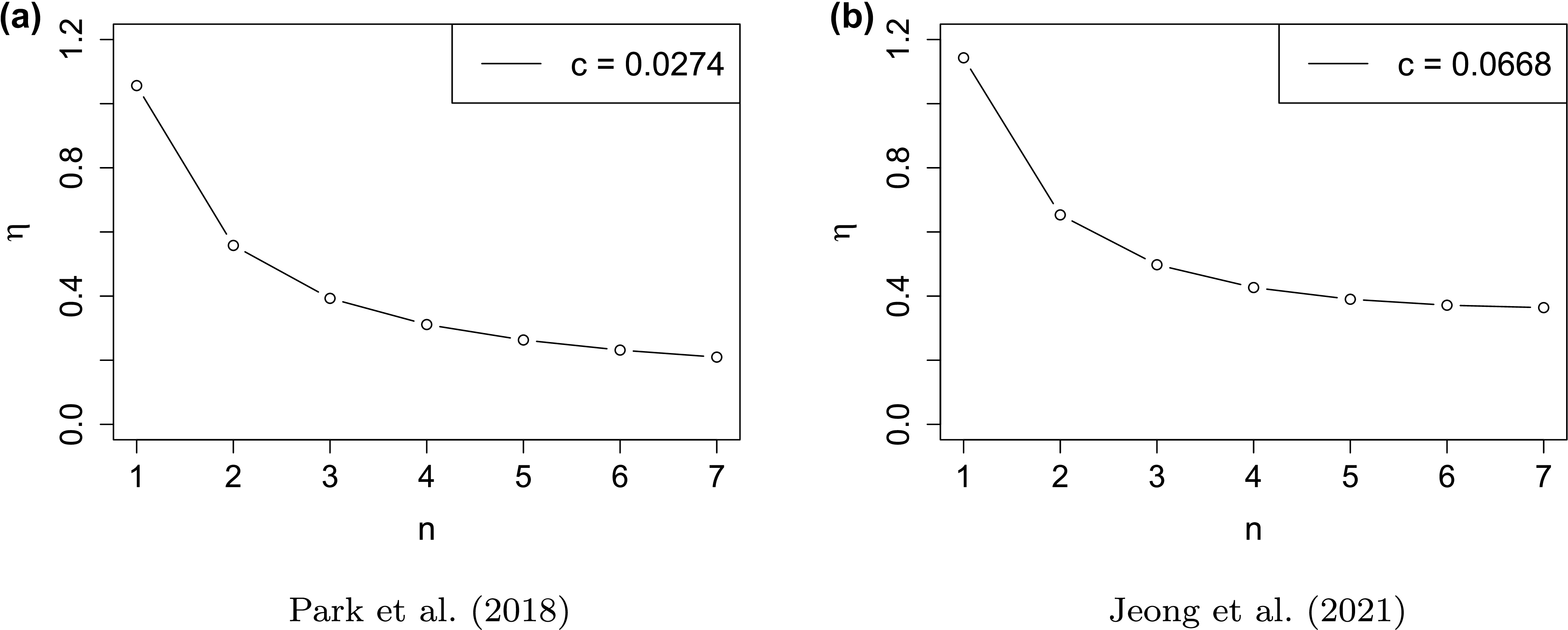
is small – a situation commonly observed in real data analysis within the insurance literature (Shi et al., Reference Shi, Feng and Ivantsova2015; Jeong et al., Reference Jeong, Valdez, Ahn and Park2021; Park et al., Reference Park, Kim and Ahn2018) – the conditional variance in (A1) is typically observed to decrease with the frequency
 $N^+ = n$
for moderate values of
 $n \in \mathbb{N}_{\gt 0}$
, as illustrated in Figure A1.
Decreasing patterns of the
 $\eta$
function for various c values.

Appendix B. Proof of Theorem 3.8
Before we give the proof of Theorem 3.8, we explore some auxiliary results.
Lemma B.1. For a fixed
 $u\in(0,1)$
, let
 \begin{equation}x^* = G^{-1}(u;\;1/\theta,1).\end{equation}
Then, as
 $\theta \to 0$
,
 \[ \lim\limits_{\theta \searrow 0}\theta \, x^* = 1. \]
Proof. Let
 $n = \tfrac{1}{\theta}$
. Define
 $W_i \stackrel{\mathrm{iid}}{\sim} G(1,1)$
, we have
 \[ X_n \;:\!=\; W_1 + W_2 + \cdots + W_n \;\sim\; G(n,1).\]
Define
 \[ F_n(z) = \mathbb{P}\bigg(\frac{X_n - n}{\sqrt{n}} \;\le\; z\bigg).\]
By the central limit theorem,
 \begin{equation} F_n(z) = \Phi(z) + o(1) \quad \text{as} \quad n \to \infty.\end{equation}
Next, from (B1) we have
 \[ u = \mathbb{P}\bigl(X_n \le x^*\bigr) = \Phi\bigg(\frac{x^* - n}{\sqrt{n}}\bigg) + o(1),\]
where the last step follows from (B2). Since
 $\Phi(\!\cdot\!)$
is strictly increasing and continuously differentiable, the mean-value theorem applied to the above asymptotic implies
 \[ \frac{x^* - n}{\sqrt{n}} = \Phi^{-1}(u) + o(1) \quad \text{as} \quad n \to \infty,\]
which completes the proof.
Lemma B.2. For a fixed
 $v\in(0,1)$
, let
 $ y^* = \Phi_{2/\theta}^{-1}(v;\;0, \theta)$
. Then
 \[ \lim\limits_{\theta \searrow 0}\frac{y^*}{\sqrt{\theta}} = \Phi^{-1}(v). \]
Proof. Define
 \[ \widetilde{\Phi}_{\theta}(z) = \Phi_{2/\theta}\bigl(z\sqrt{\theta};\; 0, \theta \bigr), \quad z\in\mathbb{R}.\]
Note that the t-distribution is a location-scale family, and hence we have
 \[ \widetilde{\Phi}_\theta(z) = \Phi_{2/\theta}(z\sqrt{\theta};\; 0, \theta) = \Phi_{2/\theta}(z;\; 0,1).\]
Since
 $y^* = \Phi_{2/\theta}^{-1}(v;\;0,\theta)$
, setting
 $ z^* ={y^*}/{\sqrt{\theta}} $
implies that
 \[\widetilde{\Phi}_{\theta}(z^*) = \Phi_{2/\theta}(y^*;\;0,\theta)= v.\]
Next, by the convergence of the t-distribution to the normal distribution as the degrees of freedom tend to infinity, we have
 \[ \sup_{z\in\mathbb{R}} \bigl|\widetilde{\Phi}_{\theta}(z) - \Phi(z)\bigr| = \sup_{z\in\mathbb{R}} \bigl|\Phi_{2/\theta}(z;\;0,1) - \Phi(z)\bigr| \;\longrightarrow\; 0 \quad\text{as}\quad \theta\searrow 0.\]
Hence, for our specific
 $z^*$
,
 $ v = \widetilde{\Phi}_{\theta}(z^*) = \Phi(z^*) + o(1).$
Since
 $\Phi(\!\cdot\!)$
is strictly increasing and continuous, applying its inverse function to both sides yields
 \[ z^* = \Phi^{-1}(\Phi(z^*)) = \Phi^{-1}(v - o(1)).\]
A Taylor expansion of
 $\Phi^{-1}$
around v then implies that
 $z^* = \Phi^{-1}(v) + o(1)$
. Consequently,
 \[ y^* = \sqrt{\theta}\,z^* = \sqrt{\theta}\,\Phi^{-1}(v) + o(\sqrt{\theta}),\]
which completes the proof.
Lemma B.3. For fixed
 $v \in (0,1)$
,
 \begin{equation} \lim\limits_{\theta\searrow 0}\left[\phi_{2/\theta}(y^*;\;0,\theta)-\frac{1}{\sqrt{2\pi\theta}}\, \exp\!\bigg(-\frac12\,\bigl[\Phi^{-1}(v)\bigr]^2\bigg)\right] =0 \end{equation}
and
 \begin{equation} \lim\limits_{\theta\searrow 0}\frac{1}{\theta}\left[\frac{1}{\phi_{2/\theta}(y^*;\;0,\theta)}-\sqrt{2\pi\theta}\,\exp\!\bigg(\frac12\,\bigl[\Phi^{-1}(v)\bigr]^2\bigg)\right]=0\end{equation}
as
 $\theta \searrow 0$
, where
 $y^* = \Phi_{2/\theta}^{-1}(v;\;0,\theta)$
.
Proof. The following is well-known
 \begin{equation} \phi_{n}(z;\; 0,1) = \frac{1}{\sqrt{2\pi}}\, \exp\!\bigg(-\frac{z^2}{2}\bigg) + o(1) \quad \text{as } n \rightarrow \infty\end{equation}
for
 $z \in \mathbb{R}$
; see, for example Johnson et al. (Reference Johnson, Kotz and Balakrishnan1995). Next, recall from Lemma 9.2 that for fixed
 $v\in (0,1)$
,
 \begin{equation} y^* = \sqrt{\theta}\,\Phi^{-1}(v) + o(\sqrt{\theta}), \quad \text{as } \theta \searrow 0,\end{equation}
where
 $y^* = \Phi_{2/\theta}^{-1}(v;\;0,\theta)$
. Define
 $ z^* = {y^*}/{\sqrt{\theta}}$
, so that (B6) implies
 $z^* = \Phi^{-1}(v) + o(1)$
as
 $ \theta \searrow 0$
. We apply (B5) to get
 \[ \phi_{2/\theta}(z^*;\; 0,1) = \frac{1}{\sqrt{2\pi}}\, \exp\bigg(-\frac{\bigl(\Phi^{-1}(v) + o(1)\bigr)^2}{2}\bigg) \quad \text{as } \theta \searrow 0.\]
By the standard location-scale relation for the t-density,
 \[ \phi_{2/\theta}(y^*;\;0,\theta) = \frac{1}{\sqrt{\theta}} \,\phi_{2/\theta}\!\bigg(\frac{y^*}{\sqrt{\theta}};\; 0, 1\bigg).\]
Hence,
 \[\begin{aligned} \phi_{2/\theta}(y^*;\;0,\theta) & = \frac{1}{\sqrt{\theta}}\,\ \phi_{2/\theta}(z^*;\; 0,1) \\ &= \frac{1}{\sqrt{\theta}}\, \frac{1}{\sqrt{2\pi}}\, \exp\bigg(-\frac{[\Phi^{-1}(v)+o(1)]^2}{2}\bigg) \\ &= \frac{1}{\sqrt{2\pi\,\theta}}\, \exp\bigg(-\frac{[\Phi^{-1}(v)]^2}{2}\bigg) + o(1),\end{aligned}\]
where the final equality uses a Taylor expansion in the o(1) term. This proves (B3).
We now prove (B4). From (B3) we see that
 \begin{equation}\phi_{2/\theta}(y^*;\;0,\theta) = \frac{A}{\sqrt{\theta}} + o(1),\end{equation}
where
 \[ A \;:\!=\; \frac{1}{\sqrt{2\pi}} \,\exp\bigg(-\frac12\,\bigl[\Phi^{-1}(v)\bigr]^2\bigg).\]
Inverting (B7) and using the Taylor expansion, we obtain
 \[\begin{aligned}\frac{1}{\phi_{2/\theta}(y^*;\;0,\theta)} &= \frac{\sqrt{\theta}}{A + o(\sqrt{\theta})}= \frac{\sqrt{\theta}}{A} + o(\theta).\end{aligned}\]
Since
 $\frac{1}{A} = \sqrt{2\pi}\,\exp\!\bigl(\tfrac12\,(\Phi^{-1}(v))^2\bigr)$
, we have
 \[\frac{1}{\phi_{2/\theta}(y^*;\;0,\theta)} = \sqrt{2\pi\,\theta}\,\exp\bigg(\frac12\,\bigl[\Phi^{-1}(v)\bigr]^2\bigg) + o\bigl(\theta\bigr),\]
which establishes (B4) and completes the proof.
Proof of Theorem 3.8. First, note that the copula density function is given by
 \[ c_{\theta}(u,v) = \frac{1}{\sqrt{2\pi}} \left(x^*\right)^{1/2} \exp\bigg(-\frac12\,x^*\,(y^*)^2\bigg) \frac{1}{\phi_{2/\theta}(y^*;\;0,\theta)},\]
where
 $x^* = G^{-1}(u;\;1/\theta,1)$
and
 $ y^* = \Phi_{2/\theta}^{-1}(v;\;0,\theta)$
.
Lemma B.1 implies
 \begin{equation} \left(x^*\right)^{1/2} = \Bigl(\tfrac{1}{\theta} + o\bigl(\tfrac{1}{\theta}\bigr)\Bigr)^{1/2} = \frac{1}{\sqrt{\theta}} \,\bigl[1 + o(1)\bigr]\quad \hbox{as} \quad \theta\searrow 0.\end{equation}
From Lemma B.2,
 \[ y^* = \sqrt{\theta}\,\Phi^{-1}(v) + o\bigl(\sqrt{\theta}\bigr) \quad \hbox{as} \quad \theta\searrow 0,\]
we also have
 \[ (y^*)^2 = \theta\,\bigl[\Phi^{-1}(v)\bigr]^2 + o(\theta) \quad\Longrightarrow\quad x^*\,(y^*)^2 = \bigl[\Phi^{-1}(v)\bigr]^2 + o(1)\]
as
 $\theta\searrow 0$
. Therefore, using a Taylor expansion and Lemma 9.1, we have
 \begin{equation} \exp\bigg(-\frac12\,x^*\,(y^*)^2\bigg) = \exp\bigg(-\frac12\,\bigl[\Phi^{-1}(v)\bigr]^2\bigg) \,\bigl[\,1 + o(1)\bigr] \quad \hbox{as} \quad \theta\searrow 0.\end{equation}
Finally, using (B8), (B9), and Lemma B.3, we get
 \[\begin{aligned} c_{\theta}(u,v) &= \frac{1}{\sqrt{2\pi}} \left(x^*\right)^{1/2} \exp\bigg(-\frac12\,x^*\,(y^*)^2\bigg) \frac{1}{\phi_{2/\theta}(y^*;\;0,\theta)} \\ &= \frac{1}{\sqrt{2\pi}} \Bigl(\frac{1}{\sqrt{\theta}}[1+o(1)]\Bigr) \Bigl(\exp\!\bigg(-\frac12[\Phi^{-1}(v)]^2\bigg)[1+o(1)]\Bigr) \Bigl(\sqrt{2\pi\,\theta}\exp\!\bigg(\frac12[\Phi^{-1}(v)]^2\bigg)+o(\theta)\Bigr) \\ &= (1+o(1))\, \exp\!\bigg(-\frac12[\Phi^{-1}(v)]^2\bigg)\, \left(\left(\exp\!\bigg(\frac12[\Phi^{-1}(v)]^2\bigg)\right) + o(\sqrt{\theta})\right) \\ &= 1 + o(1)\end{aligned}\]
as
 $\theta\searrow 0$
.
Appendix C. Proof of Theorem 3.9
First, define the constant
 \[s_0 = \int_{0}^{e^{-\gamma}} \eta_1(s)\log s \, ds + \int_{e^{-\gamma}}^{\infty} \eta_2(s)\log s \, ds,\]
where
 $\eta_1(s)=(e^{-s}-1)/s$
,
 $\eta_2(s)={e^{-s}}/{s}, $
and
 $\gamma$
denotes the Euler–Mascheroni constant defined as
 \[\gamma = \lim_{n \to \infty} \left( \sum_{k=1}^{n} \frac{1}{k} - \ln n \right),\]
which satisfies
 $\gamma\gt 0$
. Numerical evaluation gives
 $0\lt s_0$
≃
 $0.4617819158$
(Pedersen, Reference Pedersen2026). The following lemma describes the asymptotic behavior of the quantiles of the gamma distribution as the shape parameter approaches zero with the rate parameter fixed at 1.
Lemma C.1 For
 $u\in(0,1)$
and
 $\theta\gt 0$
, let
 $q_\theta(u)$
denote the u-th quantile of the
 $\mathrm{Gamma}(1/\theta,1)$
distribution. Then,
-
i. As
$\theta\to\infty$
, where
\[ q_\theta(u) = u^{\theta}(c+O(1/\theta)), \]
$c=e^{-\gamma} s_0 \gt 0$
.
-
ii. For any
$u_1, u_2\in(0,1)$
with
$u_1\gt u_2$
,
\[ \lim_{\theta\to\infty} \frac{q_\theta(u_2)}{q_\theta(u_1)}=0. \]
-
iii. Let
$U_1, U_2 \sim \operatorname{Unif}(0,1)$
and
$Z_1, Z_2 \sim N(0,1)$
be mutually independent, and define Then,
\[ Y_i = \frac{|Z_i|}{q_\theta(U_i)}, \quad i=1,2. \]
\[ \lim_{\theta\to\infty} \mathbb{P}((Y_2 - Y_1)(q_\theta(U_2) - q_\theta(U_1)) \lt 0) = 1.\]


Proof. Part i follows from the main expansion in Pedersen (Reference Pedersen2026). The proof of part ii immediately follows from part i.
For the proof of part iii, since
 ${\mathbb{P}}\left(\left\vert Z_1 \right\vert\gt 0,\, U_1\gt 0\right)=1$
for given
 $\theta\gt 0$
, it is enough to prove
 \begin{equation} \lim\limits_{\theta\rightarrow \infty} {\mathbb{P}}\left(\left.\left( Y_2-Y_1\right)\left(q_\theta\left(U_2\right)-q_\theta\left(U_1\right)\right)\lt 0 \,\right\vert\, \left\vert Z_1 \right\vert\gt 0, U_1\gt 0\right)=1. \end{equation}
By the symmetricity, for the proof of (C1), it is enough to show
 \[ \begin{aligned} &\lim\limits_{\theta\rightarrow \infty} {\mathbb{P}}\left(\left.Y_2\gt Y_1 \,\right\vert\, U_2\lt U_1, \left\vert Z_1 \right\vert\gt 0, U_1\gt 0\right)\\ &\quad\quad= \lim\limits_{\theta\rightarrow \infty}{\mathbb{P}}\left(\left.\frac{\left\vert Z_2\right\vert}{\left\vert Z_1 \right\vert} \gt \frac{q_\theta\left(U_2\right)}{q_\theta\left(U_1\right)}\,\right\vert\, U_2\lt U_1, \left\vert Z_1 \right\vert\gt 0, U_1\gt 0\right)\\ &\quad\quad={\mathbb{P}}\left(\left.\frac{\left\vert Z_2\right\vert}{\left\vert Z_1\right\vert} \gt 0\,\right\vert\, U_2\lt U_1, \left\vert Z_1 \right\vert\gt 0, U_1\gt 0\right)\\ &\quad\quad={\mathbb{P}}\left(\left.\frac{\left\vert Z_2\right\vert}{\left\vert Z_1\right\vert} \gt 0\,\right\vert\, \left\vert Z_1 \right\vert\gt 0\right)\\ &\quad\quad=1, \end{aligned} \]
where the first equality is from the monotonicity of the quantile function, and the second equality comes from the dominant convergence theorem as well as the result in part ii, and the third equality is from the independence assumption.
Proof of Theorem 3.9. We provide the proof of part i; the proof of part ii follows similarly.
Showing part i is equivalent to show that as
 $\theta\to\infty$
the NG copula exhibits asymptotically countermonotonic behavior in the upper tail (i.e. when
 $V\gt 1/2$
). By invariance of the copula under strictly increasing transformations, it suffices to work with the representation of the NG distribution. Using the representation in Model 3, we represent the random vector from the NG distribution
 $H_{1/\theta,1}$
, via the quantile transformation. Let
 \[X_i = q_{\theta}(U_i),\quad Y_i = \frac{Z_i}{\,q_{\theta}(U_i)},\quad i=1,2,\]
where
 $q_\theta(u)$
denotes the u-th quantile of the
 $\operatorname{Gamma}(1/\theta,1)$
distribution,
 $U_i\sim \operatorname{Unif}(0,1)$
, and
 $Z_i\sim N(0,1)$
are mutually independent. We also define
 \[ Y_i^* = \frac{\left\vert Z_i\right\vert}{\,q_{\theta}(U_i)\!}. \]
Then, we have that
 $(X_1, X_2)$
and
 $(Y_1, Y_2)$
are independent copies drawn from
 $H_{1/\theta,1}$
.
By the symmetry of the Student’s t-distribution, the countermonotonic behavior of the NG copula in the upper tail
 $V\gt 1/2$
is equivalent to the countermonotonic behavior of the NG distribution in the upper tail
 $Y\gt0$
. Thus, it suffices to show
 \[\lim_{\theta\to\infty}{\mathbb{P}}((Y_2-Y_1)(X_2-X_1)\lt 0 \,|\, Y_1\gt 0,\,Y_2\gt 0)=1.\]
This can be obtained from
 \[ \begin{aligned} \lim_{\theta\to\infty}{\mathbb{P}}\left(\left.(Y_2-Y_1)(X_2-X_1)\lt 0 \,\right\vert Y_1\gt 0, Y_2\gt 0\right) &={\mathbb{P}}\left((Y_2^*-Y_1^*)(X_2-X_1)\lt 0 \right)\\ &=1, \end{aligned}\]
where the first equality is from the symmetric property of the standard normal distribution, and the second equation is from part iii of Lemma C.1.


 (N+,M+)
 θ=(0.1,0.5,1,5,10,30)
 %
 N+
 M+

 η


