1 Introduction
The nonlinear evolution of Langmuir waves has been studied in great detail in part because these waves are often found in nature (LaBelle, Cairns & Kletzing Reference LaBelle, Cairns and Kletzing2010; Briand Reference Briand2015) and are easily excited in a laboratory, but also because they can serve as a reference case for illustrating some general nonlinear wave phenomena. Many, or most, of the early analytical studies (Nishikawa Reference Nishikawa1968; Ichikawa, Imamura & Taniuti Reference Ichikawa, Imamura and Taniuti1972; Weiland & Wilhelmsson Reference Weiland and Wilhelmsson1977) addressed single-wave modes modulated by some means. In nature, in particular, such plane wave modes are found only very rarely, and studies of broad spectra are more relevant. Unfortunately, the results from single-mode studies are not readily generalized to a turbulent spectrum. This latter case will be analysed in the present work, beginning with the simplest non-trivial extension where two-wave modes are present initially with their internal phase relations suppressed.
A basic and widely applied mathematical model for the nonlinear Langmuir wave problem in isotropic homogeneous thermal plasmas (Zakharov Reference Zakharov1972; Kono & Škorić Reference Kono and Škorić2010) was found by removing the rapidly varying, high-frequency part of the wave field by the standard substitution
 $\boldsymbol{E}\rightarrow \boldsymbol{E}(\boldsymbol{r},t)\exp (-\text{i}\unicode[STIX]{x1D714}_{o}t)$
, with
 $\unicode[STIX]{x1D714}_{0}$
being the carrier wave frequency, here taken to be the plasma frequency
 $\unicode[STIX]{x1D714}_{pe}$
. When
 $\unicode[STIX]{x2202}\boldsymbol{E}/\unicode[STIX]{x2202}t\ll \unicode[STIX]{x1D714}_{0}\boldsymbol{E}$
we have
 $$\begin{eqnarray}\left(i\frac{\unicode[STIX]{x2202}}{\unicode[STIX]{x2202}t}+\frac{1}{2}\frac{\unicode[STIX]{x1D710}^{2}}{\unicode[STIX]{x1D714}_{pe}}\unicode[STIX]{x1D6FB}^{2}\right)\boldsymbol{E}=\frac{1}{2}\unicode[STIX]{x1D714}_{pe}\left(\frac{\widetilde{n}}{n_{0}}\boldsymbol{E}\right),\end{eqnarray}$$
with
 $\widetilde{n}$
being the slowly varying perturbation of the reference density
 $n_{0}$
, and
 $\unicode[STIX]{x1D710}\equiv \sqrt{3T_{e}/m}$
. Implicit in (1.1) lies an assumption of electrostatic waves with
 $\boldsymbol{E}=-\unicode[STIX]{x1D735}\unicode[STIX]{x1D719}$
, i.e.
 $\unicode[STIX]{x1D735}\times \boldsymbol{E}\approx 0$
. Self-consistency requires that the right-hand side of (1.1) has no sources for a rotation of the electric field, implying
 $\boldsymbol{E}\times \unicode[STIX]{x1D735}(\widetilde{n}/n_{0})\approx 0$
.
The expression (1.1) applies for prescribed variations of the bulk quasi-neutral plasma density
 $\widetilde{n}$
but is most interesting for a self-consistent dynamic problem where the density perturbations are nonlinearly coupled to the electric field by
 $$\begin{eqnarray}\left(\frac{\unicode[STIX]{x2202}^{2}}{\unicode[STIX]{x2202}t^{2}}-C_{s}^{2}\unicode[STIX]{x1D6FB}^{2}\right)\frac{\widetilde{n}}{n_{0}}=\frac{\unicode[STIX]{x1D700}_{0}}{2Mn_{0}}\unicode[STIX]{x1D6FB}^{2}|E|^{2},\end{eqnarray}$$
to be completed with initial conditions. The ion component was assumed to be cold, giving the sound speed
 $C_{s}\equiv \sqrt{T_{e}/M}$
in terms of the electron temperature
 $T_{e}$
and ion mass
 $M$
. Finite ion temperatures in a fluid model give no difference of substance, but ion kinetic effects will give important modifications (Dysthe & Pécseli Reference Dysthe and Pécseli1977; Shatashvili & Tsintsadze Reference Shatashvili and Tsintsadze1982). Equations (1.1) and (1.2) constitute the so called Zakharov equations (Zakharov Reference Zakharov1972) in a simplified form. The basic set of (1.1) and (1.2), as they stand, can describe decay of Langmuir waves, modulational instabilities as well as Langmuir wave collapse in three-dimensional plasmas (Zakharov Reference Zakharov1972; Rasmussen & Rypdal Reference Rasmussen and Rypdal1986).
Relations (1.1) and (1.2) correspond to the linear Langmuir wave dispersion relation in the limiting form
 $$\begin{eqnarray}\unicode[STIX]{x1D714}=\unicode[STIX]{x1D714}_{pe}\left(1+{\textstyle \frac{3}{2}}(k\unicode[STIX]{x1D706}_{De})^{2}\right),\end{eqnarray}$$
with a standard notation where
 $\unicode[STIX]{x1D706}_{De}$
is the Debye length. The fast variation on the time scale
 $\unicode[STIX]{x1D714}_{pe}^{-1}$
is subsequently removed.
A critical wavenumber
 $k_{c}$
can be defined from (1.3) by equalling the group velocity
 $u_{g}$
of the Langmuir waves with the ion sound speed. Langmuir waves with wavenumber
 $k>k_{c}$
can decay to another Langmuir wave and an ion sound wave (Tanaka Reference Tanaka1977a
,Reference Tanaka
b
). For
 $k<k_{c}$
only the modulational instability remains (Thornhill & ter Haar Reference Thornhill and ter Haar1978). With the Langmuir wave dispersion relation (1.3) we find
 $$\begin{eqnarray}k_{c}=\frac{1}{3}\frac{C_{s}}{\unicode[STIX]{x1D714}_{pe}\unicode[STIX]{x1D706}_{De}^{2}}=\frac{1}{3}\frac{1}{\unicode[STIX]{x1D714}_{pe}\unicode[STIX]{x1D706}_{De}^{2}}\sqrt{\frac{T_{e}}{M}}=\frac{1}{3}\sqrt{\frac{m}{M}}\frac{1}{\unicode[STIX]{x1D706}_{De}}.\end{eqnarray}$$
Based on the set of (1.1) and (1.2), previous studies (Pécseli Reference Pécseli2014) found the, in general, complex dispersion relation
 $$\begin{eqnarray}\displaystyle W^{2}-C_{s}^{2}K^{2}=-\frac{\unicode[STIX]{x1D700}_{0}\unicode[STIX]{x1D714}_{pe}}{8Mn_{0}}K^{2}\,\iiint _{-\infty }^{\infty }\frac{G_{0}\left(\boldsymbol{k}+\displaystyle \frac{1}{2}\boldsymbol{K}\right)-G_{0}\left(\boldsymbol{k}-\displaystyle \frac{1}{2}\boldsymbol{K}\right)}{W-\displaystyle \frac{\unicode[STIX]{x1D710}^{2}}{\unicode[STIX]{x1D714}_{pe}}\boldsymbol{k}\boldsymbol{\cdot }\boldsymbol{K}}\,\text{d}k^{3}, & & \displaystyle\end{eqnarray}$$
which reduces to
 $$\begin{eqnarray}\displaystyle W^{2}-C_{s}^{2}K^{2}=\frac{\unicode[STIX]{x1D700}_{0}\unicode[STIX]{x1D710}^{2}}{8Mn_{0}}K^{4}\,\iiint _{-\infty }^{\infty }\frac{G_{0}(\boldsymbol{k}^{\prime })}{\left(W-\displaystyle \frac{\unicode[STIX]{x1D710}^{2}}{\unicode[STIX]{x1D714}_{pe}}\boldsymbol{k}^{\prime }\boldsymbol{\cdot }\boldsymbol{K}\right)^{2}-\left(\displaystyle \frac{1}{2}\displaystyle \frac{\unicode[STIX]{x1D710}^{2}}{\unicode[STIX]{x1D714}_{pe}}K^{2}\right)^{2}}\,\text{d}k^{\prime \,3}, & & \displaystyle\end{eqnarray}$$
where
 $G_{0}(\boldsymbol{k})$
is the reference unperturbed wavenumber spectrum of the Langmuir waves, and a generally complex frequency,
 $W$
, accounts for the low-frequency variation and
 $\boldsymbol{K}$
is the perturbation wave vector. It will be assumed that
 $G_{0}(\boldsymbol{k})$
is centred around some carrier wavenumber
 $\boldsymbol{k}_{0}$
or possibly more than one, where a limiting case will be
 $G_{0}(\boldsymbol{k})=A^{2}\unicode[STIX]{x1D6FF}(\boldsymbol{k}-\boldsymbol{k}_{0})$
or possibly a sum of such
 $\unicode[STIX]{x1D6FF}$
functions. The analysis giving (1.5) and (1.6) introduced average
 $\boldsymbol{R}\equiv 1/2(\boldsymbol{r}_{1}+\boldsymbol{r}_{2})$
and separation
 $\boldsymbol{r}\equiv \boldsymbol{r}_{1}-\boldsymbol{r}_{2}$
coordinates, as well as average and separation times
 $T\equiv 1/2(t_{1}+t_{2})$
,
 $\unicode[STIX]{x1D70F}\equiv t_{1}-t_{2}$
, respectively (Vedenov, Gordeev & Rudakov Reference Vedenov, Gordeev and Rudakov1967; Alber Reference Alber1978). Local power spectra that depend on
 $\boldsymbol{R}$
and
 $T$
are found by Fourier transforming the general space–time varying correlation function with respect to
 $\boldsymbol{r}$
and
 $\unicode[STIX]{x1D70F}$
. The expressions (1.5) and (1.6) were derived by Pécseli (Reference Pécseli2014) using a detailed nonlinear analysis that had a wider scope than a linear dispersion relation. We found it worthwhile to illustrate also, for completeness, how the present result can be found by a somewhat simpler analysis. This is shown in appendix A.
The derivation of (1.6) was based on ideas originally formulated for studying wave mechanics (Wigner Reference Wigner1932; Leaf Reference Leaf1968), but they were later applied also to two-dimensional wavetrains on water surfaces (Alber Reference Alber1978) and electron plasma waves (Bhakta & Majumder Reference Bhakta and Majumder1983; Pécseli Reference Pécseli2014). Other models for the modulational instability of Langmuir wave spectra have been proposed as well (Breizman & Malkin Reference Breizman and Malkin1980; Malkin Reference Malkin1982). We are here only interested in unstable solutions with complex
 $W$
, so there are no problems here with singularities on the integration paths of (1.5) and (1.6) taken in the Landau sense. For a given
 $G_{0}(\boldsymbol{k})$
, expression (1.6) is unaffected by the replacement
 $(W,K)\rightarrow (-W,-K)$
, where generally
 $W=\text{Re}\{W\}+i\,\text{Im}\{W\}$
. Figures can be made compact by use of this symmetry, but a three-dimensional presentation happens to give a better overview by allowing for some redundancy. Parts of the analysis in § 2 demonstrates that (1.5) and (1.6) contain known results for weakly nonlinear single plane waves, in particular Langmuir wave decay.
The previous analysis (Pécseli Reference Pécseli2014) demonstrated how a finite bandwidth could stabilize the modulational instability of Langmuir waves. It should be pointed out here that a simple ‘wave independence’ hypothesis can be formulated where this observation could be trivial. The hypothesis states that each component of the spectrum evolves nonlinearly but independently of the others. The instabilities are nonlinear phenomena, and depend on the wave amplitude with a growth rate proportional to the wave amplitude, although not necessarily linearly proportional (Thornhill & ter Haar Reference Thornhill and ter Haar1978). The local wave amplitude in
 $\boldsymbol{k}$
-space is everywhere reduced by a spectral broadening and the instability growth rates will be reduced merely by this effect. Starting with a plane wave, we have its peak amplitude reduced by the spectral broadening, while on the other hand, waves with originally vanishing amplitude will be excited.
For the modulational instability it was easy to see that this wave independence hypothesis is in error: distributing the available energy density from one original wave mode to merely two counter-propagating waves, it was found that the entire variation of the original one mode dispersion diagram
 $W(\boldsymbol{K})$
was changed and could not be described by a superposition of the two dispersion diagrams corresponding to the two new modes. This observation refers however to modulational instabilities and it is worthwhile to test the hypothesis for the Langmuir decay instability as well. Unfortunately, the problem has many parameters and requires a large number of illustrations for summarizing even a moderate selection of the basic results.
2 Single-wave mode
A Langmuir wave spectrum composed by a sum of
 $N$
single modes, where each can be approximated by a
 $\unicode[STIX]{x1D6FF}$
function with wave amplitude
 $A_{j}$
in (1.6), is readily solved. With
 $G_{0}(\boldsymbol{k})=\sum _{j}^{N}A_{j}^{2}\unicode[STIX]{x1D6FF}(\boldsymbol{k}-\boldsymbol{k}_{0j})$
we find
 $$\begin{eqnarray}(W^{2}-C_{s}^{2}K^{2})=\frac{\unicode[STIX]{x1D700}_{0}\unicode[STIX]{x1D710}^{2}}{8Mn_{0}}K^{4}\mathop{\sum }_{j}^{N}\frac{A_{j}^{2}}{\left(W-\displaystyle \frac{\unicode[STIX]{x1D710}^{2}}{\unicode[STIX]{x1D714}_{pe}}\boldsymbol{k}_{0j}\boldsymbol{\cdot }\boldsymbol{K}\right)^{2}-\left(\displaystyle \frac{1}{2}\frac{\unicode[STIX]{x1D710}^{2}}{\unicode[STIX]{x1D714}_{pe}}K^{2}\right)^{2}}.\end{eqnarray}$$
First we consider such a single-wave mode,
 $N=1$
in (2.1), with amplitude
 $A_{0}$
and specified by its wave vector
 $\boldsymbol{k}_{0}$
. The corresponding frequency
 $\unicode[STIX]{x1D714}_{0}$
is then given through the Langmuir wave dispersion relation. Results for this particular limiting case can be obtained also from first principles by assuming a plane weakly nonlinear Langmuir wave from the outset. A standard analysis (Thornhill & ter Haar Reference Thornhill and ter Haar1978; Pécseli Reference Pécseli2014) thus gives the dispersion relation
 $$\begin{eqnarray}\frac{1}{K^{4}}(W^{2}-C_{s}^{2}K^{2})\left(\left(W-\frac{\unicode[STIX]{x1D710}^{2}}{\unicode[STIX]{x1D714}_{pe}}\boldsymbol{k}_{0}\boldsymbol{\cdot }\boldsymbol{K}\right)^{2}-\frac{\unicode[STIX]{x1D710}^{4}}{4\unicode[STIX]{x1D714}_{pe}^{2}}K^{4}\right)=\frac{\unicode[STIX]{x1D700}_{0}\unicode[STIX]{x1D710}^{2}}{8Mn_{0}}A_{0}^{2}.\end{eqnarray}$$
In (2.2) we have two natural modes of wave propagation with dispersion relations
 $W=\pm C_{s}K$
(i.e. ion-acoustic sound waves) and
 $W=(\unicode[STIX]{x1D710}^{2}/\unicode[STIX]{x1D714}_{pe})(\boldsymbol{k}_{0}\boldsymbol{\cdot }\boldsymbol{K}\pm (1/2)K^{2})$
, corresponding to propagating and dispersing Langmuir wave packets. Recall that to the present approximation we have
 $(\unicode[STIX]{x1D710}^{2}/\unicode[STIX]{x1D714}_{pe})\boldsymbol{k}_{0}$
as the Langmuir wave group velocity. The two-wave forms listed are coupled by the finite amplitude, nonlinear effects accounted for by the right-hand side of (2.2).
For presenting normalized figures we introduce the normalizations:
-
(i) frequency
 $W^{\prime }\equiv 3/2(W/\unicode[STIX]{x1D6FA}_{pi})\sqrt{M/m}$
,
-
(ii) wavenumbers
$\boldsymbol{K}^{\prime }\equiv (3/2)\boldsymbol{K}\unicode[STIX]{x1D706}_{De}\sqrt{M/m}$
and also
$\boldsymbol{k}_{0}^{\prime }\equiv (3/2)\boldsymbol{k}_{0}\unicode[STIX]{x1D706}_{De}\sqrt{M/m}$
, -
(iii) the right-hand side coupling coefficient of (2.2)
$C^{\prime }\equiv (1/2)(\unicode[STIX]{x1D700}_{0}A_{0}^{2}/n_{0}T_{e})3/4(M/m)$
,




where
 $^{\prime }$
will denote normalized quantities throughout, and not differentiations.
Decaying Langmuir wavenumbers will be found for
 $|k_{0}|\geqslant k_{c}\equiv 1/3\sqrt{m/M}/\unicode[STIX]{x1D706}_{De}$
as also demonstrated by a simple geometrical construction using the linear dispersion relation (Thornhill & ter Haar Reference Thornhill and ter Haar1978). To be consistent with the ordering in (1.1) and (1.2), where
 $\sqrt{m/M}$
is a small parameter, we require low-frequency modulations to have frequencies
 $W\leqslant \unicode[STIX]{x1D6FA}_{pi}\sqrt{m/M}$
and wavenumbers
 $|K|\leqslant \sqrt{m/M}/\unicode[STIX]{x1D706}_{De}$
, giving
 $|k_{0}^{\prime }|\leqslant 1$
,
 $W^{\prime }\leqslant 1$
and
 $|K^{\prime }|\leqslant 1$
, although some of these constraints can be relaxed slightly. We also have
 $|W^{\prime }/K^{\prime }|=|W/K|/\unicode[STIX]{x1D706}_{De}\unicode[STIX]{x1D6FA}_{pi}=|W/K|/C_{s}$
. Taking a wave with energy density
 $(1/2)\unicode[STIX]{x1D700}_{0}E^{2}\approx (m/M)n_{0}T_{e}$
will imply
 $C^{\prime }\approx 3/4$
. These normalized units will be used for numerical solutions of dispersion relations. In these units we find the ion sound wave dispersion relation to be
 $W^{\prime }=K^{\prime }$
, and have the Langmuir wave dispersion relation in the form
 $\unicode[STIX]{x1D6FA}^{\prime }={k_{0}^{\prime }}^{2}$
, where the contribution from
 $\unicode[STIX]{x1D714}_{pe}$
has been eliminated by removing the fast time scale. The Langmuir wave group velocity in normalized units becomes
 $u_{g}^{\prime }=2k_{0}^{\prime }$
which equals the sound speed for
 $k_{0}^{\prime }=1/2=k_{c}^{\prime }$
, again in normalized units. The present normalization is the one most convenient here and follows Thornhill & ter Haar (Reference Thornhill and ter Haar1978), differing slightly from the one used before by Pécseli (Reference Pécseli2014).
The expression (2.2) with real coefficients gives a fourth-order equation for the frequency
 $W$
. A pair of complex roots will imply instability.
Numerical solution of
 $(W^{\prime 2}-K^{\prime 2})((W^{\prime }-2\boldsymbol{k}_{0}^{\prime }\boldsymbol{\cdot }\boldsymbol{K}^{\prime })^{2}-K^{\prime 4})=C^{\prime }K^{\prime 4}$
, here with
 $C^{\prime }=0.01$
and
 $k_{0}^{\prime }=0.25=1/2k_{c}^{\prime }$
. Real and imaginary parts of the normalized frequency are shown. We find a larger anisotropy (i.e. stronger
 $\unicode[STIX]{x1D703}$
dependence) of the growth rate for a small-amplitude case, as compared to the large-amplitude case. Large values of
 $k_{0}^{\prime }$
give stronger anisotropy as also found by inspection of (2.3).

2.1 Modulational instability
An approximate solution of (2.2) can be found as
 $$\begin{eqnarray}W\approx \frac{\unicode[STIX]{x1D710}^{2}}{\unicode[STIX]{x1D714}_{pe}}\boldsymbol{k}_{0}\boldsymbol{\cdot }\boldsymbol{K}\pm \frac{1}{2}\sqrt{\frac{\unicode[STIX]{x1D710}^{4}}{\unicode[STIX]{x1D714}_{pe}^{2}}K^{4}+\frac{\unicode[STIX]{x1D700}_{0}\unicode[STIX]{x1D710}^{2}}{Mn_{0}}\,\frac{K^{2}A_{0}^{2}}{\left(\displaystyle \frac{\unicode[STIX]{x1D710}^{2}}{\unicode[STIX]{x1D714}_{pe}}\boldsymbol{k}_{0}\boldsymbol{\cdot }\widehat{\boldsymbol{K}}\right)^{2}-C_{s}^{2}}},\end{eqnarray}$$
where
 $\widehat{\boldsymbol{K}}$
is a unit vector along
 $\boldsymbol{K}$
. To lowest order we had
 $W\approx (\unicode[STIX]{x1D710}^{2}/\unicode[STIX]{x1D714}_{pe})\boldsymbol{k}_{0}\boldsymbol{\cdot }\boldsymbol{K}$
, and the result (2.3) is found by iteration. In this limit we have the possibility of instability for small
 $K^{2}$
when
 $|\unicode[STIX]{x1D710}^{2}\boldsymbol{k}_{0}\boldsymbol{\cdot }\widehat{\boldsymbol{K}}/\unicode[STIX]{x1D714}_{pe}|<C_{s}$
. By comparison with the numerical solution of (2.2), shown in figure 1, we find that (2.3) offers a satisfactory approximation for a wide range of parameters. In particular, it accounts for the approach to isotropy of
 $\text{Im}\{W(\boldsymbol{K})\}$
in a
 $\boldsymbol{K}$
-plane as
 $|k_{0}|\rightarrow 0$
. The largest growth rate for the modulational instability of a plane Langmuir wave is generally found for modulation vectors
 $\boldsymbol{K}\Vert \boldsymbol{k}_{0}$
. The instability growth rate can become large as
 $\unicode[STIX]{x1D710}^{2}\boldsymbol{k}_{0}\boldsymbol{\cdot }\widehat{\boldsymbol{K}}/\unicode[STIX]{x1D714}_{pe}\rightarrow C_{s}$
, corresponding to the case where wave packets propagating with their group velocity become resonant with sound waves. The singularity at exact resonance is avoided by solving the full equation (2.2), where all growth rates are finite. Within the present fluid model used for obtaining (2.3) we find the modulational instability to be confined to
 $u_{g}^{2}<C_{s}^{2}$
, in which case the modulated Langmuir wavetrain is exactly in counter-phase with the density variation, i.e. large wave amplitudes have locally low plasma densities. For
 $u_{g}^{2}>C_{s}^{2}$
the phase relations are exactly opposite, resulting in modulational stability. These arguments are qualitatively correct for small amplitudes: enhanced amplitudes give a line broadening that modify the results somewhat. Kinetic effects such as ion Landau damping (Dysthe & Pécseli Reference Dysthe and Pécseli1977) introduce a phase shift between the Langmuir wave modulation and the density variation that gives modulationally unstable Langmuir waves for all wavenumbers
 $k_{0}$
. The growth rate of the modulational instability was found to be reduced, but this effect was strong only when
 $\text{Re}\{W/K\}\approx C_{s}$
.
A characteristic modulational wavenumber
 $K_{c}$
is found for the filamentation case where
 $\boldsymbol{K}\bot \boldsymbol{k}_{0}$
as
 $$\begin{eqnarray}|K_{c}|=\frac{\unicode[STIX]{x1D714}_{pe}}{\unicode[STIX]{x1D710}}\sqrt{\frac{\unicode[STIX]{x1D700}_{0}A_{0}^{2}}{n_{0}T_{e}}}.\end{eqnarray}$$
This wavenumber is found to be an important parameter and is used as reference. In normalized units we have
 $K_{c}^{\prime }=K_{c}\unicode[STIX]{x1D706}_{D}\sqrt{M/m}=(2/3)\sqrt{2C^{\prime }}$
. By taking
 $(1/2)\unicode[STIX]{x1D700}_{0}A_{0}^{2}\approx (m/M)n_{0}T_{e}$
we find
 $|K_{c}|\unicode[STIX]{x1D706}_{De}\approx \sqrt{m/M}$
. Modulationally unstable wavenumbers are smaller or comparable to the maximum unstable wavenumber
 $K_{M}=K_{c}/(1-(\unicode[STIX]{x1D710}^{2}/\unicode[STIX]{x1D714}_{pe})\boldsymbol{k}_{0}\boldsymbol{\cdot }\widehat{\boldsymbol{K}}/C_{s}^{2})$
within the approximations implied in (2.3).
The modulational and filamentational instabilities set up a large-scale flow of electrons and ions that can be accounted for by taking the time derivative of (1.2) and then inserting
 $\unicode[STIX]{x2202}\widetilde{n}/\unicode[STIX]{x2202}t=-n_{0}\unicode[STIX]{x1D735}\boldsymbol{\cdot }\widetilde{\boldsymbol{u}}_{i}$
from the linearized ion continuity equation. We find
 $$\begin{eqnarray}\left(\frac{\unicode[STIX]{x2202}^{2}}{\unicode[STIX]{x2202}t^{2}}-C_{s}^{2}\unicode[STIX]{x1D6FB}^{2}\right)\unicode[STIX]{x1D735}\boldsymbol{\cdot }\widetilde{\boldsymbol{u}}_{i}=-\frac{\unicode[STIX]{x1D700}_{0}}{2Mn_{0}}\unicode[STIX]{x1D6FB}^{2}\frac{\unicode[STIX]{x2202}|E|^{2}}{\unicode[STIX]{x2202}t}.\end{eqnarray}$$
The electron flow is found through
 $\unicode[STIX]{x1D735}\boldsymbol{\cdot }(\widetilde{\boldsymbol{u}}_{e}-\widetilde{\boldsymbol{u}}_{i})=0$
obtained by the electron and ion continuity equations together with the assumption of quasi-neutrality.
2.2 Langmuir decay instability
The general dispersion relation (2.2) can be rewritten in one spatial dimension as
 $$\begin{eqnarray}\displaystyle & & \displaystyle \frac{1}{K^{4}}\times (W-C_{s}K)\times (W+C_{s}K)\times \left(W-\frac{\unicode[STIX]{x1D710}^{2}}{\unicode[STIX]{x1D714}_{pe}}k_{0}K-\frac{\unicode[STIX]{x1D710}^{2}}{2\unicode[STIX]{x1D714}_{pe}}K^{2}\right)\nonumber\\ \displaystyle & & \displaystyle \quad \times \left(W-\frac{\unicode[STIX]{x1D710}^{2}}{\unicode[STIX]{x1D714}_{pe}}k_{0}K+\frac{\unicode[STIX]{x1D710}^{2}}{2\unicode[STIX]{x1D714}_{pe}}K^{2}\right)=\frac{\unicode[STIX]{x1D700}_{0}\unicode[STIX]{x1D710}^{2}}{8Mn_{0}}A_{0}^{2}.\end{eqnarray}$$
The first two parentheses represent forward and backward propagating ion sound waves, where
 $(W,K)$
specifies the sound wave perturbation. The fourth parenthesis can be written as
 $$\begin{eqnarray}W-\frac{\unicode[STIX]{x1D710}^{2}}{\unicode[STIX]{x1D714}_{pe}}k_{0}K+\frac{\unicode[STIX]{x1D710}^{2}}{2\unicode[STIX]{x1D714}_{pe}}K^{2}\equiv W+\unicode[STIX]{x1D714}_{pe}+\frac{\unicode[STIX]{x1D710}^{2}}{2\unicode[STIX]{x1D714}_{pe}}(k_{0}-K)^{2}-\unicode[STIX]{x1D714}_{pe}-\frac{\unicode[STIX]{x1D710}^{2}}{2\unicode[STIX]{x1D714}_{pe}}k_{0}^{2}.\end{eqnarray}$$
This expressions corresponds to the frequency relation
 $\unicode[STIX]{x1D714}^{(s)}+\unicode[STIX]{x1D714}_{1}^{(\ell )}-\unicode[STIX]{x1D714}_{0}^{(\ell )}$
for a sound wave with label
 $^{(s)}$
and two Langmuir waves with label
 $^{(\ell )}$
, i.e.
 $\unicode[STIX]{x1D714}_{0}^{(\ell )}=\unicode[STIX]{x1D714}_{pe}+(1/2)(\unicode[STIX]{x1D710}^{2}/\unicode[STIX]{x1D714}_{pe})k_{0}^{2}$
and
 $\unicode[STIX]{x1D714}_{1}^{(\ell )}=\unicode[STIX]{x1D714}_{pe}+(1/2)(\unicode[STIX]{x1D710}^{2}/\unicode[STIX]{x1D714}_{pe})(k_{0}-K)^{2}$
. A solution of (2.2) with
 $\unicode[STIX]{x1D714}_{0}^{(\ell )}\approx \unicode[STIX]{x1D714}^{(s)}+\unicode[STIX]{x1D714}_{1}^{(\ell )}$
thus corresponds to a frequency matching for the process where a Langmuir wave with wavenumber
 $k_{0}$
is decaying into a sound wave with wavenumber
 $K$
and another Langmuir wave with wavenumber
 $k_{0}-K$
, where the wavenumber matching condition is fulfilled. In this sense the expression (2.2) already contains also the decay instability (Thornhill & ter Haar Reference Thornhill and ter Haar1978) when
 $k_{0}\unicode[STIX]{x1D706}_{De}>(1/3)\sqrt{m/M}$
. In terms of the frequencies introduced before, the third parentheses in (2.6) represents
 $\unicode[STIX]{x1D714}^{(s)}-\unicode[STIX]{x1D714}_{1}^{(\ell )}+\unicode[STIX]{x1D714}_{0}^{(\ell )}$
. The third parenthesis of (2.6) becomes
 ${\sim}2\unicode[STIX]{x1D714}^{(s)}$
when we have
 $\unicode[STIX]{x1D714}_{0}^{(\ell )}\approx \unicode[STIX]{x1D714}^{(s)}+\unicode[STIX]{x1D714}_{1}^{(\ell )}$
in the fourth parenthesis of (2.6).
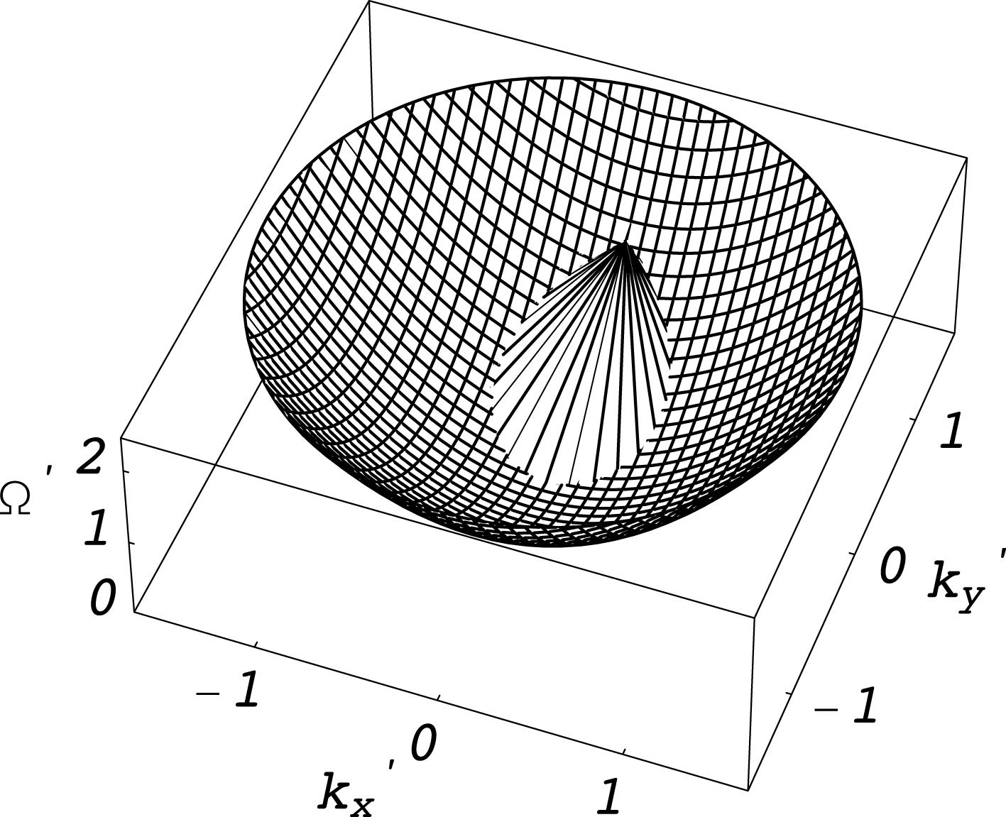
Illustration of the constraints on Langmuir decay imposed by the dispersion relations together with the frequency and wavenumber matching conditions. In the normalized units we have the Langmuir wave dispersion relation to be a parabolic shape
 $\unicode[STIX]{x1D6FA}^{\prime }(k^{\prime })={k^{\prime }}^{2}$
and for the sound wave
 $W^{\prime }=|K^{\prime }|$
as given by the inverted cone. We have
 $k_{0}^{\prime }=1.1$
. The peak of the cone is placed at
 $\unicode[STIX]{x1D6FA}^{\prime }(k_{0}^{\prime })$
.

In three spatial dimensions, the frequency and wavenumber matching conditions impose a restriction on the Langmuir decay (Thornhill & ter Haar Reference Thornhill and ter Haar1978). This has the normalized form
 $$\begin{eqnarray}K^{\prime }=2k_{0}^{\prime }\cos \unicode[STIX]{x1D703}_{2}-1>0,\end{eqnarray}$$
where
 $\unicode[STIX]{x1D703}_{2}$
is the angle between
 $\boldsymbol{K}$
and
 $\boldsymbol{k}_{0}$
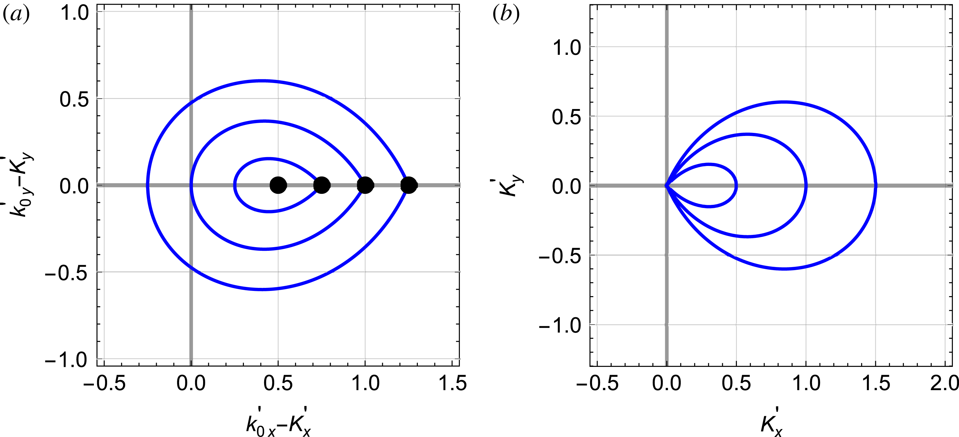
. A multi-dimensional geometrical representation of the Langmuir decay is attempted figures 2 and 3, where figure 2 shows a parabolic Langmuir dispersion relation and an inverted cone representing the sound decay product. The crossing of the two surfaces gives the wavenumber of the Langmuir decay wave. The relative length of the straight line segments give the relative magnitude of the corresponding ion sound wavenumber. An alternative presentation is given in figure 3 showing the ‘daughter Langmuir wave vector’ on a wave vector plane and a similar figure for the sound wave vectors. Given
 $\boldsymbol{k}_{0}$
and
 $E_{0}$
for a plane wave, the problem is completely specified. The wavenumber determines the frequency
 $\unicode[STIX]{x1D714}_{0}$
through the dispersion relation and the selection rule determines the basic sound wave vector
 $\boldsymbol{K}$
and thereby the Langmuir decay product
 $\boldsymbol{k}_{0}-\boldsymbol{K}$
. For a finite wave amplitude we have a finite bandwidth and the choice of available
 $\boldsymbol{K}$
specifies
 $W(\boldsymbol{K})=\text{Re}\{W(\boldsymbol{K})\}+i\text{Im}\{W(\boldsymbol{K})\}$
. For given wave parameters it is thus sufficient to consider
 $\boldsymbol{K}$
(i.e. its magnitude and direction) to determine the decay instability.
(a) shows the wave vector
 $\{k_{0y}^{\prime }-K_{y}^{\prime };k_{0x}^{\prime }-K_{x}^{\prime }\}$
of the decay Langmuir wave with
 $k_{0}^{\prime }$
being along
 $\widehat{\boldsymbol{y}}$
for four cases,
 $k_{0y}^{\prime }=0$
and
 $k_{0x}^{\prime }=0.5,0.75,1.0$
and
 $1.25$
. The limiting case is here
 $k_{0}^{\prime }=1/2$
where the sound speed equals the Langmuir wave group velocity. The small black discs represent the appropriate
 $k_{0}^{\prime }$
. Figure (b) shows the end points of wave vectors of the corresponding decay sound waves. The figures are rotationally symmetric with respect to the horizontal axis for a three-dimensional presentation.

The dispersion relation and the strict wavenumber–frequency matching condition in figures 2 and 3 is found only in the limit of negligible coupling coefficients, i.e. when the right-hand side of (2.6) is infinitesimal and the growth rates of the decay instability are small, giving negligible bandwidths. The finite growth rate for finite amplitudes
 $A_{0}$
in (2.6) gives rise to a line broadening in the dispersion relation that will be illustrated later on. Considering the case with aligned wave vectors
 $\boldsymbol{k}_{0}\Vert \boldsymbol{K}$
we note that we have forward Langmuir wave scattering when
 $1/2<k_{0}^{\prime }\leqslant 1$
and backward scattering for
 $k_{0}^{\prime }>1$
. Starting with a Langmuir wave with
 $1/2<k_{0}^{\prime }\leqslant 3/2$
, we find the decay Langmuir wave product to be stable with respect to decay, but being in the modulationally unstable wavenumber range.
The real and imaginary parts of a numerical solution of (2.2) for a case with Langmuir wave decay is shown in figure 4. We find the growth rate for the decay with the corresponding unstable normalized sound wave vectors
 $\boldsymbol{K}^{\prime }$
. Changing
 $C^{\prime }$
has only little effect on
 $\text{Re}\{W^{\prime }\}$
, but smaller
 $C^{\prime }$
gives a reduction in growth rates
 $\text{Im}\{W^{\prime }\}$
and narrower bandwidths. Note that the contours of the growth rates in figure 4 follow the sound wave contours in figure 3. It is a general feature, also seen in figure 4, that the largest growth rates are found when the wave vectors
 $\boldsymbol{k}_{0},\boldsymbol{K}$
and thereby
 $\boldsymbol{k}_{1}\equiv \boldsymbol{k}_{0}-\boldsymbol{K}$
are aligned (Thornhill & ter Haar Reference Thornhill and ter Haar1978). This observation is often used to justify a one-dimensional model for weakly nonlinear Langmuir waves since such a model captures the dominant contributions.
Numerical solution of the normalized version of (2.2) for
 $k_{0}^{\prime }=1.25$
and
 $C^{\prime }=0.05$
. The growth rate is largest for
 $K_{y}^{\prime }=0$
.

The maximum growth rates of the decay instabilities depend on the initial wave amplitude
 $A_{0}$
: in terms of physical, non-normalized, variables, we can express the maximum growth rate for small wave amplitudes and a given
 $\boldsymbol{k}_{0}$
as (Thornhill & ter Haar Reference Thornhill and ter Haar1978)
 $$\begin{eqnarray}\text{Im}\{W\}\approx \frac{1}{2\sqrt{2}}(k_{0}\unicode[STIX]{x1D706}_{D})^{1/2}\left(\frac{m}{M}\right)^{1/4}\unicode[STIX]{x1D714}_{pe}\sqrt{\frac{\unicode[STIX]{x1D700}_{0}|E_{0}|^{2}}{n_{0}T_{e}}}\sim A_{0},\end{eqnarray}$$
where the implied condition
 $\text{Im}\{W\}\ll \text{Re}\{W\}$
gives here
 $k_{0}\unicode[STIX]{x1D706}_{D}\gg (M/m)^{1/2}\unicode[STIX]{x1D700}_{0}|E_{0}|^{2}/(n_{0}T_{e})$
. In the alternative limit, where the growth rate is comparable to or larger than the sound wave frequency, we find a maximum growth rate
 $$\begin{eqnarray}\text{Im}\{W\}\approx \frac{1}{2^{2/3}}(k_{0}\unicode[STIX]{x1D706}_{D})^{2/3}\left(\frac{m}{M}\right)^{1/3}\unicode[STIX]{x1D714}_{pe}\left(\frac{\unicode[STIX]{x1D700}_{0}|E_{0}|^{2}}{n_{0}T_{e}}\right)^{1/3}\sim A_{0}^{2/3}.\end{eqnarray}$$
The condition
 $\text{Im}\{W\}\gg \text{Re}\{W\}$
gives here
 $k_{0}\unicode[STIX]{x1D706}_{D}\ll (M/m)^{1/2}\unicode[STIX]{x1D700}_{0}|E_{0}|^{2}/(n_{0}T_{e})$
, which has to be satisfied simultaneously with
 $k_{0}>k_{c}$
by (1.4). This latter limit may not be relevant for realistic physical conditions.
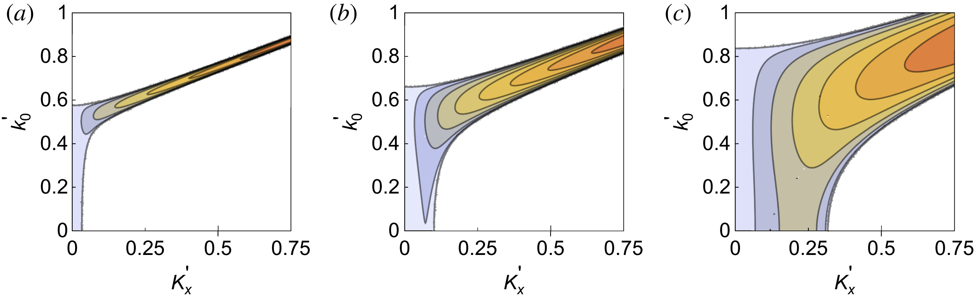
Summary of the variation of the normalized growth rates
 $\text{Im}\{W^{\prime }\}$
for modulational and decay instabilities with varying wave amplitudes and carrier wavenumbers, all assuming
 $\unicode[STIX]{x1D703}=0$
. We have
 $C^{\prime }=0.001,0.01,0.1$
, in (a,b) and (c), respectively. The maximum (i.e. darkest) contours are 0.01, 0.03, and 0.1, with equal spacing between contours in all cases.

Summary plots for the growth rates of modulational and Langmuir decay instabilities are given in figure 5. The figures take
 $\unicode[STIX]{x1D703}=0$
corresponding to
 $\boldsymbol{k}_{0}\Vert \boldsymbol{K}\Vert \boldsymbol{k}_{1}\equiv \boldsymbol{k}_{0}-\boldsymbol{K}$
where the growth rates are largest. In all cases the decay instability, when it is possible, has the largest growth rate that is increasing with
 $k_{0}$
, consistent with (2.9) and (2.10). For small wave amplitudes, i.e. small coupling coefficients
 $C^{\prime }$
, we find a well-defined separation between modulational and decay instabilities as given by
 $k_{c}^{\prime }=1/2$
. As the wave amplitude is increased also the bandwidth increases and the distinction between modulational and decay instabilities becomes blurred even for moderate amplitudes as
 $C^{\prime }=0.1$
. The results of figure 5 also resolves the singularity at the intermediate wavenumber
 $k_{0}^{\prime }=1/2$
separating modulational and decay instabilities: the distinction between the two is smeared out at finite amplitudes where
 $K^{\prime }\approx 0$
can be seen as a modulation as well as a decay product. The wavenumber
 $k_{0}^{\prime }=1/2$
serves as a well-defined separation wavenumber only in the limit of
 $|E_{0}|^{2}\rightarrow 0$
. The strict resonance condition for Langmuir decay,
 $\unicode[STIX]{x1D714}^{(s)}+\unicode[STIX]{x1D714}_{1}^{(\ell )}=\unicode[STIX]{x1D714}_{0}^{(\ell )}$
with
 $\boldsymbol{K}+\boldsymbol{k}_{1}=\boldsymbol{k}_{0}$
, applies only in the limit of infinitesimal wave amplitudes.
Summary figures for the variation of the normalized growth rates
 $\text{Im}\{W^{\prime }\}$
with increasing wave amplitudes
 $C^{\prime }$
for fixed
 $k_{0}^{\prime }=0.75$
and
 $1.25$
, respectively. Both cases assume
 $\unicode[STIX]{x1D703}=0$
. Note that the amplitude range is large on this figure: most of the other cases analysed in this paper refer to small values of
 $C^{\prime }$
since these are most relevant for space applications.

In the basic fluid model (1.1) and (1.2) we find a separation between modulational and decay instabilities at
 $k_{c}$
for small amplitudes, i.e. in the limit where the approximation (2.3) is applicable. Based on a kinetic ion model (Dysthe & Pécseli Reference Dysthe and Pécseli1977; Shatashvili & Tsintsadze Reference Shatashvili and Tsintsadze1982) it was found that nonlinear ion Landau damping makes a wider range of Langmuir wavenumbers (i.e. exceeding
 $k_{c}$
) modulationally unstable.
As a supplement to the information in figure 5 we show in figure 6 two cases for the amplitude variation of the normalized growth rate of the decay instability. We have
 $k_{0}^{\prime }=0.75$
and
 $1.25$
, respectively. In both cases we find that
 $\text{Im}\{W^{\prime }\}\sim \sqrt{C^{\prime }}$
taken at
 $K^{\prime }=2k_{0}^{\prime }-1$
is a good approximation within the range of variation shown, see also (2.9). The increase in bandwidth with increasing
 $C^{\prime }$
can be seen clearly. The bandwidth variation with
 $K^{\prime }$
is not symmetric when
 $C^{\prime }$
is increased, with the asymmetry being most conspicuous for small
 $k_{0}$
.
Kinetic effects such as linear or nonlinear Landau damping of the daughter Langmuir wave and the Landau damping of the ion sound wave decrease the growth rate of the decay instability. The decay instability is primarily controlled by a resonance condition, and effects destroying the resonance, including nonlinear frequency shifts, will reduce the growth rate. Similar effects are found when many waves can participate in widening the resonance and the instability is reduced. The growth rates found in the present paper show no threshold. If a time irreversible damping mechanism is included for the decay Langmuir wave and sound wave, due to for instance collisions between ions and electrons or between plasma particles and neutrals, the growth rate of the decay instability has to compensate for this damping and a threshold amplitude will appear.
3 Two-wave modes
The single-wave-mode case can be generalized to include two or more modes specified by their wavenumbers
 $\boldsymbol{k}_{01}$
and
 $\boldsymbol{k}_{02}$
and relative amplitudes. The analysis giving (1.6) uses an equivalent of the random phase approximation for the steady state unperturbed spectrum, meaning that the relative phase of the two Langmuir modes considered is uniformly distributed over the ensemble. For a one-wave-mode problem the distinction of a random phase is of no concern.
With two waves present, a number of combinations appear: (i) we can have two waves that are individually modulationally unstable, (ii) one wave modulationally unstable and another decay unstable and (iii) two waves both unstable with respect to decay, limiting possibilities being forward and backward scattering. For each of the cases there are infinitely many combinations of
 $\boldsymbol{k}_{01}$
and
 $\boldsymbol{k}_{02}$
and their amplitudes. In particular, the angle between the wave vectors
 $\boldsymbol{k}_{01}$
and
 $\boldsymbol{k}_{02}$
will enter as a parameter. A particularly relevant and easily realizable problem is found when an incoming wave undergoes perfect reflection and we are left with two counter-propagating waves with equal amplitudes and the same wavenumbers. The modulational stability of two such waves was illustrated by Pécseli (Reference Pécseli2014). At that time it was an almost trivial observation that the resulting dispersion relation, the growth rate in particular, was significantly different from the sum of the two individual dispersion relations for the two waves entering the problem. The reason for this is simple: the growth rate for the modulational instability starts at
 $K=0$
and increases for
 $|K|>0$
for either of the two dispersion relations so the two dispersion relations will overlap and the nonlinearity couples the two.
If we start out with one finite-amplitude decay unstable Langmuir wave, the decay products will eventually reach finite amplitudes as well. These waves will be distributed with varying amplitudes along the full lines shown in figure 3(a). The wave component with wave vector aligned with the ‘mother wave’ will however have the largest growth rate, and it will eventually dominate the decay spectrum so that, together with the mother wave, it appears as being composed of two waves only, with aligned wave vectors.
For the case with two waves with one or both being in the decay wavenumber range the conditions differ from the modulationally unstable case. The result becomes particularly complicated when the two wave vectors
 $\boldsymbol{k}_{01}$
and
 $\boldsymbol{k}_{02}$
are oblique.
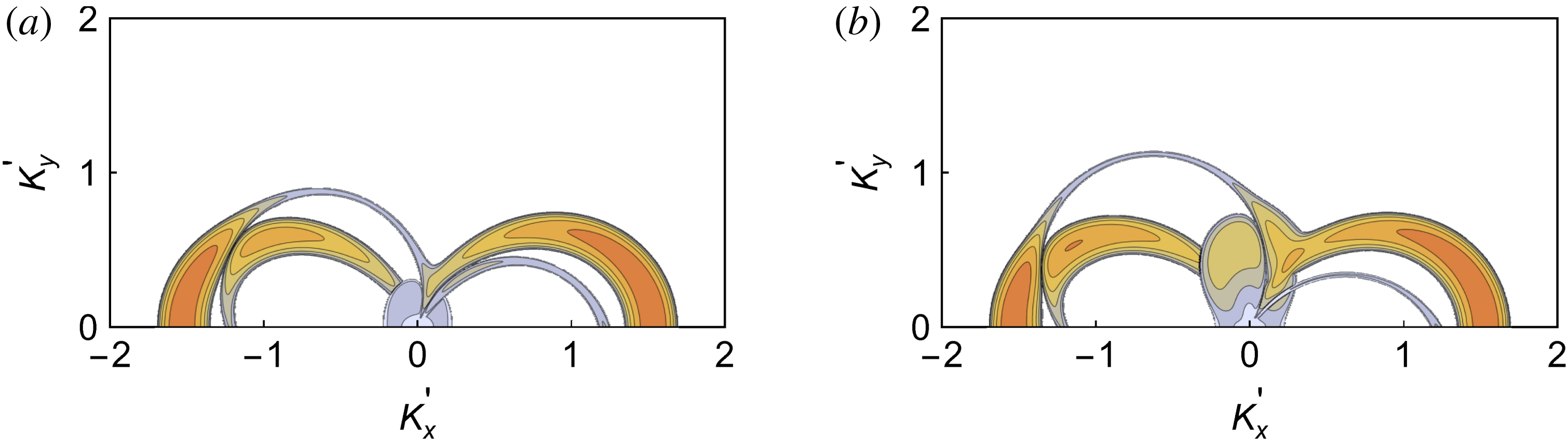
Summary of the normalized growth rates
 $\text{Im}\{W^{\prime }\}$
for the problem with two waves. The case where a wave is in the modulationally unstable condition, the other one decaying with
 $k_{01}^{\prime }=0.4$
and
 $k_{02}^{\prime }=1.25$
, is shown in (a). The case where both are in the Langmuir decay region with
 $k_{01}^{\prime }=0.75$
and
 $k_{02}^{\prime }=1.25$
is shown in (b). The two wave vectors are at right angles in both cases with
 $\boldsymbol{k}_{01}$
vertical. All waves have normalized amplitudes
 $C^{\prime }=0.05$
. The maximum contour level is 0.1 in both cases. A full three-dimensional description in a wave vector space is not presented here, but can be derived by the analysis giving (a) and (b).

The summary in figure 7 illustrates two of the mentioned combinations. In figure 7(a) we have the small growth rate region near
 $K=0$
originating from the modulationally unstable wave, and the broad semi-circular contributions coming from the decay instability. In figure 7(b) we illustrate the ‘competition’ between two decaying Langmuir waves, one giving rise to forward and the other to backward scattered Langmuir waves.
Based on the expression (2.1) with
 $N=2$
and the examples shown in figure 7 we can conclude that two waves with widely separate wavenumbers will interact significantly when their dispersion relations are close. This happens always for
 $K\approx 0$
and there we will find significant deviations from the simple sum of the two decay relations. The important observation is that even for the case where we start out with only two Langmuir waves, the ultimate result will be a distribution of wave energy filling a substantial part of wave vector space.
4 Wide band spectra
A part of the expression (2.6) is recognized also in the denominator of the integral in (1.6). Solving (1.6) for a narrow spectrum we recover the foregoing results, but the expression contains also the more general results for a wide spectrum. In principle we can assume any power spectrum
 $G_{0}(\boldsymbol{k})$
of the Langmuir waves, for instance also some with several local maxima. In practice, it is necessary to make some approximations to the spectra in order to obtain analytically or numerically tractable results (Bhakta & Majumder Reference Bhakta and Majumder1983; Pécseli Reference Pécseli2014). One such approximation assumes a Gaussian spectrum, where the plasma dispersion function can be used, as discussed also in appendix A. Such a spectrum can be specified by the wave power (indicated by
 $A_{0}^{2}$
in appendix A), a central wave vector
 $\boldsymbol{k}_{0}$
(which can be zero) and the spectral width
 $\unicode[STIX]{x1D6E5}$
. For a slightly more general case we can assume anisotropic widths: this case is not considered here.
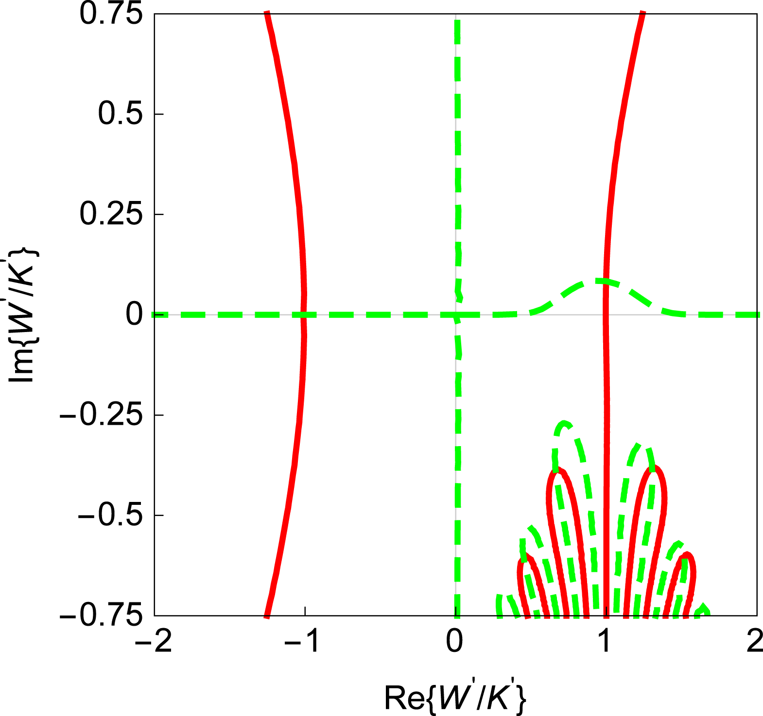
To illustrate some basic features of the solutions for the dispersion relation with a wide Gaussian spectrum we show in figure 8 the complex
 $W^{\prime }/K^{\prime }$
-plane for a selected set of parameters. We find a complex unstable solution with
 $\text{Re}\{W^{\prime }/K^{\prime }\}\approx 1$
, corresponding to the normalized sound velocity. Several damped solutions are also found: these may correspond to the damped sound wave solutions mentioned by Vedenov et al. (Reference Vedenov, Gordeev and Rudakov1967), but since we find unstable solutions, they have comparatively little interest here.
The number of parameters become large and only some selected cases will be illustrated here. We note, for instance, that the maximum growth rates are in all cases found for
 $\boldsymbol{K}\Vert \boldsymbol{k}_{0}\neq 0$
, so only variations with this direction of
 $\boldsymbol{K}$
will be shown.
Illustration of zeroes for the dispersion relation in the complex phase velocity
 $W^{\prime }/K^{\prime }$
-plane. We have
 $k_{0}^{\prime }=1.25$
,
 $K^{\prime }=1.5$
,
 $\unicode[STIX]{x1D6E5}^{\prime }=0.1$
and
 $C^{\prime }=0.1$
. Red lines give zeroes for real part of the dispersion relation, green dashed lines for the imaginary part. Solutions for normalized complex phase velocities
 $W^{\prime }/K^{\prime }$
are found where the two lines cross. The unstable solution has
 $\text{Re}\{W^{\prime }\}/K^{\prime }\approx 1$
in normalized units.

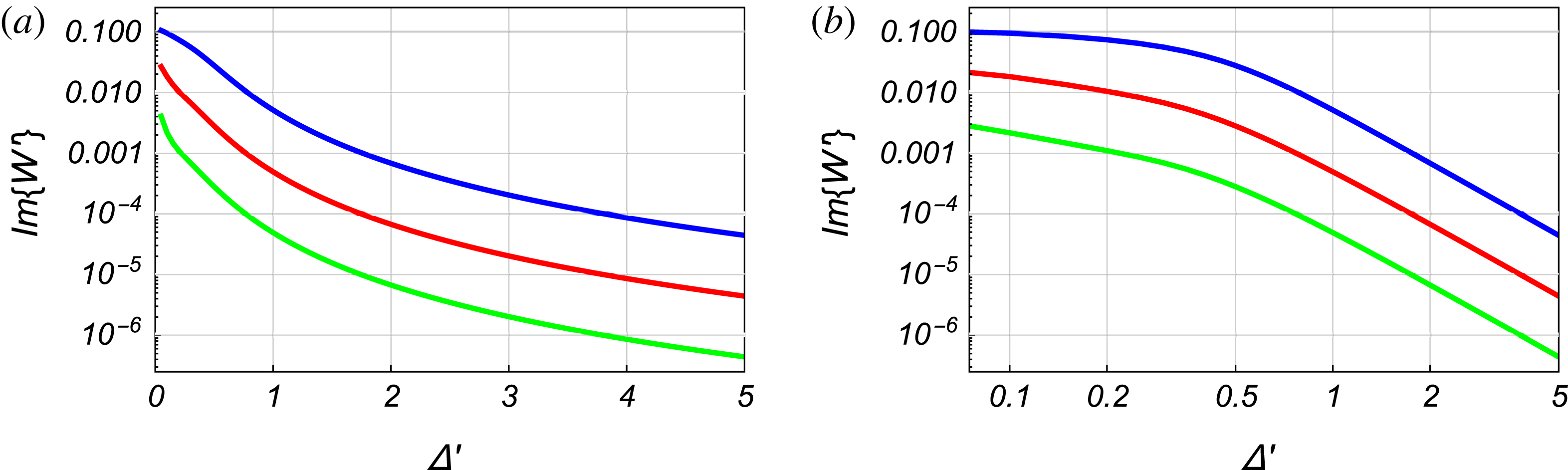
Illustration of the normalized growth rate
 $\text{Im}\{W^{\prime }\}$
as a function of
 $K^{\prime }=2k_{0}^{\prime }-1$
for varying normalized width
 $\unicode[STIX]{x1D6E5}^{\prime }$
of the Langmuir wave spectrum. We have the normalized central wavenumbers of the Gaussian spectrum to be
 $k_{0}^{\prime }=1.25$
(backward scattering,
 $K^{\prime }\approx 1.5$
, see also figure 3) and
 $k_{0}^{\prime }=0.75$
(forward scattering,
 $K^{\prime }\approx 0.5$
) with
 $C^{\prime }=0.005$
in both cases.

4.1 Decay of a wide band spectrum
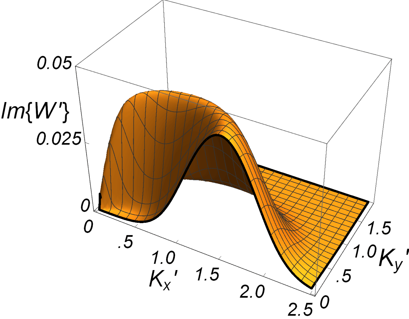
To illustrate results for decay of a Langmuir wave spectrum we have in figure 9(a) a case where the normalized central wave number of the Gaussian spectrum is
 $k_{0}^{\prime }=1.25$
. When the spectrum is narrow,
 $\unicode[STIX]{x1D6E5}^{\prime }\rightarrow 0$
this would correspond to backward scattering, see also figure 3. For
 $\unicode[STIX]{x1D6E5}^{\prime }=0$
we note the finite bandwidth due to finite wave amplitudes found also in, for instance, figure 5. As
 $\unicode[STIX]{x1D6E5}^{\prime }$
increases, the bandwidth is increasing, but the growth rate decreases.
Illustration of the normalized growth rate
 $\text{Im}\{W^{\prime }\}$
with the normalized wavenumber in a
 $(K_{x}^{\prime },K_{y}^{\prime })$
-plane. We have
 $k_{0}^{\prime }=1.25$
along
 $\widehat{\boldsymbol{x}}$
,
 $\unicode[STIX]{x1D6E5}^{\prime }=0.25$
, and
 $C^{\prime }=0.05$
, i.e. a factor 10 increase compared to figure 9.

The variation of the normalized growth rate
 $\text{Im}\{W^{\prime }\}$
with the normalized wavenumber in a
 $(K_{x}^{\prime },K_{y}^{\prime })$
-plane is shown in figure 10 for fixed spectral bandwidth
 $\unicode[STIX]{x1D6E5}^{\prime }=0.25$
. In general we find a reduction in the peak growth rate and also a broadening of
 $\text{Im}\{W^{\prime }\}$
for varying
 $\boldsymbol{K}^{\prime }$
as compared to the narrow band case with the same normalized amplitudes.
While figure 9(a) corresponds to backward Langmuir wave scattering, we show in figures 9(b) and 11 an illustration of forward scattering. To illustrate the growth rate variations with
 $\unicode[STIX]{x1D6E5}^{\prime }$
we show both semi-logarithmic and double logarithmic presentations of the same curves in figure 11. All curves end up having the same
 $\text{Im}\{W^{\prime }\}\sim (\unicode[STIX]{x1D6E5}^{\prime })^{-\unicode[STIX]{x1D6FC}}$
variation for large
 $\unicode[STIX]{x1D6E5}^{\prime }$
with
 $\unicode[STIX]{x1D6FC}\approx 3$
to good accuracy, with
 $\unicode[STIX]{x1D6FC}$
independent of
 $C^{\prime }$
. As
 $k_{0}^{\prime }$
is reduced from the backward scattering limit to smaller forward scattered
 $k_{0}^{\prime }$
, the power-law variations set in for smaller
 $k_{0}^{\prime }$
. Inspection of figure 11 shows that the smallest wave intensities (there with
 $C^{\prime }=0.001$
) are most strongly influenced by an increase in bandwidth. Larger amplitudes, e.g.
 $C^{\prime }=0.1$
in normalized units have almost constant decay rates in a large
 $\unicode[STIX]{x1D6E5}^{\prime }$
interval. By simple intuition it could be argued that for sufficiently wide wavenumber spectra it should not matter whether the central wavenumber corresponds to forward or backward scattering.
Illustration of the normalized growth rate
 $\text{Im}\{W^{\prime }\}$
as a function of the normalized spectral width
 $\unicode[STIX]{x1D6E5}^{\prime }$
for fixed
 $K^{\prime }=0.5$
, corresponding to the maximal growth rate in all three cases. We have the normalized central wavenumber of the Gaussian spectrum to be
 $k_{0}^{\prime }=0.75$
and
 $C^{\prime }=0.1,0.01$
and
 $0.001$
for the three cases shown. Both semi-logarithmic and double logarithmic presentations are shown.

Inspection of the smallest-amplitude case,
 $C^{\prime }=0.001$
in figure 11 shows that there is a characteristic bandwidth where the variation of
 $\text{Im}\{W^{\prime }\}$
with increasing
 $\unicode[STIX]{x1D6E5}^{\prime }$
changes from one power law to a steeper
 $\text{Im}\{W^{\prime }\}\sim (\unicode[STIX]{x1D6E5}^{\prime })^{-3}$
power-law variation. It is found that the asymptotic variation is the same for all
 $C^{\prime }$
and
 $k_{0}^{\prime }$
studied, but the transition bandwidth varies.
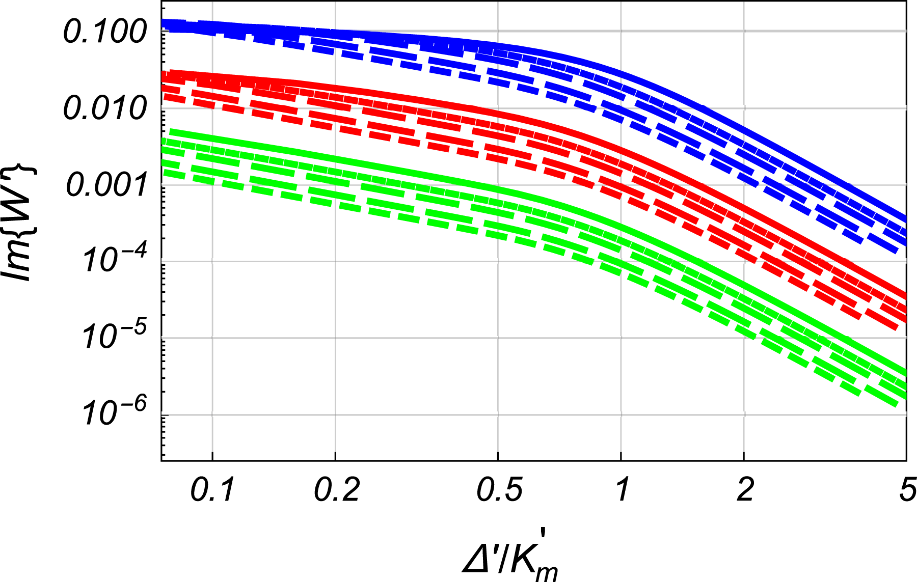
To understand the role of the transition bandwidth we show in figure 12 a compensated variation as a function of
 $\unicode[STIX]{x1D6E5}^{\prime }/K_{m}^{\prime }$
where for each set of curves
 $K_{m}^{\prime }=2k_{0}^{\prime }-1$
corresponds to the wavenumber
 $K^{\prime }$
having the largest growth rate
 $\text{Im}\{W^{\prime }\}$
for the given
 $k_{0}^{\prime }$
. There is no natural growth rate to use for compensation of
 $\text{Im}\{W^{\prime }\}$
, so the ordinate is not compensated. In this compensated representation we find that the change from a
 $\text{Im}\{W^{\prime }\}\sim (\unicode[STIX]{x1D6E5}^{\prime })^{-1}$
variation to
 $\text{Im}\{W^{\prime }\}\sim (\unicode[STIX]{x1D6E5}^{\prime })^{-3}$
happens when
 $\unicode[STIX]{x1D6E5}^{\prime }/K_{m}^{\prime }\approx 1$
in all cases. Physically, this observation is consistent with an interpretation where an increase in wavenumber bandwidth of the Langmuir wave spectrum gives a reduction in decay rate. For constant small
 $C^{\prime }$
and varying
 $\unicode[STIX]{x1D6E5}^{\prime }$
the reduction follows a power law
 ${\sim}(\unicode[STIX]{x1D6E5}^{\prime })^{-1}$
. The simple ‘independence assumption’ mentioned in the Introduction would give a decrease for
 $\text{Im}\{W^{\prime }\}$
as
 $(\unicode[STIX]{x1D6E5}^{\prime })^{-1/2}$
for small wave energy densities and
 $(\unicode[STIX]{x1D6E5}^{\prime })^{-1/3}$
for larger energy densities according to (2.9) and (2.10). The ‘independence assumption’ is at variance with our results.
As an estimate we can assume that the correlation length associated with the power spectrum is
 ${\sim}(\unicode[STIX]{x1D6E5}^{\prime })^{-1}$
. A transition is found when this correlation length becomes comparable to the wavelength
 ${\sim}(K^{\prime })^{-1}$
of the sound wave with maximum decay rate for the given
 $k_{0}^{\prime }$
. In this case the decay becomes impeded and a further increase in bandwidth (reduction in correlation length) gives a correspondingly stronger reduction in the growth rate
 $\text{Im}\{W^{\prime }\}$
. The growth rate is reduced, but the decay is not completely inhibited. A reduction in the decay rate of, say, a factor of 100 is, however, close to stabilization for most practical cases.
Illustration of the normalized growth rate
 $\text{Im}\{W^{\prime }\}$
as a function of the compensated spectral width
 $\unicode[STIX]{x1D6E5}^{\prime }/K_{m}^{\prime }$
for
 $K_{m}^{\prime }$
corresponding to the maximal growth rate in all cases. We have the normalized central wavenumber of the Gaussian spectrum to be
 $k_{0}^{\prime }=3/4,7/8,1,5/4,3/2$
and
 $C^{\prime }=0.1,0.01$
and
 $0.001$
for the cases shown. Note that the growth rate
 $\text{Im}\{W^{\prime }\}$
has not been compensated.

The present subsection addresses spectra where the central peak amplitude wave mode is for
 $k_{0}^{\prime }>1/2\equiv k_{c}^{\prime }$
, i.e. in the decay range. Reducing
 $k_{0}^{\prime }$
we find a transition region near
 $k_{0}^{\prime }\approx 1/2$
: for
 $k_{0}^{\prime }<k_{c}^{\prime }$
the reduction of
 $\text{Im}\{W^{\prime }\}$
with increasing
 $\unicode[STIX]{x1D6E5}^{\prime }$
becomes even more pronounced. We here recover the results shown by Pécseli (Reference Pécseli2014) where the reduction in
 $\text{Im}\{W^{\prime }\}$
is faster than exponential for increasing
 $\unicode[STIX]{x1D6E5}^{\prime }$
. Details of the transition region depend on the energy density of the power spectrum
 $G_{0}(\boldsymbol{k})$
.
4.2 A plane wave propagating in a background of a wide band spectrum
The general expression (1.6) allows the spectrum
 $G_{0}(\boldsymbol{k})$
to be composed of several Gaussian forms where each can be modelled via the plasma dispersion function. Strongly anisotropic wave spectra can be modelled easily by such an approach.
In particular we can by (1.6) also model the propagation of a single-wave mode in a background of low level Langmuir turbulence. The general result relevant here can be obtained by inserting
 $G_{0}(\boldsymbol{k})=A^{2}\,\unicode[STIX]{x1D6FF}(\boldsymbol{k}-\boldsymbol{k}_{0})+G_{\unicode[STIX]{x1D6FC}}(\boldsymbol{k})$
into (1.6), where
 $G_{\unicode[STIX]{x1D6FC}}(\boldsymbol{k})$
denotes the power spectrum of the background Langmuir waves. Restricting the problem to one spatial dimension with
 $\boldsymbol{K}\Vert \boldsymbol{k}_{0}$
we find
 $$\begin{eqnarray}\displaystyle & & \displaystyle (W+C_{s}K)(W-C_{s}K)\left(W-\frac{\unicode[STIX]{x1D710}^{2}}{\unicode[STIX]{x1D714}_{pe}}k_{0}K+\frac{1}{2}\frac{\unicode[STIX]{x1D710}^{2}}{\unicode[STIX]{x1D714}_{pe}}K^{2}\right)\nonumber\\ \displaystyle & & \displaystyle \quad =\frac{\unicode[STIX]{x1D700}_{0}\unicode[STIX]{x1D710}^{2}K^{4}}{8Mn_{0}}\,\frac{A^{2}}{\left(W-\displaystyle \frac{\unicode[STIX]{x1D710}^{2}}{\unicode[STIX]{x1D714}_{pe}}k_{0}K-\frac{1}{2}\frac{\unicode[STIX]{x1D710}^{2}}{\unicode[STIX]{x1D714}_{pe}}K^{2}\right)}+\left(W-\frac{\unicode[STIX]{x1D710}^{2}}{\unicode[STIX]{x1D714}_{pe}}k_{0}K+\frac{1}{2}\frac{\unicode[STIX]{x1D710}^{2}}{\unicode[STIX]{x1D714}_{pe}}K^{2}\right)\frac{\unicode[STIX]{x1D700}_{0}\unicode[STIX]{x1D710}^{2}K^{4}}{8Mn_{0}}\nonumber\\ \displaystyle & & \displaystyle \qquad \times \,\int _{-\infty }^{\infty }\frac{G_{\unicode[STIX]{x1D6FC}}(\unicode[STIX]{x1D705})}{\left(W-\displaystyle \frac{\unicode[STIX]{x1D710}^{2}}{\unicode[STIX]{x1D714}_{pe}}\unicode[STIX]{x1D705}K\right)^{2}-\left(\displaystyle \frac{1}{2}\frac{\unicode[STIX]{x1D710}^{2}}{\unicode[STIX]{x1D714}_{pe}}K^{2}\right)^{2}}\,\text{d}\unicode[STIX]{x1D705},\end{eqnarray}$$
where the integral, with parts of its coefficient included, can be written as
 $$\begin{eqnarray}\displaystyle & & \displaystyle \frac{\unicode[STIX]{x1D710}^{2}K^{2}}{\unicode[STIX]{x1D714}_{pe}}\int _{-\infty }^{\infty }\frac{G_{\unicode[STIX]{x1D6FC}}(\unicode[STIX]{x1D705})}{\left(W-\displaystyle \frac{\unicode[STIX]{x1D710}^{2}}{\unicode[STIX]{x1D714}_{pe}}\unicode[STIX]{x1D705}K\right)^{2}-\left(\displaystyle \frac{1}{2}\frac{\unicode[STIX]{x1D710}^{2}}{\unicode[STIX]{x1D714}_{pe}}K^{2}\right)^{2}}\,\text{d}\unicode[STIX]{x1D705}\nonumber\\ \displaystyle & & \displaystyle \quad =\int _{-\infty }^{\infty }\frac{G_{\unicode[STIX]{x1D6FC}}(\unicode[STIX]{x1D705})}{W-\displaystyle \frac{\unicode[STIX]{x1D710}^{2}}{\unicode[STIX]{x1D714}_{pe}}\unicode[STIX]{x1D705}K-\frac{1}{2}\frac{\unicode[STIX]{x1D710}^{2}}{\unicode[STIX]{x1D714}_{pe}}K^{2}}\,\text{d}\unicode[STIX]{x1D705}-\int _{-\infty }^{\infty }\frac{G_{\unicode[STIX]{x1D6FC}}(\unicode[STIX]{x1D705})}{W-\displaystyle \frac{\unicode[STIX]{x1D710}^{2}}{\unicode[STIX]{x1D714}_{pe}}\unicode[STIX]{x1D705}K+\frac{1}{2}\frac{\unicode[STIX]{x1D710}^{2}}{\unicode[STIX]{x1D714}_{pe}}K^{2}}\,\text{d}\unicode[STIX]{x1D705}.\end{eqnarray}$$
Only minor modifications of the wave characteristics are found for the case where a large-amplitude narrow band mode is propagated in a plasma where a low level, broad band electron plasma wave spectrum is excited. This result agrees with intuitive expectations. The conditions could be different for the case where a small-amplitude test wave propagates in a background of large-amplitude, wide band Langmuir wave turbulence. It turns out, however, that also in this latter case the dynamics, decay in particular, of the narrow band wave is largely unaffected. The reason is that only the energy content of the waves with wave vectors close to
 $\boldsymbol{k}_{0}$
seem to matter, and if the spectral wave energy is distributed over a wide wavenumber range, the energy density in wavenumber space will generally be small everywhere.
Qualitatively, the results can be understood by inspecting (4.1) and (4.2). To lowest approximation for small amplitudes
 $A$
we have
 $\text{Im}\{W\}\ll \text{Re}\{W\}$
and
 $\text{Re}\{W\}\pm C_{s}K\approx 0$
, giving
 $W^{2}-C_{s}^{2}K^{2}\approx i2C_{s}K\,\text{Im}\{W\}$
. At the same time
 $\text{Re}\{W\}-(\unicode[STIX]{x1D710}^{2}/\unicode[STIX]{x1D714}_{pe})k_{0}K+(1/2)(\unicode[STIX]{x1D710}^{2}/\unicode[STIX]{x1D714}_{pe})K^{2}\approx 0$
for the Langmuir waves. The left-hand side of (4.1) will then be of order
 $\text{Im}\{W\}^{2}$
. The denominator of the first term on the right-hand side of (4.1) is
 $i\text{Im}\{W\}-K^{2}\unicode[STIX]{x1D710}^{2}/\unicode[STIX]{x1D714}_{pe}$
which will remain finite. The parenthesis in the coefficient for the integral in (4.1) is small when the resonance condition is fulfilled and the term can become significant only if the denominator in the integral is small at the same time. Writing the integral in two parts as in (4.2) we find that the denominator of the first part will be of order
 $i\text{Im}\{W\}-(K-k_{0}+\unicode[STIX]{x1D705})K\unicode[STIX]{x1D710}^{2}/\unicode[STIX]{x1D714}_{pe}$
which can become small for
 $\unicode[STIX]{x1D705}\approx k_{0}-K$
. This term can contribute if
 $G_{\unicode[STIX]{x1D6FC}}(\unicode[STIX]{x1D705}\approx k_{0}-K)$
is of significant magnitude. The denominator of the second integral is
 $i\text{Im}\{W\}+(k_{0}-\unicode[STIX]{x1D705})K\unicode[STIX]{x1D710}^{2}/\unicode[STIX]{x1D714}_{pe}$
giving a singularity at
 $\unicode[STIX]{x1D705}\approx k_{0}$
with the contour of integration determined by
 $i\text{Im}\{W\}$
. The second term in (4.2) can reach significant values provided
 $G_{\unicode[STIX]{x1D6FC}}(\unicode[STIX]{x1D705}\approx k_{0})$
has a significant value. Here
 $k_{0}$
is the wavenumber of the initial plane Langmuir wave, and
 $k_{0}-K$
the wavenumber of the decay Langmuir wave: the decay rate depends in general on the value of
 $G_{\unicode[STIX]{x1D6FC}}(\unicode[STIX]{x1D705})$
at both. It is important not to be misguided by the corresponding plasma kinetic Landau analysis: the local derivative of
 $G_{\unicode[STIX]{x1D6FC}}(\unicode[STIX]{x1D705})$
near
 $k_{0}$
or
 $k_{0}-K$
is of no consequence.
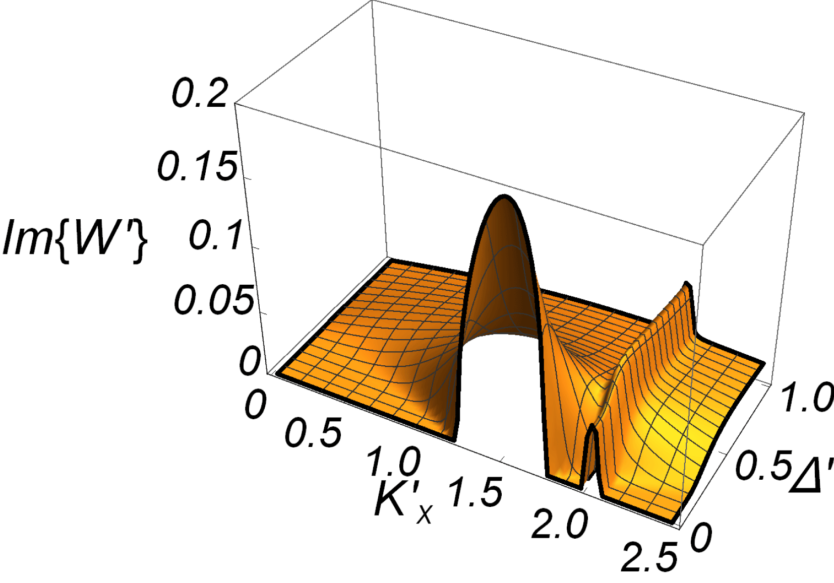
As an illustration we show in figure 13 results for a small-amplitude wave with wavenumber
 $k_{01}$
propagating in a background of enhanced wide band Langmuir wave fluctuations. The small narrow peak at
 $K^{\prime }=2$
marks the decay product of the small-amplitude decaying test wave with
 $k_{01}=1.5$
with constant width and amplitude, while the line broadened decay product at
 $K^{\prime }=1.5$
represents the decaying large-amplitude wave with carrier wavenumber
 $k_{0}=1.25$
where the bandwidth
 $\unicode[STIX]{x1D6E5}^{\prime }$
is increased. At close scrutiny we find a small reduction in decay rate (i.e. a tendency towards stabilization) of the small-amplitude test wave as long as the local Langmuir turbulence level is noticeable, but as soon as the wave spectrum is spread out for enhanced
 $\unicode[STIX]{x1D6E5}^{\prime }$
, the decay rate approaches its value in the absence of any background turbulence. In order to see a stronger interaction for waves propagating in the same direction, the test wave has to be closer to the carrier wavenumber of the turbulence.
Illustration of the normalized growth rate
 $\text{Im}\{W^{\prime }\}$
as a function of the compensated spectral width
 $\unicode[STIX]{x1D6E5}^{\prime }$
and
 $K_{m}^{\prime }$
, obtained for the parameters
 $k_{01}^{\prime }=1.5$
,
 $k_{0}^{\prime }=1.25$
,
 $C^{\prime }=0.1$
,
 $(A^{\prime })^{2}=0.005$
.

5 Conclusion
The analysis summarized in the present work assumes homogeneous plasma conditions. Formally the results can be generalized to inhomogeneous conditions as well, since
 $\widetilde{n}$
in (1.1) can be added any large-scale plasma density variation (Chen & Liu Reference Chen and Liu1978). Other studies (Kontar & Pécseli Reference Kontar and Pécseli2002) indicated that such effects can be important. Damping effects can in principle be incorporated as well, as have been included in the nonlinear Schrödinger equation (Pereira & Stenflo Reference Pereira and Stenflo1977). It is a non-trivial restriction that the basic model assumes a thermal plasma with only one temperature. Multi-temperature plasmas have been studied in the literature and the effects of the so-called electron acoustic waves (Watanabe & Taniuti Reference Watanabe and Taniuti1977; Gary & Tokar Reference Gary and Tokar1985) have been included in some nonlinear models (Khirseli & Tsintsadze Reference Khirseli and Tsintsadze1980; Hanssen et al.
Reference Hanssen, Pécseli, Stenflo and Trulsen1994). These features open a decay channel (Skjaeraasen et al.
Reference Skjæraasen, Krane, Pécseli, Stenflo and Trulsen1996) in addition to the one studied in the present work but the full consequences of this modification are not well known. The effects of a weak homogeneous magnetic field have been considered by the authors and these results will be reported later. The present analysis considered only electrostatic waves. Since the electrostatic Langmuir branch merges with the electromagnetic branch of the dispersion relation, the two wave forms can couple when the spectrum includes small wavenumbers (Kuznetsov Reference Kuznetsov1974; Thornhill & ter Haar Reference Thornhill and ter Haar1978). To account for this effect to lowest order we include a term
 $-1/2(c^{2}/\unicode[STIX]{x1D714}_{pe})\unicode[STIX]{x1D735}\times \unicode[STIX]{x1D735}\times \boldsymbol{E}$
on the left-hand side of (1.1). As this term is linear it gives a relatively modest additional complexity to the analysis, although the dispersion relation becomes more involved. The constraint
 $\unicode[STIX]{x1D735}\times (\boldsymbol{E}\,\widetilde{n}/n_{0})\approx 0$
mentioned earlier will no longer apply.
The main result from the present studies is a demonstration of a reduction in decay rate of Langmuir wave spectra when their wavenumber spectral bandwidth is increased. The decay rate does not vanish completely but is reduced considerably, indicating that wide band spectra will be observable for a long time, even though they cover a wavenumber range including also decaying wavenumbers with
 $k>k_{c}$
given by (1.4). We can give a qualitative discussion of the decay of a narrow Langmuir wave spectrum, where the bandwidth is smaller than the carrier wavelength,
 $k_{0}\gg k_{c}$
. In this case we have the decay sound wavenumber to be smaller than the bandwidth of the Langmuir wavenumber spectrum,
 $K\ll \unicode[STIX]{x1D6E5}_{k}$
, and the back scatter decay begins as for a plane wave. The amplitude of the decay products increase and a secondary decay begins (the ‘Langmuir cascade’), etc. The excited sound waves will have increasing wavelengths to eventually exceed the correlation length
 $\unicode[STIX]{x1D6E5}_{k}^{-1}$
associated with the original spectrum, and the cascade becomes strongly delayed. This behaviour was actually observed in numerical simulations of ionospheric Langmuir turbulence (Hanssen et al.
Reference Hanssen, Mjølhus, Dubois and Rose1992).
The aim of the present study differs from what is usually called weak turbulence theory (Kadomtsev Reference Kadomtsev1965) where a self-consistent model for the generation and nonlinear evolution of the Langmuir wave spectrum is found, with emphasis on the evolution of the particle velocity distribution function for both the background plasma and for the electron beam that excites the fluctuations (Kontar, Lapshin & Mel’nik Reference Kontar, Lapshin and Mel’nik1998). As with other works (Alber Reference Alber1978), the present analysis is based on a version of the quasi-normal approximation, where averages of some higher-order products are approximated by products of averages (Pécseli Reference Pécseli2014). The most important consequence of the approximation lies in the statistical relations between Fourier components. In all cases we have that two Fourier components for different frequencies or wavenumbers are uncorrelated. If the process is Gaussian, then they are also statistically independent, which is a non-trivial constraint. The full implications of the quasi-normal approximation made in the present context are not known, and a study based on direct numerical simulations of the basic equations would be worthwhile.
The present analysis has a restricted aim: it assumes the Langmuir waves to be given and studies some (but not all) of the basic nonlinear wave phenomena accounted for by (1.1) and (1.2). The turbulence can be generated by a plasma instability with examples given before, or simply by waves originating from some coherent source followed by some mechanism (Dysthe, Pécseli & Trulsen Reference Dysthe, Pécseli and Trulsen1983) that gives rise to a line broadening. Extreme nonlinear phenomena like Langmuir wave collapse (Zakharov Reference Zakharov1972; Rasmussen & Rypdal Reference Rasmussen and Rypdal1986) were not addressed here. Langmuir waves can be important for electron acceleration (Kontar, Ratcliffe & Bian Reference Kontar, Ratcliffe and Bian2012) but also such kinetic plasma effects are left out here.
Langmuir waves are easily excited in a laboratory, although most of these studies relate to magnetized plasmas. The waves can also be excited by ionospheric modification experiments (Perkins, Oberman & Valeo Reference Perkins, Oberman and Valeo1974; Fejer Reference Fejer1979), where in particular, wave decay was observed. The interest for Langmuir wave decay in the ionosphere was revived by the observation of naturally enhanced ion-acoustic lines that are detected in the polar regions (Isham et al. Reference Isham, Rietveld, Guio, Forme, Grydeland and Mjølhus2012) with radar beams nearly aligned with the magnetic field lines. As one possible explanation of the non-thermal ion spectra it has been argued by Forme (Reference Forme1999) that they can be generated by decay of Langmuir waves excited by fast magnetic field aligned electron beams. Authoritative numerical studies of this problem (Guio & Forme Reference Guio and Forme2006; Isham et al. Reference Isham, Rietveld, Guio, Forme, Grydeland and Mjølhus2012; Krafft, Volokitin & Krasnoselskikh Reference Krafft, Volokitin and Krasnoselskikh2015) use basic equations as those discussed in the introduction and include a source term accounting for an electron beam that generates an enhanced level of Langmuir waves.
It may be worth noting that the results summarized in the present work for decay of waves with a wide band turbulent spectrum have a completely different structure than found in related studies by Zakharov (Reference Zakharov1965a ,Reference Zakharov b ) or Sagdeev & Galeev (Reference Sagdeev and Galeev1969). The result (1.6) is also universal in the sense that it allows unified treatment of modulational and decay instabilities of a Langmuir wave spectrum, so the two processes and their interplay can be studied at the same time. A model for Langmuir wave decay of a turbulent spectrum was presented by Edney & Robinson (Reference Edney and Robinson2001). The scope of their analysis was more restrictive than the one presented here. Early models for turbulent spectra, as reviewed by Mima & Nishikawa (Reference Mima, Nishikawa, Galeev and Sudan1984), used a reference wave (sometimes only a diploar electric field) with randomly varying amplitude and phase. We believe our model to be more general.
A wave kinetic equation can be derived by semi-heuristic arguments (Vedenov & Rudakov Reference Vedenov and Rudakov1965; Vedenov et al.
Reference Vedenov, Gordeev and Rudakov1967; Hasegawa Reference Hasegawa1975; Breizman & Malkin Reference Breizman and Malkin1980), with some earlier related studies by Camac et al. (Reference Camac, Kantrowitz, Litvak, Patrick and Petschek1962). A similar model was studied also by Shukla, Stenflo & Faria (Reference Shukla, Stenflo and Faria1998) for weakly collisional plasmas. In these and similar models a wave power spectrum is representing an ensemble of propagating non-dispersive wave packets. The basic equations giving (1.6) contains such a wave kinetic equation as limiting case where the model has the form of a Vlasov equation for quasi-particles (Pécseli Reference Pécseli2014). That model is not reproducing Langmuir decay and to obtain (1.6) it is necessary to allow for propagation and also the dispersion of wave packets accounted for by the
 $(1/2)K^{2}\unicode[STIX]{x1D710}^{2}/\unicode[STIX]{x1D714}_{pe}$
term in the denominator of (1.6). The wave kinetic equation admits a simplified analysis of the modulational instability also by allowing its similarity with the Vlasov equation to be used in numerical models (Tappert & Cole Reference Tappert and Cole1971; Pécseli & Trulsen Reference Pécseli and Trulsen1990; Pécseli & Trulsen Reference Pécseli and Trulsen1992).
The range of validity of the basic equations (1.1) and (1.2) deserve some scrutiny. They are derived by using the square root of the electron-to-ion mass ratio
 $(m/M)^{1/2}$
as a small expansion parameter as also indicated by the normalizations used in § 2. We find that the wavenumber–frequency range for the modulational instability with
 $K<(m/M)^{1/2}/\unicode[STIX]{x1D706}_{De}$
where
 $W<\unicode[STIX]{x1D6FA}_{pi}(m/M)^{1/2}$
is safely within the range of validity of the parameter expansion for wave energy densities
 $(1/2)\unicode[STIX]{x1D700}_{0}A_{0}^{2}<(m/M)n_{0}T_{e}$
, ignoring some numerical factors of order unity. The forward decay instability is marginally within this range, while strictly speaking the backward decay falls outside. A more detailed study, expanding the range of validity of (1.1) and (1.2) by including higher-order terms, would be worthwhile.
Acknowledgements
One of the authors (H.L.P.) thanks K. B. Dysthe, E. Kontar, L. Stenflo and J. K. Trulsen for valuable discussions. This author acknowledges also the kind encouragement and financial support from the Norwegian Space Centre.
Appendix A
The paper by Pécseli (Reference Pécseli2014) had the ambition of deriving a general formalism that in a systematic way could be reduced to contain also the wave kinetic equation of e.g. Vedenov & Rudakov (Reference Vedenov and Rudakov1965), Vedenov et al. (Reference Vedenov, Gordeev and Rudakov1967). The dispersion relations (1.5) or (1.6) can be derived in a simpler way, as outlined here. The analysis can be generalized to other wave types as well.
Starting with the Zakharov equations (1.1) and (1.2) the space–time varying fluctuations in plasma density
 ${\tilde{n}}$
and electric fields
 $\boldsymbol{E}$
are Fourier transformed to give
 ${\tilde{n}}(\boldsymbol{K},W)$
and
 $\boldsymbol{E}(\boldsymbol{K},W)$
where
 $W$
denotes the frequency of the slow time variation. The wave vector of the perturbation is denoted by
 $\boldsymbol{K}$
. The frequency–wavenumber variations of the unmodulated reference Langmuir wave power spectrum are given through
 $(\unicode[STIX]{x1D6FA},\boldsymbol{k})$
. Variations on the fast plasma frequency scale
 $\unicode[STIX]{x1D714}_{pe}$
are removed. In terms of the Fourier transformed quantities we find from (1.1) and (1.2)
 $$\begin{eqnarray}\displaystyle & \hspace{-10.00002pt}\displaystyle \left(W-\frac{K^{2}\unicode[STIX]{x1D710}^{2}}{2\unicode[STIX]{x1D714}_{pe}}\right)\boldsymbol{E}(\boldsymbol{K},W)=\frac{\unicode[STIX]{x1D714}_{pe}}{2}\int \text{d}\boldsymbol{k}_{1}\int \text{d}\unicode[STIX]{x1D6FA}_{1}\frac{{\tilde{n}}(\boldsymbol{k}_{1},\unicode[STIX]{x1D6FA}_{1})}{n_{0}}\boldsymbol{E}(\boldsymbol{K}-\boldsymbol{k}_{1},W-\unicode[STIX]{x1D6FA}_{1}), & \displaystyle\end{eqnarray}$$
 $$\begin{eqnarray}\displaystyle & \hspace{-10.00002pt}\displaystyle (W^{2}-K^{2}C_{s}^{2})\frac{{\tilde{n}}(\boldsymbol{K},W)}{n_{0}}=\frac{\unicode[STIX]{x1D700}_{0}K^{2}}{2Mn_{0}}\int \text{d}\boldsymbol{k}_{1}\!\int \text{d}\unicode[STIX]{x1D6FA}_{1}\,\boldsymbol{E}(\boldsymbol{k}_{1},\unicode[STIX]{x1D6FA}_{1})\boldsymbol{\cdot }\boldsymbol{E}^{\ast }(\boldsymbol{k}_{1}-\boldsymbol{K},\unicode[STIX]{x1D6FA}_{1}-W), & \displaystyle\end{eqnarray}$$
where we used the relation for Fourier transforms in the form
 $F(\unicode[STIX]{x1D705})=\!\int \!F(x)\exp (-\text{i}\unicode[STIX]{x1D705}x)\,\text{d}x$
,
 $F^{\ast }(\unicode[STIX]{x1D705})=\int F^{\ast }(x)\exp (\text{i}\unicode[STIX]{x1D705}x)\,\text{d}x$
and
 $F^{\ast }(-\unicode[STIX]{x1D705})=\int F^{\ast }(x)\exp (-\text{i}\unicode[STIX]{x1D705}x)\,\text{d}x$
. The integrations over
 $\unicode[STIX]{x1D6FA}_{1}$
and
 $\boldsymbol{k}_{1}$
in (A 1) and (A 2) originate from the convolutions in the Fourier transforms of
 $\widetilde{n}E$
and
 $|E|^{2}$
. We use here the short hand notation
 $\int \text{d}\boldsymbol{k}\equiv \int \!\!\int \!\!\int \text{d}k_{x}\,\text{d}k_{y}\,\text{d}k_{z}$
and throughout include a divisor of
 $2\unicode[STIX]{x03C0}$
from each Fourier integration into the transformed function.
For later use we introduce a spectral function
 $G(\boldsymbol{k}_{1}-\boldsymbol{k}/2,\unicode[STIX]{x1D6FA}_{1}-\unicode[STIX]{x1D6FA}/2;\boldsymbol{k},\unicode[STIX]{x1D6FA})$
through the following definition containing an ensemble average given by angular brackets
 $$\begin{eqnarray}\displaystyle & & \displaystyle \int \text{d}\boldsymbol{k}_{1}\!\!\int \text{d}\boldsymbol{k}_{2}\!\int \!\text{d}\unicode[STIX]{x1D6FA}_{1}\!\!\int \!\text{d}\unicode[STIX]{x1D6FA}_{2}\langle \boldsymbol{E}(\boldsymbol{k}_{1},\unicode[STIX]{x1D6FA}_{1})\boldsymbol{\cdot }\boldsymbol{E}^{\ast }(\boldsymbol{k}_{2},\unicode[STIX]{x1D6FA}_{2})\rangle \text{e}^{\text{i}[(\boldsymbol{k}_{1}-\boldsymbol{k}_{2})\boldsymbol{\cdot }\boldsymbol{r}-(\unicode[STIX]{x1D6FA}_{1}-\unicode[STIX]{x1D6FA}_{2})t]}\nonumber\\ \displaystyle & & \displaystyle \quad \equiv \int \!\text{d}\boldsymbol{k}_{1}\!\!\int \!\text{d}\boldsymbol{k}_{2}\int \!\text{d}\unicode[STIX]{x1D6FA}_{1}\int \!\text{d}\unicode[STIX]{x1D6FA}_{2}\,\nonumber\\ \displaystyle & & \displaystyle \qquad \times \,G\left(\frac{\boldsymbol{k}_{1}+\boldsymbol{k}_{2}}{2},\frac{\unicode[STIX]{x1D6FA}_{1}+\unicode[STIX]{x1D6FA}_{2}}{2};\boldsymbol{k}_{1}-\boldsymbol{k}_{2},\unicode[STIX]{x1D6FA}_{1}-\unicode[STIX]{x1D6FA}_{2}\right)\,\text{e}^{\text{i}[(\boldsymbol{k}_{1}-\boldsymbol{k}_{2})\boldsymbol{\cdot }\boldsymbol{r}-(\unicode[STIX]{x1D6FA}_{1}-\unicode[STIX]{x1D6FA}_{2})t]}\nonumber\\ \displaystyle & & \displaystyle \quad =\int \!\!\text{d}\boldsymbol{k}\int \!\!\text{d}\unicode[STIX]{x1D6FA}\left\{\!\!\int \text{d}\boldsymbol{k}_{1}\!\!\int \text{d}\unicode[STIX]{x1D6FA}_{1}\;G\left(\boldsymbol{k}_{1}-\frac{\boldsymbol{k}}{2},\unicode[STIX]{x1D6FA}_{1}-\frac{\unicode[STIX]{x1D6FA}}{2};\boldsymbol{k},\unicode[STIX]{x1D6FA}\right)\right\}\text{e}^{\text{i}(\boldsymbol{k}\boldsymbol{\cdot }\boldsymbol{r}-\unicode[STIX]{x1D6FA}t)}.\end{eqnarray}$$
In the derivation we at one point introduced separation variables in
 $\langle \boldsymbol{E}(\boldsymbol{k}_{1},\unicode[STIX]{x1D6FA}_{1})\boldsymbol{\cdot }\boldsymbol{E}^{\ast }(\boldsymbol{k}_{2},\unicode[STIX]{x1D6FA}_{2})\rangle$
. We then expand
 $G$
as follows
 $$\begin{eqnarray}\displaystyle & & \displaystyle G\left(\boldsymbol{k}_{1}-\frac{\boldsymbol{k}}{2},\unicode[STIX]{x1D6FA}_{1}-\frac{\unicode[STIX]{x1D6FA}}{2};\boldsymbol{k},\unicode[STIX]{x1D6FA}\right)\nonumber\\ \displaystyle & & \displaystyle \quad =G_{0}(\boldsymbol{k}_{1},\unicode[STIX]{x1D6FA}_{1})\unicode[STIX]{x1D6FF}(\boldsymbol{k})\unicode[STIX]{x1D6FF}(\unicode[STIX]{x1D6FA})+G_{1}\left(\boldsymbol{k}_{1}-\frac{\boldsymbol{k}}{2},\unicode[STIX]{x1D6FA}_{1}-\frac{\unicode[STIX]{x1D6FA}}{2};\boldsymbol{k},\unicode[STIX]{x1D6FA}\right),\end{eqnarray}$$
with
 $G_{1}$
considered as a perturbation in the following,
 $G_{1}\ll G_{0}$
. It is worth mentioning that the ensemble average would be redundant for the case where
 $G$
represents a plane wave with amplitude
 $A_{0}$
. For this case we have
 $G_{0}=A_{0}^{2}$
together with
 ${\tilde{n}}=0$
as an exact solution of (A 1) and (A 2). For the general case the ensemble average enters by averaging over the phases of Fourier components.
By use of (A 1) we find
 $$\begin{eqnarray}\displaystyle & & \displaystyle \langle \boldsymbol{E}(\boldsymbol{k}_{1},\unicode[STIX]{x1D6FA}_{1})\boldsymbol{\cdot }\boldsymbol{E}^{\ast }(\boldsymbol{k}_{1}-\boldsymbol{K},\unicode[STIX]{x1D6FA}_{1}-W)\rangle =\frac{\unicode[STIX]{x1D714}_{pe}}{2\left(\unicode[STIX]{x1D6FA}_{1}-W-\displaystyle \frac{(\boldsymbol{k}_{1}-\boldsymbol{K})^{2}\unicode[STIX]{x1D710}^{2}}{2\unicode[STIX]{x1D714}_{pe}}\right)}\nonumber\\ \displaystyle & & \displaystyle \quad \times \int \!\!\text{d}\boldsymbol{k}_{2}\!\!\int \!\!\text{d}\unicode[STIX]{x1D6FA}_{2}\left\langle \frac{{\tilde{n}}^{\ast }(\boldsymbol{k}_{2},\unicode[STIX]{x1D6FA}_{2})}{n_{0}}\,\boldsymbol{E}(\boldsymbol{k}_{1},\unicode[STIX]{x1D6FA}_{1})\boldsymbol{\cdot }\boldsymbol{E}^{\ast }(\boldsymbol{k}_{1}-\boldsymbol{k}_{2}-\boldsymbol{K},\unicode[STIX]{x1D6FA}_{1}-\unicode[STIX]{x1D6FA}_{2}-W)\right\rangle .\qquad\end{eqnarray}$$
The problem with this expression is that it contains an ensemble average over a product that is unknown. The plasma density fluctuations
 ${\tilde{n}}(\boldsymbol{r},t)$
are related to the statistically varying
 $|\boldsymbol{E}(\boldsymbol{r},t)|^{2}$
through (1.2). Therefore neither the statistical average
 $\langle {\tilde{n}}(\boldsymbol{r},t)|\boldsymbol{E}(\boldsymbol{r},t)|^{2}\rangle$
nor its Fourier transform has any simple separation. We will here make an assumption which is equivalent to the quasi-normal assumption and write
 $$\begin{eqnarray}\displaystyle & & \displaystyle \left\langle \widetilde{n}^{\ast }(\boldsymbol{k}_{2},\unicode[STIX]{x1D6FA}_{2})\boldsymbol{E}(\boldsymbol{k}_{1},\unicode[STIX]{x1D6FA}_{1})\boldsymbol{\cdot }\boldsymbol{E}^{\ast }(\boldsymbol{k}_{1}-\boldsymbol{k}_{2}-\boldsymbol{K},\unicode[STIX]{x1D6FA}_{1}-\unicode[STIX]{x1D6FA}_{2}-W)\right\rangle \nonumber\\ \displaystyle & & \displaystyle \quad \approx \left\langle {\tilde{n}}^{\ast }(\boldsymbol{k}_{2},\unicode[STIX]{x1D6FA}_{2})\right\rangle \langle \boldsymbol{E}(\boldsymbol{k}_{1},\unicode[STIX]{x1D6FA}_{1})\boldsymbol{\cdot }\boldsymbol{E}^{\ast }(\boldsymbol{k}_{1}-\boldsymbol{k}_{2}-\boldsymbol{K},\unicode[STIX]{x1D6FA}_{1}-\unicode[STIX]{x1D6FA}_{2}-W)\rangle .\end{eqnarray}$$
This assumption was argued in more detail by Pécseli (Reference Pécseli2014). In its standard version, the quasi-normal assumption has symbolically
 $\langle E_{1}E_{2}E_{3}E_{4}\rangle \approx \langle E_{1}E_{2}\rangle \langle E_{3}E_{4}\rangle +\langle E_{2}E_{3}\rangle \langle E_{4}E_{1}\rangle +\langle E_{2}E_{4}\rangle \langle E_{1}E_{3}\rangle$
. For a representation in one spatial dimension it is possible to express
 ${\tilde{n}}(\boldsymbol{r},t)$
functionally in terms of
 $|\boldsymbol{E}(\boldsymbol{r},t)|^{2}$
in a form that makes the quasi-normal approximation directly applicable (Pécseli Reference Pécseli2014). For the present three-dimensional form we introduce as a hypothesis the mentioned approximation of an average of a product by a product of averages.
With the approximation implied in (A 4) we find
 $$\begin{eqnarray}\displaystyle & & \displaystyle \hspace{-10.00002pt}\langle \boldsymbol{E}(\boldsymbol{k}_{1},\unicode[STIX]{x1D6FA}_{1})\boldsymbol{\cdot }\boldsymbol{E}^{\ast }(\boldsymbol{k}_{1}-\boldsymbol{K},\unicode[STIX]{x1D6FA}_{1}-W)\rangle =\frac{\unicode[STIX]{x1D714}_{pe}}{2\left(\unicode[STIX]{x1D6FA}_{1}-W-\displaystyle \frac{(\boldsymbol{k}_{1}-\boldsymbol{K})^{2}\unicode[STIX]{x1D710}^{2}}{2\unicode[STIX]{x1D714}_{pe}}\right)}\nonumber\\ \displaystyle & & \displaystyle \hspace{-10.00002pt}\qquad \times \int \!\text{d}\boldsymbol{k}_{2}\!\int \!\text{d}\unicode[STIX]{x1D6FA}_{2}\left\langle \frac{\widetilde{n}^{\ast }(\boldsymbol{k}_{2},\unicode[STIX]{x1D6FA}_{2})}{n_{0}}\right\rangle G\left(\boldsymbol{k}_{1}-\frac{\boldsymbol{K}+\boldsymbol{k}_{2}}{2},\unicode[STIX]{x1D6FA}_{1}-\frac{W+\unicode[STIX]{x1D6FA}_{2}}{2};\boldsymbol{K}+\boldsymbol{k}_{2},W+\unicode[STIX]{x1D6FA}_{2}\right)\nonumber\\ \displaystyle & & \displaystyle \hspace{-10.00002pt}\quad \simeq \frac{\unicode[STIX]{x1D714}_{pe}}{2\left(\unicode[STIX]{x1D6FA}_{1}-W-\displaystyle \frac{(\boldsymbol{k}_{1}-\boldsymbol{K})^{2}\unicode[STIX]{x1D710}^{2}}{2\unicode[STIX]{x1D714}_{pe}}\right)}\left\langle \frac{\widetilde{n}(\boldsymbol{K},W)}{n_{0}}\right\rangle G_{0}(\boldsymbol{k}_{1},\unicode[STIX]{x1D6FA}_{1}),\end{eqnarray}$$
where
 $\widetilde{n}^{\ast }(-\boldsymbol{K},-W)=\widetilde{n}(\boldsymbol{K},W)$
. Substitution of (A 7) into the ensemble average of (A 2) gives the dispersion relation
 $$\begin{eqnarray}\displaystyle & & \displaystyle W^{2}-K^{2}C_{s}^{2}=\frac{\unicode[STIX]{x1D700}_{0}K^{2}\unicode[STIX]{x1D714}_{pe}}{4Mn_{0}}\int \text{d}\boldsymbol{k}\int \text{d}\unicode[STIX]{x1D6FA}\,\frac{G_{0}(\boldsymbol{k},\unicode[STIX]{x1D6FA})}{\unicode[STIX]{x1D6FA}-W-\displaystyle \frac{(\boldsymbol{k}-\boldsymbol{K})^{2}\unicode[STIX]{x1D710}^{2}}{2\unicode[STIX]{x1D714}_{pe}}}=\frac{\unicode[STIX]{x1D700}_{0}K^{2}\unicode[STIX]{x1D714}_{pe}}{8Mn_{0}}\nonumber\\ \displaystyle & & \displaystyle \qquad \times \int \text{d}\boldsymbol{k}\int \text{d}\unicode[STIX]{x1D6FA}\,\left\{\frac{1}{\unicode[STIX]{x1D6FA}-W-\displaystyle \frac{(\boldsymbol{k}-\boldsymbol{K})^{2}\unicode[STIX]{x1D710}^{2}}{2\unicode[STIX]{x1D714}_{pe}}}+\frac{1}{\unicode[STIX]{x1D6FA}+W-\displaystyle \frac{(\boldsymbol{k}+\boldsymbol{K})^{2}\unicode[STIX]{x1D710}^{2}}{2\unicode[STIX]{x1D714}_{pe}}}\right\}G_{0}(\boldsymbol{k},\unicode[STIX]{x1D6FA})\nonumber\\ \displaystyle & & \displaystyle \quad =\frac{\unicode[STIX]{x1D700}_{0}K^{4}\unicode[STIX]{x1D710}^{2}}{8Mn_{0}}\int \text{d}\boldsymbol{k}\,\frac{G_{0}(\boldsymbol{k})}{\left(W-\displaystyle \frac{\boldsymbol{k}\boldsymbol{\cdot }\boldsymbol{K}\unicode[STIX]{x1D710}^{2}}{\unicode[STIX]{x1D714}_{pe}}\right)^{2}-\left(\displaystyle \frac{K^{2}\unicode[STIX]{x1D710}^{2}}{2\unicode[STIX]{x1D714}_{pe}}\right)^{2}},\end{eqnarray}$$
where we used the reference or unperturbed spectrum in the form (Pécseli Reference Pécseli2014)
 $$\begin{eqnarray}G_{0}(\boldsymbol{k},\unicode[STIX]{x1D6FA})=G_{0}(\boldsymbol{k})\unicode[STIX]{x1D6FF}\left(\unicode[STIX]{x1D6FA}-\frac{k^{2}\unicode[STIX]{x1D710}^{2}}{2\unicode[STIX]{x1D714}_{pe}}\right).\end{eqnarray}$$
The unperturbed spectrum follows the linear dispersion relation for Langmuir waves. This is here a consequence of the basic equations (1.1) and (1.2) (Pécseli Reference Pécseli2014). Numerical simulations (Daldorff et al. Reference Daldorff, Pécseli, Trulsen, Ulriksen, Eliasson and Stenflo2011) have demonstrated that nonlinear harmonic generation can be observed even for low fluctuation levels driven by a weak beam instability. Such effects are not included here and they will need a model more general than (1.1) and (1.2).
For the ‘mother’ Langmuir wave spectrum we can take
 $$\begin{eqnarray}G_{0}(\boldsymbol{k})=A_{0}^{2}\left(\frac{1}{\unicode[STIX]{x03C0}\unicode[STIX]{x1D6E5}^{2}}\right)^{3/2}\text{e}^{-(\boldsymbol{k}-\boldsymbol{k}_{0})^{2}/\unicode[STIX]{x1D6E5}^{2}},\quad \int G_{0}(\boldsymbol{k})\,\text{d}\boldsymbol{k}=A_{0}^{2},\end{eqnarray}$$
which is substituted into the right-hand side of (A 8) to give
 $$\begin{eqnarray}W^{2}-K^{2}C_{s}^{2}=\frac{\unicode[STIX]{x1D700}_{0}A_{0}^{2}}{8Mn_{0}}\frac{K}{\unicode[STIX]{x1D6E5}}\frac{\unicode[STIX]{x1D714}_{pe}^{2}}{\unicode[STIX]{x1D710}^{2}}\left\{Z\left(\frac{\widehat{W}_{+}\unicode[STIX]{x1D714}_{pe}}{\unicode[STIX]{x1D710}^{2}K\unicode[STIX]{x1D6E5}}\right)-Z\left(\frac{\widehat{W}_{-}\unicode[STIX]{x1D714}_{pe}}{\unicode[STIX]{x1D710}^{2}K\unicode[STIX]{x1D6E5}}\right)\right\},\end{eqnarray}$$
where
 $Z$
is the plasma dispersion function and
 $$\begin{eqnarray}\widehat{W}_{\pm }=W-\frac{\unicode[STIX]{x1D710}^{2}\boldsymbol{k}_{0}\boldsymbol{\cdot }\boldsymbol{K}}{\unicode[STIX]{x1D714}_{pe}}\pm \frac{\unicode[STIX]{x1D710}^{2}K^{2}}{2\unicode[STIX]{x1D714}_{pe}}.\end{eqnarray}$$
We have the asymptotic expansion for the plasma dispersion function
 $$\begin{eqnarray}Z(\unicode[STIX]{x1D701})\sim i\sqrt{\unicode[STIX]{x03C0}}\text{e}^{-\unicode[STIX]{x1D701}^{2}}-\frac{1}{\unicode[STIX]{x1D701}}\left(1+\frac{1}{2\unicode[STIX]{x1D701}^{2}}+\cdots \!\right).\end{eqnarray}$$
With this approximation we can reduce (A 11) to (2.2) except for an exponentially small imaginary part. The expansion can be relevant for (4.1) as well. A sum of spectra in the form of (A 10) are also readily modelled.