1 Introduction
Gravity currents occur when fluid flows along a horizontal or sloping boundary driven by the density difference between the ambient and fluid densities. In many industrial, environmental and geological settings the buoyancy-driven motion is resisted by the viscous stresses associated with flow either over a substrate (Huppert Reference Huppert1982) or within the confines of a porous medium (Huppert & Woods Reference Huppert and Woods1995; Lyle et al.
Reference Lyle, Huppert, Hallworth, Bickle and Chadwick2005). Examples include the propagation of contaminant spills at industrial sites, the slow deformation of continents (Copley & McKenzie Reference Copley and McKenzie2007), the slumping of volcanic domes (Griffiths Reference Griffiths2000), the glacial flow of ice (Schoof & Hewitt Reference Schoof and Hewitt2013) and the spread of geologically stored CO
 $_{2}$
along aquifers (Hesse et al.
Reference Hesse, Tchelepi, Cantwell and Orr2007; Huppert & Neufeld Reference Huppert and Neufeld2014).
The propagation of viscous gravity currents, or of gravity currents in porous media, has been successfully modelled previously by exploiting the large aspect ratio of these currents (Huppert Reference Huppert1986). Importantly, in the cases of a fixed-volume release or of fixed volume flux (or more generally when the volume,
 $V\propto t^{\unicode[STIX]{x1D6FC}}$
, for time
 $t$
and exponent
 $\unicode[STIX]{x1D6FC}$
) the propagation and structure of the current become self-similar. A wealth of evidence, from laboratory experiments, full numerical simulations and field observations in a variety of settings, suggests that arbitrary initial conditions are quickly attracted to these self-similar solutions. For example, a pool of syrup spreading on a table quickly approaches axisymmetry and exhibits self-similar spreading. Mathematical analysis of the linear stability of the self-similar solution for constant-volume release independently confirms that such currents are stable to small perturbations (Grundy & McLaughlin Reference Grundy and McLaughlin1982; Mathunjwa & Hogg Reference Mathunjwa and Hogg2006).
However, in many settings and applications the fluid flux supplied at the source of a current may not be held constant, and instead the flux may be either varied, or indeed set to zero after some time. Here, we address the question: what is the effect of a step change in the volumetric fluid flux and how long does it take for the propagating current to adjust to the new input flux? For clarity of presentation, we first discuss the detailed analysis for the axisymmetric spreading of a viscous current, and demonstrate that the time scale for a current to respond to a change in the input flux is set by the time the current was propagating before the change in flux and not by any of the other parameters such as viscosity, initial flux or the acceleration due to gravity that might enter into dimensional analysis. These results are confirmed numerically and experimentally for axisymmetric viscous currents, and the dependence of the relaxation time on the ratio of fluxes is predicted by a theoretical analysis. The case where the new input flux is zero is found to be a singular limit. We show that analogous results exist for two-dimensional viscous currents, for axisymmetric and two-dimensional gravity currents in homogeneous porous media and, in appendix A, for high-Rayleigh-number currents. Finally, we discuss the implications these results have for understanding industrial and environmental flows.
2 Theory and time scales of relaxation
2.1 Governing equations for axisymmetric, viscous gravity currents
The time scales for relaxation of viscous gravity currents, and of gravity currents in a porous medium, after changes in the input flux may be assessed in a mathematically very similar manner. We first focus on the relaxation of a viscous, axisymmetric gravity current flowing over a horizontal boundary after a step change in the input flux and then, in § 5, consider more general cases, including two-dimensional spreading and gravity currents within a porous medium.
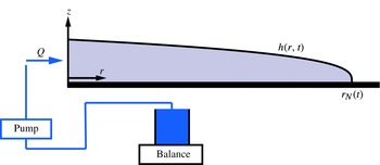
A schematic diagram depicting the experimental set-up in which the response of a spreading, axisymmetric viscous current to a change in flux is measured.

We consider axisymmetric spreading over a horizontal surface of a fluid of density
 $\unicode[STIX]{x1D70C}$
, dynamic viscosity
 $\unicode[STIX]{x1D707}$
and depth
 $h(r,t)$
, which depends on the radial coordinate
 $r$
and time
 $t$
(see figure 1). Once the radial extent of the current is much larger than its depth, the flow is predominantly radial and the pressure within the viscous gravity current is predominantly hydrostatic. The gradients in hydrostatic pressure due to variations in the depth of the current drive a flow resisted by the viscous drag exerted by the bottom boundary. Using lubrication theory, the velocity profile is found to be parabolic, vertical integration provides the local flux and then mass conservation yields the evolution equation (Huppert Reference Huppert1982)
 $$\begin{eqnarray}\frac{\unicode[STIX]{x2202}h}{\unicode[STIX]{x2202}t}=\frac{\unicode[STIX]{x1D70C}g}{3\unicode[STIX]{x1D707}}\frac{1}{r}\frac{\unicode[STIX]{x2202}}{\unicode[STIX]{x2202}r}\left(rh^{3}\frac{\unicode[STIX]{x2202}h}{\unicode[STIX]{x2202}r}\right),\end{eqnarray}$$
where
 $g$
is the gravitational acceleration. At the maximum radial extent of the current,
 $r_{N}(t)$
, the current has zero height and the speed of the translating nose is given by the condition of zero mass flux in the frame of the nose; thus
 $$\begin{eqnarray}h(r_{N})=0\quad \text{and}\quad \frac{\text{d}r_{N}}{\text{d}t}=\left.-\frac{\unicode[STIX]{x1D70C}gh^{2}}{3\unicode[STIX]{x1D707}}\frac{\unicode[STIX]{x2202}h}{\unicode[STIX]{x2202}r}\right|_{r_{N}},\end{eqnarray}$$
respectively.
If the current is initially fed for
 $t>0$
by a constant flux
 $Q$
, then
 $$\begin{eqnarray}\lim _{r\rightarrow 0}\left[-2\unicode[STIX]{x03C0}r\frac{\unicode[STIX]{x1D70C}g}{3\unicode[STIX]{x1D707}}h^{3}\frac{\unicode[STIX]{x2202}h}{\unicode[STIX]{x2202}r}\right]=Q,\end{eqnarray}$$
and it is found that the spreading quickly becomes self-similar and is given by
 $$\begin{eqnarray}h=\left(\frac{3\unicode[STIX]{x1D707}Q}{\unicode[STIX]{x1D70C}g}\right)^{1/4}C^{2/3}H_{\text{s}}(\unicode[STIX]{x1D709}),\quad \text{where}~\unicode[STIX]{x1D709}=\frac{rt^{-1/2}}{C(\unicode[STIX]{x1D70C}gQ^{3}/3\unicode[STIX]{x1D707})^{1/8}},\end{eqnarray}$$
where
 $C$
is a numerical constant (Huppert Reference Huppert1982). The topographic profile of the self-similar current,
 $H_{\text{s}}(\unicode[STIX]{x1D709})$
, satisfies the ordinary differential equation
 $$\begin{eqnarray}-\frac{\unicode[STIX]{x1D709}}{2}\frac{\text{d}H_{\text{s}}}{\text{d}\unicode[STIX]{x1D709}}=\frac{1}{\unicode[STIX]{x1D709}}\frac{\text{d}}{\text{d}\unicode[STIX]{x1D709}}\left(\unicode[STIX]{x1D709}H_{\text{s}}^{3}\frac{\text{d}H_{\text{s}}}{\text{d}\unicode[STIX]{x1D709}}\right)\end{eqnarray}$$
and, if
 $C=0.71502$
, occupies the domain
 $0\leqslant \unicode[STIX]{x1D709}\leqslant 1$
. The radial extent of the current is therefore given by
 $$\begin{eqnarray}r_{N}(t)=C\left(\frac{\unicode[STIX]{x1D70C}gQ^{3}}{3\unicode[STIX]{x1D707}}\right)^{1/8}t^{1/2}.\end{eqnarray}$$
We examine the response of the viscous gravity current to a change from the initial flux
 $Q$
to a new flux
 $\unicode[STIX]{x1D6EC}Q$
at time
 $T$
. This change may be specified as a limiting condition at the origin,
 $$\begin{eqnarray}\lim _{r\rightarrow 0}\left[-2\unicode[STIX]{x03C0}r\frac{\unicode[STIX]{x1D70C}g}{3\unicode[STIX]{x1D707}}h^{3}\frac{\unicode[STIX]{x2202}h}{\unicode[STIX]{x2202}r}\right]=\left\{\begin{array}{@{}ll@{}}Q & 0<t<T,\\ \unicode[STIX]{x1D6EC}Q & t>T,\end{array}\right.\end{eqnarray}$$
or, equivalently, as a global statement of mass conservation,
 $$\begin{eqnarray}2\unicode[STIX]{x03C0}\int _{0}^{r_{N}}hr\,\text{d}r=\left\{\begin{array}{@{}ll@{}}Qt & 0<t<T,\\ QT+\unicode[STIX]{x1D6EC}Q(t-T) & t>T.\end{array}\right.\end{eqnarray}$$
2.2 Scaling the governing equations
The current responds to this change in the flux over a characteristic time scale, relaxing towards a new self-similar solution corresponding to the flux
 $\unicode[STIX]{x1D6EC}Q$
. Simple dimensional analysis might suggest that there is a natural time scale,
 $(\unicode[STIX]{x1D6EC}Q)^{-1/4}(\unicode[STIX]{x1D70C}g/3\unicode[STIX]{x1D707})^{-3/4}$
, given by the new flux
 $\unicode[STIX]{x1D6EC}Q$
and the combination of the physical parameters that characterise the spreading current in (2.1). However, a more careful scaling analysis of the governing equations suggests instead that the behaviour is a function of the initial height and radius of the current at time
 $T$
, and that the transition time
 $T$
provides a new and relevant time scale.
Motivated by the scaling analysis and the similarity solution (2.4), we define vertical and horizontal length scales,
 $$\begin{eqnarray}S_{H}=\left(\frac{3\unicode[STIX]{x1D707}Q}{\unicode[STIX]{x1D70C}g}\right)^{1/4}\quad \text{and}\quad S_{R}=\left(\frac{\unicode[STIX]{x1D70C}gQ^{3}}{3\unicode[STIX]{x1D707}}\right)^{1/8}T^{1/2},\end{eqnarray}$$
written here in terms of the initial flux
 $Q$
, which from (2.4) are scales for the height and radial extent of the initial current at time
 $T$
. Equations (2.1)–(2.3) can now be made non-dimensional by introducing scaled non-dimensional variables
 $\tilde{t}=t/T$
,
 $\tilde{r}=r/S_{R}$
and
 $\tilde{h}=h/S_{H}$
. The response to a change in source conditions is therefore described by the non-dimensional equation
 $$\begin{eqnarray}\frac{\unicode[STIX]{x2202}\tilde{h}}{\unicode[STIX]{x2202}\tilde{t}}=\frac{1}{\tilde{r}}\frac{\unicode[STIX]{x2202}}{\unicode[STIX]{x2202}\tilde{r}}\left(\tilde{r}\tilde{h}^{3}\frac{\unicode[STIX]{x2202}\tilde{h}}{\unicode[STIX]{x2202}\tilde{r}}\right),\end{eqnarray}$$
with boundary conditions
 $$\begin{eqnarray}\tilde{h}(\tilde{r}_{N})=0,\quad \frac{\text{d}\tilde{r}_{N}}{\text{d}\tilde{t}}=\left.-\tilde{h}^{2}\frac{\unicode[STIX]{x2202}\tilde{h}}{\unicode[STIX]{x2202}\tilde{r}}\right|_{\tilde{r}_{N}(\tilde{t})}\end{eqnarray}$$
and
 $$\begin{eqnarray}\lim _{\tilde{r}\rightarrow 0}\left[-2\unicode[STIX]{x03C0}\tilde{r}\tilde{h}^{3}\frac{\unicode[STIX]{x2202}\tilde{h}}{\unicode[STIX]{x2202}\tilde{r}}\right]=\left\{\begin{array}{@{}ll@{}}1 & 0<\tilde{t}<1,\\ \unicode[STIX]{x1D6EC} & \tilde{t}>1.\end{array}\right.\end{eqnarray}$$
In what follows, we drop the tildes for ease of notation.
For
 $t<1$
the current must be independent of any future change in the flux, and the solution is just the similarity solution (2.4), which is
 $h(r,t)=C^{2/3}H_{\text{s}}(\unicode[STIX]{x1D709})$
with
 $\unicode[STIX]{x1D709}=r/Ct^{1/2}$
and extent
 $r_{N}=Ct^{1/2}$
in the scaled variables, where again
 $C=0.71502$
.
At late times,
 $t\gg 1$
, the current must become independent of the initial conditions and return to a self-similar gravity current now of the dimensionless form
 $$\begin{eqnarray}h(r,t)=C^{2/3}\unicode[STIX]{x1D6EC}^{1/4}H_{\text{s}}(\unicode[STIX]{x1D709}/\unicode[STIX]{x1D6EC}^{3/8}),\end{eqnarray}$$
with asymptotic radial extent
 $$\begin{eqnarray}r_{N}(t)\sim r_{\infty }\equiv C\unicode[STIX]{x1D6EC}^{3/8}t^{1/2},\end{eqnarray}$$
reflecting the new flux input at the origin.
The non-dimensional equations governing the relaxation of the current, equations (2.10)–(2.12), contain only the parameter
 $\unicode[STIX]{x1D6EC}$
which is the ratio of fluxes. This indicates that the dimensional time scale
 $\unicode[STIX]{x1D70F}$
over which the current transitions between these two self-similar spreading regimes must be linearly proportional to the time scale
 $T$
with which the equations have been made dimensionless. Hence, we deduce that
 $\unicode[STIX]{x1D70F}$
takes the form
 $$\begin{eqnarray}\unicode[STIX]{x1D70F}=Tf_{p}(\unicode[STIX]{x1D6EC}),\end{eqnarray}$$
where we define
 $f_{p}(\unicode[STIX]{x1D6EC})$
to be the time measured from
 $t=0$
for the radial extent of the current to relax to within a fraction
 $p$
of the final, self-similar solution given by (2.13), i.e. such that
 $|r_{N}-r_{\infty }|<pr_{\infty }$
. In particular,
 $$\begin{eqnarray}f_{p}(1)=1,\quad f_{p}(\unicode[STIX]{x1D6EC})\geqslant 1\quad \text{for }\unicode[STIX]{x1D6EC}\neq 1.\end{eqnarray}$$
The proportionality to
 $T$
, and the functional form of
 $f_{p}(\unicode[STIX]{x1D6EC})$
, derived analytically in § 3, may be anticipated by the following physical argument. The spreading rate of a viscous gravity current depends on the volume of fluid within the current. For currents in which the flux changes by a factor
 $\unicode[STIX]{x1D6EC}$
at time
 $T$
there is a volumetric deficit (or excess)
 $\unicode[STIX]{x0394}V$
from times less than
 $T$
, which may be expressed in terms of an equivalent shift
 $\unicode[STIX]{x0394}T$
in the time origin of the final self-similar state:
 $\unicode[STIX]{x0394}V=(\unicode[STIX]{x1D6EC}Q-Q)T=\unicode[STIX]{x1D6EC}Q\,\unicode[STIX]{x0394}T$
. Hence, we may expect a time scale
 $$\begin{eqnarray}\unicode[STIX]{x1D70F}\sim \unicode[STIX]{x0394}T=|1-1/\unicode[STIX]{x1D6EC}|T.\end{eqnarray}$$
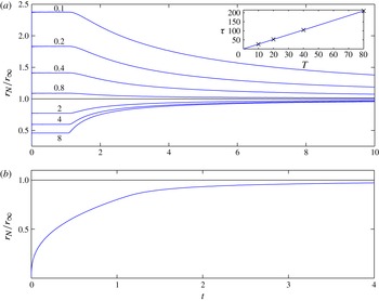
(a) The response of the current, as characterised by the radial extent
 $r_{N}/r_{\infty }$
, to a change in the flux for
 $\unicode[STIX]{x1D6EC}=0.1$
, 0.2, 0.4, 0.8, 2, 4 and 8, where
 $r_{\infty }$
is the asymptotic radial spreading rate. Inset shows the relaxation time
 $\unicode[STIX]{x1D70F}$
as a function of
 $T$
, where relaxation times are measured for
 $r_{N}/r_{\infty }=0.9$
with
 $\unicode[STIX]{x1D6EC}=2$
and where the crosses,
 $\times$
, denote the numerical results. (b) The response of the current for the singular case
 $\unicode[STIX]{x1D6EC}=0$
where
 $r_{\infty }$
is the radius of a current propagating with constant volume (and zero flux).

2.3 Numerical results
To investigate the detailed form of
 $f_{p}(\unicode[STIX]{x1D6EC})$
we determined numerical solutions to (2.10) with boundary conditions (2.11)–(2.12). The form of the relaxation towards self-similarity may be readily assessed by plotting
 $r_{N}(t)/r_{\infty }(t)$
against
 $t$
for a variety of
 $\unicode[STIX]{x1D6EC}$
, as shown in figure 2(a). For
 $t<1$
,
 $r_{N}/r_{\infty }$
is a constant, equal to
 $\unicode[STIX]{x1D6EC}^{-3/8}$
, confirming the initial self-similarity (2.4). Then for
 $t>1$
,
 $r_{N}/r_{\infty }$
increases up to
 $1$
for
 $\unicode[STIX]{x1D6EC}>1$
and decreases down to
 $1$
for
 $0<\unicode[STIX]{x1D6EC}<1$
, showing that the current asymptotically adjusts to a new self-similar solution that propagates with the rate determined by the new input flux
 $\unicode[STIX]{x1D6EC}Q$
.
A singular and important limiting case is the relaxation from a constant flux to a fixed-volume current (
 $\unicode[STIX]{x1D6EC}=0$
). For late times,
 $t\gg 1$
, the radial extent of the constant-volume, axisymmetric viscous current spreading with constant volume again becomes independent of the initial conditions and returns to a self-similar gravity current, now of the form
 $$\begin{eqnarray}r_{\infty }=C_{V}t^{1/8},\end{eqnarray}$$
which may be written in dimensional form as
 $$\begin{eqnarray}r_{\infty }=C_{V}\left(\frac{\unicode[STIX]{x1D70C}gV^{3}}{3\unicode[STIX]{x1D707}}\right)^{1/8}t^{1/8},\end{eqnarray}$$
where
 $C_{V}=0.894$
(Huppert Reference Huppert1982) and
 $V=QT$
is the volume of fluid injected into the current in the period
 $0\leqslant t\leqslant T$
. The comparison between the numerically calculated radial extent and the constant-volume similarity solution is shown in figure 2(b).
The results of figure 2(a,b) may be summarised by plotting
 $f_{p}(\unicode[STIX]{x1D6EC})$
for
 $p=0.15$
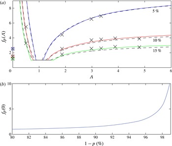
, 0.1 and 0.05 as shown in figure 3. Here we see that
 $f_{p}(\unicode[STIX]{x1D6EC})$
is an increasing function of
 $\unicode[STIX]{x1D6EC}>1$
, and approaches a constant value for
 $\unicode[STIX]{x1D6EC}\gg 1$
because for large
 $\unicode[STIX]{x1D6EC}$
the propagation rate of the new (relatively high flux) current is independent of the initial response (to a much smaller flux). The function
 $f_{p}(\unicode[STIX]{x1D6EC})$
increases with decreasing
 $\unicode[STIX]{x1D6EC}<1$
, and approaches infinity as
 $\unicode[STIX]{x1D6EC}\rightarrow 0$
, reflecting the fact that it takes an ever increasing time for the similarity solution describing the new current (relatively very small flux) to reach the extent of the initial current.
(a) Graph of the dimensionless transition time
 $f_{p}(\unicode[STIX]{x1D6EC})$
for a range of values of the flux ratio
 $\unicode[STIX]{x1D6EC}$
as determined numerically (solid lines, colour online), where
 $f_{p}$
is defined by the criterion that the numerical solutions,
 $r_{N}(t)$
, are within a fraction
 $p$
(15 %, 10 % or 5 %) of the similarity solution
 $r_{\infty }(t)$
for a current propagating with a constant flux. The theoretical estimates (3.11) of
 $f_{p}(\unicode[STIX]{x1D6EC})$
are shown by black dashed lines. Experimental values for
 $f_{p}(\unicode[STIX]{x1D6EC})$
are shown as crosses,
 $\times$
. (b) Graph of
 $f_{p}(0)$
for the singular case
 $\unicode[STIX]{x1D6EC}=0$
showing when the radial extent of a current transitioning from constant flux to constant volume is within a fraction
 $p$
of the asymptotic value,
 $r_{N}/r_{\infty }>1-p$
.

The case of
 $\unicode[STIX]{x1D6EC}=0$
is treated differently to
 $\unicode[STIX]{x1D6EC}>0$
since the numerical solutions,
 $r_{N}$
, must be compared with the theoretically determined
 $r_{\infty }$
for a constant volume (zero flux) release with initial volume
 $V=QT$
as described by (2.18). The point
 $f_{p}(0)$
is both singular and finite. The distance reached by the current of a flux
 $Q$
after a propagation time
 $T$
is already within 20 % of the theoretical radius
 $r_{\infty }$
and decreases less rapidly than the constant-volume release since
 $t^{1/8}\ll t^{1/2}$
. As a result, the current catches up very quickly, in comparison to the case
 $0<\unicode[STIX]{x1D6EC}\ll 1$
, where both currents are propagating at the same rate,
 $t^{1/2}$
, as can be seen in figure 3(b).
3 Asymptotic approach to self-similarity
As illustrated in figure 2, a gravity current described by the non-dimensional equations (2.10)–(2.12) relaxes towards the similarity solution (2.13)–(2.14) following the change in the source flux at non-dimensional time
 $t=1$
. We analyse the asymptotic rate of approach to self-similarity as follows.
Motivated by the form of (2.13)–(2.14), we change variables by defining
 $$\begin{eqnarray}h(r,t)=C^{2/3}\unicode[STIX]{x1D6EC}^{1/4}H(\unicode[STIX]{x1D702},s),\quad r_{N}(t)=C\unicode[STIX]{x1D6EC}^{3/8}t^{1/2}Y_{N}(s),\end{eqnarray}$$
where
 $\unicode[STIX]{x1D702}=\unicode[STIX]{x1D709}/\unicode[STIX]{x1D6EC}^{3/8}$
and
 $s=\ln t$
. Expressed in the new variables, equations (2.10)–(2.12) become
 $$\begin{eqnarray}\displaystyle & \displaystyle \frac{\unicode[STIX]{x2202}H}{\unicode[STIX]{x2202}s}-\frac{\unicode[STIX]{x1D702}}{2}\frac{\unicode[STIX]{x2202}H}{\unicode[STIX]{x2202}\unicode[STIX]{x1D702}}=\frac{1}{\unicode[STIX]{x1D702}}\frac{\unicode[STIX]{x2202}}{\unicode[STIX]{x2202}\unicode[STIX]{x1D702}}\left(\unicode[STIX]{x1D702}H^{3}\frac{\unicode[STIX]{x2202}H}{\unicode[STIX]{x2202}\unicode[STIX]{x1D702}}\right), & \displaystyle\end{eqnarray}$$
 $$\begin{eqnarray}\displaystyle & \displaystyle H(Y_{N})=0,\quad \frac{\text{d}Y_{N}}{\text{d}s}+\frac{Y_{N}}{2}=\left.-H^{2}\frac{\unicode[STIX]{x2202}H}{\unicode[STIX]{x2202}\unicode[STIX]{x1D702}}\right|_{Y_{N}} & \displaystyle\end{eqnarray}$$
and
 $$\begin{eqnarray}\lim _{\unicode[STIX]{x1D702}\rightarrow 0}-\unicode[STIX]{x1D702}H^{3}\frac{\unicode[STIX]{x2202}H}{\unicode[STIX]{x2202}\unicode[STIX]{x1D702}}=\frac{C^{-8/3}}{2\unicode[STIX]{x03C0}}\quad \text{for}~s>0.\end{eqnarray}$$
(A different source flux condition applies for
 $s<0$
, i.e.
 $t<1$
, but is not relevant here.)
The late-time similarity solution (2.13)–(2.14) now corresponds to a steady solution
 $H(\unicode[STIX]{x1D702},s)=H_{\text{s}}(\unicode[STIX]{x1D702})$
,
 $Y_{N}(s)=1$
of (3.2)–(3.4), and the use of
 $s=\ln t$
as the time-like variable keeps the equations autonomous. It is thus possible to determine the stability of the similarity solution by the usual process of linearisation about this steady solution and looking for perturbation eigenmodes proportional to
 $\text{e}^{\unicode[STIX]{x1D70E}s}(=t^{\unicode[STIX]{x1D70E}})$
.
Let
 $Y_{N}=1+\unicode[STIX]{x1D716}Y_{1}\text{e}^{\unicode[STIX]{x1D70E}s}+O(\unicode[STIX]{x1D716}^{2})$
and
 $H(\unicode[STIX]{x1D702},s)=H_{\text{s}}(\unicode[STIX]{x1D702})+\unicode[STIX]{x1D716}H_{1}(\unicode[STIX]{x1D702})\text{e}^{\unicode[STIX]{x1D70E}s}+O(\unicode[STIX]{x1D716}^{2})$
. The condition
 $H(Y_{N})=0$
linearises for
 $\unicode[STIX]{x1D716}\ll 1$
to
 $Y_{1}H_{\text{s}}^{\prime }+H_{1}\rightarrow 0$
as
 $\unicode[STIX]{x1D702}\rightarrow 1$
, where it is known from the steady solution that
 $H_{\text{s}}^{3}\sim 3(1-\unicode[STIX]{x1D702})/2$
as
 $\unicode[STIX]{x1D702}\rightarrow 1$
. Linearizing the other equations similarly, we find after some algebra that the perturbation eigenmode problem can be written as
 $$\begin{eqnarray}\unicode[STIX]{x1D70E}H_{1}-\frac{\unicode[STIX]{x1D702}}{2}H_{1}^{\prime }=\unicode[STIX]{x1D702}^{-1}[\unicode[STIX]{x1D702}(H_{\text{s}}^{3}H_{1})^{\prime }]^{\prime },\end{eqnarray}$$
 $$\begin{eqnarray}H_{\text{s}}^{2}H_{1}\rightarrow {\textstyle \frac{1}{2}}Y_{1}\quad \text{and}\quad -(H_{\text{s}}^{2}H_{1})^{\prime }\rightarrow \left(\unicode[STIX]{x1D70E}+{\textstyle \frac{1}{2}}\right)Y_{1}\quad \text{as}~\unicode[STIX]{x1D702}\rightarrow 1,\end{eqnarray}$$
 $$\begin{eqnarray}\lim _{\unicode[STIX]{x1D702}\rightarrow 0}\unicode[STIX]{x1D702}(H_{\text{s}}^{3}H_{1})^{\prime }=0.\end{eqnarray}$$
The boundary conditions (3.6) at the nose are written as limits because
 $\unicode[STIX]{x1D702}=1$
is a singular point of the differential equation (3.5), where
 $H_{\text{s}}\propto (1-\unicode[STIX]{x1D702})^{1/3}$
and
 $H_{1}\propto (1-\unicode[STIX]{x1D702})^{-2/3}$
. Physically, this just corresponds to the generic behaviour of
 $h(r,t)$
near a propagating fluid front in lubrication theory.
One can show directly from (3.5)–(3.7) that
 $(\unicode[STIX]{x1D70E}+1)\int _{0}^{1}H_{1}\unicode[STIX]{x1D702}\,\text{d}\unicode[STIX]{x1D702}=0$
. Physically, this shows that all of the eigenvalues and eigenmodes, except for
 $\unicode[STIX]{x1D70E}=-1$
, correspond to zero perturbation to the volume of the gravity current, and to radial redistribution of the fluid in the current towards its self-similar shape.
The exception is the eigenvalue
 $\unicode[STIX]{x1D70E}=-1$
, for which the eigenmode is
 $H_{1}=-\unicode[STIX]{x1D702}H_{\text{s}}^{\prime }/2$
,
 $Y_{1}=1/2$
, as can be verified directly from (3.5)–(3.7). Physically, this eigenmode can be interpreted in two illuminating ways. First, the eigenmode corresponds to making a small displacement
 $t\rightarrow t+\unicode[STIX]{x1D716}$
in the time origin of the similarity solution (2.13)–(2.14), which gives a new solution due to the time-translational invariance of the evolution equation (2.10). Alternatively, it can be shown directly from (3.2)–(3.4) that
 $$\begin{eqnarray}2\unicode[STIX]{x03C0}\int _{0}^{1}\left(-{\textstyle \frac{1}{2}}\unicode[STIX]{x1D702}H_{\text{s}}^{\prime }\right)\unicode[STIX]{x1D702}\,\text{d}\unicode[STIX]{x1D702}=[2\unicode[STIX]{x03C0}\unicode[STIX]{x1D702}H_{\text{s}}^{3}H_{\text{s}}^{\prime }]_{0}^{1}=C^{-8/3}\end{eqnarray}$$
and then, with
 $H=H_{\text{s}}+\unicode[STIX]{x1D716}H_{1}t^{-1}$
, from (3.1) that
 $$\begin{eqnarray}2\unicode[STIX]{x03C0}\int _{0}^{r_{N}}hr\,\text{d}r=\unicode[STIX]{x1D6EC}t+\unicode[STIX]{x1D716}\unicode[STIX]{x1D6EC}.\end{eqnarray}$$
Hence the eigenmode also corresponds to the late-time behaviour of a current with an excess (non-dimensional) volume
 $\unicode[STIX]{x1D716}\unicode[STIX]{x1D6EC}$
.
The significance of the second interpretation is that it does not matter whether the excess volume was supplied at early times by a uniform flux
 $\unicode[STIX]{x1D6EC}$
over an extra time interval
 $(-\unicode[STIX]{x1D716},0)$
(i.e. a shifted time origin), or by an extra flux
 $\unicode[STIX]{x1D716}\unicode[STIX]{x1D6EC}$
over the early time interval
 $(0,1)$
(i.e. a different initial flux): because of mass conservation, the amplitude of the late-time eigenmode with
 $\unicode[STIX]{x1D70E}=-1$
is simply obtained from the magnitude of any early non-zero perturbation to the volume of the current.
This analysis provides mathematical justification for the physical statement, expressed in § 2.2, that the dimensional excess volume
 $(Q-\unicode[STIX]{x1D6EC}Q)T$
at time
 $T$
becomes asymptotically equivalent at long times to a shift in time origin. In non-dimensional terms, the excess volume gives
 $\unicode[STIX]{x1D716}\unicode[STIX]{x1D6EC}=1-\unicode[STIX]{x1D6EC}$
and thus
 $$\begin{eqnarray}Y_{N}(t)\sim 1+\frac{(1/\unicode[STIX]{x1D6EC})-1}{2t}\quad \text{as}~t\rightarrow \infty .\end{eqnarray}$$
Recalling the definition of
 $f_{p}$
in (2.15) as the time for the radial extent of the current to relax to within a fraction
 $p$
of the self-similar value, we can now use (3.10) to estimate
 $$\begin{eqnarray}f_{p}\sim \frac{|(1/\unicode[STIX]{x1D6EC})-1|}{2p}\end{eqnarray}$$
for sufficiently small values of
 $p$
that the relaxation time is dominated by the late-time linear regime. In fact, as shown in figure 2, equation (3.11) provides a remarkably good approximation even for quite short relaxation times.
The form of (3.11) confirms that the transition from a constant flux to constant volume,
 $\unicode[STIX]{x1D6EC}\rightarrow 0$
, is a singular limit. For the case
 $\unicode[STIX]{x1D6EC}=0$
, the current has a fixed volume after the input flux is stopped at dimensional time
 $T$
. The linear stability of the fixed-volume similarity solution was analysed by Grundy & McLaughlin (Reference Grundy and McLaughlin1982). The most slowly decaying eigenmode again has eigenvalue
 $\unicode[STIX]{x1D70E}=-1$
and again corresponds to making a small displacement in the time origin of the similarity solution. However, it is no longer possible to calculate the magnitude of this time displacement by equating it to an excess volume divided by the new flux, because the new flux is zero. The
 $t^{-1}$
decay shows that
 $f_{p}(0)\sim A/p$
as
 $p\rightarrow 0$
for some constant
 $A$
. A fit to the data in figure 3(b) suggests
 $A\approx 0.10$
.
4 Experiments
To verify the theoretically determined form of the equilibration time
 $\unicode[STIX]{x1D70F}$
, we conducted a series of experiments in which a constant flux
 $Q$
of blue-dyed glycerine was input through a hole in the centre of a horizontal glass sheet, of size 1 m
 $\times$
1 m, using a Watson-Marlow peristaltic pump (see figure 1). The fluid was allowed to spread axisymmetrically and at time
 $T$
the incoming flux was changed from
 $Q$
to
 $\unicode[STIX]{x1D6EC}Q$
. The mass flux from the feeder reservoir was, at all times, independently recorded on an electronic balance. A series of images, taken every 10 seconds with a digital camera, recorded the radial flow of glycerine across the glass sheet from which we determined the extent as a function of time.
A first set of experiments were conducted with a constant flux
 $Q$
to check the agreement with the theoretically determined
 $r_{N}$
, given by (2.6). We found that the experiments were in good agreement with the power law for
 $r_{N}$
, and that the experimentally determined pre-factor,
 $C_{exp}=0.964C$
, was within 5 % of the theoretically predicted value. As a result, when analysing the results for the experiments in which we change the flux from
 $Q$
to
 $\unicode[STIX]{x1D6EC}Q$
at time
 $T$
, we find the equilibration time
 $\unicode[STIX]{x1D70F}$
by evaluating when the experimental results for a given
 $\unicode[STIX]{x1D6EC}$
reach within a fraction
 $p$
of the theoretically determined
 $r_{N}$
multiplied by the factor
 $0.964$
. The values of
 $f_{p}(\unicode[STIX]{x1D6EC})$
for these experiments are shown as crosses,
 $\times$
, in figure 3(a) and are in good agreement with the numerical and asymptotic solutions.
For the case of
 $\unicode[STIX]{x1D6EC}=0$
, we compared the experimental values,
 $r_{exp}$
, with the numerical solutions,
 $r_{N}$
, for a change in flux from
 $Q$
to constant volume
 $V=QT$
. We matched the experimental results with the numerical solutions at the end point of each run by multiplying
 $r_{exp}$
by the factor
 $r_{N}(t_{end})/r_{exp}(t_{end})=1.079$
. We found that the curves for the
 $r_{exp}$
and
 $r_{N}$
lay perfectly on top of each other, implying that the
 $r_{exp}(t)$
and
 $r_{N}(t)$
differed by a multiplicative factor, as in the case
 $\unicode[STIX]{x1D6EC}>0$
. By taking this into account, the values for
 $f_{p}(\unicode[STIX]{x1D6EC})$
for the experimental results are in very good agreement with the numerical solutions, as can be seen in figure 3(a).
5 Generalising the results
The results presented for the case of an axisymmetric, viscous gravity current apply more generally to linearly spreading viscous currents, and to axisymmetric and linearly spreading gravity currents within a porous medium. These currents share the common property that they are buoyancy driven, and hence their velocity is proportional to horizontal gradients in the internal hydrostatic pressure and hence depth of the fluid layer. Perhaps more importantly, these currents are long and thin, so obey an evolution equation of the form
 $$\begin{eqnarray}\frac{\unicode[STIX]{x2202}h}{\unicode[STIX]{x2202}t}=\unicode[STIX]{x1D6FD}\unicode[STIX]{x1D735}\boldsymbol{\cdot }(h^{n}\unicode[STIX]{x1D735}h),\end{eqnarray}$$
where
 $\unicode[STIX]{x1D735}$
is now the horizontal gradient operator, and where
 $$\begin{eqnarray}\unicode[STIX]{x1D6FD}=\unicode[STIX]{x1D70C}g/3\unicode[STIX]{x1D707}\quad \text{with}~n=3\end{eqnarray}$$
for a viscous current spreading with a free surface over a horizontal base (Huppert Reference Huppert1982), and
 $$\begin{eqnarray}\unicode[STIX]{x1D6FD}=\unicode[STIX]{x0394}\unicode[STIX]{x1D70C}gk/\unicode[STIX]{x1D719}\unicode[STIX]{x1D707}\quad \text{with}~n=1\end{eqnarray}$$
for a current spreading in a porous medium of permeability
 $k$
, porosity
 $\unicode[STIX]{x1D719}$
, and with density difference
 $\unicode[STIX]{x0394}\unicode[STIX]{x1D70C}$
with respect to the ambient (Huppert & Woods Reference Huppert and Woods1995). The evolution equation is subject to the boundary conditions
 $$\begin{eqnarray}h=0\quad \text{and}\quad -\unicode[STIX]{x1D6FD}h^{n}\unicode[STIX]{x1D735}h=\mathbf{0}\end{eqnarray}$$
at the front of the current, which is at
 $x=x_{N}$
for a linearly spreading current with the depth of the fluid given by
 $h=h(x,t)$
, and at
 $r=r_{N}$
for an axisymmetric current with fluid depth
 $h=h(r,t)$
. At the origin, we impose a constraint on the flux:
 $$\begin{eqnarray}\left.\begin{array}{@{}ll@{}}\text{linear} & \lim _{x\rightarrow 0}-\unicode[STIX]{x1D6FD}h^{n}\displaystyle \frac{\unicode[STIX]{x2202}h}{\unicode[STIX]{x2202}x}\\ \text{axisymmetric} & \lim _{r\rightarrow 0}-2\unicode[STIX]{x03C0}r\unicode[STIX]{x1D6FD}h^{n}\displaystyle \frac{\unicode[STIX]{x2202}h}{\unicode[STIX]{x2202}r}\end{array}\right\}=\left\{\begin{array}{@{}ll@{}}Q & 0<t<T,\\ \unicode[STIX]{x1D6EC}Q & t>T.\end{array}\right.\end{eqnarray}$$
In each case we find that, as before, for a change in the source conditions at time
 $T$
the currents are most naturally scaled by the height and extent of the current at that time rather than any time scale constructed from the dimensional quantities in the system. The fixed-flux similarity solutions to (5.1) that apply for
 $t<T$
satisfy the scalings
 $$\begin{eqnarray}h\sim (Q^{2}/\unicode[STIX]{x1D6FD})^{1/(n+2)}t^{1/(n+2)}\quad \text{and}\quad x_{N}\sim (Q^{n}\unicode[STIX]{x1D6FD})^{1/(n+2)}t^{(n+1)/(n+2)},\end{eqnarray}$$
 $$\begin{eqnarray}h\sim (Q/\unicode[STIX]{x1D6FD})^{1/(n+1)}\quad \text{and}\quad r_{N}\sim (Q^{n}\unicode[STIX]{x1D6FD})^{1/2(n+1)}t^{1/2},\end{eqnarray}$$
for linear spreading and axisymmetric spreading, respectively. If we define vertical and horizontal scales
 $S_{H}$
,
 $S_{X}$
and
 $S_{R}$
by evaluating these scales at
 $t=T$
, and use these and the time
 $T$
to non-dimensionalise the full problem, then we find again that the dimensionless problem depends only on the flux ratio
 $\unicode[STIX]{x1D6EC}$
(and the exponent
 $n$
). We deduce again that, in each case, the dimensional time scale for adjustment is linearly proportional to
 $T$
and takes the form
 $$\begin{eqnarray}\unicode[STIX]{x1D70F}=Tf_{p}(\unicode[STIX]{x1D6EC},n),\end{eqnarray}$$
where
 $p$
is the fractional deviation from the ultimate spreading behaviour.
In each case, once the flux is altered the current approaches a new self-similar spreading behaviour characterised by the final flux
 $\unicode[STIX]{x1D6EC}Q$
. For
 $\unicode[STIX]{x1D6EC}\neq 0$
the time scale over which the current adjusts to the new self-similar state may again be estimated by a shift in the time origin equivalent to the mass excess (or deficit) due to the initial injection at flux
 $Q$
. By following the line of argument given for an axisymmetric, viscous gravity current in § 3, we deduce that
 $$\begin{eqnarray}f_{p}\approx \unicode[STIX]{x1D6FE}|1/\unicode[STIX]{x1D6EC}-1|/p,\end{eqnarray}$$
where
 $\unicode[STIX]{x1D6FE}$
is the exponent of the self-similar horizontal spread proportional to
 $t^{\unicode[STIX]{x1D6FE}}$
, i.e.
 $\unicode[STIX]{x1D6FE}=(n+1)/(n+2)$
for linear spreading and
 $\unicode[STIX]{x1D6FE}=1/2$
(independent of
 $n$
) for axisymmetric spreading (see (5.6)–(5.7)). The case
 $\unicode[STIX]{x1D6EC}=0$
is again a singular limit.
In an alternative scenario, we could consider a fixed-volume current of volume
 $V$
that is allowed to spread for time
 $T$
before injection at the origin commences with a source flux
 $Q$
. By again scaling the equations with the height and extent of the current at the transition time
 $T$
, it becomes clear that the relaxation time must be of the form
 $\unicode[STIX]{x1D70F}=Tf_{V}(QT/V,n)$
for some function
 $f_{V}$
, so
 $\unicode[STIX]{x1D70F}$
is again proportional to
 $T$
.
6 Conclusion
The spreading of viscous gravity currents, and of gravity currents within porous media, is ubiquitous within the natural environment and a host of industrial settings. The theoretical underpinnings of models describing the buoyancy-driven flow have, to date, focused primarily on settings in which the conditions on the flow are held fixed; currents are often either fed by a constant flux or spread as a constant volume. In each case a characteristic, self-similar spreading behaviour may be found and compared with the results of laboratory, industrial or environmental observations. A large-scale, and timely, example is the spreading of buoyant CO
 $_{2}$
in the Sleipner field underneath the North Sea (Boait et al.
Reference Boait, White, Bickle, Chadwick, Neufeld and Huppert2012). Previous work has shown that the seismic images of the spreading CO
 $_{2}$
plume may be successfully interpreted using the theory of axisymmetric gravity currents spreading in a porous medium (Bickle et al.
Reference Bickle, Chadwick, Huppert, Hallworth and Lyle2007). More recent processing of the seismic images of the spreading CO
 $_{2}$
plume also demonstrate that the flow is, to good approximation, unconfined and hence independent of depth of the aquifer (Cowton et al.
Reference Cowton, Neufeld, White, Bickle, White and Chadwick2016). However, for projects in which injected CO
 $_{2}$
spans the depth of the aquifer the motion of ambient fluid (e.g. water) may no longer be neglected. The transition from two-dimensional, confined currents fed by a constant flux to those with constant volume has been analysed previously by Hesse et al. (Reference Hesse, Tchelepi, Cantwell and Orr2007) who showed that for confined aquifers the transition time may also depend on the ratio of fluid viscosities.
This work provides a physical and theoretical argument, along with experimental verification, of the time scales over which diffusive, spreading gravity currents adjust to changes in their source conditions. In the case of CO
 $_{2}$
spreading in Sleipner under the North Sea, these calculations may be used to predict the evolution of the spreading behaviour from the current injection phase, to the constant-volume post-injection phase of monitoring. The same arguments can be used in a host of settings and might usefully be applied to the time scale for glacial flows (essentially viscous gravity currents) to accommodate changes in climatic precipitation patters.
Acknowledgements
We are grateful for generous financial support from the Bridgewater summer-project scheme (T.V.B.), from a Leverhulme Fellowship (H.E.H.) and from a Royal Society University Research Fellowship (J.A.N.).
Appendix A
We show here that the results of the equilibration
 $\unicode[STIX]{x1D70F}$
in response to a flux change from
 $Q$
to
 $\unicode[STIX]{x1D6EC}Q$
being linearly proportional to the injection period
 $T$
(and independent of all other parameters) is also true for high-Reynolds-number currents. Consider the one-dimensional shallow water model of flow beneath a free surface with height
 $h(x,t)$
where
 $x$
is the extent of the current. The governing equations are given by
 $$\begin{eqnarray}\displaystyle & \displaystyle \frac{\unicode[STIX]{x2202}h}{\unicode[STIX]{x2202}t}+\frac{\unicode[STIX]{x2202}}{\unicode[STIX]{x2202}x}(uh)=0, & \displaystyle\end{eqnarray}$$
 $$\begin{eqnarray}\displaystyle & \displaystyle \frac{\unicode[STIX]{x2202}}{\unicode[STIX]{x2202}t}(uh)+\frac{\unicode[STIX]{x2202}}{\unicode[STIX]{x2202}x}\left(u^{2}h+\frac{1}{2}gh^{2}\right), & \displaystyle\end{eqnarray}$$
with boundary condition on the flux at
 $x=0$
of
 $$\begin{eqnarray}uh=\left\{\begin{array}{@{}ll@{}}Q & 0<t<T,\\ \unicode[STIX]{x1D6EC}Q & t>T.\end{array}\right.\end{eqnarray}$$
A suitable transformation of variables is given by
 $$\begin{eqnarray}h=(Q^{2}/g)^{1/3}H,\quad u=(gQ)^{1/3}U\quad \text{and}\quad x=(gQ)^{1/3}X.\end{eqnarray}$$
The governing equations then become
 $$\begin{eqnarray}\displaystyle & \displaystyle \frac{\unicode[STIX]{x2202}H}{\unicode[STIX]{x2202}t}+\frac{\unicode[STIX]{x2202}}{\unicode[STIX]{x2202}X}(UH)=0, & \displaystyle\end{eqnarray}$$
 $$\begin{eqnarray}\displaystyle & \displaystyle \frac{\unicode[STIX]{x2202}}{\unicode[STIX]{x2202}t}\left(UH\right)+\frac{\unicode[STIX]{x2202}}{\unicode[STIX]{x2202}X}\left(U^{2}H+\frac{1}{2}H^{2}\right), & \displaystyle\end{eqnarray}$$
with boundary condition on the flux at
 $X=0$
of
 $$\begin{eqnarray}UH=\left\{\begin{array}{@{}ll@{}}1 & 0<t<T,\\ \unicode[STIX]{x1D6EC} & t>T.\end{array}\right.\end{eqnarray}$$
The only physical parameter remaining in the system is
 $T$
, with dimensions of time, and
 $\unicode[STIX]{x1D6EC}$
, which is non-dimensional. Hence the equilibration time
 $\unicode[STIX]{x1D70F}$
must be linearly proportional to
 $T$
and of the form
 $$\begin{eqnarray}\unicode[STIX]{x1D70F}=Tf(\unicode[STIX]{x1D6EC}),\end{eqnarray}$$
where
 $\unicode[STIX]{x1D70F}$
is measured from
 $t=0$
.