1. Introduction
With the enormous global concerns about climate change and biodiversity in recent years (Jenkins et al., Reference Jenkins, Ephraums and Houghton1990; Magurran, Reference Magurran2004), grassland has received more attention than ever before as a type of natural resource that plays an important role in sequestrating carbon (Conant et al., Reference Conant, Paustian and Elliott2001) and preserving biodiversity (Tilman and Downing, Reference Tilman and Downing1994). Inside China, concerns over the severe environmental consequences of grassland degradation, such as sandstorms and desertification, have stimulated a large literature on understanding the factors leading to degradation. These factors include overgrazing, population pressure, urbanization, conversion to crop land and climatic factors (Smil, Reference Smil1993; Gong et al., Reference Gong, Harazono, Oikawa, Zhao, He and Chang2000; Zhang et al., Reference Zhang, Liu, Bai, Shen, Yan, Ding, Li and Zheng2006; Akiyama and Kawamura, Reference Akiyama and Kawamura2007; Liu et al., Reference Liu, Michalk, Bai, Yu and Chen2008).
At the same time, in the rapidly growing literature on deforestation, roads are identified as one of the important determinants. In many instances roads are found to exacerbate the rate of deforestation (e.g., Chomitz and Gray, Reference Chomitz and Gray1996; Mertens and Lambin, Reference Mertens and Lambin1997; Pfaff, Reference Pfaff1999; Cropper et al., Reference Cropper, Puri and Griffiths2001). When new roads are constructed or when existing roads are widened or paved, the access to forested area is less costly. Furthermore, by lowering transport costs, roads also increase the value of agricultural products, accelerating the clearing of forested areas for agriculture. However, in a few studies, the opposite impacts are identified. Andersen et al. (Reference Andersen, Granger, Reis, Weinhold and Wunder2002) find that new roads reduce the rate of deforestation in the Brazilian Amazon, at least in counties with substantial prior clearing of forest. The suggested causal mechanism is that roads provide a focal point for local development, drawing pressure away from the forested hinterland. Similarly, Deininger and Minten (Reference Deininger and Minten2002) find that roads weaken the negative impact on forests of high poverty levels in Southern Mexico.
In the grassland literature, only a small group of studies have focused on the relationship between roads and grassland degradation. Mostly the ecological effects of roads on the grassland ecosystem are considered (White et al., Reference White, Murray and Rohweder2000; Wu and Ci, Reference Wu and Ci2002). For example, the construction of roads separates formerly integrated ecosystems into separate and ecologically more vulnerable parts. Road traffic significantly reduces the regular breeding activities of several species of grassland birds (Forman et al., Reference Forman, Reineking and Hersperger2002). Roads have also been shown to increase the possibility of the invasion of non-native species (Forman, Reference Forman2000).
A smaller number of studies focus on the non-ecological impacts of roads on the grassland. For example, in the suburbs of Melbourne, the probability of a patch of grassland being destroyed increases for patches closer to a major road, since the completion of the road triggers economic development in suburban areas (Williams et al., Reference Williams, Morgan, McDonnell and McCarthy2005). In a case study from Colombia it was found that, because of increased stocking rates near roads, pasture was so damaged by trampling that it was not able to take advantage of the relatively high levels of fertility of the soil (Conant et al., Reference Conant, Paustian and Elliott2001). Inside China, Gao et al. (Reference Gao, Wan, Li, Sheng, Jiangcun, Wang and Li2007) show that human activity in the region near to the roads of North Tibet had a negative effect on the grasslands. The common finding in these papers is that roads led to grassland degradation. The logic of these authors is that, when there are roads in a specific area (or when a road is widened or improved), pressure will rise on the grassland resources as it becomes easier to access and/or more profitable to exploit the value that is associated with the grassland resource. Hence, it is predicted that roads will make the grassland cover fall.
On the other hand, some authors find that roads do not necessarily lead to grassland destruction (Zhang et al., Reference Zhang, Yan, Liu, Bai, Li and Zheng2002; Williams et al., Reference Williams, Morgan, McCarthy and McDonnell2006). Instead the impact of roads on grasslands depends on the type of road and the type of grassland. In a case study from the source region of China's Yellow River, Zhang et al. (Reference Zhang, Liu, Bai, Shen, Yan, Ding, Li and Zheng2006) find roads not to have a negative impact on grassland. Gao et al. (Reference Gao, Wan, Li, Sheng, Jiangcun, Wang and Li2007) also find that, although grasslands have shown clear signs of degradation in some of the high elevation regions of Northern Tibet, in other areas (especially in those areas in which human activity is relatively intense), roads have actually led to higher quality grassland resources. These authors postulate that better road access allows for more successful implementation of grassland restoration projects. The implicit logic of these papers is that, when a road enters an area, it allows agents access to new resources from outside the grassland which may actually reduce pressure on (or increase investment for restoration in) the local economy's grassland resource base.
A consensus is yet to form, however, because in addition to the paucity of studies on grasslands and roads, inadequate data and methodological shortcomings weaken some findings in this literature. For example, many studies (e.g., Zhang et al., Reference Zhang, Yan, Liu, Bai, Li and Zheng2002; Gao et al., Reference Gao, Wan, Li, Sheng, Jiangcun, Wang and Li2007) only look at the relationship between roads and the grasslands without controlling for other covariates, while others (for example, Liu et al., Reference Liu, Michalk, Bai, Yu and Chen2008), include only a single control variable. Moreover, only one paper to our knowledge – Williams (Reference Williams2007) – conducted case studies using time variant variables; most other studies do not follow the quantity or quality of the grassland resources over time.
Since the existing evidence on the effect of roads on grassland is ambiguous and has not always benefited from the latest refinements in data and methodology, new evidence is required. Specifically, in this paper we use satellite remote sensing images of grassland cover in Inner Mongolia, China to test whether the existence of and the size of roads (ranging from expressways to tertiary roads) in 1995 affected the level of grassland cover in 2000 or the rate of grassland change between 1995 and 2000. Our overall goal is to discover if roads are leading to grassland degradation or grassland restoration or if they are neutral. The focus of our empirical work is on the relatively grassland rich area in the middle region of Inner Mongolia.
To meet these objectives, the paper has four sections. In the first section we describe the data and define the key variables in our analysis. The second section lays out the econometric approach that we use to explore in greater depth the relationship between roads and grassland degradation. The third section reports the results of the estimation and discusses the findings. The final section concludes.
While this paper is ambitious in its objectives, it has certain limitations. Above all, although we are interested ultimately in the impact of roads on the grassland environment and the services grassland provides, this paper is focused on grassland degradation. In other words, we do not examine the effect of roads on the ecological services provided by grassland per se. In particular, grassland has received more attention than ever as a type of natural resource that plays an important role in sequestrating carbon (Conant et al., Reference Conant, Paustian and Elliott2001) and preserving biodiversity (Tilman and Downing, Reference Tilman and Downing1994). It is clear that these elements and the ecosystem services they provide are closely related to grassland degradation.
2. Data, definitions and simple descriptive relationships
In our study we use a land use database developed by the Chinese Academy of Sciences (CAS) with original data from Landsat Thematic Mapper/Enhanced Thematic Mapper (Plus)(TM/ETM+) images which have a spatial resolution of 30 × 30 m (see Supplementary appendix 1 online). These high quality satellite remote sensing digital images have been aggregated by CAS into 1 × 1 km picture elements (‘pixels’) which are the observations used in this study (Deng et al., Reference Deng, Huang, Rozelle and Uchida2006). The database includes observations for two time periods: (a) the mid-1990s, including Landsat TM/ETM+ scenes from 1995 and 1996 (henceforth, 1995); and (b) the later 1990s, including Landsat TM/ETM+ scenes from 1999 and 2000 (henceforth, 2000).Footnote 1 For each time period more than 500 TM/ETM+ scenes were used to cover the entire country. The data team also spent considerable time and effort in validating the interpretation of TM/ETM+ images and land cover classifications against extensive field surveys (Liu et al., Reference Liu, Liu, Zhuang, Zhang and Deng2003; Deng et al., Reference Deng, Huang, Rozelle and Uchida2008a).Footnote 2 A hierarchical classification system of 25 land use classes was originally applied to the data, which can be aggregated into six classes of land cover: cultivated land, forestry area, grassland, water area, built-up area, and unused land. In this study we focus on the specific land use types under the category of grassland.
The high quality of the satellite remote sensing imagery allows us to subdivide the grasslands into three quality categories. The first type of grassland, the highest quality grassland with canopy cover that exceeds 50 per cent, is categorized as dense canopy grassland (or Dense grassland). The second type of grassland (with a canopy covering 20–50 per cent of the land) is categorized as moderate canopy grassland (or Moderate grassland). The third type of grassland, sparse canopy grassland (Sparse grassland), has a canopy covering 5–20 per cent of the land. If the canopy cover is less than 5 per cent, it is not counted as grassland.
In order to create an aggregated variable that captures the inter- and intra-pixel differences in the quality of the grassland, we can use our data to create a single quality-adjusted measure of grassland area (QA-Grassland). This is done by multiplying the fraction of each pixel that is in each type of grassland (Dense, Moderate and Sparse) by a weight representing the median canopy cover in each category of grassland.Footnote 3 The formula for calculating the QA–Grassland is:

where w d = 0.75 is for Dense grassland, w m = 0.35 is for Moderate grassland, and w s = 0.125 is for Sparse grassland (these are the mid-points of canopy coverage for each category).
2.1 The choice of study area
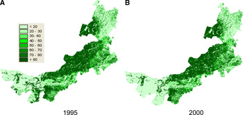
Mapping the grassland resources of China illustrates why we need to narrow the focus of our study. According to satellite imagery from all of China, there are more than 4,000,000 km2 of grasslands, covering above 40 per cent of the nation's total area. Using all of these data would mean working with at least 4,000,000 observations, which would be computationally burdensome. Therefore we restrict our attention to the case of Inner Mongolia (figure 1). With the exception of the more remote areas of China's far west, the grasslands in Inner Mongolia are the most abundant in China. Inner Mongolia's grasslands account for 18 per cent of China's total grassland area. They also are by far the most economically important grasslands in China; much of the area in Tibet and Xinjiang is not used for raising livestock and population densities are low. Within Inner Mongolia, the area covered by grasslands accounts for 31 per cent of the total area.
Grassland cover in (a) 1995 and (b) 2000 in Inner Mongolia.

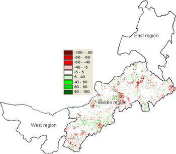
However, even if we just restricted our attention to this one province, we would still have to deal with a large (potentially unwieldy) sample of more than 1,000,000 observations (the total area of the province is 1,143,314 km2). Because of this, we decided to restrict our attention further to a specific region of Inner Mongolia. Traditionally, the province can be broken into three regions – the western zone, the middle zone and the eastern zone (figure 2; China Agricultural Zoning Committee (1989)). Since the western zone, which is mostly desert, contains less than 10 per cent of the province's grassland (see Supplementary appendix 2, table A1, row 4 online), and the eastern zone, which traditionally was part of the northeastern agricultural belt (that is, it is in many respects more like Heilongjiang and Jilin provinces than the rest of Inner Mongolia), only contains about 20 per cent of the province's grassland (see Supplementary appendix 2, table A1, row 3 online), we decided to focus on the middle zone. It should be noted that within the middle grassland region in 1995, 50.4 per cent of the grassland is Dense grassland cover, 36.4 per cent of the grassland is Moderate grassland cover, and 13.2 per cent of the grassland is Sparse grassland cover.
Spatial heterogeneity in the changes in grassland cover in each 1 km2 in the Middle Grassland Zone of Inner Mongolia in the period between 1995 and 2000.

2.2 Data for explanatory variables: roads and other factors
The basic data for our roads variable come from provincial, county and local maps from the CAS data center. The maps are up to date through 1995. The information from hard copies of the maps was digitized by a CAS working group in 1999 and 2000. Although it would be simple to calculate the straight-line distance from each pixel to the nearest segment of digitized road, such an approach is likely to provide a misleading measure of road access. More than half of Inner Mongolia's land area is grassland growing on rolling hills that are punctuated by gullies, valleys and canyons. In such an environment, a realistic measure of accessibility requires knowledge of the topography and, in particular, of watersheds. Our assumption is that travel within a watershed is likely to be less impeded than travel between watersheds. Hence, if a road enters a watershed, all pixels within that watershed are likely to have relatively easier access to the road.Footnote 4
A second issue also arises concerning what is the appropriate unit into which we should divide our data. Should we use administrative boundaries such as counties, or should we use natural boundaries such as watersheds? It is plausible that settlement and grazing decisions are influenced by grass quality (or some other cross-watershed policy or economic force) at a larger scale than the pixel level. Planning of large roads is also likely to occur at a much larger scale than the pixel. There are also many other factors that suggest that natural watershed boundaries are more appropriate than administrative boundaries. This is especially true considering that the boundaries of watersheds reflect the inherent winding line of a watershed in which all the natural conditions of land use and human development activities share the same characteristics. Because of this, local governments almost always use watersheds (instead of administrative boundaries) when undertaking environmental or development planning. Therefore, it seems natural to use the boundary of watersheds as the analytical units in this study.
2.2.1 Creating the road variables
As a result of these two issues, we developed a three-step procedure to take the digitized road map of the province and turn it into a discrete, pixel-specific measure of the largest road that penetrates any part of each watershed. The first step began with a detailed GIS map of Inner Mongolia. We used this map plus information on elevation and the watershed delineation function in ArcGIS to divide the area of the province into distinct, non-overlapping watersheds. The boundaries of watersheds for the middle zone are shown in figure 3.Footnote 5
Boundaries of watersheds (n = 5, 729) in the Middle Grassland Zone of Inner Mongolia.

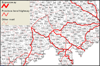
In step two, the digitized road map and the digitized watershed map were merged.Footnote 6 Representations of the watershed maps overlaid with the road network are shown in figure 4. This merging was a key step which allowed each watershed to be assigned to one of four categories, according to the size of the largest road that runs through the watershed (see Supplementary appendix 3 online). The four types of roads are: expressways (multilane, controlled access highways); province-level highways (major roads which are typically not controlled access but usually relatively well maintained since the province's highway bureau is charged with their maintenance); other roads (all major roads except expressways and province-level highways); and no roads (watersheds with no major roads – or those with only smaller and village-level roads). After this step every watershed in the province is labeled with one (and only one) of four names: expressway watershed; province-level highway watershed; other road watershed; or no road watershed. If a watershed has an expressway and a province-level highway (and/or other road) inside its boundary it is still, by definition, an expressway watershed.
Example of boundaries of watersheds overlaid with the road network in the Middle Grassland Zone of Inner Mongolia in 1995.

The final step assigns all of the pixels in the same way as the watersheds. This, of course, means that each of the 563,296 pixels in the middle zone of Inner Mongolia has one of four designations: expressway pixel, province-level highway pixel, other road pixel, or no road pixel.
2.2.2 Other control variables
In addition to information on the grasslands and roads, other data are used to create variables to control for other factors that determine grassland quantity and quality. When looking at the empirical literature on the determinants of grassland cover, we find four broad categories of variables. Ding et al. (Reference Ding, Niu and Yang2006) and Zheng et al. (Reference Zheng, Xie, Robert, Jiang and Shimizu2006) and others include a number of geographic and climatic variables. Han et al. (Reference Han, Zhang, Wang, Bai, Wang, Han and Li2008), Rozelle et al. (Reference Rozelle, Huang and Zhang1997), and Williams (Reference Williams2007) include demographic and economic variables. Other authors (e.g., Zhang et al., Reference Zhang, Liu, Bai, Shen, Yan, Ding, Li and Zheng2006) include measures of distance from the grassland plots to different features (such as distance to the nearest city). Different authors also consider other factors such as whether or not the pixel is in a protected area (Tilman et al., Reference Tilman, Polasky and Lehman2005). In order to make our analysis as consistent as possible with the rest of the literature, we have collected information on four sets of variables: geographic and climatic factors, demographic and economic factors, measures of distance, and other factors. A number of these factors have been consistently found to causally affect grassland degradation in the review paper by Trombulak and Frissell (Reference Trombulak and Frissell2000).
To generate the control variables for our analysis, we draw on data and information from a number of different sources. The data for measuring rainfall (measured in mm per year) and temperature (measured in accumulated degrees centigrade per year) are from the CAS data center but were initially collected and organized by the Meteorological Observation Bureau of China from more than 600 national climatic and meteorological data centers. For use in our study, we take the point data from the 15 climate stations in Inner Mongolia and interpolate them into surface data using an approach called the thin plate smoothing spline method (Hartkamp et al., Reference Hartkamp, De Beurs, Stein and White1999). The elevation and terrain slope variables, which measure the nature of the terrain of each county, are generated from China's digital elevation model data set that is part of the basic CAS database. Information on the properties of soil is also part of our set of geographic and climatic variables from the CAS data center. Originally collected by a special nationwide research and documentation project (the Second Round of China's National Soil Survey) organized by the State Council and run by a consortium of universities, research institutes and soils extension centers, we use these data to specify 10 variables: the nitrogen, phosphorous and potassium content of the soil (measured as percentage); available phosphorous and available potassium in the top soil (measured in ppm); soil pH value; soil clay, soil loam and soil sand (denoting the proportion of clay, loam and sand in the soil (measured as percentage); and organic matter in the top soil (measured as percentage). By using a conventional Kriging algorithm (Kravchenko and Bullock, Reference Kravchenko and Bullock1999), we are able to interpolate the soil information into surface data to get more disaggregated information on the property of the soil over space for each pixel.
Two demographic and economic variables, population and the level of gross domestic product per km2 (GDP), are included in our modeling work. The demographic data for 1995 and 2000 are from the Population Statistical Yearbook for China's Counties. Information on GDP for each county for 1995 and 2000 is from the Socio-economic Statistical Yearbook for China's Counties (NBSC, 2001). When there are missing data in the yearbook, the information is supplemented by the province's annual statistical yearbook for 1995 and 2000. In order to get pixel-specific measures of the demographic variables we use an approach called the Surface Modeling of Population Distribution framework (Yue et al., Reference Yue, Wang, Liu, Chen, Qiu, Deng, Liu, Tian and Su2005; Deng et al., Reference Deng, Su and Zhan2008b) to interpolate the data across space (measured as persons/km2). The level of GDP (GDP per km2) is also interpolated across space using commonly available GIS algorithms (Doll et al., Reference Doll, Muller and Elvidge2000, Reference Doll, Muller and Morley2006; Deng et al., Reference Deng, Su and Zhan2008b).
We also created several measures of distance (in km), defined separately for each pixel in our sample. The variable, distance to nearest road, measures the distance from each grid cell to the nearest road of any type. Distance to the provincial capital measures the distance (by the shortest road route) from each pixel to Hohhot, Inner Mongolia's provincial capital. We also generated a variable, distance to the nearest urban core, which is the shortest road route from each pixel to the nearest county seat or other major urban center.
Finally, we also obtained data for several other factors. For example, we create a variable, bufferfarmland, to identify if a pixel is surrounded by cultivated area. The idea of including this variable is to hold constant any impact on the grassland that could arise if a pixel of grassland is near an area in which agriculture is being practiced. The variable is created by measuring the percentage of the area that is being cultivated within 10 km of the pixel of interest. Similarly, we create a variable, bufferforest, to identify if a pixel is surrounded by forested area. Finally, we also include a variable called grassland area in 1995. This variable seeks to hold constant the quality-adjusted quantity of grassland in the initial period of our analysis (measured as QA-Grassland 1995). Table A2 in Supplementary appendix 4 online reports the variable name, units, number of observations, mean and standard deviation for all variables used in the paper.
3. Approach to estimate the multivariate effect of roads on grasslands
The basic empirical relationship that we are interested in is:

where Grassland i, t is measured in one of two ways. In one set of regressions, it is the area of the grasslands in pixel i in year t = 2000. In the other set of regressions it is the change of the area of the grassland in pixel i between 1995 and 2000. This is discussed further below. In addition, because of differences within and across pixels in the quality of grasslands, we replace Grassland with the quality-adjusted measure of grassland area, QA-Grassland.
The explanatory variable of interest, (Access to Roads)i, t−j, is a measure of the nature of the largest road that ran through the watershed which contains pixel i in year t − j (which in our study is 2000 − 5 = 1995) and a 1 is our coefficient of interest. We use a lagged measure of roads (lagging it by 5 years) to help reduce concerns about endogeneity, since changes in grassland cover between 1995 and 2000 (or the level of the grasslands in 2000) should have no direct effect on the road network in 1995.
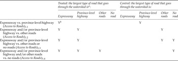
Since we are interested in the impact of whether there is a road in the watershed (or not) as well as the type of road (expressway vs. province-level highway vs. other road), we define Access to Roads i, t−j in four different ways. In model 1.1, we include in our sample only the expressway and province-level highway pixels, and (Access to Roads)1.1, i, t−j will equal 1 if the pixel is an expressway pixel and 0 if the pixel is a province-level highway pixel. Note, the other road pixels and no road pixels are excluded from the analysis when we use (Access to Roads)1.1, i, t−j. In the estimation of model 1.1, a 1.1 will measure the effect on the grassland area of changing a highway system from a province-level highway to an expressway.
In model 1.2, we include in our sample only the expressway, province-level and other road pixels, and Access to Roads 1.2, i, t−j will equal 1 if the pixel is either an expressway pixel or a province-level highway pixel and 0 if the pixel is a ‘other road pixel’. In the estimation of model 1.2, a 1.2 will measure the effect on the grassland area of changing a highway system from some other road to either a province-level highway or to an expressway. The roadless pixels are dropped from the analysis when we work with model 1.2.
In models 1.3 and 1.4 we use the full sample (that is all of the pixels in the middle zone of Inner Mongolia). The empirical exercise in model 1.3 is like that of model 1.2, except we set Access to Roads 1.3, i, t−j = 0 when the pixels are either other road pixels or no road pixels. In that way, the interpretation of a 1.3 becomes the effect on the grassland area of changing a highway system from some other road to either a province-level highway or to an expressway, or of building a province-level highway or expressway into a previously roadless watershed. In model 1.4, we set Access to Road 1.4, i, t−j = 1 if there is any type of road in the watershed, and set it to 0 if there is no road in the watershed. The interpretation of a 1.4 becomes the effect on the grassland area of building any type of road into a previously roadless watershed. Table 1 summarizes the different ‘experiments’ that are conducted by estimating models 1.1–1.4.
Definition of Access to Roads variables

aIf the largest type of road that goes through the watershed is expressway, the watershed may also contain province-level highway or other roads. Likewise, if the largest type of road is province-level highway, it may also include other roads.
bY denotes that this largest type of road goes through the watershed.
The estimation of a 1 using equation (2), of course, is problematic for several reasons. Pixels in watersheds with expressways are likely to differ from those in watersheds without any roads (or with only minor roads) in many ways. They may have easier topography and more productive soils along with a number of unobserved locational advantages, since richer areas (or areas with more development potential) are more likely to attract investment in roads. Hence, applying OLS to equation (2) is unlikely to give unbiased treatment effects estimates of what happens to the grassland cover when a previously roadless watershed has new roads introduced (or existing roads upgraded). Indeed, as discussed above, previous work (Zhang et al., Reference Zhang, Liu, Bai, Shen, Yan, Ding, Li and Zheng2006) suggests many other factors that might affect grassland area and since some are likely to be correlated with both grassland area and access to roads, we can reduce omitted variable bias by controlling for as many variables as possible. This gives the model:

Where, in addition to the variables and parameters in equation (2), equation (3) includes the matrix Z. In our analysis Z includes 14 measures of geographic and climatic variables (elevation, terrain slope, nitrogen, phosphorous, potassium, available phosphorous, available potassium, soil pH value, soil clay, soil loam, soil sand, organic matter, temperature and rainfall); two measures of demographic and economic variables (population and GDP); three measures of distance variables (distance to the nearest road, distance to the provincial capital and distance to the nearest urban core); and two other variables (bufferfarmland and bufferforest). In versions of the equations in which the dependent variable is the change in the grassland (from 1995 to 2000), we also include an additional variable that holds constant the level of the grassland in 1995 (Grassland area in 1995). Since most of the 22 variables in Z – all except population, GDP, bufferarea10 and distance to the nearest urban core – only vary across space, we only include an i subscript on Z.
3.1 Matching methodology
As in the case of our OLS models (in equations (2) and (3)), the matching method is another way to examine the impact of a treatment (in our context, existence of particular types of roads) on an outcome (in our case, grassland) when selection takes place on observable characteristics (Rosenbaum and Rubin, Reference Rosenbaum and Rubin1983; Dehejia and Wahba, Reference Dehejia and Wahba2002). Estimating the effect of roads on grassland cover without bias using the matching method assumes that the outcome in the base state (grassland if the pixel was not in a watershed with a particular type of road) is independent of the treatment, conditional on observed covariates Z. In other words, for pixels within subgroups defined by Z, being located in a watershed with roads is unrelated to what the grassland cover would be if the pixel were not in a watershed with roads. This is the so-called Conditional Independence Assumption. If this assumption holds, we can say that, given the observable covariates, the grassland cover of the control pixels is what the grassland cover of the treated pixels would have been had the road (or had the larger road) not penetrated into the watershed of the treatment pixel.
Unlike OLS, however, matching works by finding a control pixel that is very similar to the treatment pixel by conditioning on Z variables non-parametrically rather than linearly (Black and Smith, Reference Black and Smith2004). To take advantage of the matching method, we follow the recent literature and match every treated pixel with a control pixel using the Covariate Matching estimator developed by Abadie and Imbens (Reference Abadie and Imbens2006). With Covariate Matching we estimate the average treatment effect on the change in grassland cover by comparing outcomes between treated observations (pixels in a watershed with a specific type of road), and control observations (pixels in a watershed without the specific type of road). In our analysis, we choose to match the two nearest neighbors with the same (similar) covariates (Z), where the variables in Z are the same as in equation (3). Within this set of pixels, we can then directly estimate E(Y i1 | T i = 1, Z i) and E(Y i0 | T i = 1, Z i). This approach means that once we have a matched sample, we compare the grassland of the treated pixel with the grassland of the control pixel. One additional advantage of Covariate Matching is that it allows us to correct for the bias caused by the matching discrepancy. To minimize geographic mismatch, we enforce exact matching by prefecture; that is, only pixels from the same prefecture are allowed to be matched. The exact matching helps control for unobserved heterogeneity at the prefecture level (e.g., policy environment). With covariate matching, we report the results using the Mahalanobis metric weighting scheme.
Using the method of matching also has the additional advantage of alleviating spatial issues. The basic unit of observation in our study is the 1 km2 pixel, of which there are 563,296 in the middle zone of Inner Mongolia. When using such data there is a high correlation in grassland cover between neighboring pixels (as well as lesser – but still statistically significant – correlation in the residuals of the OLS estimates of equation (3).Footnote 7
When estimating the relationship between access to roads and the grassland this spatial autocorrelation can lead to inefficiency and invalid hypothesis testing procedures (Anselin, Reference Anselin2001). Matching methods should eliminate most of the spatial autocorrelation because every treated pixel is matched with a control pixel from a different watershed. Except for the extreme case where the two matched pixels share a common watershed boundary, the pixels are unlikely to be adjacent neighbors.Footnote 8
3.2 Two definitions of the dependent variable: grassland and change in grassland
As discussed above, we have two dependent variables of interest. Many studies of roads and grassland degradation use cross-sectional data on grassland area. However, such a cross-section may merely illustrate the correlation between where roads and grasslands are (i.e., which areas are more remote and which areas are more developed). To estimate the causal impact of roads on grasslands, one would want to look at the changes in grassland. Fortunately, as discussed above, we have two years of land use data for each pixel in Inner Mongolia. Therefore, in the rest of our analysis, we report estimates for all of the models using two dependent variables – grassland area in 2000, and the change in the grassland area between 1995 and 2000.
3.3 Accounting for heterogeneous effects
As discussed above, across pixels and within pixels the quality of grassland varies. In fact, although total grassland cover and quality-adjusted grassland cover decline between 1995 and 2000, the same is not necessarily true for the rates of change for Dense, Moderate and Sparse grasslands change. While the area of Dense grassland did fall (as did quality-adjusted grassland), moderate canopy grassland showed almost no change. At the same time, Sparse grassland actually rises over time. Because of these differences among types of grassland, in the analysis we look separately at the effect of access to roads on quality-adjusted, Dense, Moderate and Sparse grasslands.
4. Results
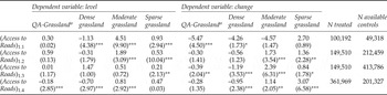
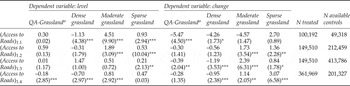
If we were to use a traditional OLS approach and control for covariates (that is, if we estimated our model using equation (3) to analyze the effect of roads using an aggregate measure of the grassland resource (QA-Grassland), the results would suggest that roads lead to grassland degradation (table 2, columns 1 and 6).Footnote 9 In fact, regardless of our measure of the access to roads (Access to Roads 1.1, 1.2, 1.3 and 1.4), after holding constant the effect of 21 other control variables, the level of the grassland in 2000 is shown to be lower in areas with roads or in areas in which there are larger or more improved roads (column 1, rows 1–4). The t-ratios associated with the Access to Roads variable in all of the equations suggest that the estimated effects are significantly different from zero.
Pixel-specific impacts of roads (1995) on the level of grassland (2000) and the changes in grassland (between 1995 and 2000) for the Middle Grassland Zone of Inner Mongolia, China, based on the OLS estimation with covariatesa

Notes: Results of t-tests for the difference in the mean change between treatment and control groups are reported with asterisks.
*denotes significance level at 10%; **denotes significance level at 5%; ***denotes significance level at 1%.
a In this table we report only the coefficients for the variable of interest (access to roads). If the reader is interested in examining the full regressions (with all of the coefficients and goodness of fit statistics), please see tables A3 – A6 in Supplementary appendix 5 online.
bQuality-adjusted grassland area is calculated as 0.75 × (Dense grassland area) + 0.35 × (Moderate grassland area) + 0.125 × (Sparse grassland area).
Roads are also shown to be associated with grassland degradation when we measure the degradation effect as the change in the grassland between 1995 and 2000 (that is: QA-Grassland2000 – QA-Grassland1995 – table 2, column 6). As in the case of the regression when using the 2000 level of the grassland, regardless of the way we measure access to roads (1.1, 1.2, 1.3 or 1.4), the sign on the Access to Roads variable is negative (rows 1–4). The coefficient is statistically significant in three of the four versions of the regression (all except row 3 for Access to Road1.3). According to this traditional approach of analyzing the effect of roads on grasslands, roads lead to grasslands degradation. In all of the eight regressions (using the two measures of the dependent variable and the four measures of the independent variable of interest), the sign on the Access to Roads variable is negative; it is statistically significant in seven of the cases.
The importance of using a better strategy to control for the covariates by using a Covariate Matching approach is evident when comparing the results from table 2, columns 1 and 6 (the results from the OLS estimation) and the results from table 3, columns 1 and 5 (the results from the Covariate Matching approach). This is especially true when we look at the results of the Covariate Matching approach that seek to estimate the effect of roads in 1995 on the level of the aggregate grasslands in 2000 (QA-Grasslands2000). The signs on the Access to Roads variable (1.1, 1.2 and 1.3) actually change (from negative to positive), although the t-ratios are small in all of the cases. Only in the final regression (measuring the effect of Access to Roads1.4 in 1995 on QA-Grasslands2000) is the sign negative and statistically significant. The magnitude of the coefficient, however, is much smaller in table 3 (column 1, row 4) than in table 2 (column 1, row 4). Moreover, although the signs on all four of the coefficients of the Access to Road variable in the set of Covariate Matching regressions that use the change in the grasslands between 1995 and 2000 are still negative, only two of the four are statistically significant. Therefore, our degree of confidence in the claim that our estimates demonstrate that roads negatively affect grasslands must necessarily be lower when we move from a traditional OLS approach to one using Covariate Matching that is better suitable for analyzing the treatment effect.
Pixel-specific impacts of roads (1995) on the level of grassland (2000) and the changes in grassland (between 1995 and 2000) for the Middle Grassland Zone of Inner Mongolia, China, based on Covariate Matching estimation with covariates

Note: Results of t-tests for the difference in the mean change between treatment and control groups are reported as asterisks: *significant at 10%; **significant at 5%; ***significant at 1%.
aQuality-adjusted grassland area is calculated as 0.75 × (Dense grassland area) + 0.35 × (Moderate grassland area) + 0.125 × (Sparse grassland area).
4.1. Roads and the grassland: when grassland quality is considered
If the above exercises suggest that using Covariate Matching is important, the results using our measures of grasslands disaggregated by quality (regardless of whether or not we used OLS or Covariate Matching) demonstrate that it is even more important to estimate the regressions separately with measures of Dense grassland cover; Moderate grassland cover and Sparse grassland cover as the dependent variables (tables 2 and 3, columns 2–4 and columns 6–8). Specifically, when using OLS estimation with covariates (table 2), we can see how our results change completely when we estimate the effect of Access to Roads on the level of Dense grassland cover (column 2) compared to the case when we estimate the effect of Access to Roads on the level of Sparse grassland cover (column 4). The same is true when examining the difference between the effects of Access to Roads on the change in Dense grassland cover compared with the change in Sparse grassland cover (columns 6 and 8). In the case of all Access to Roads measures, the sign on the coefficient is negative (and significant in seven of eight regressions) when looking at the effect of roads on high quality grassland (Dense grassland). In contrast, in the case of all Access to Roads measures, the sign on the coefficient is positive (and also significant in seven of the eight regressions) when looking at the effect of roads on low quality grassland (Sparse grassland). In other words, our results suggest that roads are leading to the degradation of Dense grassland cover while at the same time (in other places) roads are associated with the restoration of Sparse grassland cover.
The exact same story is found when examining the difference in the effect of roads on Dense and Sparse grassland cover using Covariate Matching (table 2, columns 2 and 4, 6 and 8). In all of the regressions that examine how the Access to Roads variables affects Dense grassland cover, the signs are negative (and significant in five of the eight regressions). The findings are the exact opposite in the case of low quality grasslands. In all of the regressions that examine how the Access to Roads variables affects Sparse grassland cover, the signs are positive (and significant in six of the eight regressions). Clearly, whether we use OLS or Covariate Matching, we find sharply varying effects of roads on the grasslands, depending on the quality of the resource.Footnote 10
Does this necessarily mean that roads are good for Sparse grassland land cover? In fact, because of the possibility that there are shifts of grassland among the three types of grassland due to Access to Roads, the estimated parameters for Access to Roads in the three equations may include two parts. First, it could be that roads are generating more Sparse grassland cover or more Moderate grassland cover. Second, and less inherently positive, it could be that roads are degrading Dense and Moderate grassland cover and this is why Sparse grassland cover is rising. Unfortunately, we are not able to separate the different nature of the shifts of land among three grasslands and between grassland and other land, given the data we have. The reader needs to remember this caveat when interpreting the results.
5. Conclusion and discussion
In this paper we have sought to estimate the impacts of roads on grassland in the middle region of Inner Mongolia. However, our paper goes further and shows the importance of the choice of methodology and modeling in analyzing the estimated effects. In particular, we found that using Covariate Matching was important in reducing potential bias, due to the non-parametric nature of the matching estimation and the correction of matching discrepancies in the matching procedure, while the OLS estimates produced a set of results that were fairly convincing in showing the negative effect of roads on the overall nature of the grassland resources.
Above all, however, we found that it was even more important to disaggregate the quality of resource when estimating the impact on roads. Regardless of our estimation approach, we found that roads appear to have a negative and significant effect on grasslands degradation in areas where the resource is high in quality (that is, in regressions with Dense grassland cover as the dependent variable). In contrast, roads lead to higher levels of the grassland when resources are relatively lower quality. While this could be shifts from Dense and Moderate grassland that is deteriorating, it might also be a sign that restoration is occurring. Hence, accounting for the heterogeneous nature of the resource can completely change the estimated relationship and could make a big difference in any policy analysis that would rely on the estimates.
So why might we see these polar results in areas with Dense grassland cover and Sparse grassland cover? While it is beyond the scope of this paper to identify the exact mechanism, logically one could imagine that these results are plausible. When roads penetrate into (or are improved in) areas with high quality grasslands, it may intensify efforts to exploit the resource – which is worth exploiting, given its high quality. This is indeed what may be happening in the areas with significant amounts of Dense grassland cover. According to provincial level statistics (MOA, 2009), mutton production rose by more than 10 times between the 1980s and 2008. However, when roads enter into areas with low quality (previously degraded?) grass, assuming that there is restoration at work, it is possible that roads can be used as an avenue of escape (and allow people to move out of the grassland areas for working and living). Two distinctive trends in Inner Mongolia would support such an interpretation. First, while in the 1980s there was almost no dairy production in Inner Mongolia, by 2008 there were significantly more dairy cows than sheep (MOA, 2009). Dairy cows in Inner Mongolia are almost all raised in penned environments and would have distinctly less impact on the grassland. Second, migration across China, including from Inner Mongolia, has risen rapidly during the 1990s and 2000s (Huang et al., Reference Huang, Zhang, Li and Rozelle2009). It is also possible that new roads into such areas would allow other non-grass-based enterprises/industries to enter into the grasslands and divert the attention from grass-based activities to non-grass-based activities. Further research is needed to more fully understand the behavioral dynamics underlying our econometric findings.
In the same vein, it is important to bear in mind that decline in grassland in the areas with rich and high quality grassland on the one hand, and improvement in the sparsely covered grassland on the other, cannot be treated as canceling each other out. The two may have fairly distinct implications for the environment and ecology. Hence, future work on the value of the ecosystem services that are destroyed and/or created needs to proceed, work that would allow policy makers to better judge and measure the full impact of roads.
Supplementary materials
The supplementary materials referred to in this article can be found online at journals.cambridge.org/ede.