


1. Introduction
Large deviations are used extensively in physics (thermodynamics, statistical mechanics) as well as in mathematics (information theory, stochastic analysis, mathematical finance) to estimate the exponential decay of probability measures of rare events. Varadhan [Reference Varadhan52], Schilder [Reference Schilder49], and Freidlin and Wentzell [Reference Freidlin and Wentzell25] proved, with different degrees of generality, large deviations principles (LDPs; in ℝn and on path space) for solutions of stochastic differential equations with small noise, and the monographs by Dembo and Zeitouni [Reference Dembo and Zeitouni16] and Deuschel-Stroock [Reference Deuschel and Stroock19] provide a precise account of those advances (at least up to the mid-1990s). In the past decade, this set of techniques and results has been adopted by the mathematical finance community: finite-dimensional large deviations (in the sense of Gärtner-Ellis) have been used to prove small- and large-time asymptotics of implied volatility in affine models [Reference Forde, Jacquier and Lee22, Reference Jacquier, Keller-Ressel and Mijatović34], sample-path LDP (à la Freidlin–Wentzell [Reference Freidlin and Wentzell25]) have proved efficient for determining importance sampling changes of probability [Reference Genin and Tankov31, Reference Guasoni and Robertson32, Reference Robertson48], and heat kernel expansions (following Ben Arous [Reference Ben Arous9] and Bismut [Reference Bismut11]), have led to a general understanding of small-time and tail behaviour of multi-dimensional diffusions [Reference Baudoin and Ouyang5, Reference Baudoin and Ouyang6, Reference Deuschel, Friz, Jacquier and Violante17, Reference Deuschel, Friz, Jacquier and Violante18]. These asymptotics have overall provided a deeper understanding of the behaviour of models, and, ultimately, allow for better calibration of real data; a general overview can be found in [Reference Pham46].
Motivated by financial applications, we derive here asymptotic small-time and tail behaviours of the solution to a generalised version of the Stein–Stein stochastic volatility model, originally proposed in [Reference Schöbel and Zhu50, Reference Stein and Stein51]. We in particular consider two important (in light of the recent trends in the literature-proposed models) extensions: (i) the stochastic differential equation (SDE) driving the instantaneous volatility process is started from a random distribution; this so-called ‘randomised’ type of model was recently proposed in [Reference Jacquier and Roome38, Reference Jacquier and Shi39, Reference Mechkov41], in particular to understand the behaviour of the so-called ‘forward volatility’; (ii) the volatility process is driven by a fractional Brownian motion. Fractional stochastic volatility models, originally proposed by Comte and Renault [Reference Comte and Renault14, Reference Comte, Coutin and Renault15] with H ∈ (1/2, 1), have recently been extended to the case H ∈ (0, 1/2), and a recent flourishing activity in this area [Reference Alô’s, Leòn and Vives3, Reference Bayer, Friz and Gatheral7, Reference Fukasawa26, Reference Gatheral, Jaisson and Rosenbaum30, Reference Jacquier, Martini and Muguruza35] has established these models as the go-to standards for estimation and calibration.
The original motivation behind randomisation of the initial starting point is rooted in financial practice, where only the initial value of the stock price process is observed directly and the instantaneous value of volatility is subject to calibration. The effect of randomisation of the initial volatility on the implied volatility surface was explored by Jacquier and Roome [Reference Jacquier and Roome37] in a simple ‘random environment’ setting, where the volatility component was assumed to follow constant elasticity of variance dynamics. Their results provide progress on both theoretical and practical levels: they solve a practical modelling problem in a simple tractable setting and at the same time raise awareness of the potential prowess of applying random evolution equations for financial modelling. In this paper we follow up on this direction and blend more involved approaches (proposed by [Reference Mellouk42, Reference Millet, Nualart and Sanz43]) from the literature around random environment and random evolution equations into our financial model, where randomness also appears in the drift and diffusion coefficients of the process. On the practical level, independently from the results of [Reference Jacquier and Roome37], Mechkov [Reference Mechkov41] goes a step further in endorsing the idea of randomising the initial volatility and makes a strong case to move away from modelling hidden variables (such as stochastic volatility) in the traditional way. He argues that starting the volatility from a fixed starting point heavily underestimates the effect of the hidden variable on the slope of the implied volatility smile, and therefore ‘hot start’ volatility models (with random starting point) significantly outperform traditional ones. Indeed, both randomised models [Reference Jacquier and Roome37, Reference Mechkov41] produce the desired explosion in the smile at short maturities. Jacquier and Shi [Reference Jacquier and Shi39] develop this further by providing a precise link between the rate of explosion of implied volatilities on the short end and the tail distribution of the initial distribution of the volatility process in a ‘randomised’ Heston model. These outputs confirm that stochastic volatility models with a random starting point constitute a class of counterexamples to the long-standing belief, formulated by Gatheral [Reference Gatheral29, Chapter 5], that jumps in the stock price process are needed to produce steep short-dated implied volatility skews. Another example of broadly different design was provided by Caravenna and Corbetta [Reference Caravenna and Corbetta12]. In their ‘multiscaling’ model, the stock price process is continuous, while the volatility process has (carefully designed) jumps, and steepness of the smile is achieved with a heavy-tail distribution of the small-time distribution of the volatility. Rough fractional volatility models (with continuous volatility paths) have recently been proposed, and are able to capture the volatility skew [Reference Alô’s, Leòn and Vives3, Reference Bayer, Friz and Gatheral7, Reference Bayer8, Reference El Euch, Fukasawa and Rosenbaum20, Reference Forde and Zhang23, Reference Fukasawa26, Reference Gatheral, Jaisson and Rosenbaum30, Reference Gulisashvili, Viens and Zhang33, Reference Jacquier, Pakkanen and Stone36]. In this paper we analyse the combined effect of a rough fractional Brownian driver (with Hurst parameter H ∈ (0, 1)) in the volatility and a random starting point. We quantify how the tail behaviour (parametrised by a scaling coefficient b > 0) of the random starting point modulates the rate of explosion in the implied volatility in the presence of rough fractional volatility. Finally, in a specific simplified setting we highlight how our model blends naturally into the setting of forward-start options in stochastic volatility models, whose asymptotic properties have been studied in [Reference Jacquier and Roome38]. In proving our results, we improve the large deviations literature on both SDEs with random starting points and fractional SDEs.
In Section 2 we recall some concepts that will be used in the paper and set the notation. We also introduce the model (2.5), and the main assumptions on its dynamics and on the initial random starting point. Section 3 collects the main large deviations estimates in different regimes: tail behaviour (Section 3.1) and small-time behaviour (Section 3.2). In each case we present two different scenarios consisting of an appropriately rescaled fractional model (Theorems 3.1 and 3.4) and a simplified diffusive model (Theorems 3.3 and 3.6) with more restrictive conditions on the random starting point (allowing for simpler large deviations rate functions). Section 4 displays applications to implied volatility asymptotics (Corollaries 4.1 and 4.2), and presents an application to forward-start options. Proofs can be found in the appendix.
2. Setup and notation
As outlined in the introduction, we prove pathwise large deviations for a two-dimensional system generalising the Stein–Stein model [Reference Schöbel and Zhu50, Reference Stein and Stein51], with random initial datum. In particular, via suitable rescaling, we determine the small-time and the large-tail behaviours of the system. Before delving into the core of the paper, let us recall some useful facts about large deviations and Gaussian processes, which shall also serve as setting the notation for the rest of the paper. Unless otherwise stated, we always work on a finite time horizon, say [0, 1] without loss of generality, which we denote by 𝒯, and we write 𝒯 * := 𝒯 \{0}. We let 𝒞 := 𝒞(𝒯, ℝ) be the space of continuous functions from 𝒯 to ℝ, and 𝒞 2b the space of twice-differentiable functions on 𝒯 with bounded partial derivatives up to the second order. We write Xε ~ LDP(hε, I) when the sequence (Xε)ε>0 satisfies a large deviations principle (Definition 2.2) on 𝒞, as ε tends to zero with good rate function I and speed hε, where hε denotes a function satisfying limε↓0 hε = 0. For a random variable X, we denote by supp(X) its support.
2.1. Large deviations and fractional Brownian motion
We use [Reference Dembo and Zeitouni16] as our guide through large deviations. Given a topological space 𝒳 and its completed Borel σ -field ℬ 𝒳, for any A ∈ ℬ 𝒳 we denote by A and Ā respectively its interior and closure, and consider a sequence (Xε)ε>0 on (𝒳, ℬ 𝒳).
Definition 2.1. A (good) rate function is a lower semi-continuous mapping I : 𝒳 → [0, ∞] such that any level set {x : I(x) ≤ z} is a closed (compact) subset of 𝒳, for z ≥ 0.
Definition 2.2. The sequence (Xε)ε>0 satisfies a large deviations principle (LDP) on (𝒳, ℬ 𝒳) as ε tends to zero, with speed hε and rate function I, if for any Borel subset A ⊂ 𝒳, the following inequalities hold:
 $$ - \mathop {\inf }\limits_{{A^o}} I(\varphi ) \le \mathop {\liminf}\limits_{\varepsilon \downarrow 0} {h_\varepsilon }\log {\rm {P}}({X^\varepsilon } \in A) \le \mathop {\limsup }\limits_{\varepsilon \downarrow 0} {h_\varepsilon }\log {\rm {P}}({X^\varepsilon } \in A) \le - \mathop {\inf }\limits_{\overline A } I(\varphi ).$$
A particularly convenient tool to prove large deviations is so-called exponential equivalence, which we recall from [Reference Dembo and Zeitouni16, Definition 4.2.10] as follows:
Definition 2.3. On a metric space (𝒴, d), two 𝒴-valued sequences (Xε)ε>0 and  ${({\tilde X^\varepsilon })_{\varepsilon > 0}}$ are called exponentially equivalent (with speed hε) if there exist probability spaces (Ω, ℬε, Pε)ε>0 such that for any ε > 0, Pε is the joint law and, for each δ > 0, the set
 $\{ \omega {\kern 1pt} :{\kern 1pt} ({\tilde X^\varepsilon },{X^\varepsilon }) \in {\Gamma _\delta }\} $ is ℬ ε-measurable, and
 $$\mathop {\limsup }\limits_{\varepsilon \downarrow 0} {h_\varepsilon }\log {{\rm {P}}^\varepsilon }({\Gamma _\delta }) = - \infty ,$$
where  ${\Gamma _\delta }{\kern 1pt} : = {\kern 1pt} \{ (\tilde y,y){\kern 1pt} :{\kern 1pt} d(\tilde y,y) > \delta \} \subset {\cal Y} \times {\cal Y}$.
Theorem 2.1. Let (Xε)ε>0 and  ${({\tilde X^\varepsilon })_{\varepsilon > 0}}$ be two exponentially equivalent sequences (with speed hε) on some metric space. If (Xε) ~ LDP(hε, ΛX) for some good rate function ΛX, then
 $({\tilde X^\varepsilon }) \sim LDP({h_\varepsilon },{\Lambda ^X})$
The last tool we shall need repeatedly is the following contraction principle [Reference Dembo and Zeitouni16, Theorem 4.2.1]:
Theorem 2.2. (Contraction principle.) Let 𝒳, 𝒴 be two topological spaces, f : 𝒳 → 𝒴 a continuous function, and I : 𝒳 → [0, ∞] a good rate function. For each y ∈ 𝒴, define I ′(y) := inf{I(x): x ∈ 𝒳, y = f (x)}. Then, if I controls the LDP associated with a family of probability measures {με} on 𝒳, then I ′ controls the LDP associated with the family of probability measures {με ∘ f −1} on 𝒴 and I ′ is a good rate function on 𝒴.
On a real, separable Banach space (ℰ, ||⋅||), we denote by ℬ the associated Borel sigma field. Letting ℰ * denote the topological dual of ℰ, we define a Gaussian measure as follows:
Definition 2.4. A Gaussian measure μ on (ℰ, ||⋅||) is such that every ϑ * ∈ ℰ *, when viewed as a random variable via the dual pairing ϑ → 〈ϑ *, ϑ〉ℰ*ℰ, is a real Gaussian random variable on (ℰ, ℬ, μ).
We associate a Gaussian process with a Gaussian measure in the usual way [Reference Carmona and Tehranchi13, Section 3.2]. Particular examples of Gaussian processes, crucial for the rest of the paper, include standard Brownian motion on the time interval 𝒯, where ℰ = 𝒞 equipped with the supremum norm and with the topology of uniform convergence, and ℰ * is the space of signed measures on 𝒯. In fact, this construction applies to all (continuous) centered Gaussian processes, which are uniquely characterised by their covariance operator. A fractional Brownian motion WH with Hurst parameter H ∈ (0, 1) is such a Gaussian process, starting from zero, with covariance
 $$\langle W_t^H,W_s^H\rangle = {1 \over 2}(|t{|^{2H}} + |s{|^{2H}} - |t - s{|^{2H}}),\quad \quad {\rm {for\,any}}\,s,t \in {\cal T}.$$
Of primary importance in understanding small-noise behaviours of Gaussian systems is the concept of reproducing kernel Hilbert spaces (RKHS), which we recall following [Reference Carmona and Tehranchi13, Definition 3.3]:
Definition 2.5. Let μ be a Gaussian measure on ℰ and define the map ℛ : ℰ * → ℰ by  ${\cal R}{x^*}{\kern 1pt} : = {\kern 1pt} \int_{\cal E} \langle {x^*},x\rangle x\mu ({\rm {d}}x)$. The RKHS ℋμ of μ is the completion of the image ℛℰ * for the norm ||ℛx *||ℋμ := (〈x *, ℛx *〉)1/2, for all x * ∈ ℰ *.
To characterise the RKHS of fractional Brownian motion, the usual tool is its Volterra representation [Reference Norros, Valkeika and Virtamo45],
 $$W_t^H = \int_0^t {K^H}(t,s){\kern 1pt} {\rm {d}}{B_s},$$
which holds almost surely for all t ∈ 𝒯, where B is a standard Brownian motion generating the same filtration as WH, and KH is the Volterra kernel defined, for any s, t ∈ 𝒯 with 0 < s < t, by [Reference Norros, Valkeika and Virtamo45, Theorem 5.2]
 $${K^H}(t,s) = \left\{ {\matrix{
{{{{\kappa _H}} \over {{s^{{H_ - }}}}}[(t(t - s{{))}^{{H_ - }}} - {H_ - }\int_s^t {{{{(u - s)}^{{H_ - }}}} \over {{u^{1 - {H_ - }}}}}{\kern 1pt} {\rm {d}}u],} \hfill & {{\rm{if}}H \lt {1 \over 2},} \hfill \cr
{{{{\kappa _H}{H_ - }} \over {{s^{{H_ - }}}}}\int_s^t {{{u^{{H_ - }}}{\kern 1pt} {\rm {d}}u} \over {|u - s{|^{1 - {H_ - }}}}},} \hfill & {{\rm{if}}H > {1 \over 2},} \hfill \cr
{1,} \hfill & {{\rm{if}}H = {1 \over 2},} \hfill \cr
} } \right.$$
with 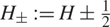 ${H_ \pm }{\kern 1pt} : = {\kern 1pt} H \pm {1 \over 2}$ and
 ${\kappa _H}{\kern 1pt} : = {\kern 1pt} {({{2H\Gamma (1 - {H_ - })} \over {\Gamma ({H_ + })\Gamma (2 - 2H)}})^{1/2}}$. For t ∈ 𝒯 *, the map KH(t, ⋅) is square integrable around the origin, and the reproducing kernel Hilbert space of the fractional Brownian motion is given by
 $${{\cal H}_{{K^H}}}{\kern 1pt} : = {\kern 1pt} \{ \int_0^t {K^H}(t,s){\kern 1pt} f(s){\kern 1pt} {\rm {d}}s,t \in {\cal T}{\kern 1pt} :{\kern 1pt} f \in {{\rm {L}}^2}({\cal T})\} $$
with inner product
 $${\langle \int_0^ \cdot {K^H}( \cdot ,s){\kern 1pt} {\kern 1pt} {f_1}(s){\kern 1pt} {\rm {d}}s,\int_0^ \cdot {K^H}( \cdot ,s){\kern 1pt} {f_2}(s){\kern 1pt} {\rm {d}}s\rangle _{{{\cal H}_{{K^H}}}}} := {\langle {f_1},{f_2}\rangle _{{L^2}({\cal T})}}.$$
The notation ℋK H, emphasising the link with the underlying kernel, will be useful later (in Definition 2.6) for more general kernels. In particular, the RKHS associated with (standard) Brownian motion (H = 1/2) is the Cameron–Martin space, and corresponds to the space of absolutely continuous functions starting at zero with square-integrable derivatives. In other words, for any H ∈ (0, 1) \{1/2}, the identity HK H = 𝕂K H L2(𝒯) holds, where  ${_{{K^H}}}{\kern 1pt} :{\kern 1pt} {{\rm {L}}^2}({\cal T})f \mapsto \int_0^t {K^H}(t,s)f(s){\kern 1pt} {\rm {d}}s$. This characterisation motivates the following definition:
Definition 2.6. For any strictly positive function 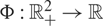 $\Phi :\mathbb{R}_ + ^2 \to {\mathbb{R}}$ such that Φ(t, ⋅) ∈ L 2(𝒯) for any t ∈ 𝒯, the corresponding RKHS is defined as
 $${{\cal H}_\Phi }{\kern 1pt} : = {\kern 1pt} \{ \int_0^t \Phi (t,s){\kern 1pt} f(s){\kern 1pt} {\rm {d}}s,t \in {\cal T}{\kern 1pt} :{\kern 1pt} f \in {{\rm {L}}^2}({\cal T})\} ,$$
with inner product
 $${\langle \int_0^ \cdot \Phi ( \cdot ,s){\kern 1pt} {f_1}(s){\kern 1pt} ds,\int_0^ \cdot \Phi ( \cdot ,s){\kern 1pt} {f_2}(s){\kern 1pt} {\rm {d}}s\rangle _{{{\cal H}_\Phi }}}{\kern 1pt} : = {\kern 1pt} {\langle {\kern 1pt} {f_1},{f_2}\rangle _{{{\rm {L}}^2}({\cal T})}}.$$
Reproducing kernel Hilbert spaces, together with their inner products, turn out to provide the right spaces to characterise large deviations rate functions. In particular, for a given Gaussian Volterra process of the form 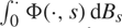 $\int_0^ \cdot \Phi ( \cdot ,s){\kern 1pt} {\rm {d}}{B_s}$, for some Volterra kernel Φ, it follows from [Reference Deuschel and Stroock19, Theorem 3.4.5] that the sequence
 ${(\varepsilon \int_0^ \cdot \Phi ( \cdot ,s){\rm{d}}{B_s})_{\varepsilon > 0}}$ satisfies a large deviations principle with speed ε 2 and rate function
 $${\Lambda _\Phi }(\varphi ) = \left\{ {\matrix{
{{1 \over 2}\parallel \dot \varphi {\parallel _{{{\cal H}_\Phi }}},} \hfill & {{\rm{if}}\varphi \in {{\cal H}_\Phi },} \hfill \cr
{ + \infty ,} \hfill & {{\rm{otherwise}}.} \hfill \cr
} } \right.$$
An obviously special role is played by the standard Brownian motion  $H = {1 \over 2}$, and we shall adopt the simplified notation ℋ (the classical Cameron–Martin space) and Λ in place of ℋK 1/2 and ΛK1/2.
2.2. Setting and assumptions
The particular system we are interested in is
 $${\rm {d}}{X_t} = - {\textstyle{1 \over 2}}\sigma {({Y_t})^2}{\rm {d}}t + \sigma ({Y_t})(\rho {\rm {d}}{B_t} + \overline \rho dB_t^ \bot ),\quad \quad{X_0} = 0,$$
 $${\rm {d}}{Y_t} = (\lambda + \beta {Y_t}){\rm {d}}t + \xi {\rm {d}}W_t^H,\quad \quad{Y_0} \sim \Theta ,$$
where WH is a fractional Brownian motion with Hurst parameter H ∈ (0, 1), (B, B ⊥) is a two-dimensional standard Brownian motion, β < 0, λ, ξ > 0, ρ ∈ (−1, 1), 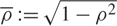 $\overline \rho {\kern 1pt} : = {\kern 1pt} \sqrt {1 - {\rho ^2}} $, and Θ is a square-integrable continuous random variable. In order to guarantee the existence and uniqueness of a strong solution, we further assume [Reference Mishura44, Theorem 3.1.3] that σ is Lipschitz continuous, satisfies the growth condition |σ(y)| ≤ C(1 + |y|) for y ∈ ℝ, and is differentiable with a locally Hölder-continuous derivative. In order to prove our main results below, we make the following technical assumption.
Assumption 𝒜. There exists a measurable function  $\widetilde\sigma :\mathbb {R} \to \mathbb{R} $, with locally Hölder-continuous derivative, such that the scaling property
 $\mathop {\lim }\nolimits_{\varepsilon \downarrow 0} \varepsilon \sigma (y/\varepsilon ) = \widetilde\sigma (y)$ holds true uniformly on ℝ.
Remark 2.1. Since the map σ is Lipschitz continuous with linear growth, then so is  $\widetilde\sigma $. The scaling property further implies that
 $\mathop {\lim }\nolimits_{\varepsilon \downarrow 0} {\varepsilon ^b}\sigma (y/{\varepsilon ^b}) = \widetilde\sigma (y)$ uniformly on ℝ for any b > 0. This will be useful for later computations.
3. Main results
The centrepiece of our analysis are large deviations estimates for suitably rescaled versions of (2.5). The first rescaling (presented in Section 3.1) is tailored to the analysis of the tail behaviour of (2.5), while the second rescaling (Section 3.2) is bespoke to its short-time asymptotic properties. In addition to these asymptotic results in the general fractional case (Theorems 3.1 and 3.4), we present two special simplified diffusive cases, where particularly tractable rate functions can be obtained (Theorems 3.3 and 3.6 respectively). For this we impose stronger conditions (Assumption 3.1) on the random starting point. This allows us to establish, following [Reference Millet, Nualart and Sanz43] in Section 3.1.2, an exponential equivalence between (2.5) and an analogous process with fixed starting point. In Section 3.2.2 we construct a third rescaling (3.8) inspired by Mellouk [Reference Mellouk42] in the short-time diffusive case under the assumption that the support of the random starting point is bounded. We shall work with rescaled versions Yε of the process Y in (2.5) (see (3.1) and (3.6) for specific examples), together with a function hε describing the speed of the large deviations estimates, for which we introduce the following assumptions.
Assumption 𝒜. There is a family of continuous functions (σn)n≥0 on ℝ such that
(i) (σn)n≥0 converges uniformly to
 $\widetilde\sigma $ on ℝ;
(ii) for all δ > 0,
$\mathop {\lim }\nolimits_{n \uparrow \infty } \mathop {\limsup }\nolimits_{\varepsilon \downarrow 0} {h_\varepsilon }\log {\kern 1pt} \;{\rm {P}}{\kern 1pt} (|{\sigma _n}({Y^\varepsilon }) - \widetilde\sigma ({Y^\varepsilon }) \ge \delta |) = - \infty $.


Assumption  ${\cal A}_b^\Theta $. (Tail behaviour of Θ.) lim supε↓0 hε log P(εb|Θ| > 1) = −∞.
In Assumptions 𝒜 ′ and  ${\cal A}_b^\Theta $ above, the large deviations speed hε takes the value ε 2b in Section 3.1 and ε 4H+2b in Section 3.2 respectively. The constant b (which may vary below) plays an essential role in subsequent large deviations estimates, via exponential equivalence techniques (Definition 2.3). Assumptions 𝒜 and 𝒜 ′ are naturally satisfied in the fractional Stein–Stein case (where σ (y) ≡ y), but imposing them allows us to state our results for more general σ, in particular when using extended contraction principles [Reference Mayer-Wolf, Nualart and PéRez-Abreu40, Proposition 2.3].
3.1. Tail behaviour
3.1.1 The general case
For b, ε > 0, introduce the rescaling (Xε, Yε) := (ε 2b X, εbY), so that (2.5) becomes
 $${\rm {d}}X_t^\varepsilon = - {{{\varepsilon ^{2b}}} \over 2}\sigma {({{Y_t^\varepsilon } \over {{\varepsilon ^b}}})^2}{\rm {d}}t + {\varepsilon ^{2b}}\sigma ({{Y_t^\varepsilon } \over {{\varepsilon ^b}}})(\rho {\rm {d}}{B_t} + \overline \rho dB_t^ \bot ),\quad \quad X_0^\varepsilon = 0,$$
 $${\rm {d}}Y_t^\varepsilon = ({\varepsilon ^b}\lambda + \beta Y_t^\varepsilon ){\kern 1pt} {\rm {d}}t + {\varepsilon ^b}\xi {\rm {d}}W_t^H,\quad \quad \quad Y_0^\varepsilon \sim {\varepsilon ^b}\Theta .$$
The particular rescaling considered here is perfectly suited for tail behaviour, as large deviations provide estimates for P(Xε ≥ 1) = P(X ≥ ε −2b). Our main result is as follows, and is proved in Appendix A.1.3:
Theorem 3.1. For any H ∈ (0, 1), the following hold:
(i) for any b > 0 such that
${\cal A}_b^\Theta $ holds, Yε ~ LDP(ε 2b, ΛFH), with Λ FH in (2.4) and FH in Lemma 3.1;(ii) for any
$b \ge {1 \over 2}$ such that 𝒜, 𝒜 ′, ${\cal A}_b^\Theta $ hold, ${X^\varepsilon } \sim LDP({\varepsilon ^{2b}},\widetilde\Lambda )$, with $\widetilde\Lambda $ in (A.2).




The proof of the theorem, developed later, requires a precise analysis of the RKHS of the processes under consideration, and we first state two key ingredients (proved in Appendices A.1.1 and A.1.2), which are also of independent interest. Recall from [Reference Yan, Lu and Xu53, Definition 2.1] the definition of the stochastic integral: for any smooth function f on 𝒯 with bounded derivatives such that  $\parallel f\parallel {\kern 1pt} : = {\kern 1pt} \int_{\cal T} {(\Gamma _{H,\,t}^*{\kern 1pt} f(t))^2}{\kern 1pt} {\rm {d}}t \lt \infty $, define, for t ∈ 𝒯,
 $\int_0^t {\kern 1pt} f(u){\kern 1pt} {\rm {d}}W_u^H{\kern 1pt} : = {\kern 1pt} \int_0^t \Gamma _{H,\,t}^*{\kern 1pt} f(u){\kern 1pt} {\rm {d}}{Z_u}$, with
 $$\Gamma _{H,t}^*{\kern 1pt} f(s){\kern 1pt} : = {\kern 1pt} - {{{\kappa _H}} \over {{s^{{H_ - }}}}}{{\rm {d}} \over {{\rm {d}}s}}\int_s^t {u^{{H_ - }}}{(u - s)^{{H_ - }}}f(u){\kern 1pt} {\rm {d}}u,\quad \quad {\rm{forall}}s \in (0,t].$$
Lemma 3.1. For H ∈ (0, 1) and β > 0, there exists a Brownian motion Z such that
 $$\xi \int_0^t {e^{\beta (t - s)}}{\kern 1pt} {\kern 1pt} \;{\rm {d}}{\kern 1pt} W_s^H = \int_0^t {F^H}(t,s){\kern 1pt} {\kern 1pt} \;{\rm {d}}{\kern 1pt} {Z_s}$$
holds almost surely for t ∈ 𝕋, where FH : 𝒯 × 𝒯 → ℝ is defined for 0 < s < t, with κH in (2.2), as
 $${F^H}(t,s){\kern 1pt} : = {\kern 1pt} \left\{ {\matrix{
{{{\xi {\kappa _H}} \over {{s^{{H_ - }}}}}[[t(t - s{{)]}^{{H_ - }}}} \hfill & {} \hfill \cr
{\quad \quad \quad \quad + \int_s^t \{ {{1 - 2H} \over {2u}} + \beta \} [u(u - s{{)]}^{{H_ - }}}{e^{\beta (t - u)}}{\kern 1pt} du],} \hfill & {{\rm{if}}H \lt {1 \over 2},} \hfill \cr
{{{\xi {\kappa _H}{H_ - }} \over {{s^{{H_ - }}}}}\int_s^t {{{u^{{H_ - }}}{e^{\beta (t - u)}}} \over {{{(u - s)}^{1 - {H_ - }}}}}{\kern 1pt} du,} \hfill & {{\rm{if}}H > {1 \over 2},} \hfill \cr
{\xi {e^{\beta (t - s)}},} \hfill & {{\rm{if}}H = {1 \over 2}.} \hfill \cr
} } \right.$$
The case β = 0 (and ξ = 1) is excluded since, in that case, the lemma boils down to the classical Volterra representation of the fractional Brownian motion (2.1) and the function FH is just the kernel KH given in (2.2). For  $H \in ({1 \over 2},1)$, the expression for FH is in agreement with [Reference Yan, Lu and Xu53, Definition 2.1], but for
 $H \in (0,{1 \over 2})$ it corrects the slightly erroneous expression therein. This function FH allows us to fully characterise the following RKHS, with proof postponed to Section A.1.2:
Proposition 3.1. For any H ∈ (0, 1), β > 0, the space ℍ FH is the RKHS of the Gaussian process  $\xi \int_0^ \cdot {e^{\beta ( \cdot - s)}}{\kern 1pt} {\kern 1pt} \;d{\kern 1pt} W_s^H$.
3.1.2 The Millet–Nualart–Sanz approach
In [Reference Millet, Nualart and Sanz43], Millet, Nualart, and Sanz considered a perturbed stochastic differential equation of the form
 $$dX_t^\varepsilon = {\rm b} (\varepsilon ,X_t^\varepsilon ){\rm {d}}t + \varepsilon (X_t^\varepsilon )d{W_t}.$$
Here, for any ε > 0, the functions 𝔟(ε, ⋅): ℝn → ℝn and 𝔞 : ℝn → ℳ (n, d)(ℝ) are bounded Borel measurable and uniformly Lipschitz, 𝔟(ε, ⋅) converges uniformly to a function 𝔟(⋅) as ε tends to zero, W is a d-dimensional Brownian motion, and  $X_0^\varepsilon $ is an ℝn-valued square-integrable random variable. Proofs of the existence and uniqueness of a strong solution can be found in [Reference Friedman24, Chapter 5, Theorem 2.1]. Following classical large deviations steps, consider, for any φ ∈ ℋ, the following controlled ordinary differential equation (ODE) on 𝒯 :
 $${\dot \psi _t} = {\rm a}({g_t}){\dot \varphi _t} + {\rm b}({\psi _t}),$$
the solution flow of which, starting from x0 ∈ ℝn, is denoted by  ${{\cal S}_{{x_0}}}(\varphi )$. Millet, Nualart, and Sanz [Reference Millet, Nualart and Sanz43] proved a large deviations principle [Reference Millet, Nualart and Sanz43, Theorem 4.1] for the sequence (Xε)ε>0 under the following assumption.
Assumption 3.1. Both 𝔞(⋅) and 𝔟(⋅) belong to  ${\cal C}_b^2$, and there exists x 0 ∈ ℝn such that, for any δ > 0,
 $$\mathop {\limsup }\limits_{\varepsilon \downarrow 0} {\varepsilon ^2}\log {\kern 1pt} \;{\rm {P}}{\kern 1pt} (|X_0^\varepsilon - {x_0}| > \delta ) = - \infty .$$
Theorem 3.2. Under Assumption 3.1, (Xε)ε>0 ~ LDP(ε 2, I) with  $I(\psi ) = \inf \{ \Lambda (\varphi ){\kern 1pt} :{\kern 1pt} \varphi \in {\cal H},\psi = {{\cal S}_{{x_0}}}(\varphi )\} $.
Condition (3.4) is an exponential equivalence property between the initial random variable  $X_0^\varepsilon $ and the constant x0, and ensures that large deviations are preserved under exponentially small perturbations of the starting point. Therefore, in the standard diffusion case
 $H = {1 \over 2}$, it is possible to obtain a similar result to Theorem 3.1 with a simplified rate function (albeit with stronger restrictions on the starting point) by using the approach in [Reference Millet, Nualart and Sanz43]. For this, we rewrite (3.3) to correspond to (3.1), albeit with stronger assumptions on the coefficients, with W := (W 1, W 2)′ a Brownian motion, Xε = (Xε, Yε),
 $H = {1 \over 2}$, ε → εb,
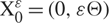 $X_0^\varepsilon = (0,\varepsilon \Theta )$, and
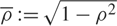 $\overline \rho {\kern 1pt} : = {\kern 1pt} \sqrt {1 - {\rho ^2}} $:
 $${\rm{b}}(\varepsilon ,X_t^\varepsilon ) = \left( {\matrix{
{ - {1 \over 2}\widetilde\sigma {{(Y_t^\varepsilon )}^2}} \cr
{\varepsilon \lambda + \beta Y_t^\varepsilon } \cr
} } \right)\quad \quad {\rm{and}}\quad \quad {\rm{a}}(X_t^\varepsilon ) = \left( {\matrix{
{\overline \rho \widetilde\sigma (Y_t^\varepsilon )} & {\rho \widetilde\sigma (Y_t^\varepsilon )} \cr
0 & \xi \cr
} } \right).$$
The correlation between the two components of W is explicitly represented in the diffusion matrix 𝔞.
Theorem 3.3. Under Assumption 3.1, the solution Xε to (3.3) satisfies (Xε)ε>0 ~ LDP(ε 2, I) with  ${\bf{I}}(\chi ) = \inf \{ \Lambda (\varphi ){\kern 1pt} :{\kern 1pt} \varphi \in {\cal H},\chi = {{\cal S}_{{x_0}}}({\Psi ^\rho }(\varphi ))\} $ and
 $${\Psi ^\rho }{\kern 1pt} :{\mathbb {R}} {^2}z \mapsto \left( {\matrix{
{\overline \rho } & \rho \cr
0 & 1 \cr
} } \right)z,.$$
Proof. The proof of Theorem 3.2 relies first on proving a large deviations principle for the flow  ${{\cal S}_{{x_0}}}$ using Schilder’s Theorem [Reference Dembo and Zeitouni16, Theorem 5.2.3], then on extending this LDP to the original system. One can easily extend it to include a correlation parameter ρ ∈ (−1, 1), the main difference being the rate function. Indeed, since
 $W_2^ \bot $ and W 2 are independent, Schilder’s Theorem yields that
 $\varepsilon (W_2^ \bot ,{W_2})' \sim {\rm LDP}({\varepsilon ^2},\Lambda )$. Since the map Ψρ is continuous on (𝒞, ||⋅||∞) and
 $\varepsilon W' = {\Psi ^\rho }(\varepsilon (W_2^ \bot ,{W_2})')$, the theorem follows from the contraction principle giving an LDP for εW′ as ε tends to zero with speed ε 2 and good rate function
 $${\Lambda ^\rho }(\psi ){\kern 1pt} : = {\kern 1pt} \inf \{ \Lambda (\varphi ){\kern 1pt} :{\kern 1pt} \varphi \in {\cal H},\psi = {\Psi ^\rho }(\varphi )\} .$$
This completes the proof.
3.2. Small-time behaviour
We now tackle the small-time behaviour of the process (2.5). Under the general set of assumptions 𝒜, 𝒜 ′,  ${\cal A}_b^\Theta $, we need to introduce a particular rescaling both in time and in space in order to observe some weak convergence. This is different from the classical Itô diffusion case (with fixed starting point), where solutions of such SDEs generally converge in small time. In the Itô case, though, if the distribution of the starting point has compact support, we show in Section 3.2.2 that space rescaling is not required any longer.
3.2.1 The general case
The rescaling  $(X_t^\varepsilon ,Y_t^\varepsilon ){\kern 1pt} : = {\kern 1pt} ({\varepsilon ^{2H + 2b - 1}}{X_{{\varepsilon ^2}t}},{\varepsilon ^b}{Y_{{\varepsilon ^2}t}})$, for b > 0, turns (2.5) into
 $$dX_t^\varepsilon = - {{{\varepsilon ^{2H + 1 + 2b}}} \over 2}\sigma {({{Y_t^\varepsilon } \over {{\varepsilon ^b}}})^2}{\rm {d}}t + {\varepsilon ^{2H + 2b}}\sigma ({{Y_t^\varepsilon } \over {{\varepsilon ^b}}})(\rho {\rm {d}}{B_t} + \overline \rho {\rm {d}}B_t^ \bot ),\,\,\,\,\,X_0^\varepsilon = 0,$$
 $$dY_t^\varepsilon = ({\varepsilon ^{b + 2}}\lambda + \beta {\varepsilon ^2}Y_t^\varepsilon ){\rm {d}}t + {\varepsilon ^{2H + b}}\xi {\rm {d}}W_t^H,\,\,\,\,\,\,\,\,\,\,Y_0^\varepsilon \sim {\varepsilon ^b}\Theta .$$
Our main result is as follows:
Theorem 3.4. For any H ∈ (0, 1),
(i) for any b > 0 such that
${\cal A}_b^\Theta $ holds, ${Y^\varepsilon } \sim LDP({\varepsilon ^{4H + 2b}},{\Lambda _{G_0^H}})$, with ${\Lambda _{G_0^H}}$ in (2.4);(ii) if
$b \ge {1 \over 2} - 2H$ such that 𝒜, 𝒜 ′, ${\cal A}_b^\Theta $ hold, Xε ~ LDP(ε 4H+2b, I), with I in (A.5).




The proof of (i) is similar to that of Theorem 3.1(i) and relies on proving LDP for an auxiliary process, defined in (A.1), exponentially equivalent to the original (rescaled) process Yε. The proof of (ii) is more involved and is postponed to Appendix A.2.
In order to state the following key result, define, for any ε > 0,  $G_\varepsilon ^H$ as the function FH in Lemma 3.1, replacing β by βε 2, and for s, t ∈ 𝒯 with 0 < s < t, its pointwise limit
 $$\matrix{
{G_0^H(t,s){\kern 1pt} : = {\kern 1pt} \mathop {\lim }\limits_{\varepsilon \downarrow 0} G_\varepsilon ^H(t,s)} \hfill \cr
{ = \left\{ {\matrix{
{{{\xi {\kappa _H}{H_ - }} \over {{s^{{H_ - }}}}}\int_s^t {{{u^{{H_ - }}}} \over {{{(u - s)}^{1 - {H_ - }}}}}{\kern 1pt} {\rm {d}}u,} \hfill & {{\rm{for}}H \in ({1 \over 2},1),} \hfill \cr
{{{\xi {\kappa _H}} \over {{s^{{H_ - }}}}}((t(t - s{{))}^{{H_ - }}} - {H_ - }\int_s^t {{(u - s)}^{{H_ - }}}{u^{{H_ - } - 1}}{\kern 1pt} {\rm {d}}u),} \hfill & {{\rm{for}}H \in (0,{1 \over 2}),} \hfill \cr
{\xi ,} \hfill & {{\rm{for}}H = {1 \over 2}.} \hfill \cr
} } \right.} \hfill \cr
} $$
The following proposition is similar to Proposition 3.1, as  $G_0^H(t, \cdot ) \in {{\rm {L}}^2}({\cal T})$ and, for all 0 < s < t,
 $G_0^H(t,s) > 0$, and its proof is omitted.
Proposition 3.2. For any H ∈ (0, 1), the space  ${{\cal H}_{G_0^H}}$ is the RKHS of the Gaussian process
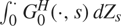 $\int_0^ \cdot G_0^H( \cdot ,s){\kern 1pt} d{Z_s}$
3.2.2. Small-time asymptotics for bounded support in the diffusion case
In the standard case  $H = {1 \over 2}$, the rescaling in the previous subsection is not really ‘natural’, in the sense that small- time weak convergence usually holds for Itô diffusions without space rescaling. In this case, using an approach introduced by Bezuidenhout [Reference Bezuidenhout10] and further developed by Mellouk [Reference Mellouk42], we can obtain simpler large deviations estimates if the support of the initial datum is bounded. A simplified version of Mellouk considers, for any ε > 0, the following system on 𝒯:
 $${\rm {dX}}_t^\varepsilon = {\rm {b}}({\rm {X}}_t^\varepsilon,\,{\rm {Z}}){\rm {d}}t + \varepsilon {\rm {a}}({\rm {X}}_t^\varepsilon,\,{\rm {Z}}){\rm {d}}{{\rm {W}}_t},\quad \quad {\rm {X}}_0^\varepsilon = {{\rm {x}}_0} \in {\mathbb {R}}{^n},$$
where 𝔟 : ℝn × ℝm → ℝn and 𝔞 : ℝn × ℝm → ℳ (n, d) are bounded Borel measurable, uniformly Lipschitz continuous, Z is a random variable with compact support on ℝm, and W is a d-dimensional standard Brownian motion, independent of Z. The main result of the paper is a large deviations principle on 𝒞α(𝒯, ℝn), the space of α-Hölder continuous functions, for  $0 \le \alpha \lt {1 \over 2}$, for the sequence (Xε)ε>0 under the following assumptions.
(H1) 𝔟(⋅, ⋅) is jointly measurable on ℝn × ℝm and there exists C > 0 such that, for all x, x ′ ∈ ℝn, z, z ′ ∈ ℝm,
$$|{\rm {b}}(x,z)| \le C(1 + |x|)\quad \quad and\quad \quad |{\rm {b}}(x,z) - {\rm {b}}(x',z')| \le C(|x - x| + |z - z'|).$$
(H2) 𝔞(⋅, ⋅) is jointly measurable on ℝn × ℝm and there exists C > 0 such that, for all x, x ′ ∈ ℝn, z, z ′ ∈ ℝm,
$$\parallel {\rm {a}}(x,z)\parallel \le C\quad \quad and\quad \quad \parallel {\rm {a}}(x,z) - {\rm {a}}(x',z')\parallel {\rm {a}}\le C(|x - x'| + |z - z'|).$$


For f ∈ ℋ, u ∈ supp(Z) and x0 ∈ ℝn, let  ${{\cal S}_{{x_0}}}(f,u)$ denote the unique solution to the controlled ODE
 ${g_t} = {x_0} + \int_0^t {\rm {b}}({g_s},{u_s}){\kern 1pt} {\rm {d}}s + \int_0^t {\rm {a}}({g_s},{u_s}){\kern 1pt} {\dot f_s}{\kern 1pt} {\rm {d}}s$, for t ∈ 𝒯. Let us now introduce the following definition:
Definition 3.1. Let  $\alpha \in [0,{1 \over 2})$ and ℬa be the ball of radius a in the α-Hölder norm. The lower semi-continuous regularisation Ĭ : 𝒞α(𝒯, ℝm) → 𝒞α(𝒯, ℝm) of a functional I : 𝒞α(𝒯, ℝm) → 𝒞α(𝒯, ℝm) is defined as
 $$\mathord{\buildrel{\lower3pt\hbox{$\scriptscriptstyle\smile$}}\over
I} (\psi ): = \mathop {\lim }\limits_{a \downarrow 0} \inf \{ I(\varphi ):\varphi \in {B_a}(\psi )\} .$$
Theorem 3.5. (Theorem 2.1 in [Reference Mellouk42].) Under Assumption 3.2, (Xε)ε>0 ~ LDP(ε 2, Ĭα), where, with Λ in (2.4),
 $${I^\alpha }(\psi ){\kern 1pt} : = {\kern 1pt} \inf \{ \Lambda (\varphi ){\kern 1pt} :{\kern 1pt} \varphi \in {\cal H},{{\cal S}_{{x_0}}}(\varphi ,u) = \psi ,for\,some\,u \in supp(Z)\} .$$
Coming back to our model, the rescaling  $ (X_t^\varepsilon ,Y_t^\varepsilon ){\kern 1pt} : = {\kern 1pt} ({X_{{\varepsilon ^2}t}},{Y_{{\varepsilon ^2}t}}) $, equivalent to that of Section 3.2.1 with b = 0 and
 $H = {1 \over 2}$, the small-noise system (2.5), under Assumption 𝒜, becomes, similarly to Section 3.2.1,
 $${\rm {d}}X_t^\varepsilon = - {{{\varepsilon ^2}} \over 2}\widetilde\sigma {(Y_t^\varepsilon )^2}{\rm {d}}t + \varepsilon \widetilde\sigma (Y_t^\varepsilon )(\rho {\rm {d}}{B_t} + \overline \rho {\rm {d}}B_t^ \bot ),\quad {X_0^\varepsilon} = 0,$$
 $${\rm {d}}Y_t^\varepsilon = ({\varepsilon ^2}\lambda + \beta {\varepsilon ^2}Y_t^\varepsilon ){\kern 1pt} {\rm {d}}t + \varepsilon \xi {\rm {d}}{B_t},\quad \quad {Y_0^\varepsilon} \sim \Theta ,$$
with B a standard Brownian motion. Subtracting the initial random datum  $X_0^\varepsilon = {X_0} = (0,\Theta )'$, this system can be expressed in the form (3.7) with Xε = (Xε, Yε),
 $$b(\varepsilon ,{{\rm{X}}^\varepsilon },{{\rm{X}}_0}) = {\varepsilon ^2}\left( {\matrix{
{ - {1 \over 2}\sigma {{(Y_t^\varepsilon + \Theta )}^2}} \cr
{\lambda + \beta (Y_t^\varepsilon + \Theta ){\rm{ }}} \cr
} } \right),{\rm{and}}\,a({{\rm{X}}^\varepsilon },{{\rm{X}}_0}) = \left( {\matrix{
{\rho \sigma (Y_t^\varepsilon + \Theta )} & {\bar \rho \tilde \sigma (Y_t^\varepsilon + \Theta )} \cr
\xi & 0 \cr
} } \right),$$
and note that 𝔟(ε, ⋅, ⋅) converges to the null map as ε tends to zero. The assumptions imposed in [Reference Mellouk42] on the drift and diffusion coefficients are clearly satisfied here. While Mellouk allows the drift and diffusion to depend explicitly on external random factors, we can write our setting (dependence on a random starting point) into this framework. The large deviations estimate for the sequence (Xε)ε>0 = (Xε, Yε)ε>0 thus obtained is stronger than that in the previous section, as it holds on 𝒞α(𝒯, ℝn), for any  $0 \le \alpha \lt {1 \over 2}$. Note that the mild conditions on the coefficients [Reference Mellouk42, (H 0)–(H 2)] are easily satisfied in our case, so the only additional assumption is the boundedness of the support on Θ. We remark here that [Reference Mellouk42] is not directly applicable to the current setting but has to be extended to include ε-dependence in the drift, and we do so following the approach developed by Peithmann [Reference Peithmann47, Section 2.2.1] as inspired by Azencott [Reference Azencott4]. In order to state LDP (proved in Section A.3), we impose the following assumption.
Assumption 3.3. For u ∈ supp(X 0) and φ ∈ ℋ, the ODE  ${\psi _t} = \int_0^t a({\psi _s},{u_s}){\dot \varphi _s}{\kern 1pt} ds$ has a unique solution on 𝒯, denoted by 𝒮 0(φ, u).
Theorem 3.6. Under Assumption 3.3, if Θ has compact support then (Xε)ε>0 ~ LDP(ε 2, Ĭα), with Λρ defined in (3.5) and
 $${I^\alpha }(\psi ){\kern 1pt} : = {\kern 1pt} \inf \{ {\Lambda ^\rho }(\varphi ){\kern 1pt} :{\kern 1pt} \varphi \in {\cal H},\,such\,that\, {{\cal S}_0}(\varphi ,u) = \psi,\,for\,some\, u \in supp({X_0})\} .$$
4. Applications to implied volatility asymptotics
As announced in the introduction, we unify two branches of research here, both aimed at reproducing the steepness of the implied volatility surface on the short end via models with continuous paths. While there are now numerous outputs [Reference Alô’s, Leòn and Vives3, Reference Bayer, Friz and Gatheral7, Reference Bayer8, Reference Forde and Zhang23, Reference Fukasawa26, Reference Gatheral, Jaisson and Rosenbaum30, Reference Jacquier, Pakkanen and Stone36] in the literature confirming that a fractional driving noise (with Hurst exponent H < 1/2) in the volatility leads to the observed steepness of the smile, recent results [Reference Jacquier and Roome37, Reference Jacquier and Shi39] reproduce this effect by randomising the initial volatility in classical diffusive models. In this section we demonstrate how to modulate the two effects with respect to one another. In the Black– Scholes–Merton model, the price of a European Call option is 𝒞 BS(t, ek, Σ), with associated volatility Σ. Considering a market with observed Call option prices 𝒞 obs(t, ek), with maturity t and strike ek, we denote by Σt(k) the implied volatility, defined as the unique non-negative solution to 𝒞 BS(t, ek, Σt(k)) = 𝒞 obs(t, ek).
4.1. General fractional case
From Theorems 3.1 and 3.4, we can deduce the asymptotic behaviour of the implied volatility for large strikes and for small maturities. We state those below, and postpone the proofs to Appendices A.4 and A.5.
Corollary 4.1. (Large-strike implied volatility asymptotics.) For any H ∈ (0, 1) and any b ≥ 1/2 such that Theorem 3.1 holds, we have the following large-strike asymptotic estimates of the implied volatility:
 $$\mathop {\lim }\limits_{k \uparrow \infty } {{\Sigma _t^2(k)t} \over k} = {1 \over 2}{(\mathop {\inf }\limits_{y \ge 1} \widetilde\Lambda (\phi {)|_{{\phi _t} = y}})^{ - 1}},\quad with\,{\rm{ }}\widetilde\Lambda {\rm{ }}\,as\,in{\rm{ (A}}{\rm{.2)}},and\,for\,any t\,\in {\cal T}.$$
Similarly, Theorem 3.4 yields the small-time behaviour of the implied volatility. The following corollary generalises [Reference Forde and Zhang23, Corollary 4.10].
Corollary 4.2. (Small-time implied volatility asymptotics.) For H ∈ (0, 1),  $b \ge {1 \over 2} - 2H$ such that Theorem 3.4 holds, the following small-time estimate is true for any k ≠ 0:
 $$\mathop {\lim }\limits_{t \downarrow 0} {t^b}\Sigma _t^2({t^{1/2 - H - b}}k) = {{{k^2}} \over 2}{(\mathop {\inf }\limits_{y \ge k} I(\phi {)|_{{\phi _1} = y}})^{ - 1}},\quad with\,I\,as\,in\,(26).$$
This implies that the implied volatility explodes with rate t −b. For b = 0, it is identical to [Reference Forde and Zhang23, Formula (26)].
4.2. Refined asymptotic results in the special diffusive case from Sections 3.1.2 and 3.2.2
4.2.1 Large-strike asymptotics
We consider here a specific case of a multidimensional diffusion, as we are only interested in studying its tail asymptotics. Let Xζ := (X ζ,1, ..., X ζ, n) be the unique strong solution in ℝn to
 $${\rm{dX}}_t^\zeta = \tilde b({\rm{X}}_t^\zeta ){\rm{d}}t + a({\rm{X}}_t^\zeta ){\rm{d}}{W_t},\quad \quad {\rm{X}}_0^\zeta = \zeta ,$$
for some d-dimensional standard Brownian motion and some square-integrable random variable ζ, and with 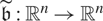 $\tilde{b} :{\mathbb R}^{n} \to {\mathbb R}^{n}$ and 𝔞 : ℝn → ℳ (n, d)(ℝ). Consider the following scaling assumption.
Assumption 4.1. There exist b 1, ..., bn > 0 with b 1 = 2 such that Xε,ζ := (ε b 1 X ζ,1, ..., ε b n Xζ,n) satisfies
 $${\rm{dX}}_t^{\varepsilon ,\zeta } = \varepsilon {\rm{\tilde b}}(\varepsilon ,{\rm{X}}_t^{\varepsilon ,\zeta })\;{\rm{d}}t + \varepsilon a({\rm{X}}_t^{\varepsilon ,\zeta }){\rm{d}}{W_t},\quad \quad {\rm{X}}_0^\zeta = ({\varepsilon ^{{b_1}}}{\zeta ^{(1)}}, \ldots ,{\varepsilon ^{{b_n}}}{\zeta ^{(n)}}).$$
Furthermore,  $\varepsilon \tilde{b}(\varepsilon , \cdot /\varepsilon )$ converges uniformly to some function 𝔟(⋅) as ε tends to zero.
We can then state the main result about tail asymptotics:
Proposition 4.1. Under Assumption 4.1, if there exists x0 ∈ ℝn for which any δ > 0 implies lim supε↓0 ε 2 log P(|ζ − x0| >δ) = −∞, and if the triple (x0, 𝔟(⋅), 𝔞(⋅)) satisfies Assumption 3.1, then
 $$\mathop {\lim }\limits_{\varepsilon \downarrow 0} {\varepsilon ^2}\log {\kern 1pt} \;{\rm {P}}{\kern 1pt} (\varepsilon X_t^{\zeta ,1} \ge 1) = \mathop {\lim }\limits_{\varepsilon \downarrow 0} {\varepsilon ^2}\log {\kern 1pt} \;{\rm {P}}{\kern 1pt} (\varepsilon X_t^{{x_0},1} \ge 1),\quad \quad for\,any\,t\,\in {\cal T}.$$
The scaling from Assumption 4.1 may be odd at first, but reflects the fact that components of stochastic models may each act on different scales. Consider, for example, the Ornstein– Uhlenbeck process, solution to
 $$\matrix{
\hfill {{\rm {d}}{X_t}} & \hfill { = - {1 \over 2}Y_t^2{\rm {d}}t + {Y_t}{\rm {d}}{W_t},} & \hfill {{X_0} = \zeta ,} \cr
\hfill {{\rm {d}}{Y_t}} & \hfill { = (\lambda + \beta {Y_t}){\rm {d}}t + \xi {\rm {d}}{B_t},} & \hfill {{Y_0} = {y_0} > 0,} \cr
} $$
where W and B are correlated Brownian motions. The rescaling (Xε, Yε) := (ε 2X, εY) (corresponding to b 1 = 2 and b 2 = 1) yields
 $$\matrix{
\hfill {{\rm {d}}X_t^\varepsilon } & \hfill { = - {1 \over 2}{{(Y_t^\varepsilon )}^2}{\rm {d}}t + \varepsilon Y_t^\varepsilon {\rm {d}}{W_t},} & \hfill {X_0^\varepsilon = {\varepsilon ^2}\zeta ,} \cr
\hfill {{\rm {d}}Y_t^\varepsilon } & \hfill { = (\varepsilon \lambda + \beta Y_t^\varepsilon ){\rm {d}}t + \varepsilon \xi {\rm {d}}{B_t},} & \hfill {Y_0^\varepsilon = \varepsilon {y_0} > 0,} \cr
} $$
namely (4.1), and the assumptions are satisfied.
The proof of Proposition 4.1 is postponed to Appendix A.6. The assumption of the random initial condition  $X_0^\zeta = \zeta $ being an ℱ 0-measurable distribution can be relaxed. Indeed, ℱ is the filtration generated by the Brownian motion W. Instead, one could work with a filtration
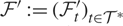 ${\cal F}'{\kern 1pt} : = {\kern 1pt} {({\cal F}{'_t})_{t \in {{\cal T}^*}}}$ generated by
 ${\cal F}{'_t}{\kern 1pt} : = {\kern 1pt} \sigma (\{ {W_u},u \le t\} \cup \{ \zeta \} )$, for all t ∈ 𝒯 *. Then the random initial point
 $X_0^\zeta $ has an ℱ ′0-measurable distribution and the results above still hold, in particular Theorem 3.2 and Proposition 4.1, on the new filtered probability space (Ω, ℱ ′, (ℱ ′)t∈T, P). In the context of implied volatility asymptotics, this result has the following meaning:
Corollary 4.3. The wings of the smile are independent of the starting point (ζ or x 0).
Proof. Gao and Lee [Reference Gao and Lee27] showed that the asymptotic behaviour of the implied volatility can be directly inferred from comparing tail probabilities to those of the Black–Scholes model. It is straightforward to see that the scaling of Proposition 4.1 is the same in Black–Scholes, and the corollary follows immediately.
4.2.2 Small-time asymptotics for the ‘forward’ Stein–Stein model
We are interested in a ‘forward’ process, as defined by Jacquier and Roome [Reference Jacquier and Roome37] in the context of forward-start European options:
 $${\mathbb {E}}{({{{S_{t + \tau }}} \over {{S_t}}} - {e^k})^ + } = E{({e^{{X_{t + \tau }} - {X_t}}} - {e^k})^ + }{\kern 1pt} = :{\kern 1pt} E{({e^{X_\tau ^{(t)}}} - {e^k})^ + },$$
with  ${(X_\tau ^{(t)})_{\tau \ge 0}}$ the so-called ‘forward’ process, defined path-wise by
 $X_\tau ^{(t)}{\kern 1pt} : = {\kern 1pt} {X_{t + \tau }} - {X_t}$, for some fixed t > 0 and for all τ ≥ 0. The ‘forward’ process
 ${(X_\tau ^{(t)})_{\tau \ge 0}}$ then satisfies the following stochastic differential equation:
 $$dX_\tau ^{(t)} = - {1 \over 2}{(Y_\tau ^{(t)})^2}d\tau + Y_\tau ^{(t)}d{W_{1,\tau }},X_0^{(t)} = 0,$$
 $$dY_\tau ^{(t)} = (\lambda + \beta Y_\tau ^{(t)})d\tau + \xi d{W_{2,\tau }},Y_0^{(t)} \sim {\sigma _t}.$$
The stochastic differential equation for 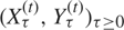 ${(X_\tau ^{(t)},Y_\tau ^{(t)})_{\tau \ge 0}}$ is the same as that for (Xt, Yt)t≥0, albeit with an initial random distribution (δ 0, σt), where σt is Gaussian with mean
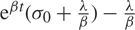 ${e^{\beta t}}({\sigma _0} + {\lambda \over \beta }) - {\lambda \over \beta }$ and variance
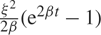 ${{{\xi ^2}} \over {2\beta }}({e^{2\beta t}} - 1)$. We now apply the results of Section 3.2.2 to obtain small-time asymptotics for a version of the Stein–Stein ‘forward’ model with a generalised random starting point.
Proposition 4.2. With the scaling  $(X_\tau ^\varepsilon ,Y_\tau ^\varepsilon ){\kern 1pt} : = {\kern 1pt} (X_{{\varepsilon ^2}\tau }^{(t)},Y_{{\varepsilon ^2}\tau }^{(t)})$ for ε, t > 0, the randomised Stein–Stein rescaled model (4.2) is the same as (3.8) with coefficients given in (3.9), with
 $\widetilde\sigma (y) \equiv y$, and Theorem 3.6 applies.
We can translate this result into forward implied volatility asymptotics directly using [Reference Forde and Jacquier21, Theorem 2.4], and refer to this very paper for a precise definition of the forward implied volatility Σt,τ :
Corollary 4.4. The small-time forward smile reads  $\mathop {\lim }\nolimits_{\tau \downarrow 0} \Sigma _{t,\tau }^2(k) = {{{k^2}} \over 2}{(\mathop {\inf }\nolimits_{y \ge k} {\kern 1pt} {\kern 1pt} {I^\alpha }(\phi {)|_{{\phi _1} = y}})^{ - 1}}$ with Ĭα in Theorem 3.6.
Appendix A. Proofs
A.1. Proof of Theorem 3.1
A.1.1. Proof of Lemma 3.1
From [Reference Yan, Lu and Xu53, Definition 2.1], for any smooth function f on 𝒯 with bounded derivatives such that  $\parallel f\parallel {\kern 1pt} : = {\kern 1pt} \int_{\cal T} {(\Gamma _{H,t}^*{\kern 1pt} f(t))^2}{\kern 1pt} dt \lt \infty $, define, for t ∈ 𝒯,
 $\int_0^t f(u){\kern 1pt} dW_u^H{\kern 1pt} : = {\kern 1pt} \int_0^t \Gamma _{H,t}^*{\kern 1pt} f(u){\kern 1pt} d{Z_u}$, with
 $$\Gamma _{H,t}^*{\kern 1pt} f(s){\kern 1pt} : = {\kern 1pt} - {{{\kappa _H}} \over {{s^{{H_ - }}}}}{d \over {ds}}\int_s^t {u^{{H_ - }}}{(u - s)^{{H_ - }}}f(u){\kern 1pt} du,\quad \quad for\,all\,s \in (0,t].$$
Introduce the function  ${\omega _s}(t){\kern 1pt} : = {\kern 1pt} {(t - s)^{{H_ - }}}{t^{{H_ - }}}$. Applying this to f(s) := ξeβ(t−s), one obtains the following:
(1) For
$H \lt {1 \over 2}$, using integration by parts and Leibniz’ integration rule,$$\matrix{
{{d \over {ds}}\int_s^t {u^{{H_ - }}}{{(u - s)}^{{H_ - }}}f(u){\kern 1pt} du} \hfill \cr
{ = {d \over {ds}}\{ {{\xi {{(t - s)}^{{H_ + }}}{t^{{H_ - }}}} \over {{H_ + }}}\} } \hfill \cr
{\quad + {d \over {ds}}\{ - \xi {{{H_ - }} \over {{H_ + }}}\int_s^t {{{{(u - s)}^{{H_ + }}}} \over {{u^{1 - {H_ - }}}}}{e^{\beta (t - u)}}{\kern 1pt} du + \xi {\beta \over {{H_ + }}}\int_s^t {{(u - s)}^{{H_ + }}}{u^{{H_ - }}}{e^{\beta (t - u)}}{\kern 1pt} du\} } \hfill \cr
{ = - \xi {{(t - s)}^{{H_ - }}}{t^{{H_ - }}} + \xi {H_ - }\int_s^t {{{\omega _s}(u)} \over u}{e^{\beta (t - u)}}{\kern 1pt} du - \xi \beta \int_s^t {\omega _s}(u){e^{\beta (t - u)}}{\kern 1pt} du.} \hfill \cr
} $$
Hence,
$$\matrix{
{\Gamma _{H,t}^*{\kern 1pt} f(s){\kern 1pt} : = {\kern 1pt} - {{{\kappa _H}} \over {{s^{{H_ - }}}}}{d \over {ds}}\int_s^t {\omega _s}(u){\kern 1pt} f(u){\kern 1pt} du} \hfill \cr
{ = {{\xi {\kappa _H}} \over {{s^{{H_ - }}}}}[{\omega _s}(t) + \beta \int_s^t {\omega _s}(u){e^{\beta (t - u)}}{\kern 1pt} du - {H_ - }\int_s^t {{{\omega _s}(u)} \over u}{e^{\beta (t - u)}}{\kern 1pt} du].} \hfill \cr
} $$
(2) For
$H > {1 \over 2}$, using Leibniz’ integration rule,$$\matrix{
{{d \over {ds}}\int_s^t {\omega _s}(u){\kern 1pt} f(u){\kern 1pt} du} \hfill & = \hfill & {\int_s^t \xi {d \over {ds}}{\omega _s}(u){e^{\beta (t - u)}}{\kern 1pt} du} \hfill \cr
{} \hfill & = \hfill & { - \xi {H_ - }\int_s^t {u^{{H_ - }}}{{(u - s)}^{{H_ - } - 1}}{e^{\beta (t - u)}}{\kern 1pt} du,} \hfill \cr
} $$
and hence
$$\matrix{
{\Gamma _{H,t}^*{\kern 1pt} f(s){\kern 1pt} {\kern 1pt} } \hfill & {: = } \hfill & { - {{{\kappa _H}} \over {{s^{{H_ - }}}}}{d \over {ds}}\int_s^t {\omega _s}(u){\kern 1pt} f(u){\kern 1pt} du} \hfill \cr
{} \hfill & {} \hfill & {{{\xi {\kappa _H}{H_ - }} \over {{s^{{H_ - }}}}}\int_s^t {u^{{H_ - }}}{{(u - s)}^{{H_ - } - 1}}{e^{\beta (t - u)}}{\kern 1pt} du.} \hfill \cr
} $$


A.1.2. Proof of Proposition 3.1
In order to prove that ℋ FH is the RKHS of the Gaussian process  $\xi \int_0^ \cdot {e^{\beta ( \cdot - s)}}{\kern 1pt} {\rm {d}}W_s^H$, one needs to show that the operator 𝕂FH is a bijection from L2(𝒯) to ℋ FH and that ℋ FH is dense in 𝒞.
The operator 𝕂FH acting on L2(𝒯) defined by  $ ({\mathbb {K}}{_{{F^H}}}f)(t){\kern 1pt} : = {\kern 1pt} \int_0^t {F^H}(t,s){\kern 1pt} f(s){\kern 1pt} ds$ satisfies 𝕂FH L2(𝒯) =: H FH and is surjective. It is also injective on ℋ F H : let f ∈ L2(𝒯) be a non-zero function such that (𝕂FHf) = 0 on 𝒯 *. Similar to [Reference Forde and Zhang23], there is an interval [t 1, t 2] ⊂ 𝒯 where f has constant sign. Using previous notation, FH is defined, for t ∈ 𝒯 * and s ∈ (0, t], as
 ${F^H}(t,s){\kern 1pt} : = {\kern 1pt} \xi \Gamma _{H,t}^*{e^{\beta (t - s)}}$. The function
 $g(s){\kern 1pt} : = {\kern 1pt} \xi \int_t^s {u^{{H_ - }}}{(u - s)^{{H_ - }}}{e^{\beta (t - u)}}{\kern 1pt} du$ is increasing, hence FH(t, ⋅) is a positive function on [0, t] and
 $\int_{{t_1}}^{{t_2}} {F^H}(t,s){\kern 1pt} f(s){\kern 1pt} ds > 0$, leading to a contradiction. Thus 𝕂FH is injective on ℋ FH, hence bijective from L2(𝒯) to ℋ FH. Since 𝕂FH is a linear operator, one can then define
 ${\langle {\mathbb {K}}{_{{F^H}}}{f_1},{\mathbb {K}}{_{{F^H}}}{f_2}\rangle _{{{\cal H}_{{F^H}}}}}{\kern 1pt} : = {\kern 1pt} {\langle {f_1},{f_2}\rangle _{{L^2}({\cal T})}}$ as an inner product.
The second part of the proof consists in showing that ℋ FH := 𝕂FH L2(𝒯) is dense in 𝒞. We claim that FH(t, ⋅)−1 ∈ L2(𝒯). Indeed, as shown in the proof of [Reference Yan, Lu and Xu53, Theorem 3.1], the following hold for all 0 < s < t:
• if
$0 \lt H \lt {1 \over 2},{F^H}(t,s) \ge \xi {\kappa _H}{s^{{1 \over 2} - H}}{\tau ^{{H_ - }}}{(t - s)^{{H_ - }}} > 0$, leading to$$\matrix{
{\int_0^t {{ds} \over {{F^H}{{(t,s)}^2}}}} \hfill & \le \hfill & {{1 \over {{\xi ^2}\kappa _H^2{t^{2{H_ - }}}}}\int_0^t {{({s \over {t - s}})}^{2{H_ - }}}ds} \hfill \cr
{} \hfill & \le \hfill & {{1 \over {{\xi ^2}\kappa _H^2{t^{4{H_ - }}}}}\int_0^t {s^{2{H_ - }}}{\kern 1pt} ds = {{{t^{2 - 2H}}} \over {2H{\xi ^2}\kappa _H^2}} \lt \infty ;} \hfill \cr
} $$
• if
${1 \over 2} \lt H \lt 1,{F^H}(t,s) \ge \xi {\kappa _H}{e^{ - \beta (s - t)}}{(t - s)^{{H_ - }}}$, so that$$\matrix{
{\int_0^t {{ds} \over {{F^H}{{(t,s)}^2}}}} \hfill & \le \hfill & {{1 \over {{\xi ^2}\kappa _H^2{e^{2\beta t}}}}\int_0^t {{{e^{2\beta s}}{\kern 1pt} ds} \over {{{(t - s)}^{2{H_ - }}}}}} \hfill \cr
{} \hfill & \le \hfill & {{1 \over {{\xi ^2}\kappa _H^2{e^{2\beta t}}{t^{2{H_ - }}}}}\int_0^t {e^{2\beta s}}{\kern 1pt} ds = {{1 - {e^{ - 2\beta t}}} \over {2\beta {\xi ^2}\kappa _H^2{t^{2{H_ - }}}}} \lt \infty .} \hfill \cr
} $$




Given a > 0, take for s ∈ [0, t],  ${f_a}(s){\kern 1pt} : = {\kern 1pt} {{{s^a}} \over {{F^H}(t,s)}} \in {L^2}({\cal T})$. Then,
 $\int_0^t {F^H}(t,s){\kern 1pt} {f_a}(s){\kern 1pt} ds = {{{t^{a + 1}}} \over {a + 1}}$. Hence, H FH contains all polynomials null at the origin, and by the Stone–Weierstrass Theorem, is dense in 𝒞.
A.1.3. Proof of Theorem 3.1(i)
Let  ${\overline Y ^\varepsilon }$ denote the solution to the second SDE (3.1), starting from zero. The product rule for (fractional) Brownian motion [Reference Mishura44, Theorem 3.1.4] yields, for any t ≥ 0,
 $$\overline Y _t^\varepsilon = - {{\lambda {\varepsilon ^b}} \over \beta }(1 - {e^{\beta t}}) + \xi {\varepsilon ^b}\int_0^t {e^{\beta (t - u)}}{\kern 1pt} dW_u^H.$$
Since  $\xi \int_0^ \cdot {e^{\beta ( \cdot - u)}}{\kern 1pt} dW_u^H$ is Gaussian, Lemma 3.1 combined with [Reference Deuschel and Stroock19, Theorem 3.4.5] yields a large deviations principle on 𝒞 for the sequence
 ${(\xi {\varepsilon ^b}\int_0^ \cdot {e^{\beta ( \cdot - s)}}{\kern 1pt} dW_s^H)_{\varepsilon > 0}}$, with speed ε 2b and good rate function ΛFH as in (2.4). Since the two sequences
 ${({\overline Y ^\varepsilon })_{\varepsilon > 0}}$ and
 ${(\xi {\varepsilon ^b}\int_0^ \cdot {e^{\beta ( \cdot - s)}}{\kern 1pt} dW_s^H)_{\varepsilon > 0}}$ only differ by some deterministic quantity, they are clearly exponentially equivalent; namely, for any δ > 0 and t ∈ 𝒯 *,
 $$\matrix{
{\mathop {\limsup }\limits_{\varepsilon \downarrow 0} {\varepsilon ^{2b}}\log P[\parallel {{\overline Y }^\varepsilon } - \xi {\varepsilon ^b}\int_0^ \cdot {e^{\beta ( \cdot - s)}}{\kern 1pt} dW_s^H{\parallel _\infty } > \delta ]} \cr
{ = \mathop {\limsup }\limits_{\varepsilon \downarrow 0} {\varepsilon ^{2b}}\log P[\parallel {{\lambda {\varepsilon ^b}} \over \beta }({e^{\beta \cdot }} - 1){\parallel _\infty } > \delta ]} \cr
} $$
is equal to −∞ since β < 0, so that  ${\overline Y ^\varepsilon } \sim LDP({\varepsilon ^{2b}},{\Lambda _{{F^H}}})$. Finally, the LDP for Yε follows again by exponential equivalence:
 $$P(\parallel {Y^\varepsilon } - {\overline Y ^\varepsilon }{\parallel _\infty } > \delta ) = P(\parallel {\varepsilon ^b}\Theta {e^{\beta \cdot }}{\parallel _\infty } > \delta ) \le P(|\Theta | > {\delta \over {{\varepsilon ^b}}})$$
for t, ε, δ > 0, and the theorem follows from Assumption  ${\cal A}_b^\Theta $.
A.1.4. Proof of Theorem 3.1(ii)
We first prove large deviations for the Gaussian drivers of the process, which we then, by means of iterated contraction principles, translate to large deviations for the whole scaled process.
(1) When
$H \ne {1 \over 2}$, Lemma B.1 in [Reference Forde and Zhang23] implies that (ρB, WH) is Gaussian, so that ε 𝔟(ρB, WH) satisfies a large deviations principle on 𝒞(𝒯, ℝ2), with speed ε 2b and good rate function$${I_1}(\varphi ,\psi ){\kern 1pt} : = {\kern 1pt} \left\{ {\matrix{
{{1 \over 2}\int_{\cal T} f{{(s)}^2}{\kern 1pt} ds,} \hfill & {(\varphi ,\psi ) \in {{\overline {\cal H} }_H},} \hfill & {} \hfill & {} \hfill \cr
{ + \infty ,} \hfill & {(\varphi ,\psi ) \notin {{\overline {\cal H} }_H},} \hfill & {} \hfill & {} \hfill \cr
} } \right.$$
where
${\overline {\cal H} _H}$ is the RKHS for (ρB, WH) defined as$$\matrix{
{{{\overline {\cal H} }_H}{\kern 1pt} : = {\kern 1pt} \{ (\varphi ,\psi ) \in {{\cal C}^2}{\kern 1pt} :{\kern 1pt} \varphi ( \cdot ) = \rho \int_0^ \cdot f(s){\kern 1pt} ds} \cr
{{\rm{and}}\psi ( \cdot ) = \int_0^ \cdot {K^H}( \cdot ,s){\kern 1pt} f(s){\kern 1pt} ds,{\rm{forsome}}f \in {L^2}({\cal T})\} .} \cr
} $$
By the independence of B ⊥ with respect to B and WH and using the contraction principle,
${\varepsilon ^b}(\overline \rho {B^ \bot } + \rho B,{W^H})$ satisfies a large deviations principle on 𝒞(𝒯, ℝ2), with speed ε 2b and good rate function$${I_3}(\varphi ,\psi ){\kern 1pt} : = {\kern 1pt} \mathop {\inf }\limits_{\varphi = u + w} \{ {I_1}(u,\psi ) + {I_2}(w)\} = \mathop {\inf }\limits_{u \in {\cal H}} \{ {I_1}(u,\psi ) + {I_2}(\varphi - u)\} ,$$
where, with
${{\cal H}_{\overline \rho }}$ as in (2.3),$${I_2}(w){\kern 1pt} : = {\kern 1pt} \left\{ {\matrix{
{{{\overline \rho } \over 2}\int_0^1 f{{(s)}^2}{\kern 1pt} ds,} \hfill & {w \in {{\cal H}_{\overline \rho }},} \hfill & {} \hfill & {} \hfill \cr
{ + \infty ,} \hfill & {w \notin {{\cal H}_{\overline \rho }}.} \hfill & {} \hfill & {} \hfill \cr
} } \right.$$
(2) For
$H = {1 \over 2}$, using the proof of Theorem 3.3, ${\varepsilon ^b}(\overline \rho {B^ \bot } + \rho B,B)'$ satisfies a large deviations principle on 𝒞(𝒯, ℝ2) when ε tends to zero with speed ε 2b and good rate function Λρ defined in (3.5).






We now introduce the process  ${\tilde X^\varepsilon }$ satisfying the following SDE
 $d\tilde X_t^\varepsilon = - {1 \over 2}{\widetilde\sigma ^2}(Y_t^\varepsilon )dt + {\varepsilon ^b}\widetilde\sigma (Y_t^\varepsilon )(\rho d{B_t} + \overline \rho dB_t^ \bot )$, and translate this large deviations into one for the sequence
 ${\tilde X^\varepsilon }$. Since the proof for the
 $H \ne {1 \over 2}$ case is the same as the one for
 $H = {1 \over 2}$, albeit with a different rate function, we concentrate on the former case. Since
 $Y_t^\varepsilon = {\varepsilon ^b}{e^{\beta t}}\Theta - {{\lambda {\varepsilon ^b}} \over \beta }(1 - {e^{\beta t}}) + {\varepsilon ^b}\xi \int_0^t {e^{\beta (t - u)}}{\kern 1pt} dW_u^H$, one can define a continuous map G((0, 1) × 𝒞 → 𝒞), such that
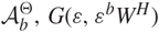 $ ({\varepsilon ^b}(\rho B + \overline \rho {B^ \bot }),{Y^\varepsilon }) = ({\varepsilon ^b}(\rho B + \overline \rho {B^ \bot }),G(\varepsilon ,{\varepsilon ^b}{W^H})(t)) $. Moreover, using
 ${\cal A}_b^\Theta ,G(\varepsilon ,{\varepsilon ^b}{W^H})$ is exponentially equivalent to
 $\overline G ({\varepsilon ^b}{W^H})$, with
 $\overline G (\varphi )(t){\kern 1pt} : = {\kern 1pt} \xi \int_0^t {e^{\beta (t - u)}}{\kern 1pt} d{\varphi _u}$. The contraction principle thus yields
 $ ({\varepsilon ^b}(\rho B + \overline \rho {B^ \bot }),{Y^\varepsilon }) \sim LDP({\varepsilon ^{2b}},{I_4}) $, with
 ${I_4}{\kern 1pt} :{\kern 1pt} (\varphi ,\psi ) \mapsto \inf \{ {I_3}(\varphi ,v)\;|\;\psi \in {\cal C}{\kern 1pt} :{\kern 1pt} \psi = \overline G (v)\} $.
Under 𝒜 ′, the extended contraction principle [Reference Mayer-Wolf, Nualart and PéRez-Abreu40, Proposition 2.3] yields that  $ ({\varepsilon ^b}(\rho B{\kern 1pt} + {\kern 1pt} \overline \rho ){B^ \bot },\widetilde\sigma ({Y^\varepsilon })) \sim LDP({\varepsilon ^{2b}},{I_5}) $ with
 ${I_5}(\varphi ,\psi ){\kern 1pt} : = {\kern 1pt} \inf \{ {I_4}(\varphi ,v)\;|\;\psi = \widetilde\sigma (v)\} = \inf \{ {I_3}(\varphi ,v){\kern 1pt} |\psi = \widetilde\sigma (\overline G (v))\} $. Finally, setting
 $b \ge {1 \over 2}$, the sequence of semi-martingales (εbW) is uniformly exponentially tight (UET) in the sense of [Reference Garcia28, Definition 1.1], and the sequence
 $(\widetilde\sigma ({Y^\varepsilon }))$ is continuous from the right with no left limits (càdlàg; Assumption 𝒜), and adapted to the filtration ℱ. Denoting by X ⋅ Y := ∫X dY the stochastic integral with respect to a semi-martingale, Theorem 1.2 in [Reference Garcia28] yields a large deviations principle on 𝒞(𝒯, ℝ3) for
 $({\varepsilon ^b}(\rho {B_s}{\kern 1pt} + {\kern 1pt} \overline \rho B_s^ \bot ),\widetilde\sigma ({Y^\varepsilon }),{\varepsilon ^b}\int_0^ \cdot \widetilde\sigma (Y_s^\varepsilon )(\rho d{B_s} + \overline \rho dB_s^ \bot ))$, with speed ε 2b and good rate function I 6 defined as I 6(ϕ) := I 5(φ, ψ) if ϕ = φ ⋅ ψ and ψ ∈ BV (the space of functions of finite variation), and infinity otherwise. Since, for t ∈ 𝒯 *,
 $$\tilde X_t^\varepsilon = - {1 \over 2}\int_0^t \widetilde\sigma {(Y_s^\varepsilon )^2}{\kern 1pt} ds + \int_0^t {\varepsilon ^b}\widetilde\sigma (Y_s^\varepsilon ){\kern 1pt} d{W_s}{\kern 1pt} = :{\kern 1pt} I(\widetilde\sigma ({Y^\varepsilon }),\widetilde\sigma ({Y^\varepsilon }) \cdot {\varepsilon ^b}(\rho {B_s} + \overline \rho B_s^ \bot ))(\varepsilon ,t),$$
the contraction principle then yields  ${\tilde X^\varepsilon } \sim LDP({\varepsilon ^{2b}},\widetilde\Lambda )$ with
 $$\widetilde\Lambda (\phi ){\kern 1pt} : = {\kern 1pt} \inf \{ {I_6}(\chi )\;|\;\phi = I(\varphi ,\varphi \cdot \psi ),\chi = (\varphi ,\psi ),\psi \in BV\} .$$
It remains to prove that Xε and  ${\tilde X^\varepsilon }$ are exponentially equivalent. Indeed, for t ∈ 𝒯 *,
 $$\matrix{
{\parallel {X^\varepsilon } - {{\tilde X}^\varepsilon }{\parallel _\infty }} & \le & {{1 \over 2}\parallel \int_0^ \cdot |{\varepsilon ^{2b}}{\sigma ^2}({{Y_s^\varepsilon } \over {{\varepsilon ^b}}}) - \widetilde\sigma (Y_s^\varepsilon )|ds{\parallel _\infty }} \cr
{} & {} & {\quad + {\varepsilon ^b}\parallel \int_0^ \cdot |{\varepsilon ^b}\sigma ({{Y_s^\varepsilon } \over {{\varepsilon ^b}}}) - \widetilde\sigma (Y_s^\varepsilon )|d(\rho {B_s} + \overline \rho B_s^ \bot ){\parallel _\infty }.} \cr
} $$
Using the linear growth assumption as well as Assumption 𝒜, we have, for s ∈ [0, t],
 $$\matrix{
{|{\varepsilon ^{2b}}{\sigma ^2}({{Y_s^\varepsilon } \over {{\varepsilon ^b}}}) - \widetilde\sigma (Y_s^\varepsilon )|} \hfill & \le \hfill & {2{C^2}\{ {\varepsilon ^{2b}}[1 + |{{Y_s^\varepsilon } \over {{\varepsilon ^b}}}{|^2}] + 1 + |Y_s^\varepsilon {|^2}\} } \hfill \cr
{} \hfill & \le \hfill & {2{C^2}[1 + {\varepsilon ^{2b}} + 2|Y_s^\varepsilon {|^2}],} \hfill \cr
} $$
and hence
 $$\matrix{
{\parallel \int_0^ \cdot |{\varepsilon ^{2b}}{\sigma ^2}({{Y_s^\varepsilon } \over {{\varepsilon ^b}}}) - \widetilde\sigma (Y_s^\varepsilon )|ds{\parallel _\infty }} \hfill & \le \hfill & {\parallel \int_0^ \cdot 2{C^2}(1 + {\varepsilon ^{2b}} + 2|Y_s^\varepsilon {|^2})ds{\parallel _\infty }} \hfill \cr
{} \hfill & \le \hfill & {2{C^2}(1 + {\varepsilon ^{2b}}) + 4{C^2}\parallel \int_0^ \cdot |Y_s^\varepsilon {|^2}{\kern 1pt} ds{\parallel _\infty }.} \hfill \cr
} $$
Since  $Y_s^\varepsilon = {\varepsilon ^b}{e^{\beta s}}\Theta + {\varepsilon ^b}{\lambda \over \beta }({e^{\beta s}} - 1) + {\varepsilon ^b}\xi [W_s^H + \beta \int_0^s W_u^H{e^{ - \beta u}}{\kern 1pt} du]$, we obtain, for s ∈ 𝒯,
 $|Y_s^\varepsilon | \le {\varepsilon ^b}{e^{\beta s}}|\Theta | + {\varepsilon ^b}{\lambda \over \beta }({e^{\beta s}} - 1) + \xi {\varepsilon ^b}|W_s^H|,$, because β < 0, and
 $$|Y_s^\varepsilon {|^2} \le 2({\varepsilon ^{2b}}{e^{2\beta s}}{\Theta ^2} + 2{\varepsilon ^{2b}}{({\lambda \over \beta })^2}({e^{2\beta s}} + 1) + {\xi ^2}{\varepsilon ^{2b}}|W_s^H{|^2}),$$
so that
 $$\int_0^t |Y_s^\varepsilon {|^2}{\kern 1pt} ds \le 2({\varepsilon ^{2b}}t{\Theta ^2} + {\varepsilon ^{2b}}{({\lambda \over \beta })^2}(2t - {1 \over \beta }) + {\xi ^2}{\varepsilon ^{2b}}\int_0^t |W_s^H{|^2}{\kern 1pt} ds).$$
Introduce
 $${\cal J}{\kern 1pt} : = {\kern 1pt} 2{C^2}\parallel \int_0^ \cdot |Y_s^\varepsilon {|^2}{\kern 1pt} ds{\parallel _\infty }\quad \quad {\rm{and}}\quad \quad \Xi _s^\varepsilon {\kern 1pt} : = {\kern 1pt} {\varepsilon ^b}\sigma ({{Y_s^\varepsilon } \over {{\varepsilon ^b}}}) - \widetilde\sigma (Y_s^\varepsilon ).$$
For any δ, a 0 > 0, we can then write
 $$\matrix{
{P[\parallel {X^\varepsilon } - {{\tilde X}^\varepsilon }{\parallel _\infty } > \delta ]} \hfill & { \le P[{\cal J} + {\varepsilon ^b}\parallel \int_0^ \cdot \Xi _s^\varepsilon d(\rho {B_s} + \overline \rho B_s^ \bot ){\parallel _\infty } > {\delta _\varepsilon }]} \hfill \cr
{} \hfill & { \le P[{\cal J} + {\varepsilon ^b}\parallel \int_0^ \cdot \Xi _s^\varepsilon d(\rho {B_s} + \overline \rho B_s^ \bot ){\parallel _\infty } > {\delta _\varepsilon }|{\cal J} \lt {a_0}](1 - )} \hfill \cr
{} \hfill & { + P[{\cal J} + {\varepsilon ^b}\parallel \int_0^ \cdot \Xi _s^\varepsilon d(\rho {B_s} + \overline \rho B_s^ \bot ){\parallel _\infty } > {\delta _\varepsilon }|{\cal J} \ge {a_0}]} \hfill \cr
{} \hfill & { \le P[\parallel \int_0^ \cdot \Xi _s^\varepsilon d(\rho {B_s} + \overline \rho B_s^ \bot ){\parallel _\infty } > {{{\delta _\varepsilon } - {a_0}} \over {{\varepsilon ^b}}}|{\cal J} \lt {a_0}] + ,} \hfill \cr
} $$
with 𝔓 := P(𝒥 ≥ a 0), δε := δ − C 2(1 + ε 2b). Let  ${{\cal J}_t}{\kern 1pt} : = {\kern 1pt} \int_0^t |W_s^H{|^2}{\kern 1pt} ds$. By (A.3), we have
 $$\matrix{
{P({\cal J} > \bar \delta )} \hfill & { \le P(|{\varepsilon ^{2b}}{\Theta ^2} + {\varepsilon ^{2b}}{{({\lambda \over \beta })}^2}(2 - {1 \over \beta }) + {\xi ^2}{\varepsilon ^{2b}}{{\cal J}_1}| > {{\bar \delta } \over 2})} \hfill \cr
{} \hfill & { \le P({\varepsilon ^{2b}}{\Theta ^2} + {\varepsilon ^{2b}}{{({\lambda \over \beta })}^2}|2 - {1 \over \beta }| + {\xi ^2}{\varepsilon ^{2b}}{{\cal J}_1} > {{\bar \delta } \over 2}|{\xi ^2}{\varepsilon ^{2b}}{{\cal J}_1} \lt a)} \hfill \cr
{} \hfill & {\quad \times P({\xi ^2}{\varepsilon ^{2b}}{{\cal J}_1} \lt a)} \hfill \cr
{} \hfill & {\quad + P({\varepsilon ^{2b}}{\Theta ^2} + {\varepsilon ^{2b}}{{({\lambda \over \beta })}^2}|2 - {1 \over \beta }| + {\xi ^2}{\varepsilon ^{2b}}{{\cal J}_1} > {{\bar \delta } \over 2}|{\xi ^2}{\varepsilon ^{2b}}{{\cal J}_1} \ge a)} \hfill \cr
{} \hfill & {\quad \quad \times P({\xi ^2}{\varepsilon ^{2b}}{{\cal J}_1} \ge a)} \hfill \cr
{} \hfill & { \le P({\Theta ^2} > {1 \over {{\varepsilon ^{2b}}}}({{\bar \delta } \over 2} - {\varepsilon ^{2b}}{{({\lambda \over \beta })}^2}|2 - {1 \over \beta }| - a)|{\xi ^2}{\varepsilon ^{2b}}{{\cal J}_1} \lt a)} \hfill \cr
{} \hfill & {\quad + P({\xi ^2}{\varepsilon ^{2b}}{{\cal J}_1} \ge a)} \hfill \cr
{} \hfill & { \le P(|\Theta | > {1 \over {{\varepsilon ^b}}}\sqrt {({{\bar \delta } \over 2} - {\varepsilon ^{2b}}{{({\lambda \over \beta })}^2}|2 - {1 \over \beta }| - a)} |{\xi ^2}{\varepsilon ^{2b}}{{\cal J}_1} \lt a)} \hfill \cr
{} \hfill & {\quad + P({\xi ^2}{\varepsilon ^{2b}}{{\cal J}_1} \ge a),} \hfill \cr
} $$
for any  $\bar \delta > 0$ and a > 0. One can then use Markov’s inequality:
 $$P({\xi ^2}{\varepsilon ^{2b}}{{\cal J}_1} \ge a) \le {{E[{\xi ^2}{\varepsilon ^{2b}}{{\cal J}_1}]} \over a} = {{{\xi ^2}{\varepsilon ^{2b}}} \over a}E(\int_0^1 |W_s^H{|^2}{\kern 1pt} ds).$$
Since 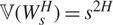 ${\mathbb {V}}(W_{s}^{H}) = {s^{2H}}$, one obtains
 $P({\xi ^2}{\varepsilon ^{2b}}{{\cal J}_1} \ge a) \le {{{\xi ^2}{\varepsilon ^{2b}}} \over a}{1 \over {2H + 1}}.$. Hence there exist η ∈ [0, 1) and
 $\bar \varepsilon > 0$ such that for all
 $\varepsilon \le \bar \varepsilon $, P(ξ 2ε 2b 𝒥 1 < a) ≥ 1 − η. Assumption
 ${\cal A}_b^\Theta $ then implies that there exist M,
 $\tilde \varepsilon > 0$ such that
 $$P(|\Theta | > {1 \over {{\varepsilon ^b}}}\sqrt {({{\bar \delta } \over 2} - {\varepsilon ^{2b}}{{({\lambda \over \beta })}^2}|2 - {1 \over \beta }| - a)} ) \le \exp ( - {M \over {{\varepsilon ^{2b}}}}),\quad \quad {\rm{forall}}\varepsilon \le \tilde \varepsilon .$$
Thus, for all  $\varepsilon \le \min \{ \tilde \varepsilon ,\bar \varepsilon \} $, Bayes’ Theorem yields
 $$\matrix{
{P(|\Theta | > {1 \over {{\varepsilon ^b}}}\sqrt {({{\bar \delta } \over 2} - {\varepsilon ^{2b}}{{({\lambda \over \beta })}^2}|2 - {1 \over \beta }| - a)} |{\xi ^2}{\varepsilon ^{2b}}{{\cal J}_1} \lt a)} \cr
{ \le {{P(|\Theta | > {1 \over {{\varepsilon ^b}}}\sqrt {({{\bar \delta } \over 2} - {\varepsilon ^{2b}}{{({\lambda \over \beta })}^2}|2 - {1 \over \beta }| - a)} )} \over {P({\xi ^2}{\varepsilon ^{2b}}{{\cal J}_1} \lt a)}} \le {{\exp ( - {M \over {{\varepsilon ^{2b}}}})} \over {1 - \eta }}.} \cr
} $$
Finally, for all  $\varepsilon \le \min \{ \tilde \varepsilon ,\bar \varepsilon \} $,
 $$\matrix{
{P({\cal J} > \bar \delta )} \hfill & \le \hfill & {P(|\Theta | > {1 \over {{\varepsilon ^b}}}\sqrt {({{\bar \delta } \over 2} - {\varepsilon ^{2b}}{{({\lambda \over \beta })}^2}|2 - {1 \over \beta }| - a)} |{\xi ^2}{\varepsilon ^{2b}}{{\cal J}_1} \lt a)} \hfill \cr
{} \hfill & {} \hfill & {\quad + P({\xi ^2}{\varepsilon ^{2b}}{{\cal J}_1} \ge a)} \hfill \cr
{} \hfill & \le \hfill & {{{{e^{ - M/{\varepsilon ^{2b}}}}} \over {1 - \eta }} + {{{\xi ^2}{\varepsilon ^{2b}}} \over a}{1 \over {2{H_ + }}},} \hfill \cr
} $$
so that for all  $\varepsilon \le \min \{ \tilde \varepsilon ,\bar \varepsilon \} $,
 $P({\cal J} \ge {a_0}) \le {{{e^{ - M/{\varepsilon ^{2b}}}}} \over {1 - \eta }} + {{{\xi ^2}{\varepsilon ^{2b}}} \over a}{1 \over {2{H_ + }}}$. Hence, there exist
 $\mathord{\buildrel{\lower3pt\hbox{$\scriptscriptstyle\smile$}}\over \eta } \in [0,1)$,
 $$\mathord{\buildrel{\lower3pt\hbox{$\scriptscriptstyle\smile$}}\over
\varepsilon } \lt \tilde \varepsilon \wedge \bar \varepsilon $$ such that
 $$P({\cal J} \lt {a_0}) \ge 1 - \mathord{\buildrel{\lower3pt\hbox{$\scriptscriptstyle\smile$}}\over
\eta } $$ for all
 $$\varepsilon \le \mathord{\buildrel{\lower3pt\hbox{$\scriptscriptstyle\smile$}}\over
\varepsilon } $$. By the uniform convergence assumed in 𝒜, for all y ∈ ℝ there exist N, ε 0 > 0 such that
 $|{\varepsilon ^b}\sigma ({{Y_s^\varepsilon } \over {{\varepsilon ^b}}}) - \widetilde\sigma (Y_s^\varepsilon )| \le N$ for all ε < ε 0. The Borell–TIS inequality [Reference Peithmann47, Proposition A.1] then yields
 $$\matrix{
{P(\parallel \int_0^ \cdot ({\varepsilon ^b}\sigma ({{Y_s^\varepsilon } \over {{\varepsilon ^b}}}) - \widetilde\sigma (Y_s^\varepsilon ))d(\rho {B_s} + \overline \rho B_s^ \bot ){\parallel _\infty } > {1 \over {{\varepsilon ^b}}}(\delta - {C^2}(1 + {\varepsilon ^{2b}}) - {a_0}))} \hfill \cr
{ \le 2\exp \{ - {{{{(\delta - {C^2}(1 + {\varepsilon ^{2b}}) - {a_0})}^2}} \over {2{N^2}{\varepsilon ^{2b}}}}\} .} \hfill \cr
} $$
Thus, for all  $$\varepsilon \le \min \{ \mathord{\buildrel{\lower3pt\hbox{$\scriptscriptstyle\smile$}}\over
\varepsilon } ,{\varepsilon _0}\} $$, Bayes’ Theorem yields
 $$\matrix{
{} \hfill & {P(\parallel \int_0^ \cdot \Xi _s^\varepsilon d(\rho {B_s} + \overline \rho B_s^ \bot ){\parallel _\infty } > {{\delta - {C^2}(1 + {\varepsilon ^{2b}}) - {a_0}} \over {{\varepsilon ^b}}}|{\cal J} \lt {a_0})} \hfill \cr
{} \hfill & { \le {{P(\parallel \int_0^ \cdot \Xi _s^\varepsilon d(\rho {B_s} + \overline \rho B_s^ \bot ){\parallel _\infty } > {{\delta - {C^2}(1 + {\varepsilon ^{2b}}) - {a_0}} \over {{\varepsilon ^b}}})} \over {P({\cal J} \lt {a_0})}}} \hfill \cr
{} \hfill & { \le {2 \over {1 - \mathord{\buildrel{\lower3pt\hbox{$\scriptscriptstyle\smile$}}\over
\eta } }}\exp \{ - {{{{(\delta - {C^2}(1 + {\varepsilon ^{2b}}) - {a_0})}^2}} \over {2{N^2}{\varepsilon ^{2b}}}}\} .} \hfill \cr
} $$
Finally, for all  $$\varepsilon \le \min \{ \mathord{\buildrel{\lower3pt\hbox{$\scriptscriptstyle\smile$}}\over
\varepsilon } ,{\varepsilon _0}\} $$,
 $$P(\parallel {X^\varepsilon } - {\tilde X^\varepsilon }{\parallel _\infty } > \delta ) \le {{2\exp \{ - {{{{(\delta - {C^2}(1 + {\varepsilon ^{2b}}) - {a_0})}^2}} \over {2{N^2}{\varepsilon ^{2b}}}}\} } \over {1 - \mathord{\buildrel{\lower3pt\hbox{$\scriptscriptstyle\smile$}}\over
\eta } }} + {{{e^{ - M/{\varepsilon ^{2b}}}}} \over {1 - \eta }} + {{{\xi ^2}{\varepsilon ^{2b}}} \over {2a{H_ + }}},$$
so that Xε and  ${\tilde X^\varepsilon }$ are exponentially equivalent and
 ${X^\varepsilon } \sim LDP({\varepsilon ^{2b}},\widetilde\Lambda )$.
Remark A.1. For computational purposes, such infinite-dimensional optimisation problems are discretised over a set of basis functions, such as orthonormal polynomials. If we then consider φ continuously differentiable and I 1 finite, we can simplify  ${I_1}(\varphi ) = {I_1}(\varphi ,\psi ) = {1 \over {2{\rho ^2}}}\int_{\cal T} {[\dot \varphi (t)]^2}{\kern 1pt} dt$. Further, if u ∈ 𝒞 1, then I 4(φ) = I 3(φ) and
 $${I_3}(\varphi ) \simeq {1 \over 2}\mathop {\inf }\limits_{u \in {\cal H} \cap {{\cal C}^1}} \{ \int_0^t {({{{{\dot u}_s}} \over \rho })^2}ds + {1 \over {\overline \rho }}\int_0^t {({\dot \varphi _s} - {\dot u_s})^2}{\kern 1pt} ds\} .$$
A.2. Proof of Theorem 3.4
A.2.1. Proof of Theorem 3.4(i)
Let us introduce the process  ${\overline Y ^\varepsilon }$ defined, for t ∈ 𝒯 *, as the unique solution of
 $d\overline Y _t^\varepsilon = ({\varepsilon ^{b + 2}}\lambda + \beta {\varepsilon ^2}\overline Y _t^\varepsilon )d\tau + {\varepsilon ^{2H + b}}\xi dW_t^H$, with
 $\overline Y _0^\varepsilon = 0$, i.e.
 $$\overline Y _t^\varepsilon = - {{\lambda {\varepsilon ^b}} \over \beta }(1 - {e^{\beta {\varepsilon ^2}t}}) + \xi {\varepsilon ^{2H + b}}\int_0^t {e^{\beta {\varepsilon ^2}(t - u)}}{\kern 1pt} dW_u^H.$$
By Lemma 3.1, Proposition 3.2, and [Reference Deuschel and Stroock19, Theorem 3.4.5], the sequence
 $${({\varepsilon ^{2H + b}}\int_0^ \cdot G_0^H( \cdot ,s){\kern 1pt} d{Z_s})_{\varepsilon > 0}}$$
satisfies an LDP on 𝒞, with speed ε 4H+2b and good rate function  ${\Lambda _{G_0^H}}$ as in (2.4). Also:
(1) When
$H \ne {1 \over 2}$, ${({\varepsilon ^{2H + b}}\int_0^t G_\varepsilon ^H(t,s){\kern 1pt} d{Z_s})_{\varepsilon > 0}}$ and ${({\varepsilon ^{2H + b}}\int_0^t G_0^H(t,s){\kern 1pt} d{Z_s})_{\varepsilon > 0}}$ are exponentially equivalent: indeed, the asymptotic expansion of the Gaussian density [Reference Abramowitz and Stegun1, Formula (26.2.12)] yields, for any δ > 0,$$\matrix{
{P[\parallel {\varepsilon ^{2H + b}}\int_0^ \cdot G_\varepsilon ^H( \cdot ,s){\kern 1pt} d{Z_s} - {\varepsilon ^{2H + b}}\int_0^ \cdot G_0^H( \cdot ,s){\kern 1pt} d{Z_s}{\parallel _\infty } > \delta ]} \hfill \cr
{ = P[\parallel \int_0^ \cdot (G_\varepsilon ^H( \cdot ,s) - G_0^H( \cdot ,s))d{Z_s}{\parallel _\infty } > {\delta \over {{\varepsilon ^{2H + b}}}}] = P[|{\cal N}(0,1)| > {{\delta {\varepsilon ^{ - 2H - b}}} \over {\parallel {V_\varepsilon }{\parallel _\infty }}}]} \hfill \cr
{ = \sqrt {{2 \over \pi }} {{\parallel {V_\varepsilon }{\parallel _\infty }{\varepsilon ^{2H + b}}} \over \delta }\exp ( - {{{\delta ^2}} \over {2{\varepsilon ^{4H + 2b}}\parallel {V_\varepsilon }\parallel _\infty ^2}})(1 + {\cal O}({\varepsilon ^{4H + 2b}})),} \hfill \cr
} $$
with
$V_\varepsilon ^2{\kern 1pt} : = {\kern 1pt} \int_0^t {(G_\varepsilon ^H(t,s) - G_0^H(t,s))^2}ds$; note that $\mathop {\lim }\nolimits_{\varepsilon \downarrow 0} V_\varepsilon ^2 = 0$. Now, for ε > 0 and 0 < s < t,(i) if
$H \lt {1 \over 2}$$$\matrix{
{{{[G_\varepsilon ^H(t,s) - G_0^H(t,s)]}^2}} \hfill & \le \hfill & {{{2\kappa _H^2{\xi ^2}} \over {{s^{2{H_ - }}}}}\{ {H_ - }^2{{(\int_s^t {{{{(u - s)}^{{H_ - }}}} \over {{u^{1 - {H_ - }}}}}({e^{\beta {\varepsilon ^2}(t - u)}} - 1)du)}^2}.} \hfill \cr
{} \hfill & {} \hfill & {\quad . + {\beta ^2}{\varepsilon ^4}{{(\int_s^t {{(u - s)}^{{H_ - }}}{u^{{H_ - }}}{e^{\beta {\varepsilon ^2}(t - u)}}{\kern 1pt} du)}^2}\} } \hfill \cr
{} \hfill & \le \hfill & {2\kappa _H^2{\xi ^2}[{{{H_ - }^2} \over {{s^{2{H_ - }}}}}{{(\int_s^t {{{{(u - s)}^{{H_ - }}}} \over {{u^{1 - {H_ - }}}}}{\kern 1pt} du)}^2}} \hfill \cr
{} \hfill & {} \hfill & {\quad \quad \quad \quad \quad + {{{\beta ^2}{\varepsilon ^4}} \over {{s^{2{H_ - }}}}}{{(\int_s^t {{(u(u - s))}^{{H_ - }}}{\kern 1pt} du)}^2}]} \hfill \cr
} $$
Using [Reference Yan, Lu and Xu53, Lemma A.3], we further obtain, for ε > 0 and 0 < s < t,
$V_\varepsilon ^2 \le 2\kappa _H^2{\xi ^2}[{C_H}{t^{2H}} + {\beta ^2}{\varepsilon ^4}{\tilde C_H}{t^{2H + 2}}]$, with CH, ${\tilde C_H} > 0$. Hence,$$0 \lt {\varepsilon ^{4H + 2b}}V_\varepsilon ^2 \le 2\kappa _H^2{\xi ^2}({C_H}{\varepsilon ^{4H + 2b}}{t^{2H}} + {\beta ^2}{\varepsilon ^{4H + 2b + 4}}{\tilde C_H}{t^{2H + 2}});$$
(ii) if
$H > {1 \over 2}$$$\matrix{
{{{[G_\varepsilon ^H(t,s) - G_0^H(t,s)]}^2}} \hfill & = \hfill & {{{\kappa _H^2{\xi ^2}} \over {{s^{2{H_ - }}}}}{H_ - }^2{{(\int_s^t {{{u^{{H_ - }}}} \over {{{(u - s)}^{1 - {H_ - }}}}}({e^{\beta {\varepsilon ^2}(t - u)}} - 1){\kern 1pt} du)}^2}} \hfill \cr
{} \hfill & \le \hfill & {{{\kappa _H^2{\xi ^2}} \over {{s^{2{H_ - }}}}}{H_ - }^2{{(\int_s^t {{{u^{{H_ - }}}{\kern 1pt} du} \over {{{(u - s)}^{1 - {H_ - }}}}})}^2}} \hfill \cr
{} \hfill & \le \hfill & {{{\kappa _H^2{\xi ^2}} \over {{s^{2{H_ - }}}}}{H_ - }^2{t^{2{H_ - }}}{{(\int_s^t {{(u - s)}^{{H_ - } - 1}}{\kern 1pt} du)}^2}} \hfill \cr
{} \hfill & = \hfill & {{{\kappa _H^2{\xi ^2}} \over {{s^{2{H_ - }}}}}{{[t(t - s)]}^{2{H_ - }}}.} \hfill \cr
} $$
Hence, for
$H \ne {1 \over 2}$, as b > 0,$$\mathop {\lim }\limits_{\varepsilon \downarrow 0} {\varepsilon ^{4H + 2b}}\parallel {V_\varepsilon }\parallel _\infty ^2 = 0{\rm{and}}\mathop {\lim }\limits_{\varepsilon \downarrow 0} {\varepsilon ^{2H + b}}\parallel {V_\varepsilon }{\parallel _\infty } = 0.$$
(2) When
$H = {1 \over 2}$, ${(\xi {\varepsilon ^{1 + b}}\int_0^t {e^{\beta {\varepsilon ^2}(t - s)}}{\kern 1pt} d{B_s})_{\varepsilon > 0}}$ and (ξε 1+bBt)ε>0 are exponentially equivalent: the asymptotic expansion of the Gaussian density near infinity [Reference Abramowitz and Stegun1, Formula (26.2.12)] yields, for any δ > 0,$$\matrix{
{P(\parallel \xi \int_0^ \cdot {e^{\beta {\varepsilon ^2}( \cdot - s)}}{\kern 1pt} d{B_s} - \xi \int_0^ \cdot d{B_s}{\parallel _\infty } > {\delta \over {{\varepsilon ^{1 + b}}}})} \hfill \cr
{ = P(\parallel \int_0^ \cdot \xi ({e^{\beta {\varepsilon ^2}( \cdot - s)}} - 1)d{B_s}{\parallel _\infty } > {\delta \over {{\varepsilon ^{1 + b}}}})} \hfill \cr
{ = P(|{\cal N}(0,1)| > {\delta \over {\parallel {V_\varepsilon }{\parallel _\infty }{\varepsilon ^{1 + b}}\xi }})} \hfill \cr
{ = \sqrt {{2 \over \pi }} {{\parallel {V_\varepsilon }{\parallel _\infty }{\varepsilon ^{1 + b}}\xi } \over \delta }\exp ( - {{{\delta ^2}} \over {2{\varepsilon ^{2 + 2b}}\parallel {V_\varepsilon }\parallel _\infty ^2{\xi ^2}}})(1 + {\cal O}({\varepsilon ^{2 + 2b}})),} \hfill \cr
} $$
with
$$V_\varepsilon ^2{\kern 1pt} : = {\kern 1pt} \int_0^t {[({e^{\beta {\varepsilon ^2}(t - s)}} - 1)]^2}ds = t + {{{e^{2\beta {\varepsilon ^2}t}} - 1} \over {2\beta {\varepsilon ^2}}} + {{2(1 - {e^{\beta {\varepsilon ^2}t}})} \over {\beta {\varepsilon ^2}}}.$$
Hence
$0 \lt {\varepsilon ^{2 + 2b}}V_\varepsilon ^2 \le {\varepsilon ^{2 + 2b}}t + {\varepsilon ^{2b}}{{{e^{\beta {\varepsilon ^2}t}} - 1} \over {2\beta }},$, and, as b > 0, $\mathop {\lim }\nolimits_{\varepsilon \downarrow 0} {\varepsilon ^{2 + 2b}}\parallel {V_\varepsilon }\parallel _\infty ^2 = 0$. Also, note that $\mathop {\lim }\nolimits_{\varepsilon \downarrow 0} V_\varepsilon ^2 = 0$. The required exponential equivalence then follows, and hence for all ${({\varepsilon ^{2H + b}}\int_0^ \cdot G_\varepsilon ^H( \cdot ,s){\kern 1pt} d{Z_s})_{\varepsilon > 0}} \sim LDP({\varepsilon ^{4H + 2b}},{\Lambda _{G_0^H}})$.The final step is exponential equivalence between
${({\varepsilon ^{2H + b}}\int_0^ \cdot G_\varepsilon ^H( \cdot ,s){\kern 1pt} d{Z_s})_{\varepsilon > 0}}$ and ${\overline Y ^\varepsilon }$. For any δ, t > 0,$$\matrix{
{P(\parallel {{\overline Y }^\varepsilon } - {\varepsilon ^{2H + b}}\int_0^ \cdot G_\varepsilon ^H( \cdot ,s){\kern 1pt} d{Z_s}{\parallel _\infty } > \delta )} \hfill \cr
{ = P(\parallel {{\overline Y }^\varepsilon } - {\varepsilon ^{2H + b}}\int_0^ \cdot {e^{\beta {\varepsilon ^2}( \cdot - s)}}{\kern 1pt} dW_s^H{\parallel _\infty } > \delta )} \hfill \cr
{ = P(\parallel - {{\lambda {\varepsilon ^b}} \over \beta }(1 - {e^{\beta {\varepsilon ^2} \cdot }}){\parallel _\infty } > \delta ).} \hfill \cr
} $$
Hence,
$$\mathop {\limsup }\limits_{\varepsilon \downarrow 0} {\varepsilon ^{4H + 2b}}\log P(\parallel {\overline Y ^\varepsilon } - {\varepsilon ^{2H + b}}\int_0^ \cdot {G_\varepsilon }( \cdot ,s){\kern 1pt} d{Z_s}{\parallel _\infty } > \delta ) = - \infty ,$$
yielding exponential equivalence and
${\overline Y ^\varepsilon } \sim LDP({\varepsilon ^{4H + 2b}},{\Lambda _{G_0^H}})$. Finally, since$$P(\parallel {Y^\varepsilon } - {\overline Y ^\varepsilon }{\parallel _\infty } > \delta ) \le P({\varepsilon ^b}|\Theta | > \delta ),$$
for any δ > 0 as β < 0, and
${\overline Y ^\varepsilon }$ and Yε are exponentially equivalent, and ${Y^\varepsilon } \sim LDP({\varepsilon ^{4H + 2b}},{\Lambda _{G_0^H}})$ by Assumption ${\cal A}_b^\Theta $.





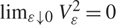










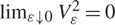









A.2.2. Proof of Theorem 3.4(ii)
The proof is similar to that of Theorem 3.1(ii).
(1)
$H \ne {1 \over 2}$ : we have already established that ${\varepsilon ^{2H + b}}(\overline \rho {B^ \bot } + \rho B,{W^H})$ satisfies a large deviations principle on 𝒞(𝒯, ℝ2), with speed ε 4H+2b and good rate function I 3 defined earlier.(2)
$H = {1 \over 2}$ : using the proof of Theorem 3.3, ${\varepsilon ^{b + 1}}(\overline \rho {B^ \bot } + \rho B,B)'$ satisfies a large deviations principle on 𝒞(𝒯, ℝ2), with speed ε 2+2b and good rate function Λρ defined in (3.5).




Similar to above, we only prove the case  $H \ne {1 \over 2}$, the other one being analogous. We introduce the process
 ${\tilde X^\varepsilon }$ satisfying the SDE
 $d\tilde X_t^\varepsilon = - {{{\varepsilon ^{2H + 1}}} \over 2}{\widetilde\sigma ^2}(Y_t^\varepsilon )dt + {\varepsilon ^{2H + b}}\widetilde\sigma (Y_t^\varepsilon )(\rho d{B_t} + \overline \rho dB_t^ \bot )$, and translate this large deviations case into one for the sequence
 ${\tilde X^\varepsilon }$. Using that for ε > 0 and t ∈ 𝒯 *,
 $Y_t^\varepsilon = {\varepsilon ^b}{e^{\beta {\varepsilon ^2}t}}\Theta - {{\lambda {\varepsilon ^b}} \over \beta }(1 - {e^{\beta {\varepsilon ^2}t}}) + {\varepsilon ^{2H + b}}\xi \int_0^t {e^{\beta {\varepsilon ^2}(t - u)}}{\kern 1pt} dW_u^H$, one can define a continuous map
 $\tilde G((0,1) \times {\cal C} \to {\cal C})$ such that
 $({\varepsilon ^{2H + b}}(\rho B + \overline \rho {B^ \bot }),{Y^\varepsilon }) = ({\varepsilon ^{2H + b}}(\rho B{\kern 1pt} + {\kern 1pt} \overline \rho {B^ \bot }),\tilde G(\varepsilon ,{\varepsilon ^{2H + b}}{W^H})(t))$. Using
 ${\cal A}_b^\Theta $ and the asymptotic expansion of the Gaussian density near infinity [Reference Abramowitz and Stegun1, Formula (26.2.12)],
 $\tilde G(\varepsilon ,{\varepsilon ^{2H + b}}{W^H})$ is exponentially equivalent to
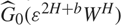 ${\hat G_0}({\varepsilon ^{2H + b}}{W^H})$, defined by
 ${\hat G_0}(\varphi )(t){\kern 1pt} : = {\kern 1pt} \xi \int_0^t d{\varphi _u}$.
Hence, the contraction principle yields an LDP on 𝒞(𝒯, ℝ2) for  $({\varepsilon ^{2H + b}}(\rho B + \overline \rho {B^ \bot }),{Y^\varepsilon })$, with speed ε 4H+2b and good rate function
 ${\tilde I_4}{\kern 1pt} :{\kern 1pt} (\varphi ,\psi ) \mapsto \inf \{ {I_3}(\varphi ,v)\;|\;\psi \in {\cal C}{\kern 1pt} :{\kern 1pt} \psi = {\hat G_0}(v)\} $. Under 𝒜 ′, the extended contraction principle [Reference Mayer-Wolf, Nualart and PéRez-Abreu40, Proposition 2.3] yields an LDP on 𝒞(𝒯, ℝ2) for
 $({\varepsilon ^{2H + b}}(\rho B + \overline \rho {B^ \bot }),\widetilde\sigma ({Y^\varepsilon }))$, with speed ε 4H+2b and good rate function
 ${\tilde I_5}{\kern 1pt} :{\kern 1pt} (\varphi ,\psi ) \mapsto \inf \{ {\tilde I_4}(\varphi ,v)\;|\;\psi = \widetilde\sigma (v)\} = \inf \{ {I_3}(\varphi ,v)\;|\;\psi = \widetilde\sigma ({\hat G_0}(v))\} $. Finally, setting
 $b \ge {1 \over 2} - 2H$, the sequence of semi-martingales (ε 2H+bW) is UET and the sequence
 $(\widetilde\sigma ({Y^\varepsilon }))$ is càdlàg (Assumption 𝒜), and adapted to the filtration ℱ. Theorem 1.2 in [Reference Garcia28] thus gives an LDP on 𝒞 for the sequence of stochastic integrals
 ${\varepsilon ^{2H + b}}\int_0^ \cdot \widetilde\sigma (Y_s^\varepsilon )(\rho d{B_s} + \overline \rho dB_s^ \bot )$, with speed ε 4H+2b and good rate function
 $$I(\chi ){\kern 1pt} : = {\kern 1pt} \inf \{ {\tilde I_5}(\varphi ,\psi ){\kern 1pt} :{\kern 1pt} \varphi \cdot \psi = \chi ,\;\psi \in BV\} .$$
We now prove that  ${\tilde X^\varepsilon }$ and
 ${\varepsilon ^{2H + b}}\int_0^ \cdot \widetilde\sigma (Y_s^\varepsilon )(\rho d{B_s} + \overline \rho dB_s^ \bot )$ are exponentially equivalent.
 $$\matrix{
{P(\parallel {{\tilde X}^\varepsilon } - {\varepsilon ^{2H + b}}\int_0^ \cdot \widetilde\sigma (Y_s^\varepsilon ){\kern 1pt} d{W_s}{\parallel _\infty } > \delta )} \hfill & { = P(\parallel - {1 \over 2}\int_0^ \cdot {{({\varepsilon ^{H + {1 \over 2}}}\widetilde\sigma (Y_s^\varepsilon ))}^2}{\kern 1pt} ds{\parallel _\infty } > \delta )} \hfill \cr
{} \hfill & { = P(\parallel \int_0^ \cdot {{(\widetilde\sigma (Y_s^\varepsilon ))}^2}{\kern 1pt} ds{\parallel _\infty } > {{2\delta } \over {{\varepsilon ^{2H + 1}}}})} \hfill \cr
{} \hfill & { \le P(\parallel \int_0^ \cdot |Y_s^\varepsilon {|^2}{\kern 1pt} ds{\parallel _\infty } > {\delta \over {{C^2}{\varepsilon ^{2H + 1}}}} - 1),} \hfill \cr
} $$
using the growth condition assumption  $|\widetilde\sigma (x)| \le C(1 + |x|)$ for x ∈ ℝ. Since
 $Y_s^\varepsilon = {\varepsilon ^b}{e^{\beta {\varepsilon ^2}s}}\Theta + {\varepsilon ^b}{\lambda \over \beta }({e^{\beta {\varepsilon ^2}s}} - 1) + {\varepsilon ^{2H + b}}\xi [W_s^H + \beta {\varepsilon ^2}\int_0^s W_u^H{e^{ - \beta {\varepsilon ^2}u}}{\kern 1pt} du]$ and β < 0, we obtain, for s ∈ 𝒯,
 $$|Y_s^\varepsilon | \le {\varepsilon ^b}{e^{\beta {\varepsilon ^2}s}}|\Theta | + {\varepsilon ^b}{\lambda \over \beta }({e^{\beta {\varepsilon ^2}s}} - 1) + \xi {\varepsilon ^{2H + b}}|W_s^H|,$$
so that
 $$|Y_s^\varepsilon {|^2} \le 2({\varepsilon ^{2b}}{e^{2\beta {\varepsilon ^2}s}}{\Theta ^2} + 2{\varepsilon ^{2b}}{({\lambda \over \beta })^2}({e^{2\beta {\varepsilon ^2}s}} + 1) + {\xi ^2}{\varepsilon ^{4H + 2b}}|W_s^H{|^2}),$$
and hence
 $$\int_0^t |Y_s^\varepsilon {|^2}{\kern 1pt} ds \le {\varepsilon ^{2b}}t{\Theta ^2} + {\varepsilon ^{2b}}{({\lambda \over \beta })^2}(2t - {1 \over {\beta {\varepsilon ^2}}}) + {\xi ^2}{\varepsilon ^{4H + 2b}}\int_0^t |W_s^H{|^2}{\kern 1pt} ds.$$
Using a similar argument to (A.4), used in the proof of Theorem 3.1, we have, forall  $\varepsilon \le \min \{ \tilde \varepsilon ,\bar \varepsilon \} $,
 $$P(\parallel \int_0^ \cdot |Y_s^\varepsilon {|^2}{\kern 1pt} ds{\parallel _\infty } > {\delta \over {{C^2}{\varepsilon ^{2{H_ + }}}}} - 1) \le {{{e^{ - M/{\varepsilon ^{4H + 2b}}}}} \over {1 - \eta }} + {{{\xi ^2}{\varepsilon ^{4H + 2b}}} \over a}{1 \over {2{H_ + }}},$$
so that  ${\tilde X^\varepsilon }$ and
 ${\varepsilon ^{2H + b}}\int_0^ \cdot \widetilde\sigma (Y_s^\varepsilon )(\rho d{B_s} + \overline \rho dB_s^ \bot )$ are exponentially equivalent.
Finally, one can use the same arguments as in Appendix A.1.3, replacing β by βε 2 and the speed ε 2b by ε 4H+2b, to prove that Xε and  ${\tilde X^\varepsilon }$ are exponentially equivalent. Hence Xε ~ LDP(ε 4H+2b, I).
A.3. Proof of Theorem 3.6
The proof is similar to that of [Reference Peithmann47, Theorem 2.9], with some minor modifications. One key ingredient in the proof of the theorem is an exponential equivalence between (Xε,x)ε>0 and its limit system (as ε tends to zero). In this proof, we denote Xε by Xε,x to stress the dependence on the starting point.
Lemma A.1. Under Assumption 3.3, for R, δ, β > 0, there exist γ, ρ, ε 0 > 0 such that
 $${\varepsilon ^2}\log {\kern 1pt} \;P{\kern 1pt} (\parallel {X^{\varepsilon ,x}} - {{\cal S}_0}(\varphi ,u)\parallel > \delta ,\parallel \varepsilon W - \varphi \parallel \le \gamma ) \le - R$$
holds when ε ≤ ε 0 for all u ∈ supp(X 0), φ ∈ ℋ satisfying Λρ(φ) ≤ β, x ∈ ℬρ((0, 0)).
Proof. Define the Radon–Nikodym derivative
 $${D^\varepsilon }(\varphi ){\kern 1pt} : = {\kern 1pt} \exp \{ {1 \over \varepsilon }\int_{\cal T} {\dot \varphi _s}{\kern 1pt} d{W_s} - {1 \over {2{\varepsilon ^2}}}\int_{\cal T} \parallel {\dot \varphi _s}{\parallel ^2}{\kern 1pt} ds\} .$$
Following [Reference Peithmann47], consider the family  ${({\overline Y ^\varepsilon })_{\varepsilon > 0}}$ of (unique strong) solutions of
 $d\overline Y _t^\varepsilon = (\varepsilon ,t,\overline Y _t^\varepsilon ,{X_0})dt + \varepsilon (\overline Y _t^\varepsilon ,{X_0})dB_t^\varepsilon $ for t > 0 with initial condition
 $\overline Y _0^\varepsilon = (0,0)' \in {^2}$. We denote
 ${\rm {c}}(\varepsilon ,t,x,y) : = {\rm {b}}(\varepsilon ,x,y) + {\rm {a}}(x,y){\dot f_t}$ for x, y ∈ ℝ2, t ∈ 𝒯, and ε > 0, and
 $B_t^\varepsilon {\kern 1pt} : = {\kern 1pt} {W_t} - {\varepsilon ^{ - 1}}{\dot f_t}$ for t ∈ 𝒯. Peithmann’s assumptions are updated here as:
(i) 𝔠 :(0, ∞) × 𝒯 × ℝ2 × ℝ2 → ℝ2 converges to 𝔠0 : 𝒯 × ℝ2 × ℝ2 → ℝ2 in the sense that
$$\mathop {\lim }\limits_{\varepsilon \downarrow 0} \int_{\cal T} \mathop {\sup }\limits_{x \in {^2}} \parallel (\varepsilon ,t,x,y) - {_0}(t,x,y)\parallel {\kern 1pt} dt = 0,\quad \quad {\rm{forall}}y \in {^2}.$$
In particular, note that
${_0}(t,x,y) = (x,y){\dot f_t}$.(ii) There exists ϱ ∈ L2(𝒯) such that for all x, y ∈ ℝ2, ||𝔠(ε, t, x, y)|| + ||𝔠0(t, x, y)|| ≤ ϱ(t), for t ∈ 𝒯.
(iii) There exists κ ∈ L1(𝒯) such that for all y, x1, x2 ∈ ℝ2, ||𝔠0(t, x1, y) − 𝔠0(t, x2, y)|| ≤ κ(t) ||x1 − x2|| on 𝒯.


Partitioning 𝒯 into  ${\{ {t_k}{\kern 1pt} : = {\kern 1pt} {{kT} \over n}\} _{k = 0, \ldots ,n}}$, set
 $\overline Y _t^{\varepsilon ,n}{\kern 1pt} : = {\kern 1pt} \overline Y _{{t_k}}^\varepsilon $ for tk ≤ t < t k+1; Peithmann’s arguments yield
(i) For any δ > 0,
$\mathop {\lim }\nolimits_{n \uparrow \infty } \mathop {\limsup }\nolimits_{\varepsilon \downarrow 0} {\varepsilon ^2}\log P(\parallel {\overline Y ^\varepsilon } - {\overline Y ^{\varepsilon ,n}}\parallel > \delta ) = - \infty $ uniformly with respect to y0 ∈ ℝ2.(ii) Given
$M_t^\varepsilon {\kern 1pt} : = {\kern 1pt} \varepsilon \int_{\cal T} (\overline Y _s^\varepsilon ,{X_0})d{\kern 1pt} {W_s}$ and $M_t^{\varepsilon ,n}{\kern 1pt} : = {\kern 1pt} \varepsilon \int_{\cal T} (\overline Y _s^{\varepsilon ,n},{X_0})d{\kern 1pt} {W_s}$, for all δ > 0,$$\mathop {\lim }\limits_{\beta \downarrow 0} \mathop {\limsup }\limits_{\varepsilon \downarrow 0} {\varepsilon ^2}\log P(\parallel {M^\varepsilon } - {M^{\varepsilon ,n}}\parallel > \delta ,\parallel {Y^\varepsilon } - {Y^{\varepsilon ,n}}\parallel \le \beta ) = - \infty ,$$
uniformly with respect to n ∈ ℕ, y 0 ∈ ℝ2.
(iii) For all δ > 0, limγ↓0 lim supε↓0 ε 2 log P(||Mε|| > δ, ||εW|| ≤ γ) = −∞.
(iv) Let ζ denote the solution of the ODE
${\dot \zeta _t} = {_0}(t,{\zeta _t},{Y_t})$ starting from ζ 0 = y. For all R > 0, δ > 0, there exist γ, ρ, ε 0 > 0 such that P({||Yε, ζ|| > δ} ∩ {||εW ≤ γ||}) ≤ exp ( − R/ε 2) for all y0 ∈ ℝ2, y ∈ ℬρ(y0), and ε ≤ ε 0.





The theorem follows from Girsanov’s Theorem with the Radon–Nikodym derivative Dε( f).
We start with the lower bound. For any open subset G of 𝒞(𝒯, ℝ2), let η> 0 and choose ψ ∈ G such that Iα(ψ) ≤ infψ∈G Iα(ψ) + η. Then, let u ∈ supp(X0) and φ ∈ ℋ such that 𝒮 0(φ, u) = ψ and Λρ(φ) = Iα(ψ). Let δ > 0 such that ℬδ(ψ) ⊂ G. Then, for each γ > 0, x ∈ ℝ2,
 $$\matrix{
{P({X^{\varepsilon ,x}} \in G)} \hfill & \ge \hfill & {P(\parallel {X^{\varepsilon ,x}} - \psi \parallel \le \delta )} \hfill \cr
{} \hfill & \ge \hfill & {P(\parallel \varepsilon W - \varphi \parallel \le \gamma ) - P(\parallel {X^{\varepsilon ,x}} - \psi \parallel > \delta ,\parallel \varepsilon W - \varphi \parallel \le \gamma ).} \hfill \cr
} $$
Schilder’s Theorem [Reference Dembo and Zeitouni16, Theorem 5.2.3] then yields the lower bound
 $$\mathop {\liminf}\limits_{\varepsilon \downarrow 0} {\varepsilon ^2}P(\parallel \varepsilon W - \varphi \parallel \le \gamma ) \ge - {\Lambda ^\rho }(\varphi ) = - {I^\alpha }(\psi ) \ge - \mathop {\inf }\limits_{\psi \in G} {I^\alpha }(\psi ) - \eta .$$
Then, we bound the second probability from above using Lemma A.1: fix β ≥ Λρ(φ) and R > infψ∈G Iα(ψ) + η, and find γ, ρ, ε 0 > 0 such that, for x ∈ ℬρ((0, 0)′), ε ≤ ε 0, the bound ε 2 log P(||Xε,x − ψ|| > δ, ||εW − φ||γ) ≤ −R holds. These two bounds then imply the required lower bound:
 $$\mathop {\lim }\limits_{\varepsilon \downarrow 0} \mathop {\inf }\limits_{\rho \downarrow 0} {\varepsilon ^2}\log \mathop {\inf }\limits_{x \in {{\cal B}_\rho }((0,0)')} P({X^{\varepsilon ,x}} \in G) \ge \min \{ - R, - \mathop {\inf }\limits_{\psi \in G} {I^\alpha }(\psi ) - \eta \} = - \mathop {\inf }\limits_{\psi \in G} {I^\alpha }(\psi ) - \eta .$$
We now prove the upper bound. For any closed set F of 𝒞(𝒯, ℝ2), take β ∈ (0, infψ∈G Iα(ψ)) and R > β. Let u ∈ supp(X0) and ψ ∈ ℋ with Iα(ψ) ≤ β. We find δ > 0 such that ℬδ(ψ) ∩ F = ⋍ and φ ∈{Λρ ≤ β} such that 𝒮 0(φ, u) = ψ. Using Lemma A.1, there exist γ, ρ, ε 0 > 0 such that for x ∈ ℬρ((0, 0)′), ε ≤ ε 0,
 $${\varepsilon ^2}\log P(\parallel {X^{\varepsilon ,x}} - \psi \parallel > \delta ,\parallel \varepsilon W - \varphi \parallel \le \gamma ) \le - R.$$
The set {ℬγ (φ): ψ ∈ ℋ, Iα(ψ) ≤ β} forms a cover of the compact set {Λρ(φ) ≤ β}, so that we can extract a finite sub-cover  ${\{ {{\cal B}_{{\gamma _i}}}({\varphi _i})\} _{i = 1, \ldots ,k}}$ and set
 $A{\kern 1pt} : = {\kern 1pt} \cup _{i = 1}^k{{\cal B}_{{\gamma _i}}}({f_i})$ and ψi := 𝒮 0(φi, r). For any i = 1, ..., k, there exist δi, ρi, εi > 0 such that, for any
 $x \in {{\cal B}_{{\rho _i}}}((0,0)')$ and ε ≤ εi,
 $${\varepsilon ^2}\log P(\parallel {X^{\varepsilon ,x}} - {\psi _i}\parallel > \delta ,\parallel \varepsilon W - {\varphi _i}\parallel \le \gamma ) \le - R.$$
Set ε 0 := min{ε 1, ...,εk}, ρ 0 := min{ρ 1, ...,ρk}, take ε ≤ ε 0 and  $x \in {{\cal B}_{{\rho _0}}}((0,0)')$. Since
 $F \cap {{\cal B}_{{\delta _i}}}({\psi _i}) = \emptyset $ for every i = 1, ..., k, we obtain
 $$\matrix{
{P({X^{\varepsilon ,x}} \in F)} \hfill & \le \hfill & {P({X^{\varepsilon ,x}} \in F,\varepsilon W \in A) + P(\varepsilon W \in {A^c})} \hfill \cr
{} \hfill & \le \hfill & {\sum\limits_{i = 1}^k P(\parallel {X^{\varepsilon ,x}} - {g_i}\parallel > {\delta _i},\parallel \varepsilon W - {\varphi _i}\parallel \le {\gamma _i}) + P(\varepsilon W \in {A^c})} \hfill \cr
{} \hfill & \le \hfill & {k\exp ( - {R \over {{\varepsilon ^2}}}) + \exp ( - {\beta \over {{\varepsilon ^2}}}),} \hfill \cr
} $$
since Iα(ψi) ≤ β by definition of β. Finally, since R > β, the theorem follows from the upper bound
 $$\mathop {\lim }\limits_{\varepsilon \downarrow 0} \mathop {\sup }\limits_{\rho \downarrow 0} {\varepsilon ^2}\log \mathop {\sup }\limits_{x \in {{\cal B}_\rho }(X_0^\varepsilon )} {\rm {P}}({X^{\varepsilon ,x}} \in F) \le - \mathop {\inf }\limits_{\psi \in F} {I^\alpha }(\psi ).$$
A.4. Proof of Corollary 4.1
This is a straightforward application of [Reference Gao and Lee27, Corollary 7.1]. Taking ε −2b to be k we have, from Theorem 3.1, that  ${\varepsilon ^{2b}}{X_t} \sim {\rm {LDP}}({\varepsilon ^{2b}},\widetilde\Lambda )$ as ε goes to zero. Then,
 $$\mathop {\lim }\limits_{k \uparrow \infty } {1 \over k}\log {\rm {P}}({X_t} \ge k) = - \mathop {\inf }\limits_{y \ge 1} \widetilde\Lambda (\phi {)|_{{\phi _t} = y}}.$$
Similarly, in Black–Scholes,  $\mathop {\lim }\nolimits_{k \uparrow \infty } {{\Sigma _t^2(k)} \over {{k^2}}}\log P({X_t} \ge k) = - {1 \over {2t}}$, and the proof follows from [Reference Gao and Lee27, Corollary 7.1].
A.5. Proof of Corollary 4.2
This is a straightforward application of [Reference Gao and Lee27, Corollary 7.1]. Taking ε 2 to be t and bH := H + b − 1/2, from Theorem 3.4,  ${t^{{b_H}}}X \sim {\rm{LDP}}({t^{2H + b}},I)$; as t goes to zero,
 $$\mathop {\lim }\limits_{t \downarrow 0} {t^{2H + b}}\log {\rm {P}}({t^{{b_H}}}X \ge k) = - \mathop {\inf }\limits_{y \ge k} I(\phi {)|_{{\phi _1} = y}}.$$
Similarly, in the Black–Scholes model we obtain
 $$\mathop {\lim }\limits_{t \downarrow 0} {{t\Sigma _t^2({t^{ - {b_H}}}k)} \over {{t^{ - 2{b_H}}}}}\log {\rm {P}}({t^{{b_H}}}X \ge k) = \mathop {\lim }\limits_{t \downarrow 0} {{t\Sigma _t^2({t^{ - {b_H}}}k)} \over {{t^{ - 2{b_H}}}}}\log {\rm {P}}(X \ge {t^{ - {b_H}}}k) = - {{{k^2}} \over 2},$$
and the result follows from [Reference Gao and Lee27, Corollary 7.1].
A.6. Proof of Proposition 4.1
For any ε > 0, the pathwise rescaled process Xε,ζ satisfies (4.1). The proof of the proposition relies on the (more general) theorem proved by Millet, Nualart, and Sanz [Reference Millet, Nualart and Sanz43] that was recalled in Section 3.1.2, and whose validity is guaranteed by Assumption 3.1. Note first that, from standard large deviations considerations (and in particular contraction mappings), the process Xε,0 satisfies a large deviations principle with good rate function I given in Theorem 3.2. Recall that by construction 𝔟(ε, ⋅): ℝ2 → ℝ2 satisfies  $\mathop {\lim }\nolimits_{\varepsilon \downarrow 0} \varepsilon \tilde{b}(\varepsilon ,x/\varepsilon ) = (x)$ uniformly as ε tends to zero. Therefore Theorem 3.2 yields a large deviations principle for the sequence (Xε,ζ)ε≥0 as ε tends to zero, with good rate function I and speed ε 2. In particular, for A := {ψ ∈ 𝒞(𝒯, ℝn), ∀x ∈ ℝn,ψ(1, x) ≥ 1},
 $$\matrix{
{ - \mathop {\inf }\limits_{\psi \in A} I(\psi ) \le \mathop {\liminf}\limits_{\varepsilon \downarrow 0} {\varepsilon ^2}\log {\rm {P}}(X_t^{\varepsilon ,\zeta } \ge 1) \le \mathop {\limsup }\limits_{\varepsilon \downarrow 0} {\varepsilon ^2}\log {\rm {P}}(X_t^{\varepsilon ,\zeta } \ge 1) \le - \mathop {\inf }\limits_{\psi \in \bar A} I(\psi ),} \hfill \cr
{ - \mathop {\inf }\limits_{\psi \in A} I(\psi ) \le \mathop {\liminf}\limits_{\varepsilon \downarrow 0} {\varepsilon ^2}\log {\rm {P}}(X_t^{\varepsilon ,{x_0}} \ge 1) \le \mathop {\limsup }\limits_{\varepsilon \downarrow 0} {\varepsilon ^2}\log {\rm {P}}(X_t^{\varepsilon ,{x_0}} \ge 1) \le - \mathop {\inf }\limits_{\psi \in \bar A} I(\psi ).} \hfill \cr
} $$
Since is continuous on ℋ, it is upper semi-continuous on A, and so is the good rate function I by [Reference Aliprantis and Border2, Lemma 2.41]. As a good rate function, it is also lower semi-continuous, and hence continuous, on A. Translating the two sets of inequalities above in terms of  $\varepsilon X_t^\zeta $ and
 $\varepsilon X_t^{{x_0}}$, and using the continuity of I, proves the proposition.
Acknowledgements
The authors are grateful to the anonymous referees for their useful comments. BH acknowledges financial support from the SNSF Early Postdoc. Mobility grant 165248.


