1. Introduction
In recent years, inflation in many advanced economies has risen to rates not observed in several decades and at the highest rates observed this century (as illustrated by the year-on-year change in the US personal consumption deflator in the left-hand-side panel of Figure 1). In seeking to explain this, policymakers initially emphasised the impact of supply-side disruptions during the Covid-19 pandemic and, later, the effects of the Russia-Ukraine war on prices (see, for example, Powell (Reference Powell2021) and Celasun et al. (Reference Celasun, Hanson, Mineshima, Spector and Zhou2022)). In describing inflation forecast errors made by the IMF for the period 2021Q1 to 2022Q4, Koch and Noureldin (Reference Koch and Noureldin2024) attribute them to stronger-than-expected demand, supply-side constraints, sectoral shifts in product markets and labour market tightness. Stiglitz (Reference Stiglitz2023) indicates that a “careful look at US economic conditions supports the view that inflation [after the pandemic] was driven mainly by supply-side disruptions and shifts in the pattern of demand” rather than by excessive policy stimulus or an overheating economy. In a recent review, Eickmeier and Hofmann (Reference Eickmeier and Hofman2025) attribute the episode of higher inflation rates in 2021/22 to tight supply conditions meeting highly expansionary demand conditions. The latter has been attributed to, in part, substantial monetary and fiscal stimulus (Summers, Reference Summers2021; Furman, Reference Furman2022).
Year-on-year inflation and money growth, 2000Q1–2024Q4.
Note: The shaded area in both charts represents the period 2020Q2 to 2022Q4.

Figure 1. Long description
Panel A: A line graph shows the year-on-year change in the US personal consumption deflator from 2000Q1 to 2024Q4. The x-axis represents the quarters from 2000Q1 to 2024Q4, and the y-axis represents the percentage change. The line graph shows fluctuations in inflation rates, with a notable peak around 2021Q3 to 2022Q3. The shaded area represents the period from 2020Q2 to 2022Q4. Panel B: A line graph shows the year-on-year money growth for three different measures (DVM2, DVMZM, DVM4) from 2000Q1 to 2024Q4. The x-axis represents the quarters from 2000Q1 to 2024Q4, and the y-axis represents the percentage change. The graph includes three lines: a solid line for DVM2, a dashed line for DVMZM, and a dotted line for DVM4. The lines show variations in money growth rates, with a significant increase around 2021Q3 to 2022Q3. The shaded area represents the period from 2020Q2 to 2022Q4.
Eickmeier and Hofman (Reference Eickmeier and Hofman2025) acknowledge the interplay of demand and supply factors, often in a manner differing from that of the post-pandemic era, in effecting prominent inflationary episodes over the past 50 years or so; in such as the Great Inflation of the late 1970s, where loose monetary policy and supply-side disruptions arose, and in the aftermath of the Great Financial Crisis of the late 2000s, where globalisation and productivity advances had a damping effect on price rises. Various theories of the source of inflationary (and disinflationary) pressures operating through demand and supply channels have been provided, both recently and of longer standing. These include the cost-push channel emphasised by those identifying supply-side disruptions as a largely temporary source of inflation (see Dasgupta and Chowdhury, Reference Dasgupta and Chowdhury2023, for a recent discussion). Other authors (for example, Blanchard, Reference Blanchard2021), alluding to a Phillips curve-based explanation of inflation, note the scope for such supply-side events to mask a more broadly-based nature of price increases and a rise in inflation expectations that can lead to a more persistent momentum to price developments. Nominal price rigidities can also have an influence on inflationary dynamics with more flexible commodity prices often responding more quickly to exogenous shocks than core goods and services prices, which are sticky and tend to adjust with a lag (Frankel, Reference Frankel and Frankel2008; Browne and Cronin, Reference Browne and Cronin2010).
Another avenue to higher, sustained inflation, that has been highlighted recently is excessive money growth. There was a substantial, sharp rise in money aggregate growth rates in the early 2020s (the right-hand-side panel of Figure 1 showing those in US Divisia-based money stocks, M2, MZM and M4) that preceded the pickup in inflation. Castañeda and Congdon (Reference Castañeda and Congdon2020) and King (Reference King2022) note broadly-based rises in inflation, included that observed during and after the Covid-19 pandemic, are consistent with a monetary, rather than a sector-specific, impulse.Footnote 1 Bordo and Duca (Reference Bordo and Duca2025) find that a surge in money growth in the early stages of the Covid-19 pandemic pointed to a subsequent pickup in nominal aggregate demand that contributed much to the 2021–2022 rise in US inflation and argue that the later tightening of the monetary policy stance by the Federal Reserve would take time to reduce inflationary pressures.
Recognising that a substantial rise in the money stock preceded the recent pickup in inflation, Borio et al. (Reference Borio, Hofmann and Zakrajšek2023a) and Borio et al. (Reference Borio, Lombardi, Yetman and Zakrajšek2023b) posit it as an example of a one-for-one relationship arising between money growth and inflation when the latter is high, with little or no relationship between them occurring otherwise. A similar thrust to this “two-regime” view of inflation is found in Berger et al. (Reference Berger, Karlsson and Osterholm2023), who indicate that a strong relationship arose between money growth and inflation in the US and euro area in the 1980s and 2020s, when inflation was high, but a weak one was evident between the end of the 1980s and 2020. A robust link between money and inflation when inflation is high and little or none when it is low is also asserted in earlier studies. De Grauwe and Polan (Reference De Grauwe and Polan2005) find that the strong positive relationship between money growth and inflation is owing almost wholly to episodes of high inflation and of hyperinflation and that the relationship is weak when inflation rates are less than 10 percent. Other studies with similar findings include Benati (Reference Benati2009), Teles et al. (Reference Teles, Uhlig and Valle2016), and Papadia and Cadamuro (Reference Papadia and Cadamuro2021).
We dispute this “two-regime” view on inflation and find that econometric methods that use the full conditional distribution of inflation innovations demonstrate money having a more universal causal impact on inflation. Our assessment draws on the quantity theory of money, which indicates that a rise (fall) in the money stock (
 $M$
) relative to economic activity will cause a subsequent increase (decrease) in the price level (
 $P$
). How that pass-through from money growth to inflation occurs will depend on how money velocity (
 $V$
) and output (
 $Y$
) behave. Acknowledging that the impact of a change in
 $M$
on
 $P$
occurs with a lag and that both velocity and output are observed to change over time independent of the effects of money on them, Hallman et al. (Reference Hallman, Porter and Small1991) provide the P-star model of inflation, which we use here, as a means of modelling empirically, from a quantity theory perspective, the relationship between the four variables. The model allows for both
 $V$
and
 $Y$
to deviate from their equilibrium values owing to a change in the money stock with, for example, a rise in the money stock causing output to increase above its long-run potential and excess money balances relative to nominal spending to occur. These velocity and output gaps impart an inflationary impulse to the price level and cause it to rise over time to a level proportionate to the higher money stock. The difference between the observed price level,
 $P$
, and the new equilibrium price level, P-star, denoted as
 $P^{*},$
is termed the price gap. Hallman et al. posit that that gap can explain subsequent changes in inflation. Their empirical assessment of the P-star model using US data shows the price gap to be a statistically significant regressor in modelling inflation behaviour in a manner consistent with the quantity theory. Since the Hallman et al. paper, the P-star model has been utilised and developed further, principally using OLS estimation, by, for example, Tatom (Reference Tatom1990), Orphanides and Porter (Reference Orphanides, Porter, Orphanides and Porter2001), Trecroci and Vega (Reference Trecroci and Vega2002), Gerlach and Svensson (Reference Gerlach and Svensson2003), Cronin (Reference Cronin2018, Reference Cronin2022), Ireland (Reference Ireland2023, Reference Ireland2024) and Bordo et al. (Reference Bordo, Duca and Jones2025).Footnote
2
,
Footnote
3
Using the P-star model, and US data for the period 1967Q1 to 2024Q4, we use quantitative procedures to exploit and understand the money-price relationship across the inflation distribution. Our motivation is to assess whether that relationship holds only on average, as OLS estimation investigates, or more broadly. If it holds across the inflation distribution, or large parts of it, then it provides evidence against the two-regime view of inflation. Referencing recent contributions to the P-star literature, we employ Divisia-based measures of the M2, MZM and M4 money stocks (denoted here as DVM2, DVMZM, DVM4, respectively) that acknowledge variations in the extent to which the assets in those aggregates provide monetary services (Barnett, Reference Barnett1980).
We carry out the analysis using both GDP and its deflator and personal consumption and its deflator as alternative output-price variable combinations, and we apply one-sided Hodrick-Prescott filters to the velocity and output series in estimating gap variables. Along with ordinary least squares (OLS) estimation, which measures the average impact of the price gap on the inflation variable, we use winsorised (OLS-W) and robust regressions (RR). Those linear methods reduce the influence of outlier observations on regressor estimates by replacing these observations with values at the 10th and 90th percentiles or by weighting observations by the size of residuals. For those commentators who posit any observed money-inflation relationship as owing only to outlier observations, the down-weighting of such outliers using these econometric methods, particularly those of high change-in-inflation observations, might be expected to lead to insignificant price gap coefficients. Statistically significant price gap regressors, on the other hand, would lend support to the view that money growth has a broadly-based effect on inflation. We also employ quantile regressions that assess the influence of the price gap over the inflation variable’s quantile range (specifically, between the 0.05 and 0.95 quantiles). Such regressions can demonstrate any non-linearities or asymmetries in the relationship between money and the price level, including whether changes in the money stock, via the price gap, have causal effect on inflation across its conditional distribution or only where high inflation occurs.
The results show a significant money-inflation relationship arising across the US inflation distribution. The price gap has explanatory power over changes in inflation consistent with the P-star model, both when outliers are down-weighted and across most of the quantile range. The coefficients on the gap variables tend to be larger in the upper quantiles of the inflation distribution, indicating that, notwithstanding the significant influence of monetary variables on inflation elsewhere in the quantile range, there is a quicker adjustment of the price level to its equilibrium value in the upper quantiles. When the velocity gap and transactions gap are used in place of the price gap, both have statistical significance, with the expected sign, when the linear methods are applied. The velocity gap has explanatory power over most of the quantile range, while the output gap is significant only in the lower quantiles. The P-star model then is shown as establishing a more universal relationship between money and prices than that which is established by OLS estimation (which captures the average relationship only) and those other, non-P-star assessments which suggest a relationship between the two arising only when inflation is high.
From a methodological perspective, these results advocate for the application of estimation procedures that capture state-dependence in the money-inflation relationship to understand it more fully. In the policy debate concerning the relevance of money growth to inflation, our results show that the money-prices relationship is significant through most of the inflation distribution and holds when outlier data (which would include inflation observations of the magnitude highlighted by De Grauwe and Polan) are excluded or down-weighted in the regressions. The lesson for policymakers and analysts is that a continuing development of monetary analysis can enrich their understanding of inflationary processes.
2. The P-star model: specification and data
Humphrey (Reference Humphrey1989) argues that the Hallman et al. (Reference Hallman, Porter and Small1991) P-star model, which was introduced within the Federal Reserve Bank system as a new means of forecasting inflation, has its antecedent in the quantity theory of money, dating back to Hume (Reference Hume and Hume1955). Humphrey holds that the model encapsulates related propositions consistent with that theory. Those are that the long-term trend in the price level is largely determined by the money stock per unit of potential output; that the adjustment of the actual price level to that trend value occurs with a lag; and that the rate of change in the inflation rate will differ from its trend rate during this period of adjustment. Humphrey argues that Hallman et al.’s P-star model captures these views succinctly in a regression specification.
The P-star model expounded by Hallman et al. (Reference Hallman, Porter and Small1991) and other authors relies on the quantity theory equation, stated as
 $P_{t}=\frac{M_{t}V_{t}}{Y_{t}}$
, where
 $P$
is the price level,
 $M$
is the money stock,
 $V$
is the velocity of money,
 $Y$
is (real) GDP and the subscript
 $t$
indicates the current period. This equation is an identity and so to lend it to economic analysis, the P-star model notes that the current money stock is consistent with a long-run price level where both V and Y are at their equilibrium values. This quantity relationship is
 ${P}_{t}^{*}=\frac{M_{t}{V}_{t}^{*}}{{Y}_{t}^{*}}$
, where
 ${V}_{t}^{*}$
,
 ${Y}_{t}^{*}$
and
 ${P}_{t}^{*}$
represent the equilibrium values of velocity, output and the price level, respectively (and the asterisk on the price level is the basis for the designation of the theory that follows as the “P-star model”). If one starts from a situation where
 $P_{t}={P}_{t}^{*}$
, and assume that disruptions to this equality are only corrected by
 $P$
adjusting with a lag, then a change in the money stock will initially cause either/both
 $V$
and
 $Y$
to deviate from their long run values. The correction of these deviations (or velocity gap and output gap) provides a monetary impulse to inflation and causes the price level itself to adjust over time to its new equilibrium consistent with the changed money stock. For instance, starting from a position of equilibrium an increase in the money stock will raise real spending (thus, leading to a positive output gap) and/or lead to excess cash balances arising relative to nominal spending, causing a decrease in velocity below its equilibrium value to arise in the short run. In the long run, the increase in money should be reflected in a proportional increase in the aggregate nominal price level as these deviations of output and velocity from their equilibrium values are corrected.
The gap between
 $P_{t}$
and
 ${P}_{t}^{*}$
is the "price gap" and is usually stated as
 ${P}_{t}^{*}-P_{t}$
. Given the price gap, Hallman et al. (Reference Hallman, Porter and Small1991) and subsequent authors use the following regression form to test the P-star model:
 \begin{align}{\unicode[Arial]{x0394}} \pi _{t}=\alpha +{\sum }_{i=1}^{N}\beta _{i}{\unicode[Arial]{x0394}} \pi _{t-i}+\vartheta pgap_{t-1}+\varepsilon _{t}\end{align}
Where
 ${\unicode[Arial]{x0394}} \pi _{t}$
is the annualised change in the inflation rate of the GDP deflator and
 $pgap_{t-1}$
is
 $100*(\ln\! ({P}_{t-1}^{*})-\ln\! (P_{t-1}))$
and
 $\varepsilon _{t}$
is an error term. Lagged values of the dependent variable are included in the regression specification (the number of lags can be selected by an information criterion or the frequency of the data). The first lag of the price gap is specified within the regression specification as it differing from zero at that time provides the monetary impulse to inflation in the following period.
In estimating (1), the coefficient
 $\vartheta$
will be expected to have a positive value since if the current price level is less than (greater than) the equilibrium value consistent with the current money stock then inflation must rise (fall). In other words, when the price gap is positive then the rate of change in inflation will also be positive as actual prices must grow faster than equilibrium values to bridge the gap between them; likewise, when the price level is above equilibrium, the rate of change in the inflation variable is negative. The coefficient value will also be less than one as there will be a lag in the adjustment of the price level to equilibrium; the estimated coefficient value will indicate how long that takes with a larger (smaller)
 $\vartheta$
value indicating a quicker (slower) adjustment.Footnote
4
It is also possible to disaggregate the price gap into two further constituent components, noting from above that when
 $P$
differs from
 $P^{*}$
then either, or both,
 $V$
and
 $Y$
differ from their respective equilibrium values,
 $V^{*}$
and
 $Y^{*}$
, as well. Following on the natural log representation of the lagged price gap in (1), it then follows that:
 \begin{align}\ln\! ({P}_{t-1}^{*})-\ln\! (P_{t-1})=(\ln\! ({V}_{t-1}^{*})-\ln\! (V_{t-1}))+(\ln\! \left(Y_{t-1}\right)-\ln\! ({Y}_{t-1}^{*}))\end{align}
The first of the two right-hand-side terms is the first lag of the velocity gap (denoted as
 $vgap_{t-1}$
below) and the other is the first lag of the output gap (
 $ygap_{t-1}$
). The economic expectation is that, from an initial position of equilibrium, a rise in the money stock, for example, causes the equilibrium price level to increase above that of the observed price level. The velocity of money will fall below its equilibrium in such circumstances and/or output will rise above its equilibrium value. It is through these disequilibria in the money market and goods market that inflation arises and by which equilibrium between
 $P$
and
 $P^{*}$
is restored over time.Footnote
5
A breakup of the price gap into a velocity gap and output gap in empirical applications then provides a complementary and more detailed model of inflation transmission within the P-star framework.
The relevant regression specification is:
 \begin{align}{\unicode[Arial]{x0394}} \pi _{t}=\alpha +{\sum }_{i=1}^{N}\beta _{i}{\unicode[Arial]{x0394}} \pi _{t-i}+\vartheta _{1}vgap_{t-1}+\vartheta _{2}ygap_{t-1}+\varepsilon _{t}\end{align}
Where
 $vgap_{t-1}$
is
 $\ln\! ({V}_{t-1}^{*})-\ln\! (V_{t-1})$
and
 $ygap_{t-1}$
is
 $\ln\! (Y_{t-1})-\ln\! ({Y}_{t-1}^{*})$
. The expectation is that estimated
 $\vartheta _{1}$
and
 $\vartheta _{2}$
coefficients will be positive and less than one.
We apply the above regression specifications, (1) and (3), to US data. Following Ireland (Reference Ireland2024), we estimate alternative price gap variables using three US different Divisia money aggregates (DVM2, DVMZM and DVM4), alternative measures of economic activity (GDP and personal consumption), and by applying a one-sided HP filter (with a lambda value of 1600) to the velocity series and to the real GDP and real personal consumption series. The series cover the period from 1967Q1 to 2024Q4.
Measures of the velocity,
 $V$
, of the Divisia money stocks are calculated by dividing either nominal GDP or nominal personal consumption by the particular Divisia series.Footnote
6
,
Footnote
7
The theoretical preference for using Divisia measures of money supply (that follow Barnett et al. Reference Barnett, Liu, Mattson and van den Noort2013) over simple-sum aggregates is that by weighting the relative liquidity of the components of the basic money stocks, these aggregates provide better gauges of monetary services than conventional money stocks (Barnett, Reference Barnett1980). This offers a conceptual improvement on simple money aggregates and sees Divisia money measures having a stronger relationship to macroeconomic variables (Chrystal and MacDonald, Reference Chrystal and MacDonald1994; Belongia, Reference Belongia1996; Hendrickson, Reference Hendrickson2014).Footnote
8
The use of personal consumption as an alternative measure of economic activity follows Ireland (Reference Ireland2024) who notes its rate of inflation being a focal point of monetary policy and GDP being distorted by pandemic-related events in 2020.
The three Divisia velocity series calculated using nominal GDP and their one-sided HP-fitted values are shown in the first three rows of the left-hand-side column of Figure 2, while the right-hand-side column shows the Divisia velocity series based on nominal consumption. The final row shows the observed real GDP and real consumption series and their fitted values. The fitted velocity and real expenditure series are used to calculate P-star values, using the expression
 ${P}_{t}^{*}=\frac{M_{t}{V}_{t}^{*}}{{Y}_{t}^{*}}$
, while the current price level fits the actual velocity and real expenditure series,
 $P_{t}=\frac{M_{t}V_{t}}{Y_{t}}$
. The resultant price gaps are shown in Figure 3. The final row of that figure presents the change-in-inflation series based on the GDP deflator (left-hand side) and personal consumption (PCE) deflator (right-hand side).Footnote
9
It shows a large range of changes in inflation rates arising during the 1970s and early 1980s and in recent years.
Velocity and GDP/PCE series, 1967Q1-2024Q4.
Note: Solid lines are the observed series; dashed lines show series fitted to the observed series using a one-sided Hodrick-Prescott filter.

P-star gaps and change-in-inflation series, 1967Q1–2024Q4 (%).

Figure 3. Long description
The image contains eight line graphs depicting price gaps and changes in inflation over time. Each graph spans from 1967Q1 to 2024Q4. Panel A: The line graph shows the price gap (DVM2, GDP) with the x-axis labeled with quarters from 1967Q1 to 2024Q4 and the y-axis ranging from -15 to 15. The graph displays fluctuations with notable peaks and troughs. Panel B: The line graph shows the price gap (DVM2, PCE) with the same x-axis and y-axis range as Panel A. This graph also shows fluctuations with significant peaks and troughs. Panel C: The line graph shows the price gap (DVMZM, GDP) with the same x-axis and y-axis range as Panel A. This graph displays similar fluctuations with notable peaks and troughs. Panel D: The line graph shows the price gap (DVMZM, PCE) with the same x-axis and y-axis range as Panel A. This graph also shows fluctuations with significant peaks and troughs. Panel E: The line graph shows the price gap (DVM4, GDP) with the same x-axis and y-axis range as Panel A. This graph displays fluctuations with notable peaks and troughs. Panel F: The line graph shows the price gap (DVM4, PCE) with the same x-axis and y-axis range as Panel A. This graph also shows fluctuations with significant peaks and troughs. Panel G: The line graph shows the change in GDP inflation with the x-axis labeled with quarters from 1967Q1 to 2024Q4 and the y-axis ranging from -4 to 6. Panel H: The line graph shows the change in PCE inflation.
Figure 3 shows the gap variables of each monetary aggregate having, in large part, a similar qualitative pattern to one another over time. Each has similar peak-and-trough movements up to the late 1980s with positive price gaps persisting for a while in the mid-1970s and mid-1980s. The DVMZM price gap differs in its movements compared to the other two price gaps in the 1990s—a period noted for "missing money" (Carlson et al. Reference Carlson, Hoffman, Keen and Rasche2000). The financial crisis that took place in the late 2000s saw a downward shift in the DVM4 price gap to negative values, while there was less of a decline in the price gap of the other two monetary aggregates. The period since 2019Q4 has seen the sharpest movements in the price gaps, with values exceeding 10 percent in mid-2020 before declining over the following eight quarters to values of close to or above -10 percent in 2023. Figure 4 displays the velocity gaps and GDP/consumption gaps commensurate with the price gaps, with both being volatile of late.
Velocity gaps and GDP/PCE gap, 1967Q1-2024Q4 (%).

3. Econometric results using the P-star gap
3.1 Linear regressions
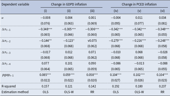
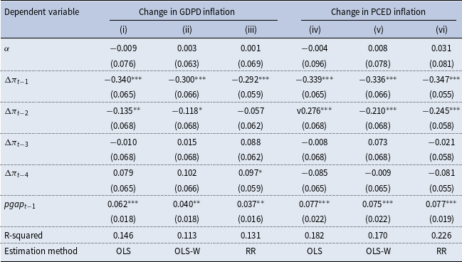
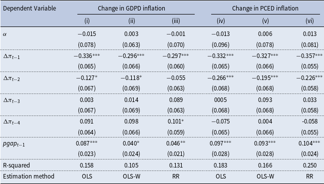
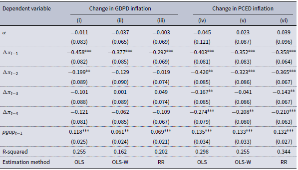
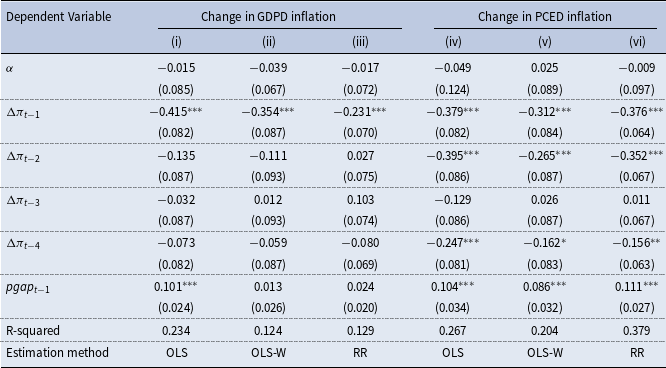
We initially estimate (1) using linear regression techniques. The Akaike Information Criterion points to including four lags of the dependent variables on the right-hand side of (1), while the Schwartz Bayesian Criterion selects two lags. The regression results are not sensitive between the two; here, we report those based on a lag length of four. Tables 1–3 report the estimation results with the price gap calculated in turn using each of the three Divisia money stocks. Each table panel has six columns of results with the first three concerning regressions where the change in the GDP deflator inflation series is the dependent variable and the remaining three those where the change in the PCE deflator inflation series is the regressand.
Linear estimations of (1) using DVM2 as the monetary aggregate

Table 1. Long description
The table presents regression results for the change in GDP deflator inflation and PCE deflator inflation using different estimation methods. The columns are labeled as follows: (i) Change in GDPD inflation, (ii) Change in GDPD inflation, (iii) Change in GDPD inflation, (iv) Change in PCED inflation, (v) Change in PCED inflation, and (vi) Change in PCED inflation. The rows are labeled with variables: alpha, Delta pi subscript t-1, Delta pi subscript t-2, Delta pi subscript t-3, Delta pi subscript t-4, pgap subscript t-1, R-squared, and Estimation method. Each cell contains numerical values and standard errors in parentheses. The table compares the impact of different lags of the dependent variable and the lagged price gap on inflation changes using Ordinary Least Squares (OLS), OLS with weights (OLS-W), and Recursive Residuals (RR) methods.
Notes: Sample period: 1967Q1–2024Q4. Standard errors in brackets. ***, **, * denote statistical significance at the one, five and ten percent levels, respectively. Columns (i–iii) use GDP data; columns (iv–vi) use PCE data.
Columns (i) and (iv) of Tables 1–3 report the regression results based on OLS estimation.Footnote 10 The lagged price gap coefficients in these columns are each significant at the one percent level with coefficient values in the range of 0.062 to 0.087 in the column (i) entries and 0.077 to 0.104 in column (iv).Footnote 11 These coefficient values are marginally lower than those reported in previous studies that employed OLS to estimate the P-star model. Hallman et al. (Reference Hallman, Porter and Small1991) report a coefficient value of 0.148 on a (simple-sum) M2-based price gap for a sample period covering 1955Q1 to 1988Q4 (as shown in a robustness test in Appendix 2, when we use that particular monetary aggregate, the price gap coefficient is 0.105).
Linear estimations of (1) using DVMZM as the monetary aggregate

Table 2. Long description
The table presents linear estimations of inflation changes using DVMZM as the monetary aggregate. The columns are labeled as follows: (i), (ii), (iii) under ‘Change in GDPD inflation’ and (iv), (v), (vi) under ‘Change in PCED inflation’. The rows include estimates of the constant term, lagged changes in inflation and the lagged price gap. Each cell contains numerical values with standard errors in brackets. The table also includes R-squared values and estimation methods (OLS, OLS-W, RR) indicated for each column. Asterisks indicate statistical significance at various levels.
Notes: Sample period: 1967Q1–2024Q4. Standard errors in brackets. ***, **, * denote statistical significance at the one, five and ten percent levels, respectively. Columns (i–iii) use GDP data; columns (iv–vi) use PCE data.
Linear estimations of (1) using DVM4 as the monetary aggregate

Notes: Sample period: 1967Q1–2024Q4. Standard errors in brackets. ***, **, * denote statistical significance at the one, five and ten percent levels, respectively. Columns (i–iii) use GDP data; columns (ivvvi) use PCE data.
Having confirmed the result of previous studies that the P-star model has explanatory power over changes in inflation on average, the other columns of Tables 1–3 use linear regression techniques that ameliorate the influence of outliers on linear coefficient estimates by down-weighting observations that can be considered outliers given the time series distribution of the variables. Columns (ii) and (v) of Tables 1–3 report the results of estimating (1) on a winsorised sample in which observations of each variable below the 10th percentile are replaced with values at that percentile and, likewise, those above the 90th percentile are replaced with values at that percentile. The price gap coefficients from these winsorised regressions (OLS-W) remain significant with a broadly unchanged coefficient in column (v) of each table, where consumption-related variables are under consideration, compared to column (iv). Coefficients in column (ii) of each table, where GDP and its deflator are of concern, are significant but lower than those in column (i). The results where a RR estimator is applied are shown in columns (iii) and (vi) of each table. This procedure involves removing the influence of outliers on coefficient estimates by down-weighting those observations in the regression in proportion to the size of their corresponding residuals, with results broadly comparable to those using the winsorised sample occurring. In summary, the regression results in Tables 1–3 indicate that price gaps have a positive and significant effect on inflation dynamics. This holds across different money stocks and the exclusion of episodes in which inflation is particularly high (and low).Footnote 12 – Footnote 14
3.2. Quantile regressions
Having undertaken linear analysis, we now move to reporting the results of estimating the P-star model using quantile regressions across a specified quantile range. While the influence of extreme values can be reduced through the use of linear techniques, such as those employed alongside OLS in the last sub-section, quantile regressions can capture the impact of outlying observations by modelling the full conditional distribution of the dependent variable. The quantile regressions here assess the impact of the price gap on the change-in-inflation variable across the conditional distribution of that inflation variable. The relationship between the two variables is no longer assumed to be linear and any variations in the significance and size of the coefficient on the price gap across the distribution can be ascertained. To assess whether any such variation arises, we consider the range of quantiles around the median from the 0.05 to the 0.95 quantiles.
A regression equation of the following form is estimated:
 \begin{align}{\unicode[Arial]{x0394}} {\pi }_{t}^{q}=\alpha +{\beta }_{1}^{q}{\unicode[Arial]{x0394}} \pi _{t-1}+{\beta }_{2}^{q}{\unicode[Arial]{x0394}} \pi _{t-2}+{\beta }_{3}^{q}{\unicode[Arial]{x0394}} \pi _{t-3}+{\beta }_{4}^{q}{\unicode[Arial]{x0394}} \pi _{t-4}+{\vartheta }_{t}^{q}pgap_{t-1}+{\varepsilon }_{t}^{q}\end{align}
Where all variables are defined as previously and the quantile values are denoted by the superscript
 $q$
(
 $q\in (0,1)$
).
The results of estimating (4), using each of the three price gaps derived using DVM2, DVMZM and DVM4, are shown in Figures 5 (where, analogous to the first three columns of Tables 1–3, GDP-based data are used) and 6 (where, as per the final three columns of those tables, consumption-based data are used). In the two rows of these figures, the constant and price gap coefficients are plotted as well as 90 and 95 percent error bands.Footnote
15
In the first row, the constant term, as one would expect to occur across the distribution of the dependent variable, rises steadily in value through the quantile range: from about −1.8 at the 0.05 quantile to close to two at the 0.95 quantile in Figure 5 and from about −2.1 at the 0.05 quantile to, again, close to two when
 $q$
equals 0.95 in Figure 6.
Quantile regression coefficients of (4)—dependent variable: change in GDPD inflation.
Note: The horizontal axis represents the quantile range; the vertical axis indicates the coefficient values. The thick black line indicates the coefficient value; the dark- and light-shaded areas are the 90 and 95 percent confidence bands, respectively.

Figure 5. Long description
The image contains three panels, each with two line graphs. Panel 1: The top graph shows the relationship between a constant and the quantile range, with the horizontal axis representing the quantile range from 0.05 to 0.95 and the vertical axis indicating coefficient values ranging from -2 to 3. The thick black line represents the coefficient value, with dark and light shaded areas indicating the 90 and 95 percent confidence bands, respectively. The bottom graph shows the price gap between DVM2 and GDP with the horizontal axis representing the quantile range from 0.05 to 0.95 and the vertical axis indicating values ranging from -0.05 to 0.2. The thick black line represents the price gap, with dark and light shaded areas indicating the 90 and 95 percent confidence bands, respectively. Panel 2: The top graph shows the relationship between a constant and the quantile range, with the horizontal axis representing the quantile range from 0.05 to 0.95 and the vertical axis indicating coefficient values ranging from -2 to 3. The thick black line represents the coefficient value, with dark and light shaded areas indicating the 90 and 95 percent confidence bands, respectively. The bottom graph shows the price gap between DVMZM and GDP with the horizontal axis representing the quantile range from 0.05 to 0.95 and the vertical axis indicating values ranging from -0.05 to 0.2. The thick black line represents the price gap, with dark and light shaded areas indicating the 90 and 95 percent confidence bands, respectively. Panel 3: The top row shows the relationship between the constant term and the quantile range, with the horizontal axis representing the quantile range from 0.05 to 0.95 and the vertical axis indicating coefficient values ranging from -2 to 3. The bottom row shows the price gap between DVM4 and GDP with the horizontal axis representing the quantile range from 0.05 to 0.95 and the vertical axis indicating values ranging from -0.05 to 0.2.
Quantile regression coefficients of (4)—dependent variable: change in PCED inflation.
Note: The horizontal axis represents the quantile range; the vertical axis indicates the coefficient values. The thick black line indicates the coefficient value; the dark- and light-shaded areas are the 90 and 95 percent confidence bands, respectively.

The estimated coefficients of the price gap in (4) are shown across the quantile range in the second row of Figure 5 and 6. There are differences between both figures according to the monetary aggregate and activity measure used. In Figure 5, where GDP is the activity variable, the DVM2 panel shows the (positive) price gap being significant from the 0.05 to 0.62 and 0.87 to 0.95 portions of the quantile range. The price gap coefficient has a marginally smaller quantile range of significance when DVMZM is the monetary aggregate used. It is much less significant when DVM4 is the basis for calculating the price gap. It is significant for quantile values from 0.05 to 0.37 and 0.86 to 0.95. In Figure 6, where consumption data are used in constructing the gaps and where the dependent variable is the change in PCE inflation, the gaps for all three monetary aggregates are significant over a much longer and continuous range, from
 $q$
values of 0.23 to 0.95.
Figure 6 and, to a lesser extent, Figure 5 then indicate the price gap having explanatory power for the change-in-inflation variable over most, or much, of the quantile range. In five of the six charts within those figures, the price gap is significant over some two-thirds or more of the quantile range and where consumption is used as the activity variable, it is significant for about 80 percent of the range. Thus, money developments, as captured in the price gap, can be assessed to impart a general inflationary response, one that is robust to the exclusion of outlier values (i.e., those in the tails of the change-in-inflation series’ distributions). While the coefficient of the price gap has a positive sign, its size, nevertheless, varies across the conditional distribution of inflation. In particular, the price gap has its largest coefficient values at the upper quantiles (the coefficients in Figure 6 tend to rise steadily over the quantile range, reaching their highest values at
 $q$
values of between 0.75 and 0.93). This indicates that adjustment to price equilibrium occurs more quickly in the upper quantiles than it does, for example, at the median (
 $q=0.5$
) value.Footnote
16
,
Footnote
17
It is worth restating though that the monetary impulse to inflation arises as a general phenomenon and not to those specific episodes highlighted by De Grauwe and Polan (Reference De Grauwe and Polan2005) and Borio et al. (Reference Borio, Hofmann and Zakrajšek2023a, Reference Borio, Lombardi, Yetman and Zakrajšek2023b).
4. Econometric results using the velocity gap and the output gap
4.1 Linear regressions
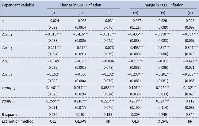
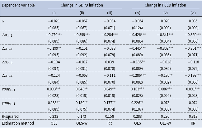
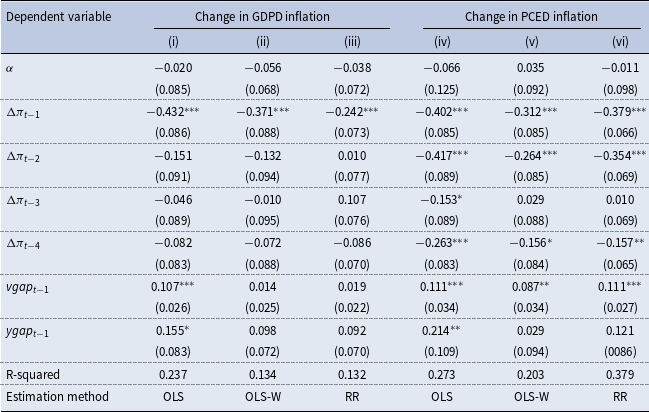
In this section, we substitute the velocity gap and output gap for the price gap, as per equation (3), and repeat the linear and quantile estimations of the previous section. The breakdown of the price gap into these two components not only follows algebraically from the construction of the price gap but also reflects the quantity-theoretic view that changes in the money stock are transmitted to inflation through two channels. Since changes in the money stock are not immediately transmitted to changes in the price level then both velocity (
 $V$
) and output (
 $Y$
) must deviate from their respective long run values,
 $V^{*}$
and
 $Y^{*}$
, until price equilibrium is restored. For example, an increase in the equilibrium price level caused by an rise in the money stock will lead the observed price level to rise to that new equilibrium value with a lag. During the adjustment period, the velocity of money will be expected to be below its equilibrium value and real output higher than its equilibrium level. The correction of those two variables over time to their equilibrium values will bring with it a higher price level.
Both channels of monetary transmission are acknowledged in the literature. The output channel has been highlighted frequently as a means of monetary transmission (see Humphrey, Reference Humphrey1989) with a short-lived rise in real spending occurring following an increase in the money stock. The velocity channel operates with the public’s holding of money rising in this case initially relative to income but the lagged, proportional rise in the price level relative to the change in the money stock dissipating those excess real balances over time. Decomposing the price gap into a velocity gap and an output gap can indicate the relative importance of each to the price adjustment process and, as per the focus here, whether one is stronger than the other at particular points of the statistical distribution of the inflation variable.
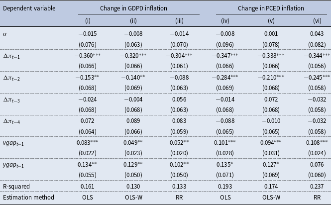
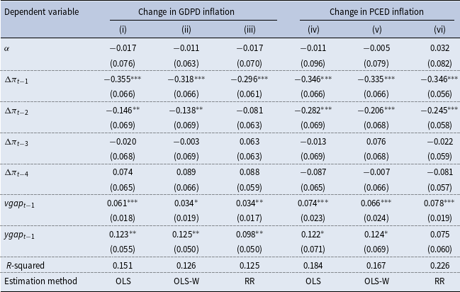
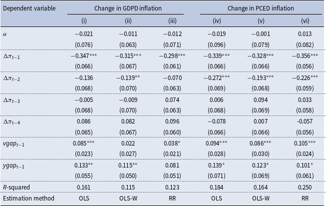
Tables 4–6 contain the results of the estimations of (3) using, again, alternative linear regression techniques and money stock-activity combinations.Footnote 18 As with the price-gap results reported in section 3, those estimations where the velocity and output gaps are calculated using personal consumption tend to be a better fit to the data, as indicated by the R-squared values in the tables. Both gaps have the expected positive value throughout. The velocity gap is significant in all tables bar column (ii) of Table 6. Its coefficient is lower in columns (ii) and (iii) of each table, where the sample is winsorised and where the regressions are estimated using robust methods, respectively. The coefficients in columns (v) and (vi) of the tables, where those techniques are also applied and where consumption is the activity measure used, have similar values to those in columns (iv). The output gap is usually significant in the tables but there are columns in each table where it is insignificant when RRs are used.Footnote 19
Linear estimations of (3) using DVM2 as the monetary aggregate

Notes: Sample period: 1967Q1–2024Q4. Standard errors in brackets. ***, **, * denote significance at the one, five and ten percent levels, respectively. Columns (i–iii) use GDP data; columns (iv–vi) use PCE data.
Linear estimations of (3) using DVMZM as the monetary aggregate

Table 5. Long description
The table presents linear estimations of GDP and PCE inflation using DVMZM as the monetary aggregate. It has 10 rows and 6 columns. The columns are labeled as follows: Dependent variable, Change in GDPD inflation (i), Change in GDPD inflation (ii), Change in GDPD inflation (iii), Change in PCED inflation (iv), Change in PCED inflation (v), and Change in PCED inflation (vi). The rows include various coefficients and their standard errors. Row 1: α, -0.017, -0.011, -0.017, -0.011, -0.005, 0.032. Row 2: Δπt-1, -0.355***, -0.318***, -0.296***, -0.346***, -0.335***, -0.346***. Row 3: Δπt-2, -0.146**, -0.138**, -0.081, -0.282***, -0.206***, -0.245***. Row 4: Δπt-3, -0.020, -0.003, 0.063, -0.013, 0.076, 0.022. Row 5: Δπt-4, 0.074, 0.089, 0.088, 0.087, -0.007, -0.081. Row 6: vgap_t-1, 0.061***, 0.034*, 0.034**, 0.074***, 0.066***, 0.078***. Row 7: ygap_t-1, 0.123**, 0.125**, 0.098**, 0.122*, 0.124*, 0.075. Row 8: R-squared, 0.151, 0.126, 0.125, 0.184, 0.167, 0.226. Row 9: Estimation method, OLS, OLS-W, RR, OLS, OLS-W, RR. The table includes standard errors in brackets and denotes significance at the one, five, and ten percent levels, respectively.
Notes: Sample period: 1967Q1–2024Q4. Standard errors in brackets. ***, **, * denote significance at the one, five and ten percent levels, respectively. Columns (i–iii) use GDP data; columns (iv–vi) use PCE data.
Linear estimations of (3) using DVM4 as the monetary aggregate

Notes: Sample period: 1967Q1–2024Q4. Standard errors in brackets. ***, **, * denote significance at the one, five and ten percent levels, respectively. Columns (i–iii) use GDP data; columns (iv–vi) use PCE data.
Quantile regression coefficients of (5)—dependent variable: change in GDPD inflation.
Note: The horizontal axis represents the quantile range; the vertical axis indicates the coefficient values. The thick black line indicates the coefficient value; the dark- and light-shaded areas are the 90 and 95 percent confidence bands, respectively.

Figure 7. Long description
The image contains six line graphs arranged in a 2x3 grid. Panel (i): The top left graph shows the velocity gap (DVM2, GDP) on the vertical axis against the GDP gap on the horizontal axis. The thick black line represents the coefficient value, with dark and light shaded areas indicating the 90 and 95 percent confidence bands, respectively. The horizontal axis ranges from 0.05 to 0.95, and the vertical axis ranges from -0.05 to 0.3. Panel (ii): The top middle graph shows the velocity gap (DVMZM, GDP) with similar axes and confidence bands. Panel (iii): The top right graph shows the velocity gap (DVM4, GDP) with similar axes and confidence bands. The bottom row of graphs repeats the same structure but for the GDP gap.
4.2 Quantile regressions
The quantile regression specification involving the velocity gap and output gap is given by:
 \begin{align}{\unicode[Arial]{x0394}} {\pi }_{t}^{q}=\alpha +{\beta }_{1}^{q}{\unicode[Arial]{x0394}} \pi _{t-1}+{\beta }_{2}^{q}{\unicode[Arial]{x0394}} \pi _{t-2}+{\beta }_{3}^{q}{\unicode[Arial]{x0394}} \pi _{t-3}+{\beta }_{4}^{q}{\unicode[Arial]{x0394}} \pi _{t-4}+{{\vartheta _{1}}}_{t}^{q}vgap_{t-1}+{{\vartheta _{2}}}_{t}^{q}ygap_{t-1}+{\varepsilon }_{t}^{q}\end{align}
Where
 ${\unicode[Arial]{x0394}} {\pi }_{t}^{q}$
is
 $q$
th quantile of the conditional distribution of inflation changes, and coefficients
 ${\beta }_{i}^{q}$
,
 ${{\vartheta _{1}}}_{t}^{q}$
, and
 ${{\vartheta _{1}}}_{t}^{q}$
capture, respectively, the impact of lag i of the dependent variable, the velocity gap and the output gap on
 ${\unicode[Arial]{x0394}} {\pi }_{t}^{q}$
at quantile
 $q$
.
Quantile regression coefficients of (5)—dependent variable: change in PCED inflation.
Note: The horizontal axis represents the quantile range; the vertical axis indicates the coefficient values. The thick black line indicates the coefficient value; the dark- and light-shaded areas are the 90 and 95 percent confidence bands, respectively.

Figure 8. Long description
The image contains six line graphs arranged in a 2x3 grid. Each graph has a horizontal axis labeled with a range from 0.05 to 0.95 and a vertical axis with different labels and ranges. Panel (i) shows two graphs: the top graph is labeled ‘Velocity gap (DVM2, PCE)t-1’ with a vertical axis ranging from -0.2 to 0.4, and the bottom graph is labeled ‘PCE gap t-1’ with a vertical axis ranging from -0.4 to 0.8. Panel (ii) shows two graphs: the top graph is labeled ‘Velocity gap (DVZM, PCE)t-1’ with a vertical axis ranging from -0.2 to 0.3, and the bottom graph is labeled ‘PCE gap t-1’ with a vertical axis ranging from -0.4 to 0.8. Panel (iii) shows two graphs: the top graph is labeled ‘Velocity gap (DVM4, PCE)t-1’ with a vertical axis ranging from -0.2 to 0.4, and the bottom graph is labeled ‘PCE gap t-1’ with a vertical axis ranging from -0.4 to 0.8. Each graph features a thick black line indicating the coefficient value, with dark- and light-shaded areas representing the 90 and 95 percent confidence bands, respectively. The graphs illustrate the relationship between velocity gaps and output gaps over time, showing trends and confidence intervals.
Estimates of that quantile regression are shown in Figures 7 (for the GDP-based data) and 8 (for the consumption-based data). The first row of charts in each figure provides the estimates of the velocity gap across the quantile range of 0.05–0.95 panels, while the second row shows those of the output gap. Estimates of the constant term have similar values to those in Figure 5 and 6 and are not shown here. In Figure 7, the velocity gap estimates have similar properties to the price gap in Figure 5, where GDP is also used as the activity variable. The velocity gap is significant throughout most of the quantile range where DVM2 provides the monetary aggregate, only being insignificant between
 $q$
values of 0.67–0.81. The DVMZM velocity gap is also significant over most of the quantile range, while that of DVM4 is significant between 0.05–0.24 and 0.81–0.95 of the quantile distribution. The output gap is only significant in Figure 7 in the lowest quarter or so of the quantile range.
Turning to Figure 8, where consumption is the activity variable, the velocity gap is significant for most
 $q$
values with insignificant coefficient values arising only below
 $q=0.33$
. The coefficients also tend to rise the larger is the
 $q$
value, although they do decline after 0.85 for the two narrow monetary aggregates. The coefficients on the consumption gap are generally insignificant in Figure 8 and only have explanatory power over changes in PCE inflation at the lowest quantile values.
Both the linear and quantile regressions using the velocity gap and output gap then point to the money channel being the stronger route through which monetary transmission to inflation takes place. This holds best for the two narrow monetary aggregates and where personal consumption provides the deflator and measure of economic activity.
5. Conclusion
The high inflation rates observed after the recent Covid-19 pandemic have rekindled interest in the extent to which money developments affect inflation, with commentators drawing attention to strong money growth during the pandemic preceding the pickup in inflation in 2021 and 2022, a feature also of other past high-inflation episodes. While some commentators, for example, Castañeda and Congdon (Reference Castañeda and Congdon2020) and King (Reference King2022), argue that recent developments demonstrate that “money matters” to inflation in general, others, such as Borio et al. (Reference Borio, Hofmann and Zakrajšek2023a, Reference Borio, Lombardi, Yetman and Zakrajšek2023b), take the view that a positive relationship between money growth and prices arises only when inflation is high. The increase in inflation in the 2020s also draws attention to the need to address challenges in modelling monetary behaviour, such as arises from instability in the demand for money, and to choose monetary aggregates best suited to understanding the money-inflation relationship.
Our contribution to this monetary literature is two-fold in nature. First, we advocate for, and illustrate, the use of quantitative techniques that account for the full conditional distribution of inflation as the basis for a richer understanding of the money-inflation relationship (without calling for a targeting of money aggregates by central banks in policymaking). Those techniques provide a means of extracting greater information about inflationary processes, whether the rate of change in the price level is moderate or high. Secondly, while the P-star literature has seen that model being developed and extended over time, this paper moves beyond the OLS estimation that has been employed in most of its applications. Taking account of recent studies that indicate the need to be attentive to measurement and other methodological issues, we use estimation procedures that mitigate the influence of outliers in linear estimations (OLS-W and RRs) and, separately, that investigate any asymmetries in the money-prices relationship to assess whether it holds only beyond certain inflation thresholds (quantile regressions).
While showing the impact of the price gap on the change in inflation being stronger at the upper end of the latter’s distribution, we demonstrate that a significant monetary impulse to prices occurs across most of the inflation variable’s range, running contrary to the contention that money only matters to price developments when inflation is high and that there is little connection between the two otherwise. The paper also finds the velocity gap having greater explanatory power over inflation than the output gap, pointing to the money channel being more important than the goods market channel in the transmission process. A stronger relationship is observed when consumption-based variables, rather than those based on GDP, are used in the econometric estimations. The 2020–22 episode of high inflation included observations that lie in the upper quartile of the distribution of inflation in our sample. The quantile regression analysis then indicates monetary factors having a particularly strong impact on general price developments during the pandemic and its aftermath. This supports the findings of Bordo and Duca (Reference Bordo and Duca2025), who argue that the type of monetary intervention employed during the pandemic can have a rapid impact on inflation such that it should be used rarely and on a temporary (short-lived) basis only.
In conclusion, the results reported here indicate the influence of money on inflation to be a general one and not owing to particular episodes of high inflation. Our analysis chimes with King’s (Reference King2022, p. 11) view that “we should say farewell … to the pretence that money has nothing to do with inflation” and that monetary variables matter to price developments in broader circumstances than many of those sympathetic to the “money matters” perspective acknowledge. In this regard, ongoing and innovative study of the money-inflation relationship should remain a critical focus of central banks and macroeconomic analysts more generally.
Acknowledgements
We acknowledge the very helpful comments of two anonymous referees and an associate editor.
Competing interests
No competing interests.
Appendix 1
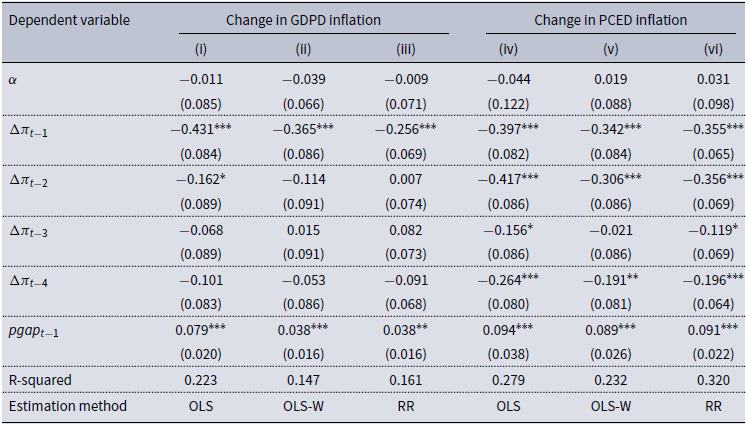
Linear estimations of (1) using DVM2 as the monetary aggregate

Notes: Sample period: 1990Q1-2024Q4. Standard errors in brackets. ***, **, * denote statistical significance at the one, five and ten percent levels, respectively. Columns (i)-(iii) use GDP data; columns (iv)-(vi) use PCE data.
Linear estimations of (1) using DVMZM as the monetary aggregate

Table A1b. Long description
The table presents regression results analyzing the impact of price gaps on inflation changes using different monetary aggregates and regression techniques. The rows are labeled with constant term and lagged coefficients. The columns are labeled with different regression methods and their effects on changes in GDPD inflation and PCED inflation. Each cell contains regression coefficients and standard errors. The table includes the following rows: alpha, Delta Pi sub t-1, Delta Pi sub t-2, Delta Pi sub t-3, Delta Pi sub t-4, pgap sub t-1, R-squared, and Estimation method. The columns are labeled as Change in GDPD inflation (i, ii, iii) and Change in PCED inflation (iv, v, vi). Each column provides coefficients and standard errors for different regression techniques: OLS, OLS-W, and RR. Notable trends include significant coefficients for lagged inflation terms and price gaps across different regression methods.
Notes: Sample period: 1990Q1-2024Q4. Standard errors in brackets. ***, **, * denote statistical significance at the one, five and ten percent levels, respectively. Columns (i)-(iii) use GDP data; columns (iv)-(vi) use PCE data.
Linear estimations of (1) using DVM4 as the monetary aggregate

Notes: Sample period: 1990Q1-2024Q4. Standard errors in brackets. ***, **, * denote statistical significance at the one, five and ten percent levels, respectively. Columns (i)-(iii) use GDP data; columns (iv)-(vi) use PCE data.
Linear estimations of (3) using DVM2 as the monetary aggregate

Table A2a. Long description
The table presents the results of estimations of a model using different linear regression techniques and money stock-activity combinations. The columns are labeled as follows: Dependent variable, Change in GDPD inflation (i), Change in GDPD inflation (ii), Change in GDPD inflation (iii), Change in PCED inflation (iv), Change in PCED inflation (v), and Change in PCED inflation (vi). The rows are labeled with different variables and their respective values. The table includes the following data: Row 1: α, -0.024, -0.068, -0.031, -0.067, 0.026, 0.045. Row 2: Δπt-1, -0.510, -0.416, -0.318, -0.436, -0.350, -0.354. Row 3: Δπt-2, -0.251, -0.172, -0.073, -0.458, -0.317, -0.361. Row 4: Δπt-3, -0.149, -0.035, -0.006, -0.199, -0.036, -0.142. Row 5: Δπt-4, -0.152, -0.080, -0.132, -0.298, -0.201, -0.207. Row 6: vgap t-1, 0.140, 0.074, 0.083, 0.146, 0.126, 0.132. Row 7: ygap t-1, 0.259, 0.210, 0.220, 0.281, 0.114, 0.112. Row 8: R-squared, 0.270, 0.192, 0.187, 0.309, 0.249, 0.344. Row 9: Estimation method, OLS, OLS-W, RR, OLS, OLS-W, RR. The table compares the impact of different variables on changes in GDP and PCE inflation using various estimation methods.
Notes: Sample period: 1990Q1–2024Q4. Standard errors in brackets. ***, **, * denote statistical significance at the one, five and ten percent levels, respectively. Columns (i)-(iii) use GDP data; columns (iv)-(vi) use PCE data.
Linear estimations of (3) using DVMZM as the monetary aggregate

Notes: Sample period: 1990Q1–2024Q4. Standard errors in brackets. ***, **, * denote statistical significance at the one, five and ten percent levels, respectively. Columns (i)-(iii) use GDP data; columns (iv)-(vi) use PCE data.
Linear estimations of (3) using DVM4 as the monetary aggregate

Notes: Sample period: 1990Q1–2024Q4. Standard errors in brackets. ***, **, * denote statistical significance at the one, five and ten percent levels, respectively. Columns (i)-(iii) use GDP data; columns (iv)-(vi) use PCE data.
Appendix 2
Linear estimations of (1) using DVM2 and M2 as the monetary aggregate

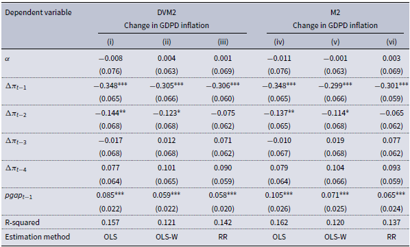
Table A3a. Long description
The table presents linear estimations of GDP inflation using DVM2 and M2 as monetary aggregates. It has six columns and seven rows, including headers and footnotes. The columns are labeled as (i), (ii), (iii) for DVM2 and (iv), (v), (vi) for M2, each representing different estimation methods. The rows include variables such as alpha, Delta Pi sub t-1, Delta Pi sub t-2, Delta Pi sub t-3, Delta Pi sub t-4, pgap sub t-1, R-squared, and Estimation method. Each cell contains numerical values with standard errors in brackets. Notable trends include significant values for Delta Pi sub t-1 and pgap sub t-1 across all columns, indicating their strong influence on GDP inflation. The R-squared values vary slightly across different estimation methods, reflecting the model’s explanatory power.
Notes: Sample period: 1967Q1-2024Q4. Standard errors in brackets. ***, **, * denote statistical significance at the one, five and ten percent levels, respectively. The entries in columns (i) to (iii) are those in columns (i) to (iii) of Table 1, where DVM2 is used, while those in columns (iv) to (vi) use M2 as the monetary aggregate.
Appendix 3
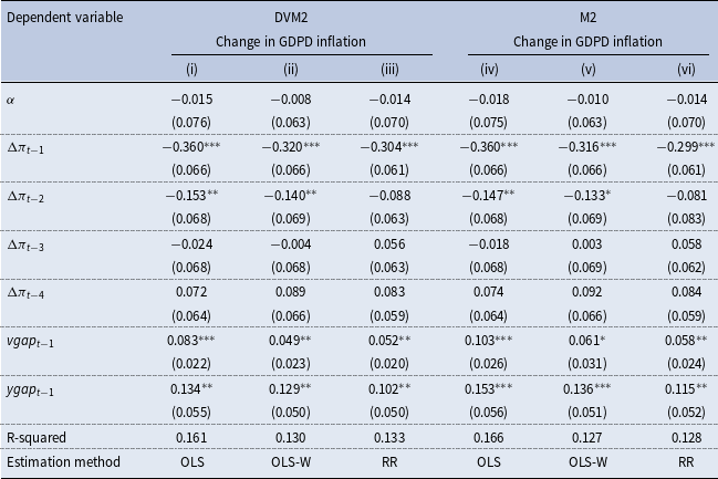
Linear estimations of (3) using DVM2 and M2 as the monetary aggregate

Notes: Sample period: 1967Q1-2024Q4. Standard errors in brackets. ***, **, * denote statistical significance at the one, five and ten percent levels, respectively. The entries in columns (i) to (iii) are those in columns (i) to (iii) of Table 4, where DVM2 is used, while those in columns (iv) to (vi) used M2 as the monetary aggregate.
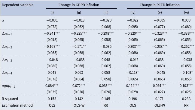
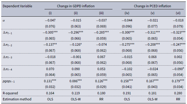
Linear estimations of (1) using DVM2 and Local Linear Trends

Table A5a. Long description
The table presents linear estimations of changes in GDP deflation and PCE deflation using different methods. It has six columns and eight rows, including headers and notes. The columns are labeled as follows: (i), (ii), (iii) for changes in GDP deflation and (iv), (v), (vi) for changes in PCE deflation. The rows include the following variables and values: Row 1: α, -0.031, -0.013, -0.029, -0.022, -0.005, 0.003. Row 2: Δπt-1, -0.341***, -0.325***, -0.298***, -0.329***, -0.328***, -0.338***. Row 3: Δπt-2, -0.169***, -0.171**, -0.095, -0.303***, -0.233***, -0.262***. Row 4: Δπt-3, -0.048, -0.038, 0.048, -0.042, 0.038, 0.038. Row 5: Δπt-4, 0.049, 0.063, 0.058, -0.118*, -0.045, -0.108*. Row 6: pgapt-1, 0.084***, 0.072***, 0.063***, 0.114***, 0.094***, 0.103***. Row 7: R-squared, 0.153, 0.142, 0.145, 0.196, 0.171, 0.233. Row 8: Estimation method, OLS, OLS-W, RR, OLS, OLS-W, RR. The table includes standard errors in brackets and denotes statistical significance at the one, five, and ten percent levels, respectively.
Notes: Sample period: 1967Q1-2024Q4. Standard errors in brackets. ***, **, * denote statistical significance at the one, five and ten percent levels, respectively. Columns (i)-(iii) use GDP data; columns (iv)-(vi) use PCE data.
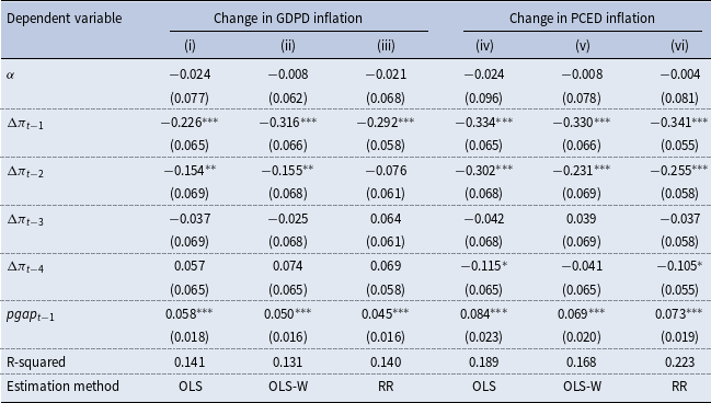
Linear estimations of (1) using DVMZM with Local Linear Trends

Notes: Sample period: 1967Q1-2024Q4. Standard errors in brackets. ***, **, * denote statistical significance at the one, five and ten percent levels, respectively. Columns (i)-(iii) use GDP data; columns (iv)-(vi) use PCE data.
Linear estimations of (1) using DVM4 with Local Linear Trends

Table A5c. Long description
The table presents linear estimations of changes in GDP deflator inflation and PCE deflator inflation using different estimation methods. It has 10 rows and 6 columns. The columns are labeled as follows: (i) Change in GDPD inflation, (ii) Change in GDPD inflation, (iii) Change in GDPD inflation, (iv) Change in PCED inflation, (v) Change in PCED inflation, (vi) Change in PCED inflation. The rows are labeled with variables and their respective values. Row 1: α, -0.047, -0.015, -0.037, -0.044, -0.021, -0.018. Row 2: Δπt-1, -0.305***, -0.296***, -0.285***, -0.300***, -0.311***, -0.323***. Row 3: Δπt-2, -0.137**, -0.126*, -0.074, -0.275***, -0.208***, -0.247***. Row 4: Δπt-3, -0.018, -0.001, 0.067, -0.015, 0.068, 0.002. Row 5: Δπt-4, 0.070, 0.090, 0.053, -0.102, -0.024, -0.090*. Row 6: pgapt-1, 0.131***, 0.086***, 0.126***, 0.158***, 0.167***, 0.179***. Row 7: R-squared, 0.164, 0.119, 0.180, 0.191, 0.181, 0.280. Row 8: Estimation method, OLS, OLS-W, RR, OLS, OLS-W, RR. The table includes standard errors in brackets and denotes statistical significance at the one, five, and ten percent levels, respectively.
Notes: Sample period: 1967Q1–2024Q4. Standard errors in brackets. ***, **, * denote statistical significance at the one, five and ten percent levels, respectively. Columns (i)-(iii) use GDP data; columns (iv)-(vi) use PCE data.
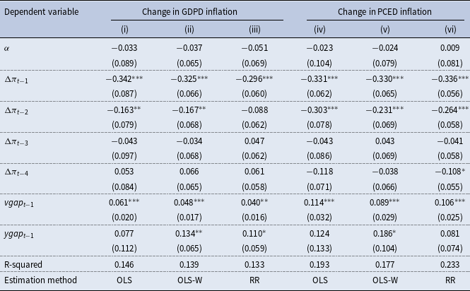
Linear estimations of (3) using DVM2 with Local Linear Trends

Notes: Sample period: 1967Q1–2024Q4. Standard errors in brackets. ***, **, * denote significance at the one, five and ten percent levels, respectively. Columns (i) to (iii) use GDP data; columns (iv) to (vi) use PCE data.
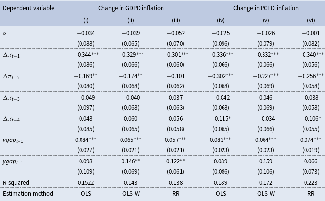
Linear estimations of (3) using DVMZM with Local Linear Trends

Table A6b. Long description
The table presents linear estimations of GDP and PCE inflation using different methods. It has 11 rows and 6 columns. The columns are labeled as follows: (i), (ii), (iii) for Change in GDPD inflation and (iv), (v), (vi) for Change in PCED inflation. The rows are labeled with different variables and their respective values. Row 1: α, -0.034, -0.039, -0.052, -0.025, -0.026, -0.001. Row 2: Δπt-1, -0.344***, -0.329***, -0.301***, -0.336***, -0.332***, -0.340***. Row 3: Δπt-2, -0.169**, -0.174**, -0.101, -0.302***, -0.227***, -0.256***. Row 4: Δπt-3, -0.049, -0.040, 0.037, -0.042, 0.046, -0.038. Row 5: Δπt-4, 0.048, 0.060, 0.056, -0.115*, 0.034, -0.106*. Row 6: vgap_t-1, 0.084***, 0.065***, 0.057***, 0.083***, 0.064***, 0.074***. Row 7: ygap_t-1, 0.098, 0.146**, 0.122**, 0.089, 0.159, 0.066. Row 8: R-squared, 0.1522, 0.143, 0.138, 0.189, 0.172, 0.223. Row 9: Estimation method, OLS, OLS-W, RR, OLS, OLS-W, RR. The table includes standard errors in brackets and denotes significance at the one, five, and ten percent levels, respectively.
Notes: Sample period: 1967Q1–2024Q4. Standard errors in brackets. ***, **, * denote significance at the one, five and ten percent levels, respectively. Columns (i) to (iii) use GDP data; columns (iv) to (vi) use PCE data.
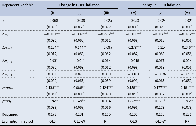
Linear estimations of (3) using DVM4 with local linear trends

Notes: Sample period: 1967Q1–2024Q4. Standard errors in brackets. ***, **, * denote significance at the one, five and ten percent levels, respectively. Columns (i) to (iii) use GDP data; columns (iv) to (vi) use PCE data.