





1. Introduction
Porous membranes are solid structures perforated by a matrix of pores, which allow a fluid to flow through this matrix. The pores may be in the nanometre range or even smaller, thus challenging traditional fluid flow models based on the continuum mechanics assumption. For example, cell membranes of plants and animals are crossed by sub-nanometric channels dedicated to specific functions, such as aquaporins (Agre et al. Reference Agre, Preston, Smith, Jung, Raina, Moon, Guggino and Nielsen1993) and ion channels (Alberts et al. Reference Alberts, Bray, Hopkin, Johnson, Lewis, Raff, Roberts and Walter2014). Filtration systems, used in the oil and medical industries, desalination plants and other environmental applications, are often characterised by the presence of porous membranes (Mohanty & Purkait Reference Mohanty and Purkait2011), and the range of typical sizes of these structures is very wide. For example, reverse-osmosis membrane filters have pores in the nanometric range (Greenlee et al. Reference Greenlee, Lawler, Freeman, Marrot and Moulin2009), while the membrane assembly’s typical length is in the order of metres. Among these manmade structures, membranes based on carbon nanotubes (CNTs) have recently attracted attention in the fluid dynamics community because of their ability to transport water efficiently (Jue et al. Reference Jue, Buchsbaum, Chen, Park, Meshot, Wu and Fornasiero2020). These membranes have pore radii in the nanometric range, and can be grown very long to constitute fibres (Huang et al. Reference Huang, Zhang and Liu2020), or alternatively, shorter nanotubes can be packed together to form a thin porous sheet (Lee et al. Reference Lee, Jeong and Liu2016).
In the case of membranes whose typical pore size is such that continuum equations are valid, one approach is to perform full-scale calculations of the flow across whole membrane systems: e.g. Falcucci et al. (Reference Falcucci, Amati, Fanelli, Krastev, Polverino, Porfiri and Succi2021, Reference Falcucci, Polverino, Porfiri, Amati, Fanelli, Krastev and Succi2022, Reference Falcucci, Amati, Bella, Facci, Krastev, Polverino, Succi and Porfiri2024) for the sponge Euplectella aspergillum, and Wang et al. (Reference Wang, Mukherjee and Wang2006) for a polymer-electrolyte fuel cell. However, for nanometric and sub-nanometric systems, such simulations are possible only for limited membrane portions and time ranges, using molecular dynamics (MD) simulations. For example, Frallicciardi et al. (Reference Frallicciardi, Melcr, Siginou, Marrink and Poolman2022) computed the permeability of a lipid membrane whose side is approximately
 $10\ \text{nm}$
to various weak acids and glycerol, while Pezeshkian et al. (Reference Pezeshkian, König, Wassenaar and Marrink2020) performed a very large simulation (
 $83$
million particles) of a full mitochondrial membrane. Despite their accuracy and increasing computational power due to heavily parallelised algorithms, MD simulations remain prohibitively expensive. For this reason, some authors such as Gravelle et al. (Reference Gravelle, Joly, Detcheverry, Ybert, Cottin-Bizonne and Bocquet2013) explored simplified pore-scale descriptions based on Stokes equations with ad hoc conditions on the pore walls to reproduce the flow rates found via MD simulations. The application of continuum mechanics to such systems is certainly questionable, and the state-of-the-art tool for these structures remains the MD framework (Gubbiotti et al. Reference Gubbiotti, Baldelli, Muccio, Malgaretti, Marbach and Chinappi2022).
In this area, we find several types of computational strategies to account for the dynamics of molecules through nanopores. For example, ab initio computations can account for quantum-mechanical processes, but have prohibitive computational costs, whereas simulations based on empirical force fields apply to much larger systems and longer times. In the latter, atoms are modelled as material points subject to Newton’s law of motion. The mutual forces exchanged between these material points are rendered by potentials, which depend on the nature of the interaction (bonded or non-bonded), the distance between the two material points, and their atom type. Integrating numerically in time the law of motion of these material points, we find their trajectories. Despite being cheaper than ab initio simulations, these computations are still costly compared to continuum-mechanics models (Allen & Tildesley Reference Allen and Tildesley1989). A third approach, with slightly lighter computational cost, consists of coarse-grained models, where clusters of fluid molecules are considered as a single particle with effective properties. These approaches involve a higher level of modelling and can match hydrodynamics close to solid–liquid interfaces (Cambiaso et al. Reference Cambiaso, Tagliabue, Bochicchio, Tinti, Rasera, Giacomello, Monticelli and Rossi2025). Coarse-grained techniques, however, have a computational cost orders of magnitude larger than the classical continuum approach based on the solution of Navier–Stokes equations. Real nanoporous membrane systems are formed by thousands of pores over a metre scale, and the simulation of such systems is computationally challenging also with a full continuum approach.
In such an overall picture, average models provide a convenient alternative (Brennan et al. Reference Brennan, Yeo, Pearce and Dalwadi2026). They consist of simplified (macroscopic) flow descriptions that account only for the average effect of the membrane on the fluid flow. A set of coefficients, appearing in the membrane-scale equations, models the effect of the pore geometry on the macroscopic flow. Darcy (Reference Darcy1856) was the first to propose such a description for bulk porous media, experimentally deducing a linear relationship between the pressure gradient and the flow rate for a water stream across a sand column. Thus the factor expressing this proportionality, i.e. the permeability coefficient, was found empirically. On the other hand, Sampson (Reference Sampson1891) analytically computed the flow rate across an infinitesimally thin membrane with a central, isolated pore, finding a cubic dependence of the flow rate on the pore radius without employing empirical coefficients. More recently, Tio & Sadhal (Reference Tio and Sadhal1994) and Jensen et al. (Reference Jensen, Valente and Stone2014) generalised the Sampson model, including inter-pore interactions, inertia and confinement, via semi-empirical coefficients. However, they considered an idealised set-up, consisting of a fluid flow purely perpendicular to the membrane. Generalising such models to arbitrary pore geometries and flow conditions is difficult because they lack a direct, explicit link between the pore geometry and the coefficients representing them. Thanks to multi-scale homogenisation (Mei & Vernescu Reference Mei and Vernescu2010), Zampogna & Gallaire (Reference Zampogna and Gallaire2020) and Zampogna et al. (Reference Zampogna, Ledda, Wittkowski and Gallaire2023) proposed to interpret these coefficients, called Navier tensors, as the solution to a set of Stokes problems solved in a periodic control volume containing the pore geometry. In their model, they considered inertialess, single-phase flow at the pore scale.
However, these models rely on the applicability of continuum mechanics at the pore scale; when pore sizes reach the nanometric or sub-nanometric range, this assumption may no longer be valid, and the models may lose predictive accuracy. For example, Cheng & Giordano (Reference Cheng and Giordano2002) experimentally measured the flow rate across channels in the micrometres and tens-of-nanometres range, finding that for some fluids, such as hexadecane, the flow rate predicted using Poiseuille’s law and no-slip at the walls is approximately six times smaller than the experimental flow rate. They suggest that these substances slip along the solid walls. The correct flow rate can be then retrieved using the wall slip as a fitting parameter, which leads to a modification of the classic Poiseuille profile. However, they did not observe such behaviour for water. Gravelle et al. (Reference Gravelle, Joly, Detcheverry, Ybert, Cottin-Bizonne and Bocquet2013, Reference Gravelle, Joly, Ybert and Bocquet2014) pointed out that in the case of water across aquaporins, there is a good agreement between the hydrodynamic and MD simulations, provided that the Stokes equations are used with a slip condition for the flow velocity at the pore walls. On the other hand, Thiemann et al. (Reference Thiemann, Schran, Rowe, Müller and Michaelides2022) simulated water flow across CNTs using machine-learning-aided MD, and found very small, radius-dependent, friction coefficients. He ascribed this slip behaviour to the interaction between the water’s oxygen and the carbon atoms in the nanotube. Secchi et al. (Reference Secchi, Marbach, Niguès, Stein, Siria and Bocquet2016) found that water passes through CNTs in a nearly frictionless regime. These few examples show how a single substance, such as water, can produce very different behaviours depending on the wall molecules at nanometric scales. Accounting for such a variety of phenomena in a continuum model is certainly a complex task, and MD simulations remain the state of the art for computing fluid flows at these scales. However, when we consider the fluid flow far from an interface (the pore walls in the present case), the validity of continuum mechanics is restored, and we are allowed to use continuous models such as the Navier–Stokes equations.
Attempts to couple the computational convenience of solving the Navier–Stokes equations with the accuracy of MD simulations are not new to the literature. For example, Ichikawa et al. (Reference Ichikawa, Kawamura, Fujii and Nattavut2002) coupled homogenisation with MD simulation to predict the diffusion of tritium and other substances across bentonite clay, an inhomogeneous material used in the containment of hazardous compounds, such as radioactive waste. Using homogenisation, Lund et al. (Reference Lund, Zhang, Mahelona and Hendy2012) calculated the slip length of chemically heterogeneous surfaces, and Pace et al. (Reference Pace, Rahmaninejad, Sun and Kekenes-Huskey2021) modelled the diffusion of aqueous methane across a silica matrix.
Often, upscaling methodologies are adapted to the particular flow situation and the involved materials to provide their macroscopic representation in terms of average effect. However, it would be interesting to explore the opposite, i.e how we can translate an existing homogenisation methodology in terms of MD simulations, to find a convenient way to treat a variety of problems at the nanometric level rather than tackling a single, specific problem, and adapting the methodology to it. For example, O’Connell & Thompson (Reference O’Connell and Thompson1995) proposed a hybrid method combining MD and Navier–Stokes equations to solve generic unidirectional fluid flows. They exploited the presence of an overlap region to avoid the problem of introducing the effect of different mean stresses at each location on the membrane. However, in the absence of inertia, the convenient decomposition of the microscopic fluid flow introduced by Zampogna et al. (Reference Zampogna, Ledda, Wittkowski and Gallaire2023) allows us to obtain from a single pore-scale solution the mean coefficients representing its macroscopic effect. Using MD to provide these coefficients from an accurate pore-scale solution is the key idea underlying this paper.
Thus we explore the possibility of coupling the accuracy of MD simulations at the pore scales with the convenient computational cost of numerically solving the Navier–Stokes equations far from the membrane. This approach applies the homogenisation method proposed by Zampogna et al. (Reference Zampogna, Ledda, Wittkowski and Gallaire2023) for thin membranes to upscale the effect of the pore geometry on the fluid flow in the outer region far from the membrane, by substituting the pore-scale continuum approach with an MD-based description.
In § 2.1, we briefly summarise the effective stress jump model developed by Zampogna et al. (Reference Zampogna, Ledda, Wittkowski and Gallaire2023), and in § 2.3, we introduce a strategy to translate the continuum pore-scale flow into the MD framework. In § 3, we consider a specific pore geometry, that of a single-wall armchair CNT, and compare MD and continuum-based results. In § 4, we consider a full membrane geometry and solve the flow across it using MD, and compare this solution with that of our homogeneous model, in which the membrane properties are computed using MD simulations. We summarise our results and discuss future perspectives in § 5.
2. Methodology
Multi-scale homogenisation methods (Mei & Vernescu Reference Mei and Vernescu2010) are developed under the hypothesis that the fluid flow admits a continuous description. However, the continuum assumption inside nanometric and sub-nanometric pores is certainly questionable; indeed, the size of the pore is only a few times larger than the size of the molecules. We aim to link the pore properties with the macroscopic flow far from the membrane, where the continuum description applies. To perform this operation, we consider the methodology developed by Zampogna et al. (Reference Zampogna, Ledda, Wittkowski and Gallaire2023), and use MD to obtain an accurate description of the effective pore-scale properties. In the next section, we summarise this methodology in the case of a purely continuum-based flow description.
2.1. The effective stress jump model for thin porous membranes
(a) Full-scale membrane as it appears in the physical world; the coordinate system is denoted by
 $(\hat {x}_1,\hat {x}_2,\hat {x}_3)$
. (b) Zoom in on the microscopic elementary cell. The fluid domain is denoted by
 $\mathbb{F}$
, and the upward and downward sides of the fluid domain by
 $\mathbb{U}$
and
 $\mathbb{D}$
, respectively. In the novel MD-homogenisation framework introduced in this work, the fluid flow within the microscopic elementary cell is provided by MD simulations. (c) Membrane mid-surface, which corresponds to the effective interface used to model the macroscopic effect of the porous microstructure.

Figure 1. Long description
Panel A: A diagram of a full-scale membrane with a coordinate system denoted by x1, x2, and x3. The membrane has a length L and a pore scale denoted by the symbol with a line through it. Panel B: A zoomed-in view of a microscopic elementary cell within the membrane. The fluid domain is denoted by F, and the upward and downward sides of the fluid domain are denoted by U and D, respectively. The cell has dimensions denoted by xn, xt, and xs. The fluid flow within the microscopic elementary cell is provided by molecular dynamics simulations. Panel C: A diagram of the membrane mid-surface, which corresponds to the effective interface used to model the macroscopic effect of the porous microstructure. The mid-surface is described using the Navier-Stokes equations, with interface conditions denoted by C and C+. The interface conditions are determined using molecular dynamics-aided homogenization.
We consider the incompressible flow of a Newtonian fluid characterised by constant density
 $\rho$
and viscosity
 $\mu$
crossing a thin, periodically microstructured, permeable membrane, as illustrated in figure 1(
 $a$
).
We represent the (dimensional) global coordinate system using
 $\hat {x}_i$
, and denote the dimensional fluid flow velocity and pressure as
 $\hat {u}_i$
and
 $\hat {p}$
, respectively, alongside
 $\hat {\tau }$
representing the dimensional time. Additionally, we introduce the inward-pointing normal and tangent vectors applicable to any boundary, denoted as
 $(\hat {\boldsymbol{n}},\hat {\boldsymbol{t}},\hat {\boldsymbol{s}})$
. Locally, at the surface, we can identify a periodic unit cell (i.e. a control volume that repeats at constant spacing along the membrane), and establish a dimensional local reference frame
 $(\hat {x}_n,\hat {x}_t,\hat {x}_s)$
. Assuming that the membrane curvature is negligible at the pore scale, the local frame of reference
 $(\hat {x}_n,\hat {x}_t,\hat {x}_s)$
is aligned with the normal and two tangent vectors
 $(\hat {\boldsymbol{n}},\hat {\boldsymbol{t}},\hat {\boldsymbol{s}})$
of the membrane centreline
 $\mathbb{C}$
at any point.
We focus on the periodic unit cell; see figure 1(b). We denote the fluid region inside it by
 $\mathbb{F}$
, the solid region by
 $\mathbb{M}$
, and the solid–fluid boundary by
 $\partial \mathbb{M}$
. We call
 $\mathbb{U}$
and
 $\mathbb{D}$
the upward and downward sides of
 $\mathbb{F}$
, respectively. The Navier–Stokes equations govern the evolution of the dimensional flow velocity
 $\hat {u}_i$
and pressure
 $\hat {p}$
in the whole fluid domain:
 \begin{equation} \begin{cases} \rho (\hat {\partial }_{\tau }\hat {u}_i+\hat {u}_{\!j}\,\hat {\partial }_{\!j} \hat {u}_i)=-\hat {\partial }_i \hat {p}+\mu\, \hat {\partial }_{kk}^2 \hat {u}_i, \\[11pt] \hat {\partial }_i \hat {u}_i=0, \\[11pt] \dfrac {\ell }{\mu }\chi _{\!j}\hat {\varSigma }_{ij}=\varphi _{ij} \hat {u}_{\!j} \quad \text{on } \quad \partial \mathbb{M}, \end{cases} \end{equation}
where we adopt Einstein’s convention that repeated indices are summed. In (2.1)
 $\hat {\varSigma }_{ij}=-\hat {p}\delta _{ij}+ ({1}/{2}) (\hat {\partial }_i\hat {u}_{\!j}+\hat {\partial }_{\!j}\hat {u}_i )$
represents the fluid stresses, and
 $\chi _{\!j}$
and
 $\varphi _{ij}$
contain non-dimensional coefficients that allow us to impose a variety of boundary conditions on the membrane; e.g. if
 $\chi _{\!j}=n_i$
and
 $\varphi _{ij}=0$
, then we have a full-slip condition (i.e. no shear at the wall and no-penetration), while if
 $\chi _{\!j}=0$
and
 $\varphi _{ij}=\delta _{ij}$
, then we have a no-slip condition. The separation of scales between the size of the unit cell
 $\ell$
and the size of the membrane
 $L$
suggests that we can study the fluid flow across the porous membrane by utilising a multi-scale technique. We denote with
 $\epsilon =\ell /L\ll 1$
the corresponding scale-separation parameter.
Homogenisation and matched asymptotic expansions enable the macroscopically equivalent model for the flow at the membrane, intended as an infinitely thin interface between two fluid domains (see figure 1(c), where the interface is denoted with
 $\mathbb{C}$
).
It is useful from now on to specify the typical flow scales in the vicinity of the membrane pores that are used in the homogenisation procedure to develop the macroscopic equations. These scales will be used afterwards to establish a direct link between the microscopic continuum and MD-based problems The viscous stresses must balance the pressure gradient in the near-pore region. The following normalisation holds:
 \begin{equation} \hat {x}_i=\ell x_i, \quad \hat {p}=\Delta P \ p=\frac {\mu U}{\ell }p, \quad \hat {u}_i=Uu_i, \quad \hat {\tau }=T\tau =\frac {\ell }{U}\tau, \end{equation}
where
 $U$
and
 $\Delta P$
are the pore-scale velocity and pressure scales, respectively. The characteristic scales introduced in (2.2) allow the definition of the microscopic Reynolds number as
 \begin{equation} \textit{Re}_\ell =\frac {\rho U \ell }{\mu }. \end{equation}
Normalising (2.1) using (2.2), we obtain
 \begin{equation} \begin{cases} \textit{Re}_\ell\, ({\partial }_{\tau }{u}_i+{u}_{\!j}\,{\partial }_{\!j} {u}_i)=-{\partial }_i {p}+ {\partial }_{kk}^2 {u}_i, \\[9pt] {\partial }_i {u}_i=0, \\[9pt] \chi _{\!j}{\varSigma }_{ij}=\varphi _{ij} {u}_{\!j} \quad \text{on } \quad \partial \mathbb{M}. \end{cases} \end{equation}
After applying homogenisation to system (2.4), we deduce the macroscopic equations governing the velocity and pressure field at the membrane
 $\mathbb{C}$
in the
 $\textit{Re}_\ell =0$
limit:
 \begin{align} {u}_i|_{\mathbb{C}^-}=\mathcal{M}^{-}_{ij}\varSigma _{jk}^{\mathbb{C}^-}n_k+\mathcal{N}^{-}_{ij}\varSigma _{jk}^{\mathbb{C}^+}n_k, \\[-12pt]\nonumber \end{align}
 \begin{align} {u}_i|_{\mathbb{C}^+}=\mathcal{M}^{+}_{ij}\varSigma _{jk}^{\mathbb{C}^-}n_k+\mathcal{N}^{+}_{ij}\varSigma _{jk}^{\mathbb{C}^+}n_k, \\[-12pt]\nonumber \end{align}
 \begin{align} {p}|_{\mathbb{C}^-}=\mathcal{Q}^{\mathbb{U}}_{\!j}\varSigma _{jk}^{\mathbb{C}^-}n_k+\mathcal{R}^{\mathbb{U}}_{\!j}\varSigma _{jk}^{\mathbb{C}^+}n_k, \\[-12pt]\nonumber \end{align}
 \begin{align} {p}|_{\mathbb{C}^+}=\mathcal{Q}^{\mathbb{D}}_{\!j}\varSigma _{jk}^{\mathbb{C}^-}n_k+\mathcal{R}^{\mathbb{D}}_{\!j}\varSigma _{jk}^{\mathbb{C}^+}n_k, \end{align}
where
 $\varSigma _{jk}^{\mathbb{C}^\pm }$
are the macroscopic fluid stresses computed on
 $\mathbb{C}^-$
and
 $\mathbb{C}^+$
, and the so-far unknown quantities
 $\mathcal{M}_{ij}^{\pm },\mathcal{N}_{ij}^{\pm }$
(Navier tensors) and
 $\mathcal{Q}_{\!j}^{\pm }$
and
 $\mathcal{R}_{\!j}^{\pm }$
(auxiliary pressures) are obtained by computing the solution of a set of solvability conditions, the so-called microscopic problems, averaged using the definitions
 \begin{equation} \overline {{\cdot }}^{-}_{} =\frac {1}{|\mathbb{U}|}\int _{\mathbb{U}}{\cdot }\,\text{d}t\, \text{d}s, \quad \overline {{\cdot }}^{+} =\frac {1}{|\mathbb{D}|}\int _{\mathbb{D}}{\cdot }\,\text{d}t\, \text{d}s, \end{equation}
 \begin{equation} \mathcal{M}_{ijk}^{-}=\overline {M}_{ijk}^{^-}-x_n\vert _{\mathbb{U}}(\delta _{it}\delta _{jt}+\delta _{is}\delta _{js})\delta _{kn}, \quad \mathcal{M}_{ijk}^{+}=\overline {{M}}_{ijk}^{^+}, \quad {\mathcal{Q}^\pm _{ij}=\overline {Q}^\pm _{ij},} \end{equation}
 \begin{equation} \mathcal{N}_{ijk}^{-}=\overline {{N}}_{ijk}^{^-}, \quad \mathcal{N}_{ijk}^{+}=\overline {N}_{ijk}^{^+}-x_n\vert _{\mathbb{D}}(\delta _{it}\delta _{jt}+\delta _{is}\delta _{js})\delta _{kn},\quad {\mathcal{R}^\pm _{ij}=\overline {R}^\pm _{ij},} \end{equation}
where
 $x_n\vert _{\mathbb{U}}$
and
 $x_n\vert _{\mathbb{D}}$
are the distances between
 $\mathbb{U}$
and the plane tangent to
 $\partial \mathbb{M}$
towards
 $\mathbb{U}$
and between
 $\mathbb{D}$
and the plane tangent to
 $\partial \mathbb{M}$
towards
 $\mathbb{D}$
, respectively. The microscopic problems read
 \begin{equation} \begin{cases} -\partial _i Q_{\!j} +\partial ^2_{hh}M_{ij}=0 \quad \text{in} \quad \mathbb{F},\\[9pt] \partial _i M_{ij}=0 \quad \text{in} \quad \mathbb{F},\\[9pt] \varSigma _{hq}(M_{\boldsymbol{\cdot }j},Q_{\!j})n_q=\delta _{jh} \quad \text{on} \quad \mathbb{U},\\[9pt] \varSigma _{hq}(M_{\boldsymbol{\cdot }j},Q_{\!j})n_q=0 \quad \text{on} \quad \mathbb{D},\\[9pt] \chi _q \varSigma _{hq}(M_{\boldsymbol{\cdot }j},Q_{\!j}) = \varphi _{ih} M_{ij} \quad \text{on} \quad \partial \mathbb{M},\\[9pt] \phi _{ih}M_{ij}=0 \quad \text{on} \quad \partial \mathbb{M},\\[9pt] M_{ij},Q_{\!j} \quad \text{periodic along $\boldsymbol{t},\boldsymbol{s}$}, \end{cases}\quad \begin{cases} -\partial _i R_{\!j} +\partial ^2_{hh}N_{ij}=0 \quad \text{in} \quad \mathbb{F},\\[9pt] \partial _i N_{ij}=0 \quad \text{in} \quad \mathbb{F},\\[9pt] \varSigma _{hq}(N_{\boldsymbol{\cdot }j},R_{\!j})n_q=0 \quad \text{on} \quad \mathbb{U},\\[9pt] \varSigma _{hq}(N_{\boldsymbol{\cdot }j},R_{\!j})n_q=\delta _{jh} \quad \text{on} \quad \mathbb{D},\\[9pt] \chi _q \varSigma _{hq}(N_{\boldsymbol{\cdot }j},R_{\!j}) = \varphi _{ih} N_{ij} \quad \text{on} \quad \partial \mathbb{M},\\[9pt] \phi _{ih}N_{ij}=0\quad \text{on} \quad \partial \mathbb{M},\\[9pt] N_{ij},R_{\!j} \quad \text{periodic along $\boldsymbol{t},\boldsymbol{s}$}, \end{cases} \end{equation}
where
 $\chi _q$
and
 $\phi _{ij}$
have been introduced in (2.1). For the sake of completeness and clarity, we summarise the necessary steps to compute the flow across a thin, porous membrane (cf. Zampogna et al. Reference Zampogna, Ledda, Wittkowski and Gallaire2023).
-
(i) Divide the original fluid domain into two subdomains, separated by a homogeneous interface corresponding to the membrane centreline
 $\mathbb{C}$
(whose two homogeneous sides correspond to
$\mathbb{C}^-$
and
$\mathbb{C}^+$
, respectively).
-
(ii) Solve (2.12) inside a unit cell containing one periodic microstructure (the pore).
-
(iii) Average
$M_{ij}$
and
$N_{ij}$
using (2.9). -
(iv) Use these average values to compute (2.8), along with the (macroscopic) fluid flow equations.


As detailed in Zampogna et al. (Reference Zampogna, Ledda, Wittkowski and Gallaire2023), the conditions on the macroscopic pressure in (2.8) are not needed to predict the flow across the membrane, but eventually only to compute the pressure at the two sides of
 $\mathbb{C}$
in the post-processing phase, if needed.
Before introducing the framework enabling the predictivity of model (2.5)–(2.6) in the case of nanoscopic channels, we recall its physical meaning. The model assesses the existence of jumps in fluid stresses and velocities due to the presence of the membrane. These jumps are quantified through the tensors
 $\mathcal{M}_{ij}^{\pm }$
and
 $\mathcal{N}_{ij}^{\pm }$
, which are averages of microscopic fields obtained by solving pore-scale problems. In the case of isotropic pores, only the diagonal entries
 $\mathcal{M}_{nn}^{\pm }$
and
 $\mathcal{N}_{nn}^{\pm }$
(upward and downward permeability),
 $\mathcal{M}_{tt}^{\pm }$
and
 $\mathcal{N}_{tt}^{\pm }$
,
 $\mathcal{M}_{ss}^{\pm }$
and
 $\mathcal{N}_{ss}^{\pm }$
(upward and downward slip along the first and second tangential vectors
 $\boldsymbol{t}$
and
 $\boldsymbol{s}$
) are non-zero. When the membrane microstructure is
 $\boldsymbol{n}$
-symmetric, the condition
 $\mathcal{M}_{ij}^{\pm }=-\mathcal{N}_{ij}^{\pm }$
holds. From a comparison with the literature, we deduce the following.
-
(i) For symmetric membranes, if the viscous stresses are negligible with respect to the pressure contribution, then we recover the classic Darcy law (Darcy Reference Darcy1856).
-
(ii) In the case of impervious surfaces, we find
$\mathcal{M}^\pm _{nn}=\mathcal{N}^\pm _{nn}=\mathcal{M}^+_{tt}=\mathcal{M}^+_{ss}=\mathcal{N}^-_{tt}=\mathcal{N}^-_{ss}=0$
, and the Navier slip boundary condition for rough surfaces is recovered (Navier Reference Navier1822). -
(iii) As in the Beavers–Joseph condition (Beavers & Joseph Reference Beavers and Joseph1967), the macroscopic model describes the stress balance at the porous/free-fluid interface. In our model, however, describing the thin-porous-layer limit, the tangential-to-the-membrane pressure gradient does not contribute to the leading-order tangential velocity. Consequently, the tangential components of the interface condition are governed solely by the shear-induced slip.

2.2. Simplification of condition (2.8) for an efficient coupling with MD
The average values of the microscopic tensors represent a set of permeability (
 $\mathcal{M}_{\boldsymbol{\cdot }n },\mathcal{N}_{\boldsymbol{\cdot }n }$
) and slip (
 $\mathcal{M}_{\boldsymbol{\cdot }t },\mathcal{N}_{\boldsymbol{\cdot }t },\mathcal{M}_{\boldsymbol{\cdot }s },\mathcal{N}_{\boldsymbol{\cdot }s }$
) coefficients caused by normal and tangential stresses, respectively. The tensor represents physical intrinsic properties of the membrane structure. The geometrical properties of this structure unveil tensorial simplifications.
-
(i) If the pore geometry is symmetric about the normal-to-the-membrane direction, then only the quantities
$\mathcal{M}_{nn}^\pm$
,
$\mathcal{M}_{tt}^\pm$
and
$\mathcal{M}_{ss}^\pm$
are non-zero, and
$\mathcal{N}_{ij}^\pm =-\mathcal{M}_{ij}^\pm$
. -
(ii) Because of mass conservation,
$|\mathcal{M}_{nn}^{\pm }|=|\mathcal{N}_{nn}^{\pm }|$
. -
(iii) Since for the
$\mathcal{M}$
quantities the source term in the stresses is applied on the
$\mathbb{U}$
side, and for the
$\mathcal{N}$
quantities on the
$\mathbb{D}$
side, we have
$|\mathcal{M}^{-}_{tt}|\gg |\mathcal{M}^{+}_{tt}|$
,
$|\mathcal{N}^{+}_{tt}|\gg |\mathcal{N}^{-}_{tt}|$
,
$|\mathcal{M}^{-}_{ss}|\gg |\mathcal{M}^{+}_{ss}|$
,
$|\mathcal{N}^{+}_{ss}|\gg |\mathcal{N}^{-}_{ss}|$
.


In such a case, we need only three coefficients to describe the macroscopic effect of the membrane: the permeability-related coefficient
 $\mathcal{M}_{nn}^{-}$
, and the slip-related coefficients
 $\mathcal{M}_{tt}^{-}$
and
 $\mathcal{M}_{ss}^{-}$
. The remaining coefficients are either zero by definition, negligible, or are computed from these three coefficients. Using these simplifications, the macroscopic conditions (2.5) and (2.6) become
 \begin{equation} \begin{cases} {u}_n\vert _{\mathbb{C}^\pm }=\mathcal{M}^{-}_{nn}\left (\varSigma _{nn}^{-}-\varSigma _{nn}^{+}\right )\!, \\[11pt] {u}_t\vert _{\mathbb{C}^-}=\mathcal{M}^{-}_{tt}\varSigma _{tn}^{-}, \\[11pt] {u}_s\vert _{\mathbb{C}^-}=\mathcal{M}^{-}_{tt}\varSigma _{sn}^{-}, \\[11pt] {u}_t\vert _{\mathbb{C}^+}=\mathcal{M}^{-}_{tt}\varSigma _{tn}^{+}, \\[11pt] {u}_s\vert _{\mathbb{C}^+}=\mathcal{M}^{-}_{ss}\varSigma _{sn}^{+}, \end{cases} \end{equation}
where the subscripts
 $t,s,n$
denote the tangent and normal local directions, respectively. In § 2.3, we introduce the equivalent MD description to use in place of (2.12) to find
 $\mathcal{M}_{nn}^{-}$
,
 $\mathcal{M}_{tt}^{-}$
and
 $\mathcal{M}_{ss}^{-}$
when the pore geometry is nanometric and an accurate and predictive flow description is possible using MD simulations only. Although the whole homogenisation technique and pore-to-membrane asymptotic matching remain unchanged, the MD description is introduced a posteriori as the nanoscopic counterparts of the auxiliary cell problems (2.12), obtained by reproducing in the MD framework the same driving mechanisms used to define the continuum closure problems.
2.3. The MD simulations framework
In this subsection, we explain how to shift the classical continuum framework represented by problems (2.12) to the conventional MD framework, based on empirical force-field potentials. We refer to § B.1 for a detailed description of the methodology employed to carry out MD. It is worth mentioning some salient properties of non-equilibrium MD simulations.
-
(i) The MD simulations solve for the trajectories of a Lagrangian system of particles (while the solution of Stokes problems such as (2.12) is performed using an Eulerian approach in a fixed control volume).
-
(ii) Output signals of the MD simulations are affected by noise, given by thermal oscillations and Brownian motion of the particles.
-
(iii) The MD simulations are intrinsically time-dependent (while problems (2.12) are steady).
Since MD solves molecule trajectories in real physical pore geometries in dimensional domains, let us recall here the dimensional version (note the hat to indicate the dimensional quantities) of (2.12) for the calculated quantities. The problems for each column of
 $M_{ij}$
, i.e.
 $(M_{\textit{in}},M_{it},M_{is})$
with
 $i=n,t,s$
, read
 \begin{equation} \begin{cases} \rho\, \hat \partial _\tau \hat {M}_{\textit{in}}=-\hat {\partial }_i \hat {Q}_{n} +\mu\, \hat {\partial }^2_{hh}\hat {M}_{\textit{in}} \quad \text{in}\quad \mathbb{F},\\[7pt] \hat {\partial }_i \hat {M}_{\textit{in}}=0 \quad \text{in} \quad \mathbb{F},\\[7pt] -\hat {Q}_n+2\mu\, \hat {\partial }_n \hat {M}_{nn}=-\varSigma _n \quad \text{on} \quad \mathbb{U},\\[7pt] \mu (\hat {\partial }_n \hat {M}_{tn}+\hat {\partial }_t \hat {M}_{nn})=0 \quad \text{on} \quad \mathbb{U},\\[7pt] \mu (\hat {\partial }_n \hat {M}_{sn}+\hat {\partial }_s \hat {M}_{nn})=0 \quad \text{on} \quad \mathbb{U},\\[7pt] -\hat {Q}_n+2\mu\, \hat {\partial }_n \hat {M}_{nn}=0 \quad \text{on} \quad \mathbb{D},\\[7pt] \mu (\hat {\partial }_n \hat {M}_{tn}+\hat {\partial }_t \hat {M}_{nn})=0 \quad \text{on} \quad \mathbb{D},\\[7pt] \mu (\hat {\partial }_n \hat {M}_{sn}+\hat {\partial }_s \hat {M}_{nn})=0 \quad \text{on} \quad \mathbb{D},\\[7pt] \dfrac {\ell }{\mu }\chi _{\!j}\hat {\varSigma }_{ij}(\hat {M}_{\boldsymbol{\cdot }n},\hat {Q}_n)=\varphi _{ij}\hat {M}_{jn} \quad \text{on} \quad \partial \mathbb{M},\\[7pt] \hat {M}_{\textit{in}},\hat {Q}_{n} \quad \text{periodic along $\boldsymbol{t},\boldsymbol{s}$}, \end{cases} \end{equation}
 \begin{equation} \begin{cases} \rho \hat \partial _\tau \hat {M}_{it}=-\hat {\partial }_i \hat {Q}_{t} +\mu\, \hat {\partial }^2_{hh}\hat {M}_{it} \quad \text{in} \quad \mathbb{F},\\[7pt] \hat {\partial }_i \hat {M}_{it}=0 \quad \text{in} \quad \mathbb{F},\\[7pt] -\hat {Q}_t+2\mu\, \hat {\partial }_n \hat {M}_{nt}=0 \quad \text{on} \quad \mathbb{U},\\[7pt] \mu (\hat {\partial }_n \hat {M}_{tt}+\hat {\partial }_t \hat {M}_{nt})=-\varSigma _t \quad \text{on} \quad \mathbb{U},\\[7pt] \mu (\hat {\partial }_n \hat {M}_{st}+\hat {\partial }_s \hat {M}_{nt})=0 \quad \text{on} \mathbb{U},\\[7pt] -\hat {Q}_n+2\mu\, \hat {\partial }_n \hat {M}_{nt}=0 \quad \text{on} \quad \mathbb{D},\\[7pt] \mu (\hat {\partial }_n \hat {M}_{tt}+\hat {\partial }_t \hat {M}_{nt})=0 \quad \text{on} \quad \mathbb{D},\\[7pt] \mu (\hat {\partial }_n \hat {M}_{st}+\hat {\partial }_s \hat {M}_{nt})=0 \quad \text{on} \quad \mathbb{D},\\[7pt] \dfrac {\ell }{\mu }\chi _{\!j}\hat {\varSigma }_{ij}(\hat {M}_{\boldsymbol{\cdot }t},\hat { Q}_t)=\varphi _{ij}\hat {M}_{jt} \quad \text{on} \quad \partial \mathbb{M},\\[7pt] \hat {M}_{it},\hat {Q}_{t} \quad \text{periodic along $\boldsymbol{t},\boldsymbol{s}$}, \end{cases}\quad \begin{cases} \rho\, \hat \partial _\tau \hat {M}_{is}=\hat {\partial }_i \hat {Q}_{s} +\mu\, \hat {\partial }^2_{hh}\hat {M}_{is} \quad \text{in} \quad \mathbb{F},\\[7pt] \hat {\partial }_i \hat {M}_{is}=0 \quad \text{in} \quad \mathbb{F},\\[7pt] -\hat {Q}_t+2\mu\, \hat {\partial }_n \hat {M}_{ns}=0 \quad \text{on} \quad \mathbb{U},\\[7pt] \mu (\hat {\partial }_n \hat {M}_{ts}+\hat {\partial }_t \hat {M}_{ns})=0 \quad \text{on} \quad \mathbb{U},\\[7pt] \mu (\hat {\partial }_n \hat {M}_{ss}+\hat {\partial }_s \hat {M}_{ns})=-\varSigma _s \quad \text{on} \quad \mathbb{U},\\[7pt] -\hat {Q}_n+2\mu\, \hat {\partial }_n \hat {M}_{ns}=0 \quad \text{on} \quad \mathbb{D},\\[7pt] \mu (\hat {\partial }_n \hat {M}_{ts}+\hat {\partial }_t \hat {M}_{ns})=0 \quad \text{on} \quad \mathbb{D},\\[7pt] \mu (\hat {\partial }_n \hat {M}_{ss}+\hat {\partial }_s \hat {M}_{ns})=0 \quad \text{on} \quad \mathbb{D},\\[7pt] \dfrac {\ell }{\mu }\chi _{\!j}\hat {\varSigma }_{ij}(\hat {M}_{\boldsymbol{\cdot }s},\hat {Q}_s)=\varphi _{ij}\hat {M}_{js} \ \ \text{on} \ \ \partial \mathbb{M},\\[7pt] \hat {M}_{is},\hat {Q}_{s} \quad \text{periodic along $\boldsymbol{t},\boldsymbol{s}$}. \end{cases} \end{equation}
We notice that the time derivative has been re-inserted in problems (2.14)–(2.15), and we search for the long-time solution that corresponds to the steady solution of the initially stationary solvability conditions (2.12). The solution to these problems is then averaged using (2.9). The corresponding non-dimensional tensor entries, according to (2.2), are given by
 \begin{equation} \mathcal{M}_{\textit{in}}^\pm =\frac {\mu }{\ell \varSigma _n}\lim _{t\rightarrow +\infty }\hat {\mathcal{M}}_{\textit{in}}^\pm , \quad \mathcal{M}_{it}^\pm =\frac {\mu }{\ell \varSigma _t}\lim _{t\rightarrow +\infty }\hat {\mathcal{M}}_{it,}^\pm \quad \mathcal{M}_{is}^\pm =\frac {\mu }{\ell \varSigma _s}\lim _{t\rightarrow +\infty }\hat {\mathcal{M}}_{is}^\pm . \end{equation}
Schematic of the strategy to measure the Navier tensor
 $\mathcal{M}_{nn}^{\pm }$
. (
 $a$
) The microscopic problem (2.14) is translated in (
 $b$
) an MD simulation where the boundary
 $\mathbb{U}$
(purple) constitutes a piston of solid atoms, pushed by a force per unit area
 $\varSigma _n$
. A constant force per unit area in the
 $-x_n$
direction, very small compared to
 $\varSigma _n$
, is also applied on
 $\mathbb{D}$
for stability reasons (not shown). At steady state,
 $\mathbb{U}$
(and
 $\mathbb{D}$
) moves a quantity
 $x_n^{\mathbb{U}}$
in time
 $\hat {\tau }$
. Because the system is nearly incompressible, the velocity along
 $x_n$
of the piston corresponds to the average fluid flow velocity. (c) Sketch representing the slope of
 $x_n^{\mathbb{U}}$
time signal that corresponds to the average value of
 $\hat {M}_{nn}$
. After normalising this value using (2.16), we obtain
 $\mathcal{M}_{nn}^{\pm }$
.

In MD simulations, the microscopic domain
 $\mathbb{F}\cup \mathbb{M}$
is represented by a system of molecules. Such a system is composed by a constant number (N) of particles in a constant-volume (V) at a constant temperature (T). The molecules are placed in a tri-periodic simulation box. Both solid and fluid parts of the system are thus represented by particles with different molecular properties.
Figures 2 and 3 visually depict how this operation is performed for each Navier tensor component. The same strategy, however, can be applied to
 $\mathcal{N}_{nn}$
,
 $\mathcal{N}_{tt}$
and
 $\mathcal{N}_{ss}$
. Figures 2(a) and 3(a) show sketches of the expected solutions of problems (2.14) and (2.15), respectively, while the other frames are dedicated to the MD simulations. The mean surface where the atoms constituting the boundary
 $\partial \mathbb{M}$
lie corresponds to the boundary used in the continuous simulations (see green lines in figures 2 and 3).
Schematic of the strategy to measure the Navier tensor
 $\mathcal{M}_{tt}^{\pm }$
(or
 $\mathcal{M}_{ss}^{\pm }$
). (
 $a$
) The microscopic problem (2.15) is translated in (
 $b$
) an MD simulation where the boundary
 $\mathbb{U}$
(purple) constitutes a piston of solid atoms, pushed by a force per unit area
 $\varSigma _t$
(
 $\varSigma _s$
) along
 $\boldsymbol{t}$
(
 $\boldsymbol{s}$
). Here,
 $\mathbb{U}$
moves a quantity
 $x_t^{\mathbb{U}}$
(
 $x_s^{\mathbb{U}}$
) in time
 $\hat {\tau }$
, causing a linear boundary layer. (c) The velocity is sampled by binning the distance between the solid inclusion and the
 $\mathbb{U}$
side, and the
 $\hat {M}_{tt}$
(
 $\hat {M}_{ss}$
) profile is reconstructed using a linear least squares fitting of the bin values at steady state. The (red triangle) extrapolated value of
 $\hat {M}_{tt}$
(
 $\hat {M}_{ss}$
) on the tangent plane to the solid inclusion is
 $\hat {\mathcal{M}}_{tt}^{-}$
(
 $\hat {\mathcal{M}}_{ss}^{-}$
), which is related to
 $\mathcal{M}_{tt}^{-}$
(
 $\mathcal{M}_{ss}^{-}$
) using (2.16).

Along the normal-to-the-membrane direction, homogenisation requires imposing the fluid tractions
 $\varSigma _{ij}n_{\!j}$
on the upward
 $\mathbb{U}$
and downward
 $\mathbb{D}$
sides of
 $\mathbb{F}$
. To this purpose, we add two solid rigid plates (pistons) at the normal-to-the-membrane boundaries of the computational domain, one for
 $\mathbb{U}$
and one for
 $\mathbb{D}$
(see purple and yellow dotted lines in figures 2(b), 3(b) and 3(c)), and we apply the same force on all the piston atoms in the normal or tangential directions, depending on which tensor component we are computing. The atomic structure of the plates is chosen to have a strong affinity with the fluid molecules in
 $\mathbb{F}$
, so that a prescribed piston motion readily produces fluid motion as well.
The molecules move because of the forces imposed on the pistons, causing a flow in the normal (figure 2
b) or tangential (figure 3
b) direction. After an initial transient phase, if the system starts from rest, a statistically steady state is expected, during which the pistons move at a constant speed; i.e. the fluid stresses balance the force applied to the pistons. Concerning the periodic boundary conditions applying on the lateral sides of
 $\mathbb{F}$
, these are translated directly into the MD simulations, while the solid portion
 $\partial \mathbb{M}$
of our microscopic system
 $\mathbb{M}$
is fixed at some location, such that the fluid flow can cause thermal oscillation in most of the structure without changing the location of its centre of mass. No boundary conditions are imposed on
 $\partial \mathbb{M}$
in the MD simulation since the solid boundary interacts freely with the fluid particles through the non-bonded potentials imposed in conventional MD.
As a last step of the shifting paradigm, we need to identify observables in our MD simulation for which we have a convenient signal-to-noise ratio.
If the piston moves along
 $x_n$
pushed by a normal force per unit area
 $\varSigma _n$
as in figure 2(b), then incompressibility allows us to directly link the piston’s speed to the average fluid flow speed far from the solid inclusion. Hence we track the position
 $\hat {x}_n^{\mathbb{U}}$
of the piston in time, and fit a first-order polynomial to it at steady state. The slope of this line (see figure 2
c) is the average speed of the piston, i.e.
 $\bar {\hat {M}}_{nn}$
.
If the piston moves along the
 $\hat {x}_t$
(
 $\hat {x}_s$
) direction pushed by a tangential force per unit area
 $\varSigma _t$
(
 $\varSigma _s$
) as in figure 3(b), then we expect to find a linear boundary layer profile. We partition the upward part of the computational microscopic cell into
 $M$
equal bins, and average the fluid velocity in each bin at a steady state (i.e. when the piston preserves its mean constant speed):
 \begin{equation} \langle \hat {M}_{tt}\rangle \big(\hat {x}_n^{m+\tfrac{1}{2}}\big)=\iiint _{\hat {x}_n^m}^{\hat {x}_n^{m+1}}\hat {M}_{tt}\,\text{d}\hat {x}_n\,\text{d}\hat {x}_t\,\text{d}\hat {x}_s, \quad \forall m=0,\ldots ,M, \end{equation}
where
 $\hat {x}_n^{m+{1}/{2}}$
is the centroid of the
 $m$
th bin, whose value of
 $\hat {x}_n$
ranges between
 $\hat {x}_n^{m}$
and
 $\hat {x}_n^{m+{1}}$
. This procedure is visually depicted in figure 3(c). Using a linear least squares fit, we can extrapolate the velocity profile at the solid boundary, which is equivalent to calculating the slip using average (2.9) (see Bottaro (Reference Bottaro2019) for further details). Since the specific microstructure introduces a perturbation
 $b$
to the linear velocity profile, i.e.
 \begin{equation} \langle \hat {M}_{tt}\rangle \big(\hat {x}_n^{m+ \tfrac{1}{2}}\big)=-\frac {\varSigma _t}{\mu }\hat {x}_n^{m+\tfrac{1}{2}}+{b}, \end{equation}
finding
 $b$
requires the knowledge of
 $\varSigma _t$
, which is imposed as a boundary condition on the solid piston initially placed at
 $\mathbb{U}$
, and the viscosity
 $\mu$
. The viscosity
 $\mu$
is a priori unknown from MD. The linear velocity profile is matched with the solution of the continuum Stokes equations using
 $\mu$
as a fitting parameter. Once
 $\mu$
is determined, the value of
 $b$
is calculated. The same reasoning applies to the other tangential component,
 $\hat {M}_{ss}$
. This is particularly useful if we want to compare MD and solutions to Stokes problems such as (2.14) and (2.15), since MD models for some fluids may not always reproduce the correct viscosity of that fluid, and in general, viscosity depends on temperature. In § 3, we provide further details for the particular validation case considered.
The continuum-to-MD shift defined in this section must be specialised for the particular pore at hand; its geometry and physical properties, and the physical properties of the fluid particles may involve small adaptations to this procedure. In § 3, we present the pore-scale results for a particular pore, a single-wall CNT immersed in water, and describe the technical aspects related to the simulation of such a system in detail.
3. Microscopic problems: water flow across a single-wall CNT
In this section, we apply the continuum-to-MD shift defined in the previous section to the water flow across a single-wall armchair CNT whose symmetry axis is perpendicular to the membrane mean surface. The origin of the reference system for our microscopic simulation is placed in the centre of the CNT, such that
 $\hat {x}_n$
lies along the channel symmetry axis, and
 $\hat {x}_t$
,
 $\hat {x}_s$
are parallel to the
 $\ell _t, \ell _s$
sides of the MD domain (see figure 4). Two graphene layers, one on top and one on the bottom, hold the CNTs together. The assembly is shown in figure 4. The source code is available on GitHub (https://github.com/kevlfmi/MD-aided-homogenization.git).
(
 $a$
) Representation of the microscopic problem geometry for the MD simulation: the elementary cell is constituted of water (
 $\text{H}_2\text{O}$
) enclosed between two modified-graphene pistons on the
 $\mathbb{U}$
and
 $\mathbb{D}$
sides (their modified carbon atoms, in green, are denoted by
 $C^*$
), and two perforated graphene sheets bonded with a nanotube (their carbon atoms, in green, are denoted by
 $C$
and constitute the solid interface
 $\partial \mathbb{F}$
). Periodicity is imposed along the
 $\hat {x}_t$
and
 $\hat {x}_s$
axes. (
 $b$
) Representation of the perforated graphene sheets and CNT constituting
 $\partial \mathbb{F}$
. The sheet dimensions are
 $\ell _t\times \ell _s$
(where
 $\ell =0.5(\ell _t+\ell _s)$
), and its thickness is
 $H$
, while the nanotube has radius
 $a$
. Red dots represent free-to-move atoms, while blue dots represent atoms whose position is fixed in space. The
 $\hat {x}_t$
axis lays along the zigzag direction, while the
 $\hat {x}_s$
axis is along the armchair direction.

Figure 4. Long description
Panel A: A three-dimensional diagram showing a microscopic problem geometry for molecular dynamics simulation. The elementary cell is filled with water molecules enclosed between two modified-graphene pistons on the U and C* sides. The modified carbon atoms are highlighted in green and denoted by R. Two perforated graphene sheets are bonded with a nanotube, with their carbon atoms also highlighted in green and denoted by R. Periodicity is imposed along the x_t and x_n axes. Panel B: A detailed view of the perforated graphene sheets and the carbon nanotube (CNT) constituting the structure. The sheet dimensions are specified as l_t and l_s, with a thickness of dF. The nanotube has a radius of a. Red dots represent free-to-move atoms, while blue dots represent atoms whose position is fixed in space. The x_t axis lays along the zigzag direction, while the x_n axis is along the armchair direction.
To ease the construction of this geometry, the rigid plates on the
 $\mathbb{U}$
and
 $\mathbb{D}$
sides are also armchair graphene layers, bonded across the periodic boundaries to ensure that the assembly is watertight. The geometry has been generated using VMD open-source software (Humphrey et al. Reference Humphrey, Dalke and Schulten1996) with TopoTools plugin (Kohlmeyer & Vermaas Reference Kohlmeyer and Vermaas2022). For water, we used the modified TIP3P model commonly adopted in the CHARMM force field (Jorgensen et al. Reference Jorgensen, Chandrasekhar, Madura, Impey and Klein1983; MacKerell et al. Reference MacKerell1998), i.e. this molecule is rendered as a three-site rigid molecule with Lennard-Jones parameters and charges assigned to each atom. Following previous studies, the parameters for carbon atoms of graphene and CNT were those of type CA in the CHARMM force field (Wells et al. Reference Wells, Belkin, Comer and Aksimentiev2012; Bonome et al. Reference Bonome, Lepore, Raimondo, Cecconi, Tramontano and Chinappi2015). Given the low wettability of armchair graphene to water, we modify the Lennard-Jones parameter
 $\varepsilon (C,O)$
of the carbon atoms constituting the rigid plates in
 $\mathbb{U}$
and
 $\mathbb{F}$
when interacting with water, such that the pistons are highly hydrophilic and fully wet. We call this modified carbon
 $C^*$
, as opposed to normal carbon,
 $C$
; see figure 4(a). The Lennard-Jones parameters for
 $C$
and
 $C^*$
when interacting with water are
 \begin{align} \hat {\varepsilon }(C, O)=-0.1032 \textrm{kcal mol}^{-1}, \quad R(C, O)=3.7606 \mathring{\mathrm{A}}, \end{align}
 \begin{align} \hat {\varepsilon }(C^{*}, O)=-2.0640 \textrm{kcal mol}^{-1}, \quad R(C^{*}, O)=3.7606 \mathring{\mathrm{A}}. \end{align}
The use of
 $C^*$
on the pistons ensures that we can robustly generate a measurable velocity profile when a tangential forcing is applied on the pistons, without the appearance of depletion layers (or large slip lengths) between the piston and the water molecules Huang et al. (Reference Huang, Sendner, Horinek, Netz and Bocquet2008). Further details about the need to use the modified carbon atoms are provided in Appendix C. Indeed, the slip length on the piston becomes negative with such an
 $\hat {\varepsilon }(C^*,H_2O)$
, and a layer of water molecules sticks to the piston. This modification, however, does not change the flow behaviour near
 $\partial \mathbb{M}$
, where we estimate the Navier tensors.
The geometric parameters defining the pore structure considered are the CNT radius
 $a=4.805$
 $\mathring{\mathrm{A}}$
(i.e. the chirality indices of the CNT are both equal to 7, and the C–C bond length is
 $1.418$
 $\mathring{\mathrm{A}}$
), the CNT length
 $H=13$
 $\mathring{\mathrm{A}}$
, the geometric period of the unit cell
 $\ell _s=31.92$
 $\mathring{\mathrm{A}}$
,
 $\ell _t=34.03$
 $\mathring{\mathrm{A}}$
, and the initial length of the domain equal to
 $10\ell$
, where
 $\ell$
is the mean of
 $\ell _s$
and
 $\ell _t$
; see figure 4. Different periodicities along the two principal tangential to the membrane axes are imposed by the peculiarity of the hexagonal lattice forming the graphene sheet.
The MD simulations have been performed using the open-source software NAMD 2.14 (Phillips et al. Reference Phillips2020). Technical details on how to carry out and reproduce these simulations are introduced in § B.2.1 (related to
 $\mathcal{M}_{nn}^{-}$
), and § B.2.2 (related to
 $\mathcal{M}_{tt}^{-}$
).
3.1. Permeability-related component
$\mathcal{M}_{nn}^{-}$

(
 $a$
) Sketch of the normally-forced microscopic problem. Normal stress of intensity
 $\varSigma _n$
is applied on the
 $\mathbb{U}$
side of
 $\mathbb{F}$
, causing a constant normal velocity far from the pore. (
 $b{-}d$
) Positions of the
 $\mathbb{U}$
piston in time in the MD simulation (olive green) along with least squares first-order fitting in the linear regime (black dashed line) for
 $\varSigma _n=290,1990,6990\ \textrm{bar}$
, respectively. (
 $e$
) Representation of a CNT pore of radius
 $a=4.8$
 $\mathring{\mathrm{A}}$
: red for oxygen, white for hydrogen, light and dark teal for carbon. Lines represent bonds between carbon atoms. The two coloured circles represent the equivalent pore walls used to estimate the permeability via continuum finite-element method (FEM) simulations (
 $a=4.8$
 $\mathring{\mathrm{A}}$
in purple, and
 $a=2.4$
 $\mathring{\mathrm{A}}$
in yellow). (
 $f$
) Normal dimensional velocity
 $\hat {\mathcal{M}}_{nn}^\pm$
of piston
 $\mathbb{U}$
, equivalent to the flow velocity at the same location in the FEM simulation. The MD data are shown in olive green, and the lines inside the triangles represent the error bars. The estimate given by the empirical law by Jensen et al. (Reference Jensen, Valente and Stone2014) in the case of (solid line)
 $a=4.8$
 $\mathring{\mathrm{A}}$
or (dashed line) a smaller radius
 $a=2.4$
 $\mathring{\mathrm{A}}$
and Knudsen number
 $0.1$
as in Tajiri et al. (Reference Tajiri, Matsuzaki and Shimamura2016) are in grey, while FEM estimation using a no-slip condition on
 $\partial \mathbb{M}$
for (solid line)
 $a=4.8$
 $\mathring{\mathrm{A}}$
and (dashed line)
 $a=2.4$
 $\mathring{\mathrm{A}}$
are in yellow. The FEM estimation using a full-slip condition on
 $\partial \mathbb{M}$
for (solid line)
 $a=4.8$
 $\mathring{\mathrm{A}}$
and (dashed line)
 $a=2.4$
 $\mathring{\mathrm{A}}$
is sketched in purple. (
 $g$
) Estimates of
 $\mathcal{M}_{nn}^{\pm }$
given by the different methods. Same colour code as in (
 $f$
). Here,
 $\mathcal{M}_{nn}^{\pm }$
is obtained by normalising the data in (f) via (2.16). The additional olive green dashed line shows the average value of the MD data used to compute the estimate of this Navier tensor.

Contrarily to its non-dimensional counterpart, the solution of microscopic problem (2.14) depends on a non-unitary source on
 $\mathbb{U}$
that cannot be a priori estimated. However, for a small enough perturbation, linear response theory (Tuckerman Reference Tuckerman2010) holds, and consequently the variation of the solution with
 $\varSigma _n$
is expected to be linear. We verify the linear dependence by solving problem (2.14) for three different values of the effective
 $\varSigma _n$
(
 $300$
,
 $2000$
and
 $7000 \ \textrm{bar}$
, respectively; see § B.2.1 for the definition of effective
 $\varSigma _n$
). The quantity
 $x_n^{\mathbb{U}}(\hat {\tau })$
, directly related to
 $\hat {\mathcal{M}}_{ij}^-$
as explained in the previous paragraph, is depicted in olive green in figures 5(b–d). After a short initial transient, the slope of
 $x_n^{\mathbb{U}}(\hat {\tau })$
with time appears to be constant, i.e. the piston moves at a statistically steady speed, and we can find
 $\hat {\mathcal{M}}_{nn}^{-}$
using the slope of the least squares fit of
 $x_n^{\mathbb{U}}(\hat {\tau })$
(black dashed lines) in this time range. The uncertainty on this value is computed from the uncertainty associated with the fitting coefficients using the MATLAB (The MathWorks Inc. 2022) function fit (which returns a
 $95\,\%$
confidence interval for the fitting parameters; the mean amplitude of this confidence interval is taken as the error associated with the fitting parameters). The plateaus reached by the
 $x_n^{\mathbb{U}}$
signal in figures 5(c) and 5(d) signify that the piston touched the
 $\partial \mathbb{M}$
boundary and cannot move further. We note that a few water molecules cross the same section inside the CNT at the same time. Indeed, the CNT tends to repel the water molecules, as shown in figure 5(e), thereby reducing the effective cross-sectional area available for water flow relative to the nominal CNT area. This phenomenon is evident in figure 5(f), where we compare
 $\hat {\mathcal{M}}_{nn}^{-}$
obtained via the numerical solution of Stokes problems (2.14) using the finite-element method (FEM) (solid yellow and purple lines for no-slip and full-slip conditions on
 $\partial \mathbb{M}$
, respectively) – software COMSOL Multiphysics 6.0 (COMSOL® 2018) – with our MD simulations (olive green triangles, error bars fall into the symbols). These FEM calculations are obtained by taking as pore geometry a cylinder whose wall corresponds to a surface located at the centre of each
 $C$
atom forming the CNT, and do not account for the gap between the
 $\text{H}_2\text{O}$
and
 $\text{C}$
atoms noticed in figure 5(e). The water viscosity in these simulations is set to
 $0.287\ \textrm {mPa}\ \text{s}$
, which is the value of viscosity for the TIP3P water model in this particular nano-confined environment, and it has been calculated as discussed in § 2.3. As a result, the FEM calculations overpredict
 $\hat {\mathcal{M}}_{nn}^{-}$
; see figure 5(f). The same reasoning applies to the grey curve, obtained using the empirical formula of Jensen et al. (Reference Jensen, Valente and Stone2014),
 \begin{equation} \hat {\mathcal{M}}_{nn}^{\pm }= \frac {8\mu }{\pi a^3}\frac {H}{a}\left (\frac {1}{1+4\,\textit{Kn}}\right )\!, \end{equation}
where
 $\textit{Kn}$
is an equivalent Knudsen number defined as the ratio between the diameter of a water molecule (
 $\delta$
) and the CNT diameter, i.e.
 $\textit{Kn}=\delta /2a$
(Tajiri et al. Reference Tajiri, Matsuzaki and Shimamura2016). An estimate of the effective cross-section occupied by the water molecules is deduced from figure 5(e) as approximately half of the CNT radius, i.e.
 $a^*=2.4$
 $\mathring{\mathrm{A}}$
. Using
 $a^*$
as equivalent pore radius in the continuum simulations, we obtain an underestimation of the flow rate (dashed lines, same colour code as above). Further values of permeability for varying the effective channel radius and slip coefficient on the CNT walls are shown in Appendix D. In Appendix E, we consider a larger pore, and repeat this comparison to assess the role of the equivalent continuum radius in confined environments. This underlines the importance of MD as an accurate representation of the phenomena occurring at such small scales. Indeed, the formula of Jensen et al. (Reference Jensen, Valente and Stone2014) suggests that a small error in the estimation of the effective radius of the pore propagates cubically as an error in the volume flow rate. The non-dimensional Navier tensor component
 $\mathcal{M}_{nn}^{-}$
, estimated using MD (olive green), FEMs (yellow and purple lines) and Jensen’s formula (grey), is given in figure 5(g), where the average value estimate
 $\mathcal{M}_{nn}^{-}=(1.44\pm 0.15)\times 10^{-4}$
, obtained using the MD simulations, is marked with an olive green dashed line. The linearity of the MD solution with the source stress
 $\varSigma _n$
on
 $\mathbb{U}$
is confirmed, and our MD approach calculates a univocal value of permeability that is then used in the macroscopic membrane conditions (2.13).
3.2. Slip-related component
$\mathcal{M}_{tt}^-$

(
 $a$
) Sketch of the tangentially forced microscopic problem: tangential stress of intensity
 $\varSigma _t$
is applied on the
 $\mathbb{U}$
side of
 $\mathbb{F}$
, causing a linear
 $\hat {M}_{tt}$
profile far from the pore.
 $(b{-}d)$
Profiles of
 $\hat {M}_{tt}$
developed for tangential stresses
 $\varSigma _t=5, 50, 100\ \text{bar}$
in the MD simulations (MD, olive green symbols for average values; bars semi-amplitude correspond to the standard deviation) and in the microscopic problems solved with the FEM in the case of no-slip (yellow) and full-slip (purple) boundary conditions applied on
 $\partial \mathbb{M}$
. The MD values are bin averages, while Stokes data are sampled along a line passing by the axis of the system (
 $\hat {x}_t=\hat {x}_s=0$
). The dashed black line represents the location of the
 $\partial \mathbb{M}$
boundary on the side of
 $\mathbb{U}$
. The full green, yellow and purple symbols on the black dashed line represent the linear extrapolation of the MD, FEM no-slip and FEM full-slip velocity profiles on it, respectively. (
 $e$
) The average value of
 $\hat {M}_{tt}$
normalised as
 $M_{tt}=\mu \hat {M}_{tt}/\ell \varSigma _t$
in the MD simulations (olive green), FEM no-slip (yellow) and FEM full-slip (purple) simulations. The dashed line represents the expected value
 $E$
of
 $\bar {M}_{tt}$
obtained by averaging the results in the confidence range
 $\varSigma _t\gt 6\ \textrm{bar}$
. (
 $f$
) Same as in (
 $e$
) for
 $\mathcal{M}_{ss}^{-}$
.

Figure 6. Long description
Panel A: A schematic diagram shows a microscopic problem with tangential stress applied to a boundary, causing a linear profile. Panel B: A line graph displays the profiles of developed for tangential stresses in molecular dynamics (MD) simulations and finite element method (FEM) with no-slip and full-slip boundary conditions. The x-axis represents the velocity (m/s) and the y-axis represents the displacement (angstroms). The graph includes symbols for average values and bars for standard deviation. Panel C: A line graph shows the average value of normalized velocity as a function of tangential stress in MD, FEM no-slip, and FEM full-slip simulations. The x-axis represents the stress (bar) and the y-axis represents the normalized velocity. The dashed line indicates the expected value. Panel D: A line graph similar to Panel C but for a different stress condition. Panel E: A scatter plot with lines shows the average value of normalized velocity as a function of tangential stress, comparing MD, FEM no-slip, and FEM full-slip simulations. The x-axis represents the stress (bar) and the y-axis represents the normalized velocity. Panel F: A scatter plot with lines similar to Panel E but for a different stress condition.
We now consider the case of a force per unit area
 $\varSigma _t$
applied to the piston
 $\mathbb{U}$
along
 $\hat {x}_t$
, as sketched in figure 6(a). The load
 $\varSigma _t$
slides the piston and drags the water molecules in the same direction, allowing us to observe the development of a Couette-like flow. The hydrophilic behaviour of the
 $C^*$
atoms enhances this effect, ensuring that the piston does not slip excessively onto the water molecules. In Appendix C, we compare the behaviour of a piston made of standard carbon atoms
 $C$
with the modified hydrophilic carbon
 $C^*$
. After an initial transition, where the molecules accelerate from rest, the sliding velocity of the piston becomes statistically constant, and the binned velocity (i.e.
 $\hat {M}_{tt}$
) profile generated by the water molecules between
 $\partial \mathbb{M}$
and
 $\mathbb{U}$
becomes statistically linear. Figures 6(b–d) show the linear velocity profiles obtained for
 $\varSigma _t=5,50,100 \ \textrm{bar}$
using MD simulations at steady state, and steady FEM solutions of (2.15) with no-slip (yellow line) and full-slip (purple line) conditions on
 $\partial \mathbb{M}$
. The continuum equations are solved in a cylindrical pore geometry of radius
 $a$
and length
 $H$
, corresponding to the centre-surface of the
 $C$
atom positions. The results for the cylindrical pore of radius
 $a^*$
are not shown since
 $\hat {M}_{tt}$
is insensitive to this parameter.
Applying (2.18), we can also estimate the viscosity of the TIP3P water model. At pressure
 $100\ \textrm{bar}$
and temperature
 $300 \,\textrm{K}$
, the estimated viscosity is
 $0.287\ \textrm {mPa}\ \text{s}$
, which is slightly lower than the value
 $0.321\,\textrm {mPa}\,\textrm {s}$
reported by González & Abascal (Reference González and Abascal2010) at
 $298\,\text{K}$
and
 $1\,\textrm{bar}$
. The calculated viscosity is also much lower than the real value
 $0.896\,\textrm {mPa}\,\textrm {s}$
(Harris & Woolf Reference Harris and Woolf2004). It is well known that the TIP3P model does not reproduce water viscosity. Nevertheless, unless complex electrohydrodynamic coupling occurs (as in the case of electro-osmosis in biological pores), the bias in the water model is not expected to alter the fluid transport through nano-channels, and when needed, more reliable quantitative prediction can be obtained, in principle, by rescaling the results (Gargano et al. Reference Gargano, Iacoviello, Iacovelli, Morozzo della Rocca and Chinappi2025). The position where we extrapolate the
 $\hat {M}_{tt}$
profile is shown in figures 6(b–d) using a dashed black line, and corresponds to the tip of the pore structure towards the
 $\mathbb{U}$
side of the computational domain. The full symbols represent the extrapolations of the MD (olive green), FEM with full-slip (purple) and FEM with no-slip (yellow) profiles. The MD velocity profile has been obtained through a least squares linear fitting using the MATLAB function fit.
Interestingly, we find good agreement between the FEM full-slip and MD simulations, showing that the no-slip condition is not physically appropriate in the present case. As described in § 2.3, we find the Navier tensor component
 $\mathcal{M}_{tt}^{-}$
for each of the MD cases that we ran, which are shown in figure 6(e). The olive green symbols represent the tensor values deduced from the mean velocity profiles, while their error bars are obtained with classical error propagation from the errors of the fitting coefficients for the MD data in the velocity profiles, multiplied by the normalisation coefficients, which are considered error-free constants.
Interestingly, we can observe a zone below
 $\varSigma _t\simeq 6\ \textrm{bar}$
where the error bars are wide since the
 ${\mathcal{M}}_{tt}$
profile is heavily affected by noise. On the other hand, at larger forcing, the signal-to-noise ratio is higher. The statistically constant behaviour of
 ${\mathcal{M}}_{tt}$
with
 $\varSigma _t$
confirms the linear dependence of the MD solution with this parameter, in agreement with the continuum Stokes solution. Averaging the large forcing values of
 ${\mathcal{M}}_{tt}$
, we estimate the value of the Navier tensor (olive green dashed line), which is
 $\mathcal{M}_{tt}=0.955\pm 0.072$
, very close to the value obtained by the full-slip FEM calculations.
In figure 6(f), we consider the tensor component
 $\mathcal{M}_{ss}^{-}$
, obtained with the same procedure as for
 $\mathcal{M}_{tt}^{-}$
, by forcing with a stress
 $\varSigma _s$
on
 $\mathbb{U}$
. We find an estimate
 $\mathcal{M}_{ss}^{-}=0.902\pm 0.072$
, which is approximately
 $5\,\%$
different from
 $\mathcal{M}_{tt}^{-}$
. However, the corresponding error bars overlap. These differences agree with the differences observed by Wagemann et al. (Reference Wagemann, Oyarzua, Walther and Zambrano2017). They found that for tangential stress larger than
 $40\,\textrm{bar}$
, the slip length between graphene and water is approximately
 $10\,\%$
different in the armchair and zigzag directions (see figure 4). They ascribe this phenomenon to the anisotropic surface energy corrugation experienced by the water molecules at the solid interface.
The typical microscopic simulation described in this section takes approximately 6 hours on an NVIDIA L40S GPU with 64 cores.
(
 $a$
) Armchair carbon (
 $C$
) structure of the full-scale MD simulation. (
 $b$
) The structure of the membrane, obtained by repeating
 $4\times 4$
times the microscopic geometry considered in § 3.1; the symbols correspond to the numerical values given in § 3. (
 $c$
) Pistons
 $\mathbb{A}$
and
 $\mathbb{B}$
are used to apply the external loads to the water enclosed in the domain. Periodic boundary conditions are imposed along the axes
 $\hat {x}_1$
and
 $\hat {x}_3$
. Pressure
 $\varSigma _N$
is applied on piston
 $\mathbb{A}$
, while
 $10\,\textrm{bar}$
is applied on
 $\mathbb{B}$
. As a consequence of the
 $k\times k$
(
 $k=40$
 $\mathring{\mathrm{A}}$
) graphene sheet positioned upstream of the membrane at distance
 $h=100$
 $\mathring{\mathrm{A}}$
, the water flows perpendicularly and tangentially to the membrane. (
 $d$
) Macroscopic domain for the continuum simulations. The membrane mid-surface, where the stress jump boundary conditions are imposed, is denoted by
 $\mathbb{C}$
. A full-slip condition is imposed on the angled graphene sheet, while on the leftmost boundary of the macroscopic domain, we specify the same normal tractions as in the MD simulations, while the tangential tractions are equal to zero, according to the hydrophobicity of the
 $C$
pistons.

4. Comparison between macroscopic and MD solutions across a CNT-based membrane
The objective of this section is to assess whether the Navier tensors estimated from MD simulations can predict the flow across a nanoporous membrane once fed to the macroscopic model (2.13). A specific flow configuration is chosen for this validation procedure, whose geometrical domain is shown in figures 7(a) and 7(b). Contrary to the microscopic problems considered in § 3, the atoms forming the graphene walls (in teal in the figure) are made of carbon
 $C$
with no modifications concerning the Lennard-Jones parameters. Two graphene plates are placed on the
 $\mathbb{A}$
and
 $\mathbb{B}$
sides of the domain. The membrane is placed between
 $\mathbb{A}$
and
 $\mathbb{B}$
, constituting a periodic arrangement of
 $4\times 4$
CNT pores whose structure and dimensions have been introduced in § 3. For clarity, we report the total dimensions of the membrane in figure 7(b). To avoid considering a system that can be obtained from the periodic repetition of the flow within the microscopic geometry previously analysed, we introduce a macroscopic feature by including a further armchair graphene sheet upstream of the membrane, whose midpoint lies along the
 $\hat {x}_2$
axis at distance
 $h=100$
 $\mathring{\mathrm{A}}$
from the membrane centreline
 $\mathbb{C}$
. This sheet has a square shape of side
 $k=40$
 $\mathring{\mathrm{A}}$
, and its normal forms angle
 $45^{\circ }$
with the positive
 $\hat {x}_2$
axis. We apply a constant pressure
 $\varSigma _N^{\mathbb{A},\mathbb{B}}$
on pistons
 $\mathbb{A}$
and
 $\mathbb{B}$
, respectively (black arrows in figure 7
c). The pressure difference between
 $\mathbb{A}$
and
 $\mathbb{B}$
forces the water molecules to cross the membrane and slip along it, deviated by the graphene sheet. As previously done in § 3.1, we can measure the water flow rate crossing the membrane by monitoring the position of the driving piston
 $\hat {x}_2^{\mathbb{A}}$
in time. Technical details on how to run and reproduce the results of the simulation across the membrane are provided in § B.3. We compare the MD membrane solution with (i) a full-scale Stokes flow solution where the pore dimension corresponds to the location of the carbon atoms with slip and no-slip conditions, and (ii) our homogeneous, macroscopic solution obtained by solving Stokes equations in a domain having the same geometric parameters as the MD simulation, except for the membrane, which is modelled as a two-dimensional interface
 $\mathbb{C}$
separating two fluid subdomains, and allowing for a water flow thanks to macroscopic condition (2.8). The macroscopic geometry and flow configuration are shown in figure 7(d). The graphene layer used to deflect the flow is modelled as a block of dimensions
 $40$
 $\mathring{\mathrm{A}}$
 $\times 40$
 $\mathring{\mathrm{A}}$
 $\times 2$
 $\mathring{\mathrm{A}}$
, where full-slip conditions apply on all sides. This choice is in agreement with the set-up chosen for the MD simulation. The Navier tensors
 $\mathcal{M}_{ij}^{\pm }$
used for this computation are the ones estimated in § 3, i.e.
 $\mathcal{M}_{nn}^{-}=1.44\times10^{-4}$
,
 $\mathcal{M}_{tt}^{-}=0.955$
and
 $\mathcal{M}_{tt}^{-}=0.902$
. Macroscopic condition (2.13) in dimensional form reads as
 \begin{equation} \begin{cases} \hat {u}_n\vert _{\mathbb{C}^\pm }=\dfrac {\ell }{\mu }\mathcal{M}^{-}_{nn}\big (\hat {\varSigma }_{nn}^{-}-\varSigma _{nn}^{+}\big ), \\[11pt] \hat {u}_t\vert _{\mathbb{C}^-}=\dfrac {\ell }{\mu }\mathcal{M}^{-}_{tt}\hat {\varSigma }_{tn}^{-}, \\[11pt] \hat {u}_s\vert _{\mathbb{C}^-}=\dfrac {\ell }{\mu }\mathcal{M}^{-}_{tt}\hat {\varSigma }_{sn}^{-}, \\[11pt] \hat {u}_t\vert _{\mathbb{C}^+}=\dfrac {\ell }{\mu }\mathcal{M}^{-}_{tt}\hat {\varSigma }_{tn}^{+}, \\[11pt] \hat {u}_s\vert _{\mathbb{C}^+}=\dfrac {\ell }{\mu }\mathcal{M}^{-}_{ss}\hat {\varSigma }_{sn}^{+}, \end{cases} \end{equation}
where
 $\ell$
is the mean of
 $\ell _t$
and
 $\ell _s$
, and
 $\mu =0.287\,\textrm {mPa}\,\textrm {s}$
, estimated as in § 3.2. While in the MD simulations the piston
 $\mathbb{A}$
moves as a consequence of the pressure
 $\varSigma _N$
exerted along
 $\hat {x}_2$
, in the Stokes flow solution this boundary is fixed in space, and
 $\varSigma _N$
applies on it. We ensure that the two simulations are equivalent by setting a sufficiently large distance between
 $\mathbb{A}$
and the angled graphene sheet. Given the hydrophobic nature of armchair graphene, we impose a full-slip boundary condition on that element in the Stokes flow solutions.
Comparison between the average normal flow velocities
 $\hat {u}_2$
at boundary
 $\mathbb{A}$
. The solid red line represents MD data, while the solid blue and green lines represent FEM full-scale (FS) calculations obtained with full-slip and no-slip conditions on the solid boundaries
 $\partial \mathbb{M}$
, respectively. The black dashed line corresponds to macroscopic FEM calculations where the Navier tensors have been estimated using a microscopic MD simulation as in § 3. Error bars correspond to macroscopic calculations obtained using the uncertainty associated with the Navier tensors (see figures 5 and 6). For the MD solutions, the
 $10\,\textrm{bar}$
pressure applied on
 $\mathbb{B}$
has already been subtracted from
 $\varSigma _N$
.

Figure 8 shows the comparison between the MD-aided macroscopic (olive green solid line) and pure MD (black dashed line) solutions. The purple and yellow lines represent the solution computed using the macroscopic model with
 $\mathcal{M}_{ij}^{\pm }$
calculated solving Stokes equations with full-slip and no-slip conditions in a cylindrical pore of radius pointing to the centre of the corresponding
 $C$
atoms in its molecular counterpart, respectively. We notice that both the full-scale full-slip and no-slip solutions overestimate the mean normal velocity. We attributed this discrepancy to a poor estimation of the pores’ effective diameter. We already observed and commented on this effect in § 3.1. The macroscopic solution obtained with the Navier tensors estimated in §§ 3.1 and 3.2 (i.e. the MD-aided macroscopic model) agrees very well with the MD solution for the values of
 $\varSigma _N$
considered here.
A dramatic computational gain is obtained from the use of the MD-aided homogenisation approach; a typical MD simulation of the full membrane takes approximately 5 days on an NVIDIA H100 GPU with 64 cores using NAMD 2.14. A macroscopic simulation of Stokes flow, without counting the time needed for the microscopic MD solutions, takes approximately 15 minutes on a cluster with 16 cores using COMSOL Multiphysics 6.0. A single microscopic MD simulation takes approximately 6 hours on an NVIDIA L40S GPU with 64 cores, as discussed in § 3. The computational advantage of using the homogeneous model instead of a full MD simulation is thus clear even for such a small and geometrically simple system.
This comparison between the macroscopic, MD-aided solution and the full MD simulation suggests that the methodological approach proposed in this paper is internally consistent. The MD and homogenisation frameworks can be coupled, returning the same average flow behaviour as a full MD simulation.
5. Conclusions
In the present work, we proposed a strategy to augment the homogenisation framework of Zampogna et al. (Reference Zampogna, Ledda, Wittkowski and Gallaire2023) to model the flow across thin porous membranes using a molecular dynamics (MD) description at the pore scale. We introduced the equations governing the system in the case of single-phase, isothermal, inertialess and Newtonian fluid flow at the micro scale, and via a multi-scale homogenisation technique (Mei & Vernescu Reference Mei and Vernescu2010), we deduced the equivalent stress jump conditions modelling the presence of the membrane. These conditions make use of coefficients, the Navier tensors that stem from the solution of Stokes problems at the scales of the pores, the microscopic problems. To account for the peculiar phenomena occurring within nanoscopic pores, where the set of atoms and molecules constituting matter does not fully comply with a continuum-based description, we employ MD simulations. We replace the pore-scale continuous problems with a set of MD simulations, whose boundary conditions and observable quantities relate to the Navier tensors. The macroscopic flow can indeed be modelled using the classical Navier–Stokes equations.
To shift the paradigm from a Stokes-based approach to the MD pore-scale description, we first considered an isolated single-wall armchair carbon nanotube bonded with two perforated graphene sheets, which constituted the periodic elementary cell of the microscopic simulation. We compared the Navier tensors found for this configuration using MD and Stokes flow solutions, identifying two main critical aspects. First, the continuous simulations require a solid geometry that may differ from the simple centre-surface of the atoms constituting the walls. This means that we do not know exactly where the effective solid walls are located. Second, we do not know the effective slip exerted between the solid and fluid particles. Using MD simulations to solve microscopic problems allowed us to overcome the ill-posedness of these two aspects, and restore the predictivity of the pore-scale description in the global homogenisation framework.
We then compared the MD solution of the flow past a specific membrane with full-scale continuous solutions and homogeneous solutions. The MD-aided homogeneous solution outperforms all continuous full-scale solutions in terms of accuracy in the cases considered.
In the present state of the art, the integration of MD is the sole way to conserve the predictability of the macroscopic model (2.13) to describe flows through nanoporous membranes.
The work opens at least two significant perspectives in the field of membrane-related research, which deserve timely investigations. (i) The present approach needs generalisation and consecutive application to the case of passive and active solute transport through membranes to describe diffusio- and electro-phoretic and osmotic phenomena. (ii) It must be further developed to reduce the use of MD and provide a strategy to predictively determine the location of the pores’ effective walls and the slip intensity at those walls, with the long-term objective of building a new predictive continuum model suitable for nano-confined flows of complex fluids.
Finally, the effective Navier tensors are expected to depend on the flow regime, similarly to inertial flows through porous materials with pore sizes exceeding the critical limit considered here (see e.g. Zampogna & Bottaro Reference Zampogna and Bottaro2016; Lasseux & Valdés-Parada Reference Lasseux and Valdés-Parada2017; Wittkowski et al. Reference Wittkowski, Ponte, Ledda and Zampogna2024). However, the present framework is restricted to the linear-response regime. When pore-scale MD no longer exhibits a linear behaviour concerning the far-field forcing, the one-to-one correspondence between the MD solution and the continuum Stokes solution breaks down, preventing a reliable determination of the effective Navier tensors, and strategies to match the MD and continuum solutions require further elaboration.
Funding
G.A.Z. acknowledges the Swiss National Science Foundation (grant no. PZ00P2_193180) and the Italian Ministry of the University and Research via the ‘Rita Levi Montalcini’ grant (D.M. no. 1317, 15/12/2021, published on GU Serie Generale no. 226, 27/09/2022). Part of the numerical computations have been run on CINECA in the framework of the project HP10CI6J8B.
Declaration of interests
The authors report no conflict of interest.
Appendix A. Homogenisation of the governing equations
To find the macroscopic membrane model (2.5)–(2.8), we proceed as follows.
The full-scale spatial variable
 $x_i$
, introduced in (2.4), is decomposed as
 $x_i\rightarrow x_i'+x_i$
with
 $x_i'=x_i/\epsilon$
. We denote as
 $x_i'$
the microscopic variable, defined within the microscopic elementary cell, while
 $x_i$
is the macroscopic variable, defined outside the microscopic elementary cell. To close problem (2.4) on the microscopic domain, flow periodicity is imposed along the tangent membrane directions, while the velocity and traction continuity is exploited over
 $\mathbb{U}$
and
 $\mathbb{D}$
.
We decompose the unknown variables of (2.4) with the multiple scale expansions
 $(u_i,p)=\sum _{n=0}^{N}\epsilon ^{n}(u_i^{(n)}p^{(n)})$
. After substituting these expansions in (2.4), and collecting the leading-order terms in the separation of scales parameter
 $\epsilon$
(Hornung Reference Hornung1997), we obtain
 \begin{equation} 0=-\partial _ip^{(0)}+\partial _{ii}^2u_i^{(0)}, \quad 0=\partial _iu^{(0)}. \end{equation}
Following Zampogna et al. (Reference Zampogna, Ledda, Wittkowski and Gallaire2023), the microscopic solution of (A1) can be written as a linear combination of the outer fluid tractions that enter the microscopic problems in the boundary conditions on the sides
 $\mathbb{U}$
and
 $\mathbb{D}$
of the microscopic elementary cell, i.e.
 \begin{equation} {u_i}={M}_{ij}\varSigma _{jk}^{\mathbb{C}^{-}}n_k+{N}_{ij}\varSigma _{jk}^{\mathbb{C}^{+}}n_k, \end{equation}
 \begin{equation} {p}={Q}_{\!j}\varSigma _{jk}^{\mathbb{C}^{-}}n_k+{R}_{\!j}\varSigma _{jk}^{\mathbb{C}^{+}}n_k, \end{equation}
where the superscript
 $^{(0)}$
has been omitted for ease of notation, and the notation
 ${\cdot }^{\mathbb{C}^\pm }$
denotes solvent stresses
 $\varSigma _{jk}$
calculated on the upward and downward sides of the macroscopic membrane
 $\mathbb{C}$
, as depicted in figure 1(c). Quantities
 $M_{ij}$
,
 $N_{ij}$
,
 $Q_{\!j}$
and
 $R_{\!j}$
are defined over the microscopic domain sketched in figure 1(b). Substituting (A2)–(A3) into (A1), the partial differential equations satisfied by these coefficients in the fluid part
 $\mathbb{F}$
of the microscopic elementary cell are found (see (2.12)). The application of averages (2.9) leads to the final macroscopic model (2.5)–(2.8). We refer to Zampogna et al. (Reference Zampogna, Ledda, Wittkowski and Gallaire2023) for a more detailed development.
Appendix B. Conventional MD framework
In this appendix, we recall some basics of the MD framework used in the present paper together with the technical details adopted for the MD simulations, which have been neglected in the main text so as to not disrupt the flow.
B.1. Theoretical basis and solved equations
We refer to Tuckerman (Reference Tuckerman2010) for an interesting review of many existing MD techniques and software packages. In conventional MD simulations, atoms are represented as material points obeying Newton’s law (Allen & Tildesley Reference Allen and Tildesley2017), and interacting via conservative potential. Newton’s law is numerically integrated in time to compute the trajectory of each atom in the system. The total potential energy of the system,
 $V$
, embeds all inter-atomic interactions, i.e.
 \begin{equation} V=V_{\textit{bonded}}+V_{\textit{non-bonded}}, \end{equation}
where
 $V_{\textit{bonded}}$
models interactions between atoms in the same molecule and depends on their mutual distance, on the torsion angle and on the bend angle between the few closest atoms to the one that we are considering. The non-bonded potential
 $V_{\textit{non-bonded}}$
models the interaction between atoms that do not share a bond. Models of interactions between two neutral particles using other laws, such as the ones developed by Lennard-Jones (Reference Lennard-Jones1931) contain coefficients calibrated for specific atom types, given in MD software libraries such as CHARMM (Brooks et al. Reference Brooks, Bruccoleri, Olafson, States, Swaminathan and Karplus1983). The Lennard-Jones potential is the most common model for non-bonded interactions. Considering a couple of atoms (
 $m$
,
 $n$
), it reads
 \begin{equation} V^{\textit{LJ}}_{(m,n)}=\hat {\varepsilon }_{(m,n)} \left [ \left ( \frac {\hat {R}_{(m,n)}}{\hat {r}}\right )^{12} -2 \left (\frac {\hat {R}_{(m,n)}}{\hat {r}} \right )^6 \right ]\!, \end{equation}
where
 $\hat {r}$
is the dimensional radial distance between atoms
 $m$
and
 $n$
,
 $\hat {R}_{(m,n)}$
is the distance at which
 $V^{\textit{LJ}}$
reaches its minimum, and
 $\hat {\varepsilon }_{(m,n)}$
is the depth of that minimum. The numerical values of
 $\hat {R}$
and
 $\hat {\varepsilon }$
depend on both atom
 $m$
and atom
 $n$
. Lorentz–Barthelot rules allow the computation of these coefficients for a generic combination of atoms whenever the coefficients for the self-interaction are available:
 \begin{equation} \hat {R}_{(m,n)}=\frac {\hat {R}_{(m,m)}+\hat {R}_{(n,n)}}{2} \quad \text{and} \quad \hat {\varepsilon }_{(m,m)}=\sqrt {\hat {\varepsilon }_{(m,m)}\hat {\varepsilon }_{(n,n)}}. \end{equation}
Finally, electrostatic interactions between two charged atoms, if present, are modelled using Coulomb’s law.
In MD, we typically need to reproduce the behaviour of a group of particles at a given temperature or pressure. However, thermodynamic variables do not appear in Newton’s equations. Thermodynamics is indeed a ‘macroscopic’ description of the interaction between particles. Several methods exist to introduce thermodynamic variables such as pressure and temperature into the MD framework, which are referred to as thermostats (for temperature control) and barostats (for pressure control). In the simulations carried out in this work, the non-equilibrium system of molecules is coupled with an ‘external bath’ mimicked by a Langevin thermostat.
While the temperature is kept constant by adjusting forcing and damping terms in the Langevin equations, the number of particles is specified at the beginning of the simulation, and remains constant by periodicity.
B.2. Workflow and technical details of the MD simulations
After geometry preparation, where we specify the initial location in space of the atoms and molecules forming the pore-scale system, three steps are required to carry out a complete MD simulation, listed below for the different calculated quantities.
B.2.1. Calculation of the
$\mathcal{M}_{nn}^{-}$
component of the Navier tensor

To measure
 $\mathcal{M}_{nn}^{-}$
in the MD framework, we adopt the strategy below. The time step in our simulations is
 $1\,\text{fs}$
. We proceed in four steps.
-
(i) We first minimise the energy of the system; minimisation consists of initialising the velocities of the particles from a random distribution (typically a Maxwellian distribution). Then by modifying the positions of the particles, we search for a minimum in the total energy of the system, via a conjugate gradient descent method. Minimisation runs for
$20\,\text{ps}$
. -
(ii) We perform an equilibration of the system, i.e. we couple the system to a Langevin thermostat to ensure that it reaches the prescribed values for the temperature. Moreover, we apply a normal external force to impose a desired pressure. The equilibration runs for
$1\,\text{ns}$
at
$T=300 \ \textrm{bar}$
while applying an even
$\varSigma _n=1\,\textrm{bar}$
on both pistons
$\mathbb{U}$
and
$\mathbb{D}$
. The pistons are elastically constrained to move along the
$\hat {x}_n$
axis. The system will reach the set point average temperature and maintain it. -
(iii) We then re-equilibrate the system with the same parameters as before, except that pressure
$10\,\textrm{bar}$
is applied only on piston
$\mathbb{D}$
, while
$\mathbb{U}$
is fixed, and the thermostat is applied on the
$\partial \mathbb{M}$
carbon atoms only. This step allows us to reach an intermediate pressure in our system before the final stage, in which we will force the water molecules through the channel with larger pressures. This re-equilibration typically takes
$1\,\text{ns}$
. -
(iv) The last step is the production. In this phase, we apply some modifications to the system of particles (in our case we modify the external load, as specified in § 3), and measure the corresponding change in the physical quantity of interest. To perform this task, while still applying pressure
$10\,\textrm{bar}$
on
$\mathbb{D}$
, we release
$\mathbb{U}$
(constrained to move along
$\hat {x}_n$
) and push it with
$\varSigma _n\gt 10\,\,\textrm{bar}$
(different for each numerical experiment shown in § 3), such that a flow is generated along the positive
$\hat {x}_n$
direction, as shown in figure 5(a) (the effective forcing imposed on piston
$\mathbb{U}$
is then
$\varSigma _n-10\,\,\textrm{bar}$
). In this phase, the Langevin thermostat is applied on the
$\partial \mathbb{M}$
carbon atoms only. The required maximum time for the upward piston to reach the graphene layer is approximately
$80\,\text{ns}$
(obtained with the lowest
$\varSigma _n$
forcing. We then monitor the evolution in time of the coordinate of the piston
$\mathbb{U}$
,
$x_n^{\mathbb{U}}$
, which is used to find
$\mathcal{M}_{nn}^{\mathbb{U}}$
as described in § 3.


B.2.2. Calculation of the
$\mathcal{M}_{tt}^{-}$
component of the Navier tensor

The sequence of operations to prepare and run the simulation related with
 $\mathcal{M}_{tt}^{-}$
is similar to that listed in § B.2.1.
-
(i) We minimise the energy of the system as described in § B.2.1.
-
(ii) We equilibrate the system at
${T}=300 \ \textrm{bar}$
with a
$1\,\textrm{bar}$
pressure applied on both pistons, as done for the
$\mathcal{M}_{nn}^{\mathbb{U}}$
component. -
(iii) We re-equilibrate the system with a
$100\ \textrm{bar}$
pressure on
$\mathbb{D}$
while
$\mathbb{U}$
is fixed. This is done to prevent the appearance of depletion layers in the region between
$\mathbb{U}$
and
$\mathbb{D}$
in the next phase. Only carbon atoms on
$\partial \mathbb{M}$
are thermostated. Piston
$\mathbb{D}$
is elastically constrained to move along
$\hat {x}_n$
. This phase typically takes
$1\,\text{ns}$
. -
(iv) We fix piston
$\mathbb{D}$
and apply a
$100\,\,\textrm{bar}$
pressure on the
$\mathbb{U}$
side, together with a tangential stress
$\varSigma _t$
(different for each numerical experiment shown in § 3). Piston
$\mathbb{U}$
is elastically constrained to move along
$\hat {x}_t$
(or
$\hat {x}_s$
). Again, only carbon atoms on
$\partial \mathbb{M}$
are thermostated. This phase lasts at maximum
$80\ \text{ns}$
.


B.3. Calculation of the full-scale flow through a membrane
In § 4, we performed an MD simulation of the water flow through a portion of membrane formed by
 $4\times4$
nanopores. Similarly to the procedure introduced for the microscopic system, the MD simulation of this system is obtained as follows.
-
(i) We minimise and equilibrate the system with even pressure
$10\,\textrm{bar}$
on both pistons (constrained to move only along
$\hat {x}_2$
) for
$1\ \text{ns}$
. All atoms are thermostated at
$300 \,\textrm{bar}$
, and a frame of thickness three
$C$
atoms around the membrane is fixed in space, such that the membrane is not dragged away by the flow but may deform; the angled graphene sheet is fixed. -
(ii) We fix piston
$\mathbb{A}$
, and apply
$10\,\textrm{bar}$
on the
$\mathbb{B}$
piston with only the pore atoms thermostated for another
$1\ \text{ns}$
. -
(iii) We push the
$\mathbb{A}$
piston with a pressure
$\varSigma _N$
larger than
$10\,\textrm{bar}$
, while that pressure is still applied on
$\mathbb{D}$
. In this way, a measurable water flow develops across the membrane and along it, because of the graphene sheet.


Appendix C. Slip behaviour of piston atoms
We qualitatively compare the slip behaviour of a piston made of normal carbon
 $C$
and modified carbon
 $C^*$
in the case of tangential forcing
 $\varSigma _t=5\,\textrm{bar}$
applied on
 $\mathbb{U}$
and in the presence of a
 $100\,\textrm{bar}$
pressure applied on the same boundary, while boundary
 $\mathbb{D}$
is fixed. As a result of the applied forces and constraints, the piston slides along
 $\hat {x}_t$
. The interaction with water influences the piston movement. Figure 9(a) shows the case of normal carbon: after only
 $400\,\text{ps}$
of simulation, the piston has already overtaken the water molecules that were below it at the start of the simulation. In such a case, the piston may continue to accelerate indefinitely even in the presence of small forcings, as it does not feel the resistive shear force from the fluid. On the other hand, figure 9(b) shows that if we adopt a modified, hydrophilic carbon
 $C^*$
, then a layer of water molecules sticks to the piston, and the piston drags along the water column like a no-slip wall. The piston velocity stabilises on a statistically steady value after an initial transition. In case of excessive forcing (more than
 $100\,\textrm{bar}$
for the present simulations), we observe a progressively longer transition, and the piston continues to accelerate even in the presence of modified carbon. We do not consider such pathological cases in the computation of the Navier tensors.
Comparison of the MD simulations (
 $a$
) in the presence of normal carbon atoms
 $C$
, and (
 $b$
) using modified carbon
 $C^*$
. The frames are taken from cases tangentially forced in the
 $\hat {x}_t$
direction with
 $\varSigma _t=5\,\textrm{bar}$
at
 $\hat {\tau }=0$
and
 $400\ \text{ps}$
. The particle coordinates are unwrapped along the periodic membrane tangent directions for visualisation purposes, i.e. continuous physical coordinates are reconstructed by adding the appropriate integer multiples of the tangent box size whenever a particle crosses a periodic boundary.

Appendix D. Influence of slip length on the CNT walls
Using the continuum pore-scale approach, we perform a parametric study to investigate how the transition of the CNT wall condition from the no-slip limit to the full-slip limit affects the permeability
 $\mathcal{M}_{nn}$
. This transition has been carried out by imposing a Navier-slip condition on the CNT wall (Navier Reference Navier1822):
 \begin{equation} u_i=\lambda _k\delta _{ik}\,\partial _{\!j} u_i n_{\!j}, \end{equation}
with
 $\lambda _{k}=\lambda$
for
 $k=t,s$
, while
 $\lambda _{k}=0$
for
 $k=n$
, and
 $(t,s,n)$
the local tangential and normal to the CNT wall coordinates. Figure 10 shows the permeability values obtained for different combinations of slip lengths and CNT radii. The smooth transition between the no-slip and full-slip limiting regimes reveals that multiple pairs
 $(a,\lambda )$
can produce the same permeability
 $\mathcal{M}_{nn}$
. This non-uniqueness indicates that the problem of mapping pore-scale MD results to a unique continuum-based microscopic model is ill-posed when based solely on averaged hydrodynamic observables such as the flow rate through the CNT.
Permeability
 $\mathcal{M}_{nn}$
as a function of the slip length at the CNT wall. Each colour corresponds to a different CNT radius
 $a$
, ranging from 0.3 nm to 2 nm. The CNT length
 $H$
is fixed at 10 nm, while the periodicity
 $\ell _s=\ell _t$
is set to 15 nm. The permeability values are obtained by solving the Stokes problems (2.12), previously used in § 3.1 to validate the continuum model against the MD approach.

Figure 10. Long description
A line graph showing permeability as a function of slip length for different carbon nanotube radii. The horizontal axis represents the slip length in nanometers (nm) on a logarithmic scale ranging from 10^-2 to 10^2. The vertical axis represents permeability on a logarithmic scale ranging from 10^-6 to 10^-2. Each line corresponds to a different carbon nanotube radius, ranging from 0.3 nm to 2 nm, with colors indicating the radius values. The lines show an upward trend, indicating that permeability increases with increasing slip length. The data points are marked with circles along each line. The color bar on the right side of the graph indicates the radius values, with a gradient from light blue to magenta.
Appendix E. Comparison of FEM and MD solutions for a larger pore
To verify that the vacuum layer between the water and carbon atoms in the CNT is responsible for the mismatch between the FEM and MD calculations, we consider a larger pore geometry, shown in figure 11(a). The parameters are
 $a=58$
 $\mathring{\mathrm{A}}$
,
 $\ell _t=152$
 $\mathring{\mathrm{A}}$
,
 $\ell _s=153$
 $\mathring{\mathrm{A}}$
and
 $H=51$
 $\mathring{\mathrm{A}}$
. Figure 11(b) shows a comparison, analogous to the one presented in § 3.1, between Jensen’s formula for a range of Knudsen numbers (grey scale), FEM calculations with full-slip (purple) and no-slip (yellow) on
 $\partial \mathbb{M}$
, and MD computations (triangles with error bars). In this case, the FEM full-slip and MD calculations agree much better compared to § 3.1, where a tiny pore was considered and the error on the estimation of the effective radius to be used in the FEM calculation was influencing heavily the FEM results.
(
 $a$
) Representation of a section of the CNT, filled with water. Geometric parameters are
 $a={}58$
 $\mathring{\mathrm{A}}$
,
 $\ell _t=152$
 $\mathring{\mathrm{A}}$
,
 $\ell _s=153$
 $\mathring{\mathrm{A}}$
and
 $H=51$
 $\mathring{\mathrm{A}}$
(length of the nanotube). (
 $b$
) Comparison between the
 $\hat {\mathcal{M}}_{nn}^{-}$
values obtained using Jensen’s formula (grey scale, see legend for the Knudsen number), FEM with a full-slip condition on
 $\partial \mathbb{M}$
(purple solid line), FEM with a no-slip condition on
 $\partial \mathbb{M}$
(yellow solid line), and MD simulations (triangles with error bars).


 (x^1,x^2,x^3)
 F
 U
 D

 Mnn±
 a
 b
 U
 Σn
 −xn
 Σn
 D
 U
 D
 xnU
 τ^
 xn
 xnU
 M^nn
 Mnn±
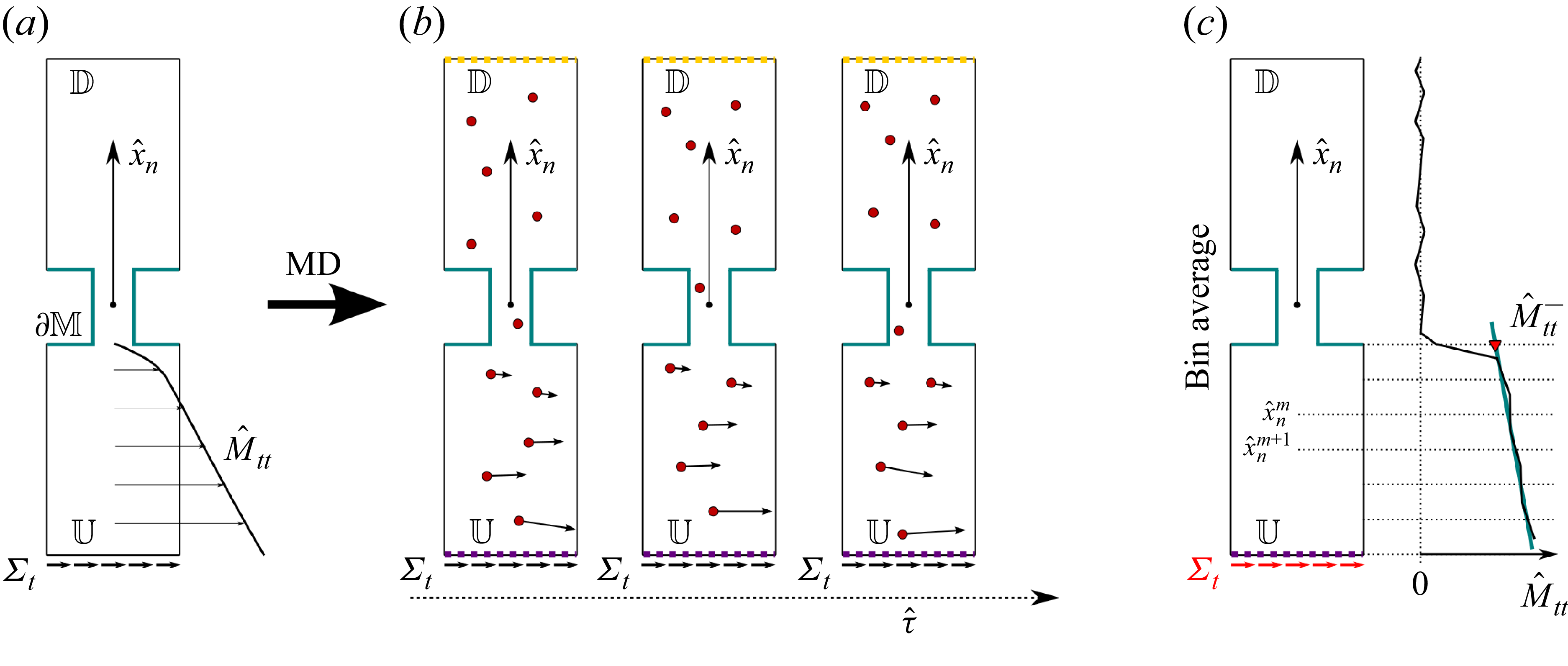
 Mtt±
 Mss±
 a
 b
 U
 Σt
 Σs
 t
 s
 U
 xtU
 xsU
 τ^
 U
 M^tt
 M^ss
 M^tt
 M^ss
 M^tt−
 M^ss−
 Mtt−
 Mss−

 a
 H2O
 U
 D
 C∗
 C
 ∂F
 x^t
 x^s
 b
 ∂F
 ℓt×ℓs
 ℓ=0.5(ℓt+ℓs)
 H
 a
 x^t
 x^s

 a
 Σn
 U
 F
 b−d
 U
 Σn=290,1990,6990 bar
 e
 a=4.8
 A˚
 a=4.8
 A˚
 a=2.4
 A˚
 f
 M^nn±
 U
 a=4.8
 A˚
 a=2.4
 A˚
 0.1
 ∂M
 a=4.8
 A˚
 a=2.4
 A˚
 ∂M
 a=4.8
 A˚
 a=2.4
 A˚
 g
 Mnn±
 f
 Mnn±

 a
 Σt
 U
 F
 M^tt
 (b−d)
 M^tt
 Σt=5,50,100 bar
 ∂M
 x^t=x^s=0
 ∂M
 U
 e
 M^tt
 Mtt=μM^tt/ℓΣt
 E
 M¯tt
 Σt>6 bar
 f
 e
 Mss−

 a
 C
 b
 4×4
 c
 A
 B
 x^1
 x^3
 ΣN
 A
 10bar
 B
 k×k
 k=40
 A˚
 h=100
 A˚
 d
 C
 C

 u^2
 A
 ∂M
 10bar
 B
 ΣN

 a
 C
 b
 C∗
 x^t
 Σt=5bar
 τ^=0
 400 ps

 Mnn
 a
 H
 ℓs=ℓt

 a
 a=58
 A˚
 ℓt=152
 A˚
 ℓs=153
 A˚
 H=51
 A˚
 b
 M^nn−
 ∂M
 ∂M

 Open access

