1 Introduction
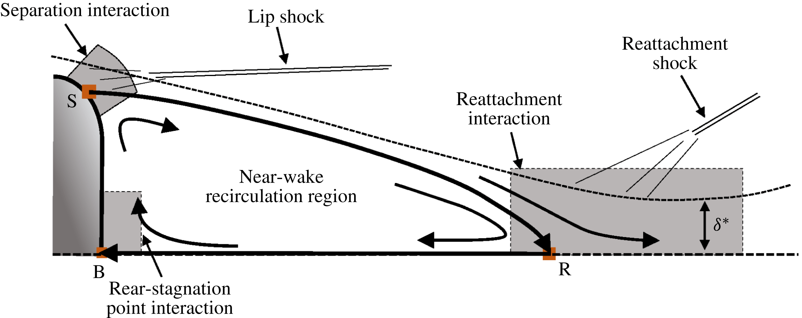
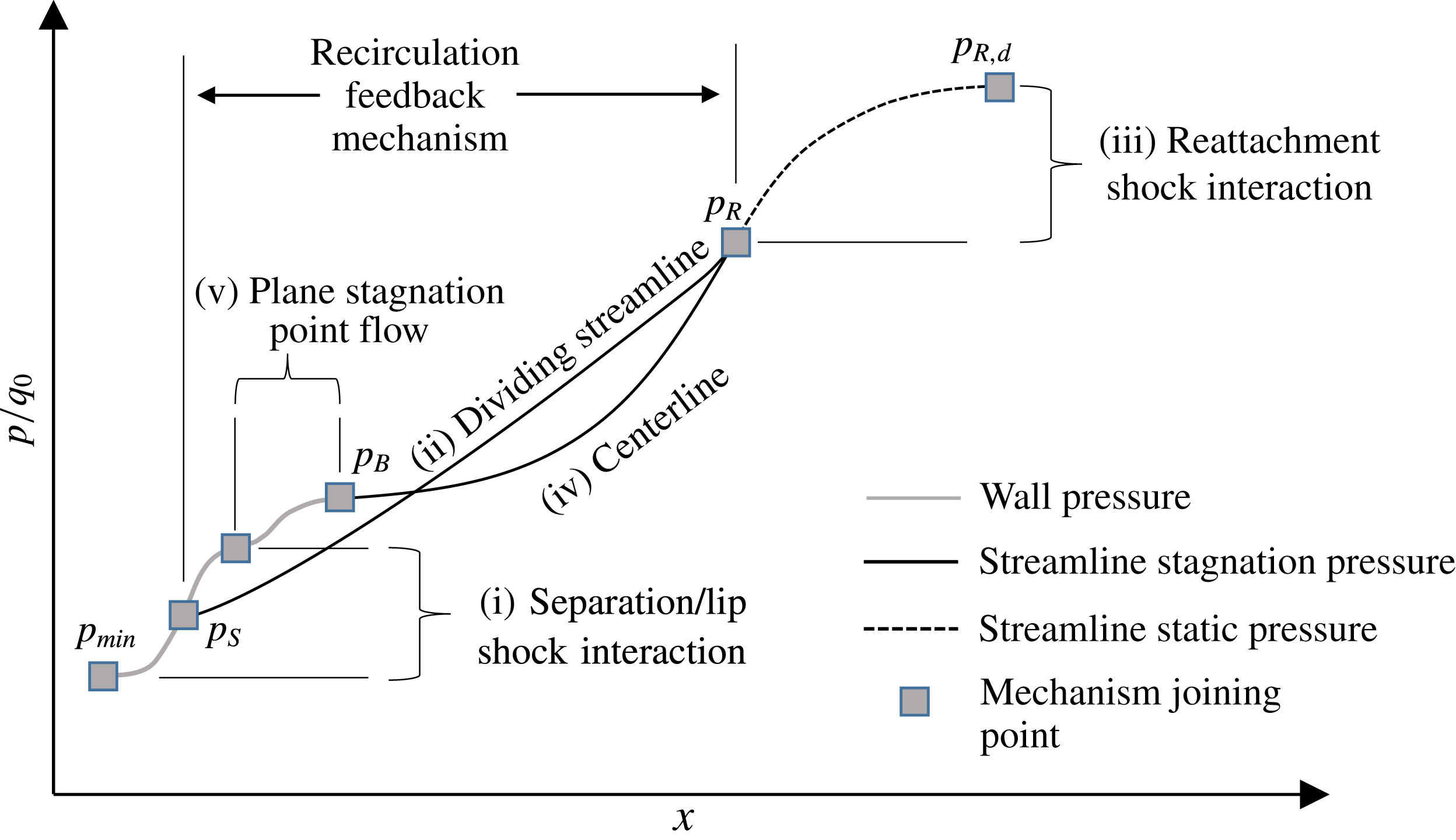
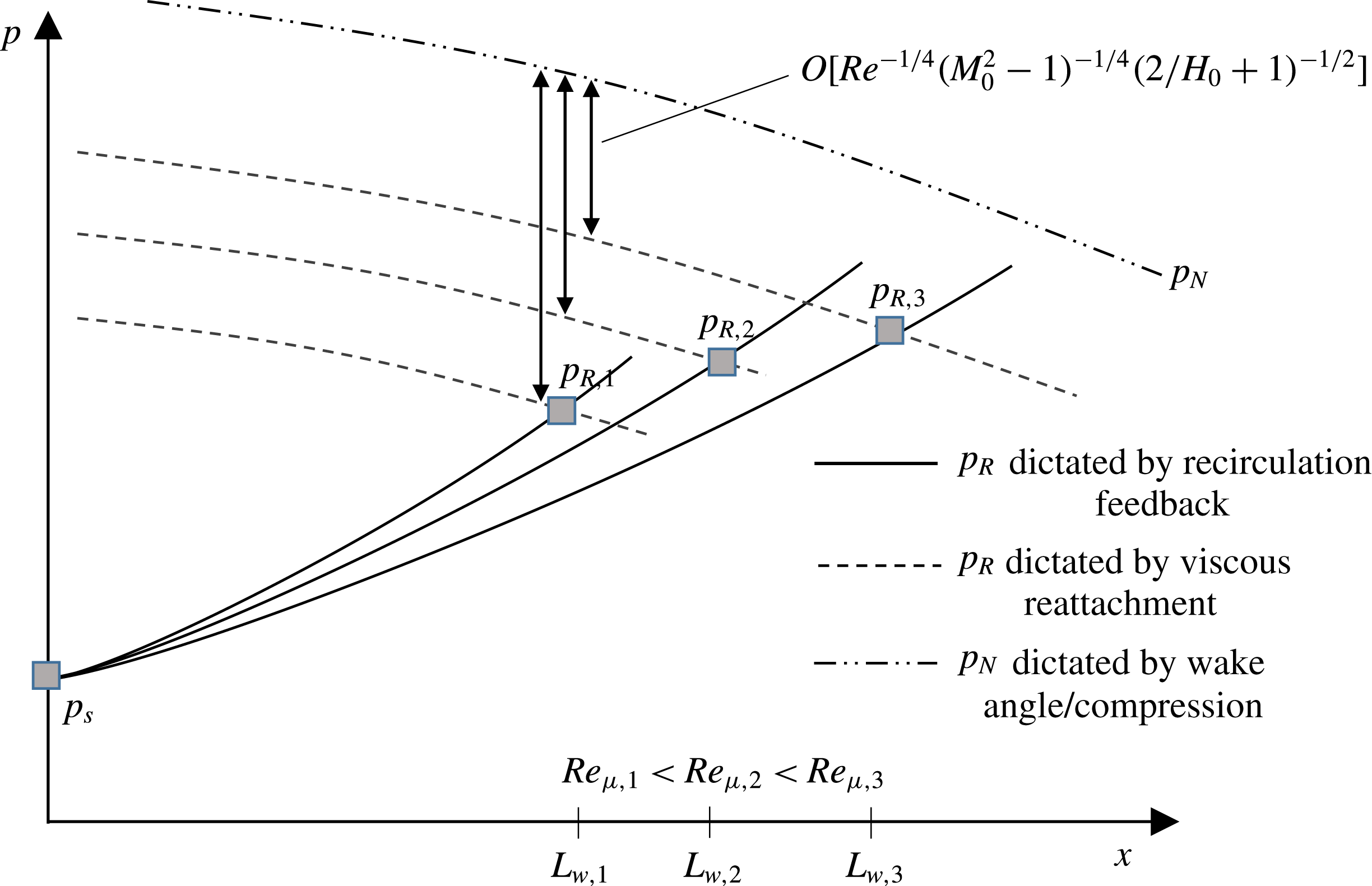
The hypersonic wake behind a blunt body is an important flow problem for the study of fluid mechanics and is practical for engineering applications such as atmospheric entry vehicles, satellites, meteors, bullets and ballistic missiles. Prominent features of the hypersonic near wake to be discussed in this paper are outlined in figure 1. The hypersonic wake or base-flow problem has been studied since the 1950s. The primary motivation for this field of study has been the contribution of the near wake to the drag of missile-type projectiles (as much as 30 %) (Delery & Lacau Reference Delery and Lacau1988). Prior to the advent of powerful modern computers to this field of research, extensive effort was given to predicting these flows through low-order analyses (Chapman Reference Chapman1950; Chapman, Kuehn & Larson Reference Chapman, Kuehn and Larson1958; Baum, King & Denison Reference Baum, King and Denison1964; Lees Reference Lees1964; Lees & Reeves Reference Lees and Reeves1964; Reeves & Lees Reference Reeves and Lees1965; Weinbaum Reference Weinbaum1966; Weiss Reference Weiss1966; Weiss & Weinbaum Reference Weiss and Weinbaum1966; Baum Reference Baum1967; Grange, Klineberg & Lees Reference Grange, Klineberg and Lees1967; Weiss Reference Weiss1967; Baum Reference Baum1968). Comprehensive reviews of these early analysis techniques can be found in Smith & Lamb (Reference Smith and Lamb1974) and Delery & Lacau (Reference Delery and Lacau1988). Experimental techniques typically included wall pressure measurements, Schlieren and shadowgraph visualizations and hot-wire anemometry (Chapman et al. Reference Chapman, Kuehn and Larson1958; Tewfik & Giedt Reference Tewfik and Giedt1960; McCarthy & Kubota Reference McCarthy and Kubota1964; Dewey Reference Dewey1965). The observations made in these works led to improved physical understanding and mathematical formulation of the near-wake/base-flow phenomena and allowed for the assessment of simple models. However, a persistent challenge in the investigation of the physics in supersonic base flows was the lack of off-body experimental data. Until the 1990s, high fidelity simulations of the Navier–Stokes equations and quantitative off-body measurements were not available. According to Dutton et al. (Reference Dutton, Herrin, Molezzi, Mathur and Smith1995), as of 1990 no off-body velocimetry for the supersonic base-flow problem was available. Recently, given the robustness of modern numerical techniques, state-of-the-art computer power, and the development of advanced laser diagnostics, work on the base-flow problem has received renewed attention.
Schematic of prominent near-wake flow features and interaction regions.

The vast majority of renewed interest in studying the fundamental fluid mechanics of the near wake has focused on the turbulent near wake of the flat base behind a cone or axially aligned cylinder or tube. For example, non-intrusive diagnostics have been performed on the compressible near wake of slender-cone and missile-type geometries using laser Doppler velocimetry (LDV) (Herrin & Dutton Reference Herrin and Dutton1994, Reference Herrin and Dutton1995), planar laser-induced fluorescence (PLIF) (Lachney & Clemens Reference Lachney and Clemens1998; Scarano & Van Oudheusden Reference Scarano and Van Oudheusden2003), particle image velocimetry (PIV) (Humble, Scarano & van Oudheusden Reference Humble, Scarano and van Oudheusden2007) and Mie scattering (Kastengren & Dutton Reference Kastengren and Dutton2005). As well, simulations of slender-cone and missile-type geometries have been performed using Reynolds-averaged Navier–Stokes (RANS), large-eddy simulation (LES) and detached-eddy simulation (DES) (Fureby, Nilsson & Andersson Reference Fureby, Nilsson and Andersson1999; Forsythe et al. Reference Forsythe, Hoffmann, Cummings and Squires2002; Kawai & Fujii Reference Kawai and Fujii2005; Simon et al. Reference Simon, Deck, Guillen and Sagaut2006, Reference Simon, Deck, Merlen, Guillen and Sagaut2007; Deck & Thorigny Reference Deck and Thorigny2007; Barnhardt & Candler Reference Barnhardt and Candler2012) to study the turbulent base-flow problem.
Several important differences exist between the hypersonic flow over slender-cone-type geometries and that of a blunt projectile such as a re-entry capsule. Firstly, the hypersonic near wake of blunt bodies maintains a laminar nature over a much wider range of Reynolds and Mach numbers than occur in a subsonic or low-supersonic blunt-body flow (Lees Reference Lees1964; McCarthy & Kubota Reference McCarthy and Kubota1964; Schneider Reference Schneider2008). This is due to several flow field characteristics. The most important of these characteristics are the decreased effective Reynolds number due to the bow shock, and the favourable pressure gradient that occurs because of the blunt body’s curvature. These effects preserve the laminar nature of the boundary layer and near wake to a much higher free-stream Reynolds number. Additionally, the application of these studies is primarily to vehicles that fly at high altitudes or in low density atmospheres and have a small characteristic length scale (such as micro-orbiters and sample return vehicles). For this reason, re-entry vehicles are often analysed assuming a laminar flow over the body and in the near wake (Mitcheltree & Gnoffo Reference Mitcheltree and Gnoffo1995; Wood, Gnoffo & Rault Reference Wood, Gnoffo and Rault1996; Olynick, Chen & Tauber Reference Olynick, Chen and Tauber1999; Ottens Reference Ottens2002; Walpot Reference Walpot2002; Otsu et al. Reference Otsu, Abe, Ohnishi, Sasoh and Takayama2002; Liever et al. Reference Liever, Habchi, Burnell and Lingard2003; Mehta Reference Mehta2006, Reference Mehta2008; Sinha & Dey Reference Sinha and Dey2010; McDaniel, Wright & Songer Reference McDaniel, Wright and Songer2011; Shang & Surzhikov Reference Shang and Surzhikov2011; Johnston & Brandis Reference Johnston and Brandis2015). The latest Mars Science Laboratory (MSL) capsule was one of the first Martian entry vehicles that was expected to experience turbulence at its peak heating flight condition (Hollis & Collier Reference Hollis and Collier2008). The rapid flow expansion around the vehicle’s shoulders has been observed to cause relaminarization of the boundary layer (Hollis et al. Reference Hollis, Berger, Horvath, Coblish, Norris, Lillard and Kirk2009). Due to the complex nature of the hypersonic near wake, extensive study is required to better understand dependencies and mechanisms that affect separation, lip-shock formation, base heating, momentum and energy transfer and wake topology.
The present state of understanding of the hypersonic blunt-body near wake is a matter of debate. This is largely due to the fact that the wake topology is very well observed and its understanding is not critical to estimate fore-body drag or heating. As well, in many cases the dependence of near-wake features on parameters such as Mach and Reynolds number are well observed and correlated empirically (such as separation location (Park, Gai & Neely Reference Park, Gai and Neely2010b ; Hinman & Johansen Reference Hinman and Johansen2016c ) and base pressure (Grasso & Pettinelli Reference Grasso and Pettinelli1995; Lamb & Oberkampf Reference Lamb and Oberkampf1995)). However, it is rare that these observations are explained using a complete physical mechanism. In many ways, the methods of analysis such as the Chapman (Reference Chapman1950) and the Crocco & Lees (Reference Crocco and Lees1952) theories, presented in the 1950s, still represent the state-of-the-art in terms of physical understanding. Despite its known limitations, Chapman theory is often used as a foundation to explain research results or even expanded upon to predict near-wake features (Grasso & Pettinelli Reference Grasso and Pettinelli1995; Park, Gai & Neely Reference Park, Gai and Neely2010a ; Park et al. Reference Park, Gai and Neely2010b ). As stated by Smith & Lamb (Reference Smith and Lamb1974), the fundamental assumptions in this model are known to be invalid yet the resulting empirical predictions are highly acceptable, explaining the continued use of these models.
Aside from work devoted to further understanding turbulence and transition in these scenarios, little work has been made to further investigate the underlying physical mechanisms driving observed trends in the laminar flow case. Until very recently, work utilizing modern experimental and numerical techniques were limited to project- and mission-based research. For example, new visualization techniques have been used to examine the hypersonic wakes of specific mission-based capsule geometries (Schrijer & Walpot Reference Schrijer and Walpot2010; Balla Reference Balla2013; Combs et al. Reference Combs, Clemens, Danehy, Bathel, Parker, Wadhams, Holden and Kirk2013; Johansen et al. Reference Johansen, Danehy, Ashcraft, Bathel, Inman and Jones2013a ). As well, simulations of vehicles have been performed using direct simulation Monte Carlo (DSMC) (Moss, Gupta & Price Reference Moss, Gupta and Price1996; Mitcheltree et al. Reference Mitcheltree, Wilmoth, Cheatwood, Brauckmann and Greene1997, Reference Mitcheltree, Moss, Cheatwood, Greene and Braun1999; Zhong, Ozawa & Levin Reference Zhong, Ozawa and Levin2008a ), laminar (Mitcheltree & Gnoffo Reference Mitcheltree and Gnoffo1995; Wood et al. Reference Wood, Gnoffo and Rault1996; Olynick et al. Reference Olynick, Chen and Tauber1999; Ottens Reference Ottens2002; Walpot Reference Walpot2002; Otsu et al. Reference Otsu, Abe, Ohnishi, Sasoh and Takayama2002; Liever et al. Reference Liever, Habchi, Burnell and Lingard2003; Mehta Reference Mehta2006, Reference Mehta2008; Sinha & Dey Reference Sinha and Dey2010; McDaniel et al. Reference McDaniel, Wright and Songer2011; Shang & Surzhikov Reference Shang and Surzhikov2011; Johnston & Brandis Reference Johnston and Brandis2015), RANS (Berger Reference Berger2009; Reddy & Sinha Reference Reddy and Sinha2009; Johansen et al. Reference Johansen, Novak, Bathel, Ashcraft and Danehy2013b ; Desikan et al. Reference Desikan, Patil and Subramanian2015), DES (Brock, Subbareddy & Candler Reference Brock, Subbareddy and Candler2015; Schwing & Candler Reference Schwing and Candler2015) and LES (Salazar & Edwards Reference Salazar and Edwards2014) models on many different project- and mission-based geometries.
The drawback of these types of studies is the limited general applicability of their results and conclusions. Due to the absence of a complete theoretical explanation of the near wake, contradictory or incomplete results are either not explained or ignored. For example, for the location of flow separation, many studies focus on combined Reynolds number and Mach number effects (Grasso & Pettinelli Reference Grasso and Pettinelli1995; Park et al. Reference Park, Gai and Neely2010b ; Hinman & Johansen Reference Hinman and Johansen2016c ) while others focus on Mach number, making no reference to Reynolds number (Liever et al. Reference Liever, Habchi, Burnell and Lingard2003; Mehta Reference Mehta2006, Reference Mehta2008; Nakamura, Manabe & Nishio Reference Nakamura, Manabe and Nishio2006) or observe insignificant effects of Reynolds number (Suzuki & Abe Reference Suzuki and Abe1994; Schrijer & Walpot Reference Schrijer and Walpot2010; Walpot et al. Reference Walpot, Wright, Noeding and Schrijer2012). Additionally, in some works both Mach and Reynolds number have been found to have little effect on observations in the wake (Zhong et al. Reference Zhong, Ozawa and Levin2008a ). Clearly, it is not an inability to predict or simulate hypersonic wake flows that is the present limitation in this field of study; it is an inability to understand, discuss and compare.
Recent experimental and numerical works have tried to fill the gap in this area of research by focusing on more basic (and therefore more general) geometries. For example, empirical relationships for separation location on a circular cylinder as a function of Reynolds number have been presented by Park et al. (Reference Park, Gai and Neely2010b ) and more recently by Hinman & Johansen (Reference Hinman and Johansen2016c ). New experimental imaging has recently been done by Hruschka, O’Byrne & Kleine (Reference Hruschka, O’Byrne and Kleine2008, Reference Hruschka, O’Byrne and Kleine2010, Reference Hruschka, O’Byrne and Kleine2011) and Schmidt & Shepherd (Reference Schmidt and Shepherd2015) on more generic shapes. The most recent experiment by Hruschka et al. (Reference Hruschka, O’Byrne and Kleine2011) is believed to be the first non-intrusive, sting-free velocimetry of the hypersonic blunt-body near wake. Simulations have been performed by Grasso & Pettinelli (Reference Grasso and Pettinelli1995), Bashkin et al. (Reference Bashkin, Egorov, Egorova and Ivanov1998, Reference Bashkin, Vaganov, Egorov, Ivanov and Ignatova2002), Park, Gai & Neely (Reference Park, Gai and Neely2016) and Hinman & Johansen (Reference Hinman and Johansen2016a ,Reference Hinman and Johansen c ). The recent ramping up of generic blunt-body hypersonic wake research has led to a greater understanding of the topology and physical mechanisms at work. This study aims to continue this trend by focusing on the dominant mechanisms that have been observed in the hypersonic laminar near wake.
The hypersonic blunt-body flow problem is highly complex. Chemical reactions, chemical and thermal non-equilibrium, rarefied flow, turbulence, ablation, three dimensionality and unsteadiness are all relevant within certain ranges of flight conditions. These effects are known to modify the flow field and are important. However, many of these effects may be best understood or explained as modifications of the underlying mechanisms of the most basic flow field. Therefore, this work is focused on the fundamental underlying aspects through the study of two-dimensional/axisymmetric, adiabatic laminar continuum flow that is in thermal and chemical equilibrium over a simple blunt-body geometry. The objectives of the present work are:
-
(i) to develop a near-wake mechanism that can be used to explain observed near-wake dependencies;
-
(ii) to develop a semi-empirical relationship between the free-stream properties (
 $Re_{\infty }$
,
$M_{\infty }$
) and the wake Reynolds number,
$Re_{w,h}$
;
-
(iii) to use the new developed overall near-wake mechanism and wake Reynolds number relation to explain experimental and numerical results found in the literature;
-
(iv) to use the presented wake mechanism to discuss the potential impact of a wake sting on near-wake flow.


To examine the theoretical work presented, new simulations have been performed and are supplemented by legacy datasets generated in previous work (Hinman & Johansen Reference Hinman and Johansen2016c ). A new grid independence study has been performed on two planar simulations where higher-order parameters in the wake are extracted for analysis. Additionally, new axisymmetric simulations of an adiabatic sphere have been performed. A detailed explanation of simulation set-up can be found in § 2. In §§ 3 to 4, multiple analyses are carried out using the simulation data as material for comparison and discussion. In § 5, the present theoretical framework for the hypersonic laminar near wake is summarized. This framework is then used to perform a disambiguation of observations from simulations and experiments found in the literature.
2 Simulation details
Computational fluid dynamics (CFD) simulations were completed for flow over an adiabatic circular cylinder at Reynolds numbers of
 $10^{4}$
,
 $10^{5}$
and Mach 6. As well, simulations (sparsely distributed) over a range of Mach 6–10 and
 $Re_{\infty ,L}=10^{4}$
–
 $10^{5}$
have been performed for an adiabatic sphere. All simulations were performed using the open-source CFD software, OpenFOAM. Specifically, the compressible Navier–Stokes equations solver rhoCentralFOAM was used:
 $$\begin{eqnarray}\displaystyle & \displaystyle \frac{\unicode[STIX]{x2202}\unicode[STIX]{x1D70C}}{\unicode[STIX]{x2202}t}+\unicode[STIX]{x1D735}\boldsymbol{\cdot }(\unicode[STIX]{x1D70C}\boldsymbol{V})=0, & \displaystyle\end{eqnarray}$$
 $$\begin{eqnarray}\displaystyle & \displaystyle \frac{\unicode[STIX]{x2202}(\unicode[STIX]{x1D70C}\boldsymbol{V})}{\unicode[STIX]{x2202}t}+\unicode[STIX]{x1D735}\boldsymbol{\cdot }\left[\boldsymbol{V}\left(\unicode[STIX]{x1D70C}\boldsymbol{V}\right)\right]+\unicode[STIX]{x1D735}p-\unicode[STIX]{x1D735}\boldsymbol{\cdot }\unicode[STIX]{x1D70F}=0, & \displaystyle\end{eqnarray}$$
 $$\begin{eqnarray}\displaystyle & \displaystyle \frac{\unicode[STIX]{x2202}\unicode[STIX]{x1D70C}E}{\unicode[STIX]{x2202}t}+\unicode[STIX]{x1D735}\boldsymbol{\cdot }(\boldsymbol{V}(\unicode[STIX]{x1D70C}E))+\unicode[STIX]{x1D735}\boldsymbol{\cdot }[\boldsymbol{V}p]-\unicode[STIX]{x1D735}\boldsymbol{\cdot }(\unicode[STIX]{x1D70F}\boldsymbol{\cdot }\boldsymbol{V})+\unicode[STIX]{x1D735}\boldsymbol{\cdot }j=0, & \displaystyle\end{eqnarray}$$
where
 $\unicode[STIX]{x1D70C}$
,
 $V$
,
 $p$
,
 $E$
,
 $\unicode[STIX]{x1D70F}$
and
 $j$
are density, velocity, pressure, total energy, the shear stress tensor and diffusive heat flux tensor, respectively.
The temperature-dependent gas properties were modelled using known empirical relations. Nitrogen (
 $\text{N}_{2}$
) was used as the simulated test gas. The molecular viscosity was modelled using Sutherland’s law. The specific heat capacity and specific enthalpy were modelled using a 7-coefficient NASA polynomial based on the NIST-JANAF database (NIST-JANAF 2013). The thermal conductivity was modelled using the aforementioned models and the modified Eucken formula (Poling, Prausnitz & O’Connell Reference Poling, Prausnitz and O’Connell2001). The solver rhoCentral-FOAM as well as the thermophysical models have been used together by the present authors to study similar hypersonic flow problems (Arisman & Johansen Reference Arisman and Johansen2015; Arisman et al.
Reference Arisman, Johansen, Bathel and Danehy2015; Hinman & Johansen Reference Hinman and Johansen2016a
,Reference Hinman and Johansen
b
,Reference Hinman and Johansen
c
) and found good agreement to alternative models, solvers and experimental data.
2.1 Computational grid
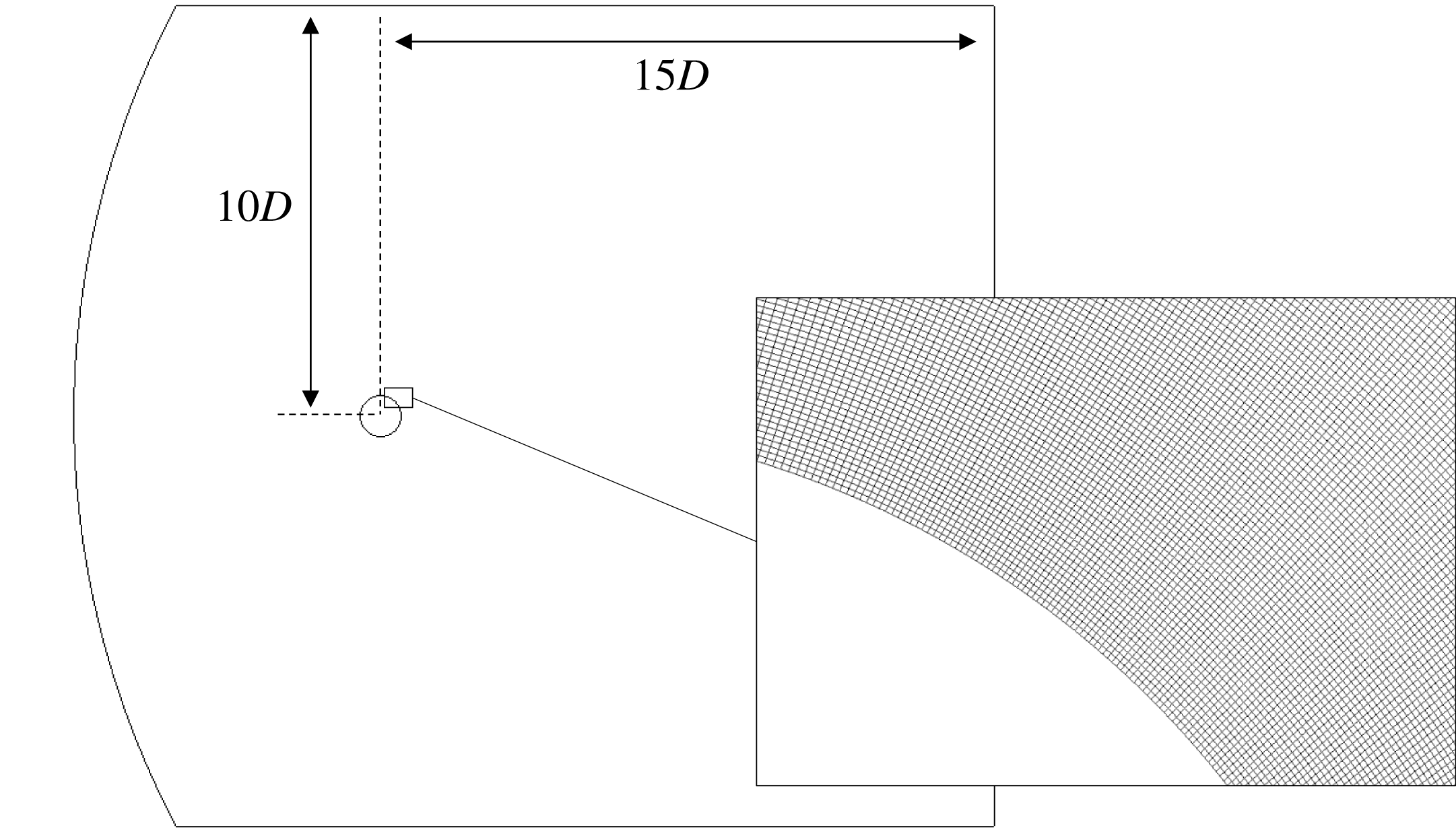
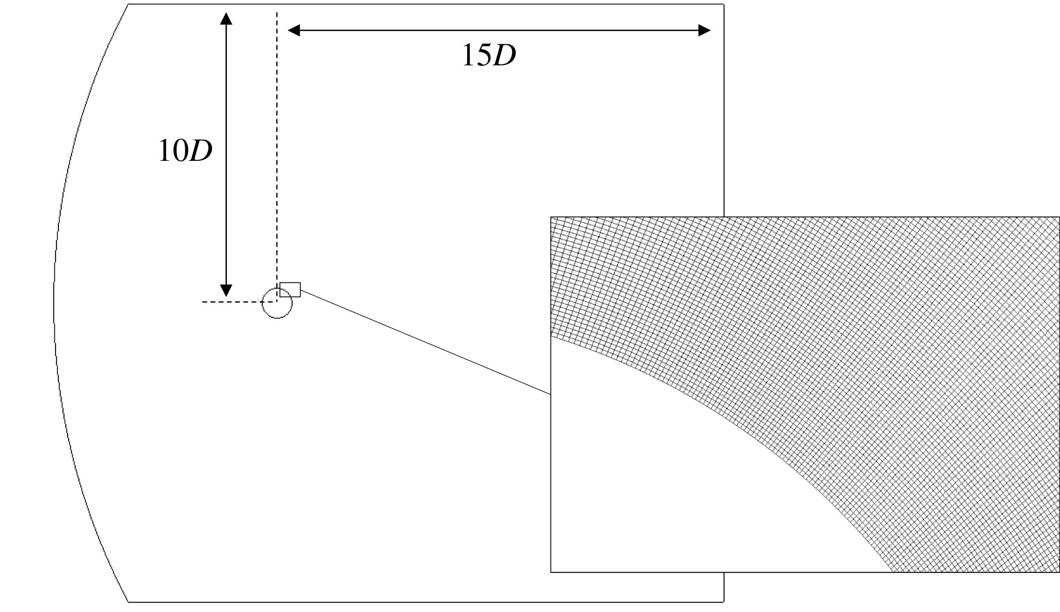
In the present work, off-body variables and derivatives are of interest. For this reason, a new computational grid was created with improved topology from previous studies and a new grid independence study has been performed on the wake parameters of interest. The computational grid was created using the commercial software Pointwise using a structured blocking technique. The grid produced by Pointwise was then converted to an unstructured grid, which is required by OpenFOAM. Previous experience with developing grids for OpenFOAM has found that the presence of high aspect ratio cells in the region of the viscous separation interaction leads to inconsistent results. In this region strong gradients are produced in both principal directions and therefore cells of relatively low aspect ratio (
 ${<}2$
) are preferred. A picture of the computational domain and the cells in this region is shown in figure 2.
Computational domain and grid in separation region (showing
 $0.25\times$
fine grid density).
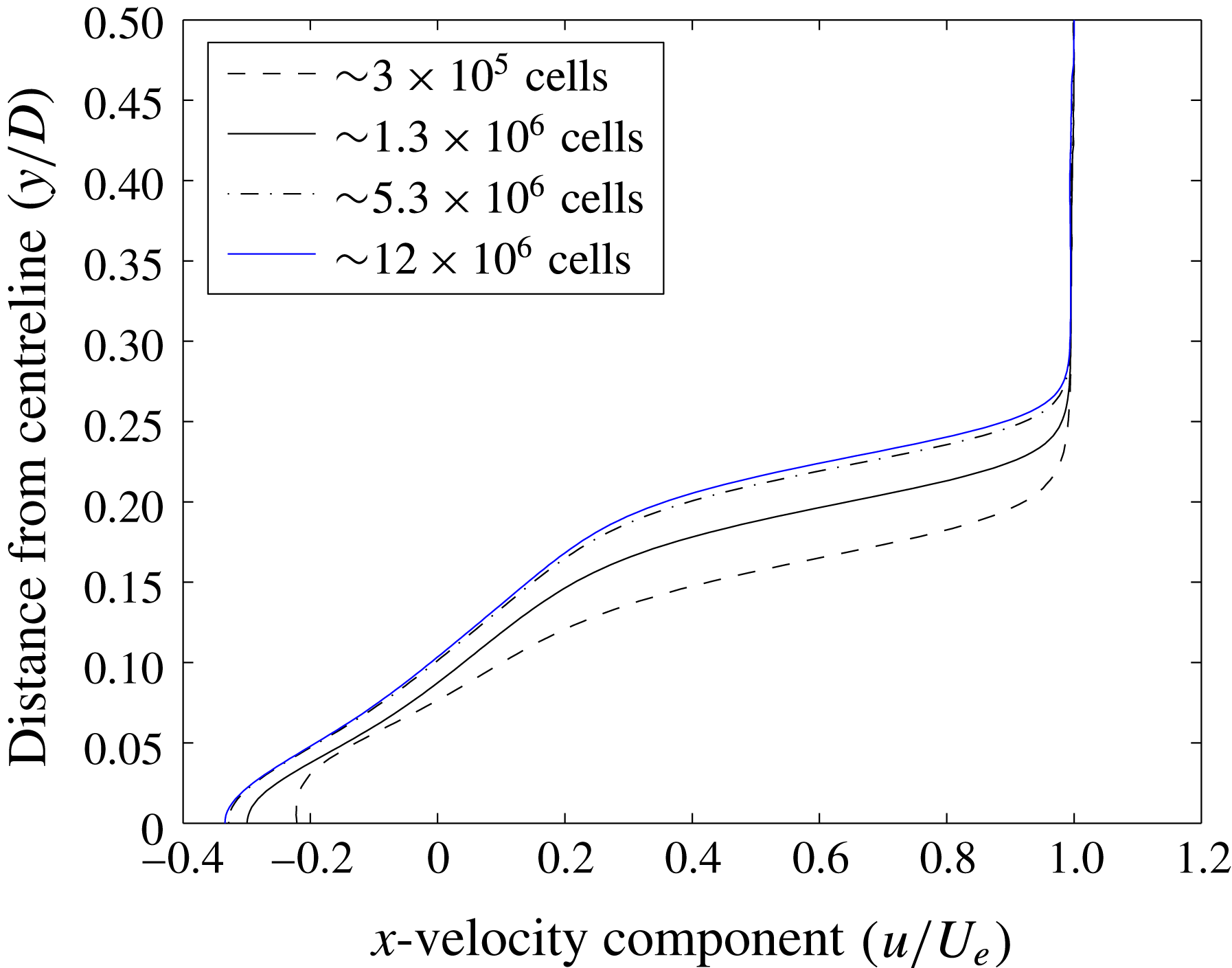
Velocity (
 $x$
-component –
 $\boldsymbol{V}\boldsymbol{\cdot }\hat{i} \,$
) profile at
 $x=0.5D$
from base.
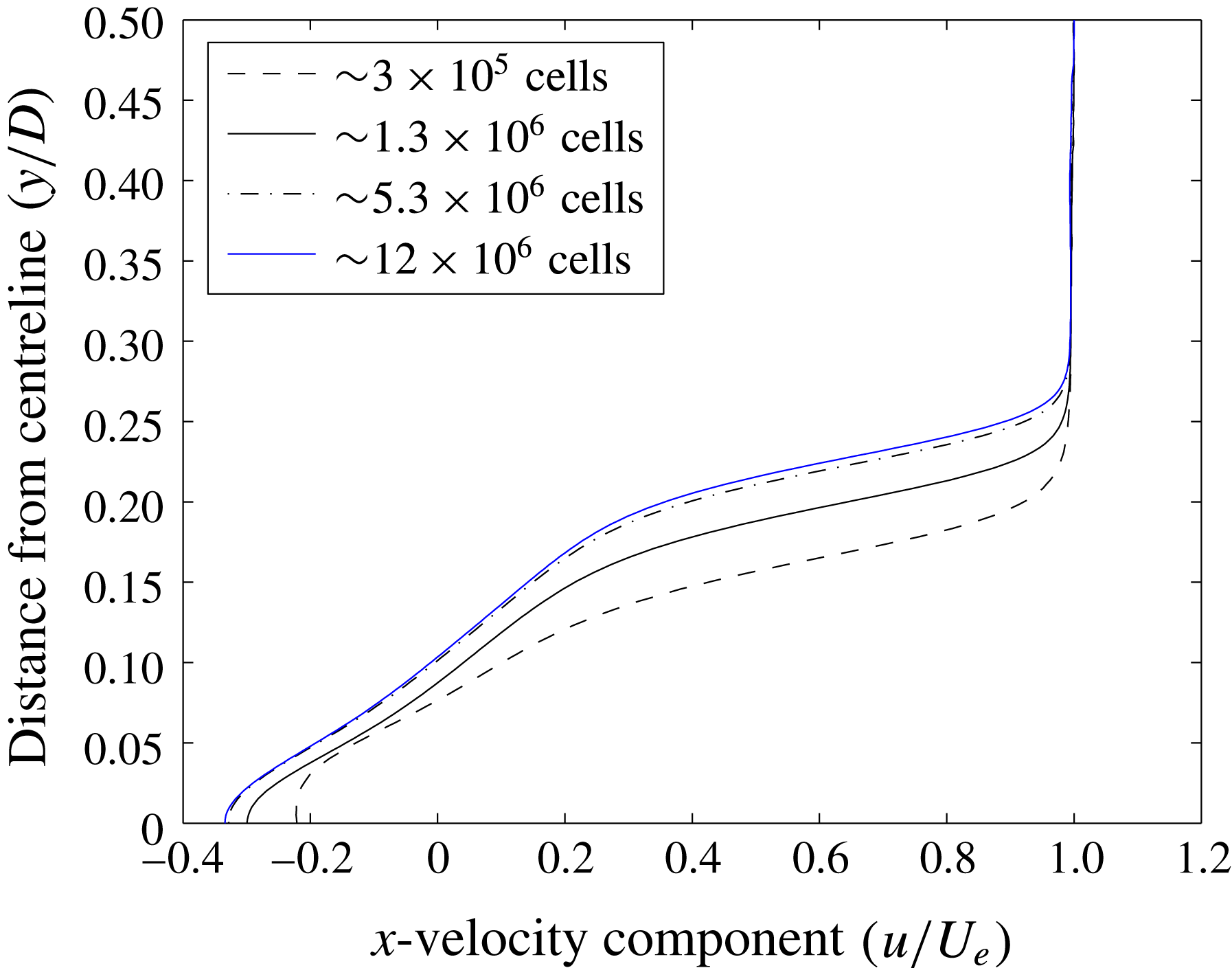
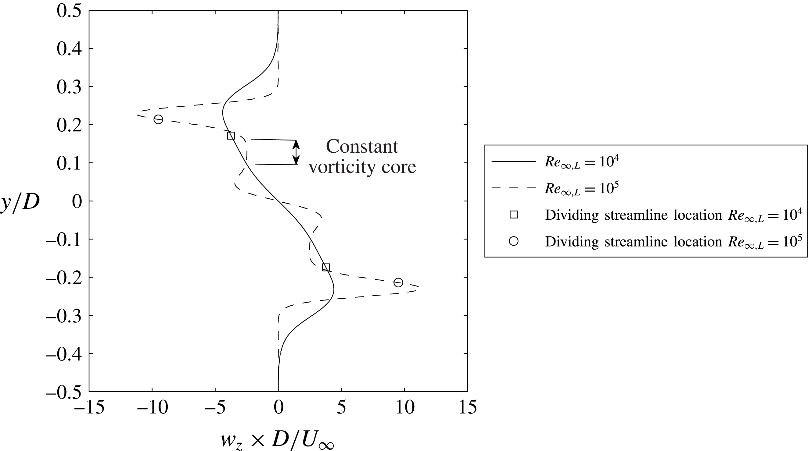
To establish grid independence, velocity profiles in the wake were examined at four grids of increasing grid density. The most demanding case in terms of grid requirements corresponds to the highest Reynolds number case (
 $Re_{\infty ,L}=10^{5}$
). The effect of spatial resolution on vertical distributions of the
 $x$
-component velocity at
 $x/D=0.5$
is shown in figure 3. The maximum difference for centreline reversed flow velocity between the finest and second finest grids is less than 2 %. A similar grid dependence was observed for the other primitive flow variables in the wake (
 $p$
,
 $T$
,
 $V_{y}$
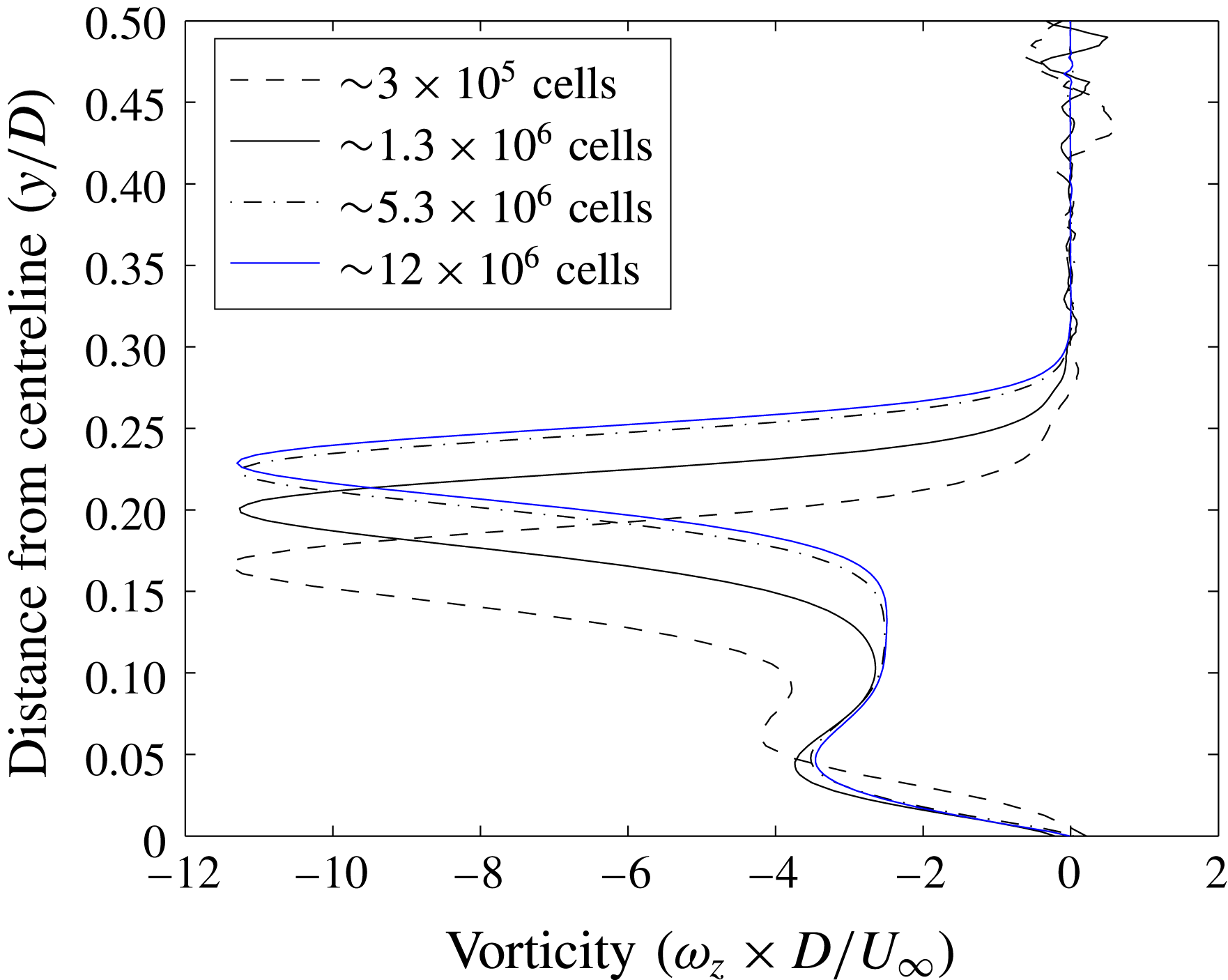
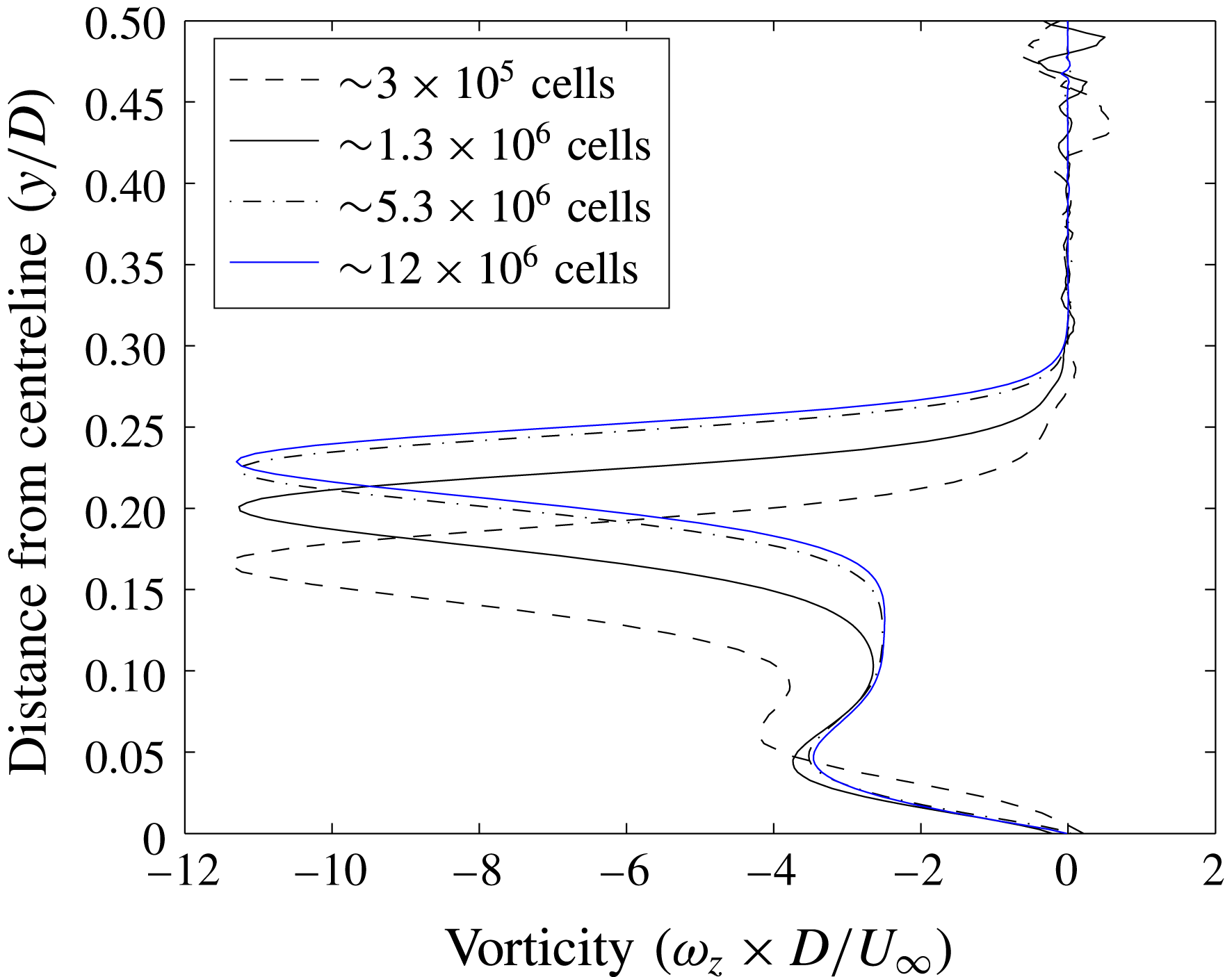
). Vorticity, a first derivative, was examined along the same line at
 $x/D=0.5$
(figure 4). The low Reynolds number case (
 $Re=10^{4}$
) was not simulated on the finest grid. Because of the decreased requirements for grid refinement at this Reynolds number it was found that 5.3 million cells was sufficient. Wall properties were also examined for the low and high Reynolds number case. At the wall, an average grid convergence index (GCI) of
 ${<}3\,\%$
was found for pressure, wall shear stress and adiabatic wall temperature. A similar set-up and convergence study was used for the simulations of flow over an adiabatic sphere.
Vorticity (
 $\unicode[STIX]{x1D714}_{z}$
) profile at
 $x=0.5D$
from base.
2.2 Legacy data
To supplement simulation data produced in the current work, data from previous work (Hinman & Johansen Reference Hinman and Johansen2016a
,Reference Hinman and Johansen
c
) by the authors were also used. Previously, simulations of hypersonic flow over adiabatic circular cylinders were performed for a range of Mach (
 $6<M_{\infty }<10$
) and Reynolds numbers (
 $8\times 10^{3}<Re_{\infty ,L}<8\times 10^{4}$
). In these previous works, the focus was on separation location, wall shear stress and pressure. A detailed grid convergence study was performed for these parameters (Hinman & Johansen Reference Hinman and Johansen2016c
). These data were used to facilitate analysis of a modified free-interaction theory at separation.
3 Analysis of wake character
In this section, the character of the near-wake recirculation region is analysed through a discussion of local Reynolds number, observations of the recirculation region topology and the link between these and the free-stream Mach and Reynolds number.
3.1 Wake Reynolds number analysis
According to Grasso & Pettinelli (Reference Grasso and Pettinelli1995) free-stream Mach and Reynolds numbers (based on a traditional characteristic length) are not useful in describing the wake topology because they do not account the flow features that occur upstream from the wake. Therefore, a wake Reynolds number should be used. Following the work of Weiss (Reference Weiss1966) and Grasso & Pettinelli (Reference Grasso and Pettinelli1995), a semi-empirical relationship between the wake and free-stream Reynolds number is derived here for laminar flow over an adiabatic blunt body. From Weiss (Reference Weiss1966) and Grasso & Pettinelli (Reference Grasso and Pettinelli1995), the characteristic wake Reynolds number should be based on the properties in the recirculation region or along the dividing streamline. For the appropriate wake length scale, the base half-height is used. Thus the preferred wake Reynolds number
 $Re_{w,h}$
is given by:
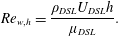 $$\begin{eqnarray}\displaystyle & \displaystyle Re_{w,h}=\frac{\unicode[STIX]{x1D70C}_{DSL}U_{DSL}h}{\unicode[STIX]{x1D707}_{DSL}}. & \displaystyle\end{eqnarray}$$
The temperature along the dividing streamline (
 $T_{DSL}$
) is calculated assuming a constant energy through the shear layer (and a recovery factor of
 $\sqrt{Pr}$
). Assuming a
 $2/3$
power law for the temperature dependence of viscosity, the relationship between free-stream Reynolds number to wake Reynolds number is:
 $$\begin{eqnarray}\displaystyle & \displaystyle Re_{w,h}=\frac{\unicode[STIX]{x1D70C}_{DSL}U_{DSL}h}{\unicode[STIX]{x1D707}_{DSL}}=\left(\frac{U_{DSL}}{U_{\infty }}\right)\left(\frac{\unicode[STIX]{x1D70C}_{DSL}}{\unicode[STIX]{x1D70C}_{\infty }}\right)\left(\frac{T_{\infty }}{T_{DSL}}\right)^{2/3}\left(\frac{h}{L}\right)Re_{\infty ,L}. & \displaystyle\end{eqnarray}$$
The ratio
 $h/L$
is the ratio between the half-base height and the length scale used to calculate free-stream Reynolds number. In the present case,
 $L$
is equivalent to the cylinder diameter
 $D$
. Using the definition of Mach number and the ideal gas law, this becomes:
 $$\begin{eqnarray}\displaystyle & \displaystyle \frac{Re_{w,h}}{Re_{\infty ,L}}=\left(\frac{M_{DSL}}{M_{\infty }}\right)\left(\frac{p_{DSL}}{p_{\infty }}\right)\left(\frac{T_{DSL}}{T_{\infty }}\right)^{-7/6}\left(\frac{h}{L}\right). & \displaystyle\end{eqnarray}$$
Using known relationships for isentropic flow, normal shocks and adiabatic recovery temperature, the ratios found in (3.3) have been derived:
 $$\begin{eqnarray}\displaystyle \displaystyle \frac{M_{DSL}}{M_{\infty }} & = & \displaystyle \frac{u^{\ast }M_{e}}{M_{\infty }\left(1+\displaystyle \frac{\unicode[STIX]{x1D6FE}-1}{2}M_{e}^{2}\left(\sqrt{Pr}-u^{\ast 2}\right)\right)},\end{eqnarray}$$
 $$\begin{eqnarray}\displaystyle \frac{p_{DSL}}{p_{\infty }} & = & \displaystyle \left(\frac{p_{B}}{p_{o,2}}\right)\left(\frac{\left(\unicode[STIX]{x1D6FE}+1\right)M_{\infty }^{2}}{\left(\unicode[STIX]{x1D6FE}-1\right)M_{\infty }^{2}+2}\right)^{\unicode[STIX]{x1D6FE}/(\unicode[STIX]{x1D6FE}-1)}\left(\frac{\left(\unicode[STIX]{x1D6FE}+1\right)}{2\unicode[STIX]{x1D6FE}M_{\infty }^{2}-\left(\unicode[STIX]{x1D6FE}-1\right)}\right)^{1/(\unicode[STIX]{x1D6FE}-1)}\nonumber\\ \displaystyle & & \displaystyle \times \,\left(1+\frac{\unicode[STIX]{x1D6FE}-1}{2}M_{\infty }^{2}\right)^{\unicode[STIX]{x1D6FE}/(\unicode[STIX]{x1D6FE}-1)},\end{eqnarray}$$
 $$\begin{eqnarray}\displaystyle \displaystyle \frac{T_{DSL}}{T_{\infty }} & = & \displaystyle \frac{1+\displaystyle \frac{\unicode[STIX]{x1D6FE}-1}{2}\left(\sqrt{Pr}-u^{\ast 2}\right)M_{e}^{2}}{1+\displaystyle \frac{\unicode[STIX]{x1D6FE}-1}{2}M_{e}^{2}}\left(1+\displaystyle \frac{\unicode[STIX]{x1D6FE}-1}{2}M_{\infty }^{2}\right),\end{eqnarray}$$
 $$\begin{eqnarray}\displaystyle \displaystyle M_{e} & = & \displaystyle \left[\left(\left(\frac{p_{B}}{p_{o,2}}\right)^{1-\unicode[STIX]{x1D6FE}/(\unicode[STIX]{x1D6FE})}-1\right)\frac{2}{\unicode[STIX]{x1D6FE}-1}\right]^{0.5}.\end{eqnarray}$$
In (3.4) to (3.7) the ratios
 $h/L$
,
 $p_{B}/p_{o,2}$
and
 $u^{\ast }$
must be approximated empirically. The height of the wake, and therefore
 $h/L$
, depends on separation location and vehicle geometry. For the present comparison to circular cylinder, the empirical formula for separation location from Hinman & Johansen (Reference Hinman and Johansen2016c
) is used to approximate this ratio as a function of post-shock Reynolds number:

From the works of McCarthy & Kubota (Reference McCarthy and Kubota1964), Dewey (Reference Dewey1965), Park et al. (Reference Park, Gai and Neely2010b
) and Hinman & Johansen (Reference Hinman and Johansen2016c
), it is observed that the base pressure is typically close to
 $p_{B}/p_{o,2}=0.03\pm 0.01$
for a circular cylinder over a wide range of Mach and Reynolds number. The value of
 $u^{\ast }$
for the Chapman similarity profile is 0.587. However, (as pointed out by Denison & Baum (Reference Denison and Baum1963)) this value is typically not reached. For the present calculations, a value of 0.3 was used. For geometries other than a circular cylinder, different values should be chosen for these variables (
 $h/L$
,
 $p_{b}/p_{o,2}$
and
 $u^{\ast }$
) by empirical estimates or more rigorous mathematical modelling.
While the current work is primarily focused on an adiabatic wall for simplicity, it is useful to derive an expression for vehicles with an isothermal wall. For example, in § 5.3, vehicles with non-adiabatic wall temperatures are analysed. Therefore, a relationship for the wake Reynolds number for non-adiabatic cases is also derived here. To approximate this case, the dividing streamline temperature is approximated as the average between the isoenergetic temperature and the wall temperature. The basis of this approximation is the fact that the
 $DSL$
originates at the wall (at
 $T_{w}$
) and then must be heated to some fraction of the viscous recovery temperature. The following equation gives the approximation for
 $T_{DSL}/T_{\infty }$
in this case:
 $$\begin{eqnarray}\displaystyle & \displaystyle \frac{T_{DSL}}{T_{\infty }}=\frac{1}{2}\left[\displaystyle \frac{1+\displaystyle \frac{\unicode[STIX]{x1D6FE}-1}{2}\left(\sqrt{Pr}-u^{\ast 2}\right)M_{e}^{2}}{1+\displaystyle \frac{\unicode[STIX]{x1D6FE}-1}{2}M_{e}^{2}}\left(1+\displaystyle \frac{\unicode[STIX]{x1D6FE}-1}{2}M_{\infty }^{2}\right)+\frac{T_{w}}{T_{\infty }}\right]. & \displaystyle\end{eqnarray}$$
Next, actual wake Reynolds numbers calculated from simulation data are compared to the wake Reynolds number calculated from (3.3). To accomplish this, the properties along the dividing streamline in the simulation results are spatially averaged:
 $$\begin{eqnarray}\displaystyle & \displaystyle Re_{w,h,CFD}=\frac{\bar{\unicode[STIX]{x1D70C}}_{DSL}\bar{u}_{DSL}h}{\bar{\unicode[STIX]{x1D707}}_{DSL}}. & \displaystyle\end{eqnarray}$$
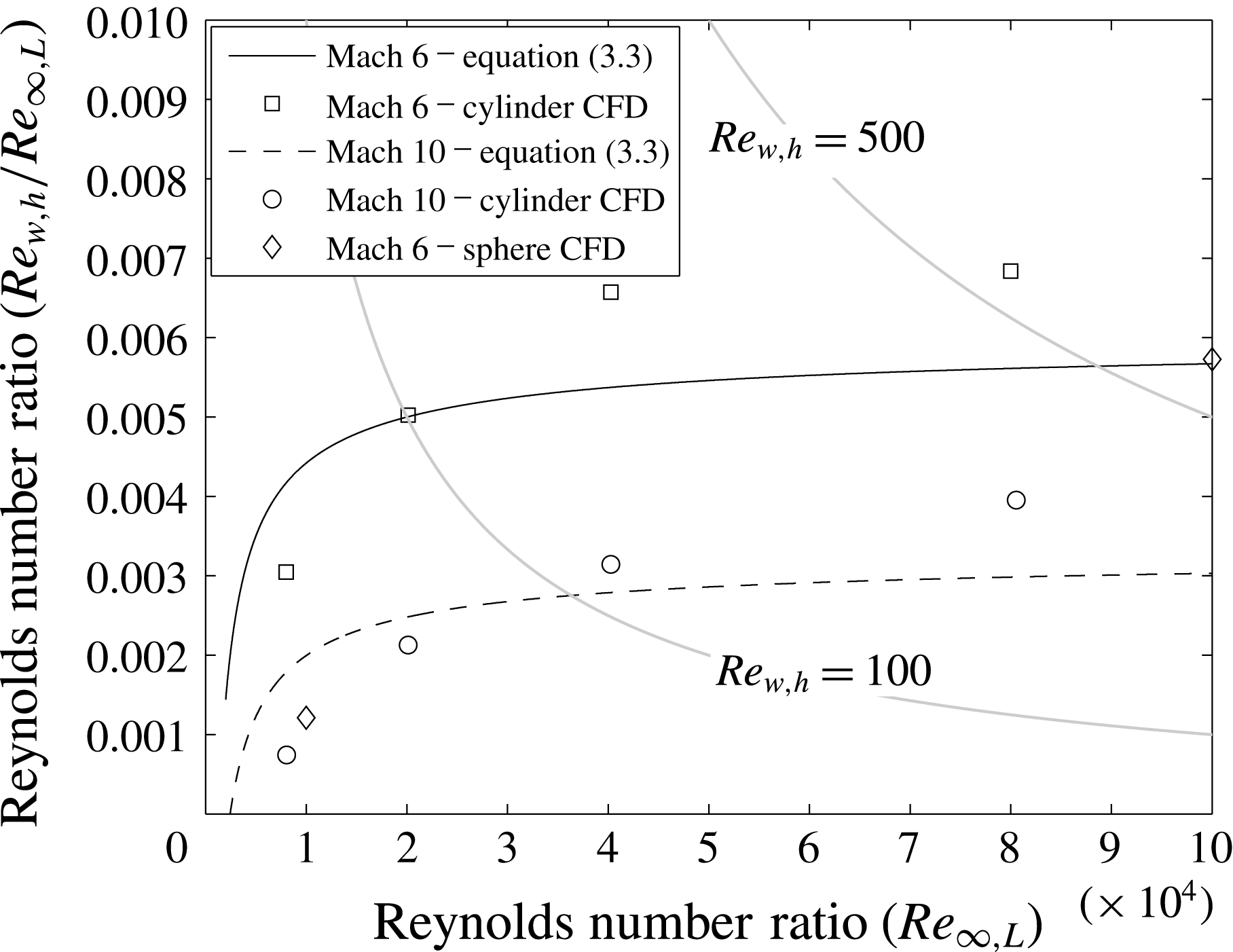
Equation (3.3) is plotted in figure 5. The simulation results for a range of Reynolds numbers at approximately Mach 6 and 10 are shown.
Comparison of equation (3.3) to CFD results for Reynolds number ratio.
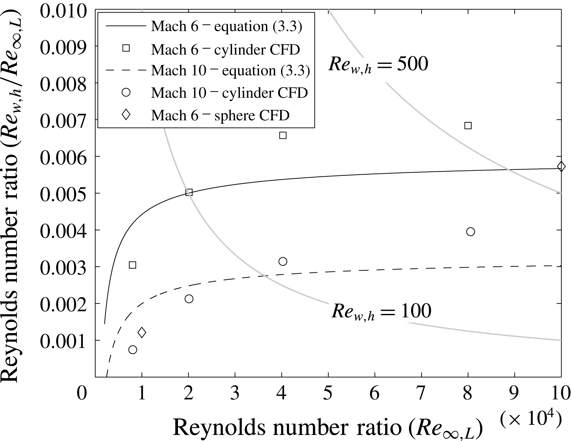
The results of (3.3) show qualitative agreement to the CFD data points with an appropriate order of magnitude. The difference between (3.3) and the CFD data is likely due to the empiricism in the equation formulation, as well as modelling in the CFD that is not accounted for. For example, in the simulations, the temperature-dependent gas properties vary through the shock and therefore the post-shock temperature is reduced. More substantial error is observed between (3.3) and CFD results for the adiabatic sphere at low Reynolds numbers. This is likely because the approximated variables (
 $p_{B}/p_{o,2}$
and
 $u^{\ast }$
) are different for the axisymmetric case and may possess increased Reynolds number dependence.
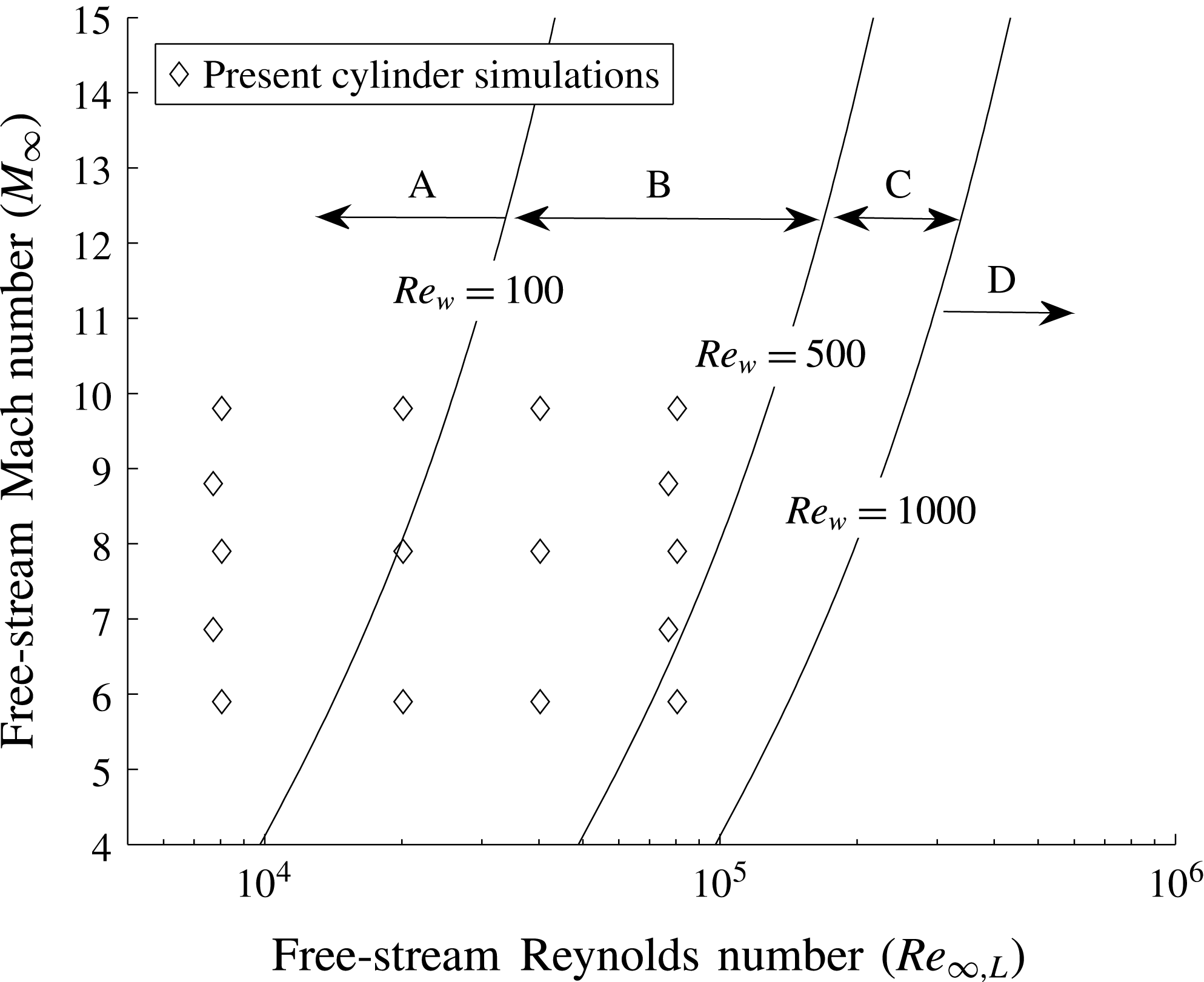
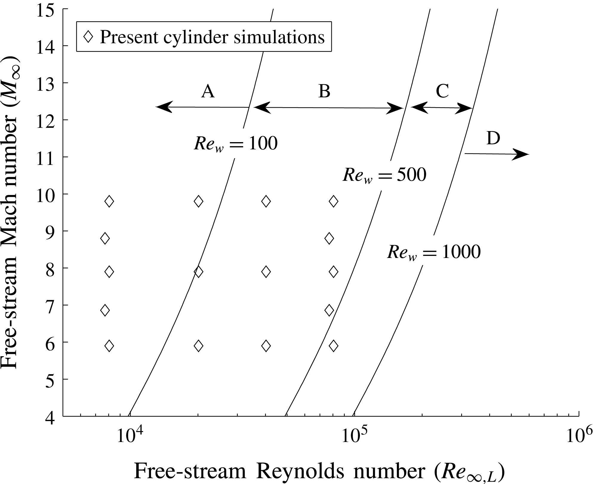
Equation (3.3) is a general approximation of the wake Reynolds number ratio. Therefore it can be used along with the criteria given by Grasso & Pettinelli (Reference Grasso and Pettinelli1995) to predict the nature of the wake. Lines of constant wake Reynolds number are plotted in figure 6 as a function of the free-stream Mach and Reynolds number. For reference, the coverage of the planar simulations from the present work are shown. The topological regimes (A–D) can be described as follows. Regime A is the regime of diffusion dominated wake flow. In this regime there is no central region of constant vorticity. In the work of Weiss (Reference Weiss1966) this regime was described as ‘Stokes-like’. In wake regime B, the flow is convective, but diffusion continues to dominate over advection. As Reynolds number increases, a region of constant vorticity appears and grows in size. Flow regime C is the regime where a secondary vortex appears in the corner of the wake flow. It is not clear whether the flow in this regime is safely considered to be laminar. In flow regime D, the flow is highly convective and both the primary and secondary wake vortex develop constant vorticity cores of increasing size. Regime D is where the transition to turbulence and unsteadiness in the near wake is expected to occur.
Relationship of free-stream Mach and Reynolds number to wake Reynolds number.
3.2 Observations of wake diffusion dominance
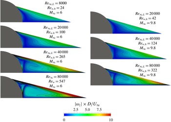
In the works of both Weiss (Reference Weiss1966) and Grasso & Pettinelli (Reference Grasso and Pettinelli1995) (following Batchelor (Reference Batchelor1956)) the vorticity profiles were an important point of discussion. In the previous sections it was shown that the characteristic wake Reynolds number is several orders of magnitude smaller than the corresponding free-stream value and a semi-empirical expression was derived. To examine this further, the variation of wake topology in the present simulations is examined and compared to the respective Reynolds number regimes from Grasso & Pettinelli (Reference Grasso and Pettinelli1995) and the expression derived in the previous section.
Vorticity contours at various wake Reynolds numbers (planar wake).
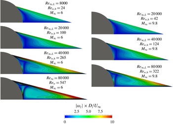
From figure 7, at a wake Reynolds number of 24 (
 $M_{\infty }=6$
,
 $Re_{\infty ,L}=8\times 10^{3}$
) the wake is clearly diffusion dominated. The role of convection on the vorticity distribution is negligible. The vorticity contours indicate a constant diffusive flux of vorticity between the opposing streams. At
 $Re_{w,h}=100$
, the convection of vorticity by the recirculating streamlines can start to be seen. However, the importance of diffusion in the wake is still evident. At a wake Reynolds number of 265 (
 $M_{\infty }=6$
,
 $Re_{\infty ,L}=4\times 10^{4}$
), convection is evident but the constant vorticity core is relatively small. At the wake Reynolds number of 547 (
 $M_{\infty }=6$
,
 $Re_{\infty ,L}=8\times 10^{4}$
) vorticity can clearly be seen convecting with the motion of the wake recirculation streamlines. At this Reynolds number, a small low strength secondary vortex has formed. These observations agree with the ranges presented by Grasso & Pettinelli (Reference Grasso and Pettinelli1995).
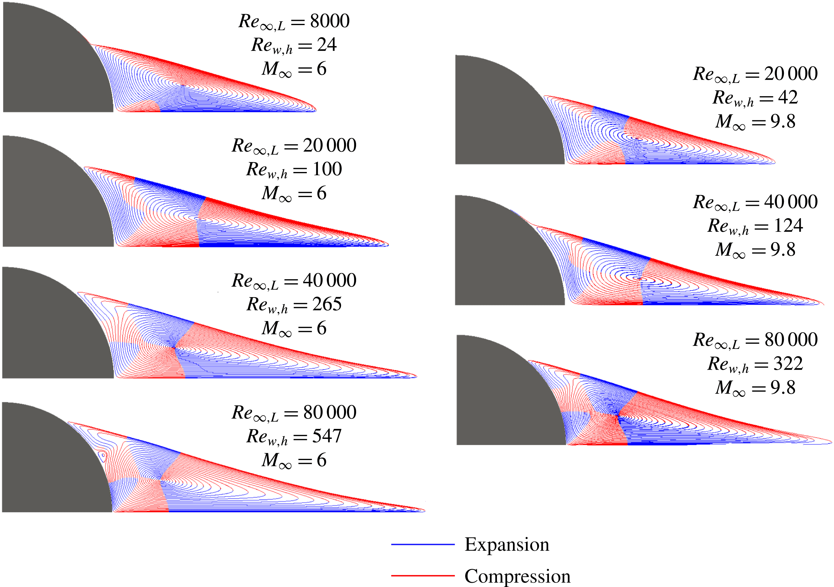
Regions of compression and expansion at various wake Reynolds numbers (planar wake).

Finite regions of compression and expansion are known to occur in the near wake and have an impact on the wake topology (Grasso & Pettinelli Reference Grasso and Pettinelli1995). These are also known to be a function of wake Reynolds number. In order to visualize this, the expansion and compression regions were extracted by taking the dot product of the local pressure gradient (
 $\unicode[STIX]{x1D735}p$
) with the local streamwise unit vector (
 ${\hat{s}}$
). In figure 8, the finite regions of compression and expansion are highlighted in red and blue, respectively. As the role of diffusion decreases (with increasing wake Reynolds number) these regions become more prominent. For example, at the wake Reynolds number of 24 the dividing streamline of the near wake experiences compression for its entire length. However, both compression and expansion are seen when lower diffusion is present.
Results at approximately Mach 10 are also included in figures 7 and 8. The observations and theoretical considerations presented in this section demonstrate that the state of the wake (diffusive or convective) and the observed topologies corresponding to that state are primarily a function of the pertinent wake Reynolds number. The wake Reynolds number has a nonlinear relationship to the free-stream Mach and Reynolds number. Due to compressibility and the presence of shocks, the characteristic wake Reynolds number is significantly smaller than the free-stream value. In many cases, a high Mach number flow can result in a laminar diffusion dominated wake even when the free-stream Reynolds number is high.
4 Analysis of wake mechanisms
In this section, analysis of the mechanisms in the hypersonic laminar near wake is performed incrementally. The observations made in this section form the ground work of the overall wake mechanism presented in § 5.
4.1 Control volume analysis of a planar wake
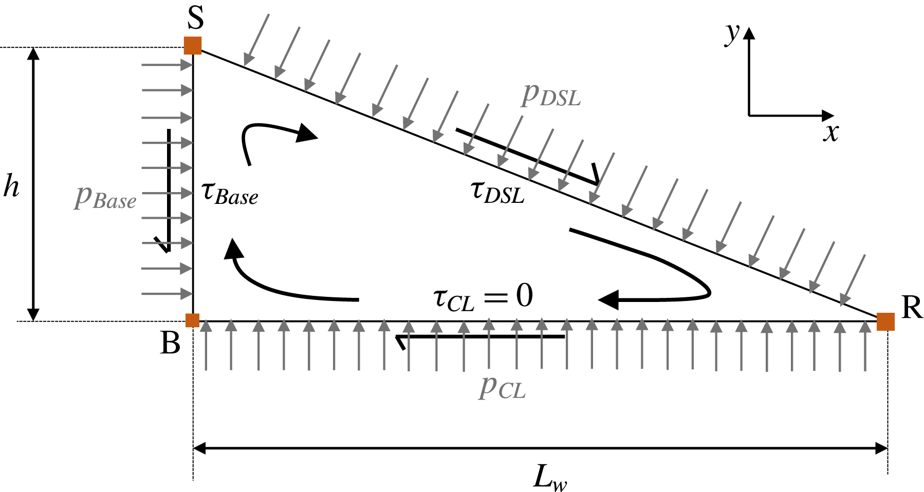
In order to begin analysing the near-wake recirculation feedback mechanism that joins the various interactions depicted in figure 1, a control volume analysis is used. Control volume (CV) analysis of the recirculation region is a simple yet powerful tool to demonstrate some of the observed near-wake relationships in terms of a simple force balance. The centreline, base, and dividing streamline enclose a system with no net mass transfer (and hence no convection) in or out. This means that the only terms appearing in an analysis of the volume are forces. Moreover, even though the dividing streamline and base surface have curvature, they can be approximated by the line segments shown in figure 9.
Control volume for recirculation region analysis.
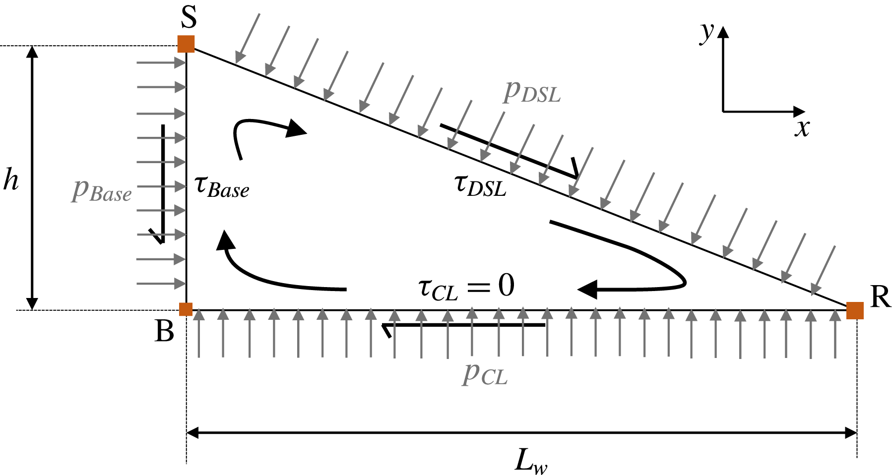
The force balances in the
 $x$
and
 $y$
directions from figure 9 can be rearranged for the ratio between wake length (
 $L_{w}$
) and wake base height (
 $h$
) yielding:
 $$\begin{eqnarray}\displaystyle & \displaystyle \frac{L_{w}}{h}=\frac{p_{DSL}-p_{Base}}{\unicode[STIX]{x1D70F}_{DSL}}=\frac{\unicode[STIX]{x1D70F}_{Base}+\unicode[STIX]{x1D70F}_{DSL}}{p_{CL}-p_{DSL}}. & \displaystyle\end{eqnarray}$$
From (4.1), several conclusions can be made regarding shear stress and pressures in the near wake. For a wake of finite size (
 $L_{w}/h$
or
 $h/L_{w}$
) to exist, it can be seen from (4.1) that
 $\unicode[STIX]{x1D70F}_{DSL}\neq 0$
. For
 $\unicode[STIX]{x1D70F}_{Base}$
(treated as positive in the
 $-y$
direction) the equation demonstrates that it cannot be equal and opposite to
 $\unicode[STIX]{x1D70F}_{DSL}$
. If it is assumed that the shear stress terms are always positive in the direction given in figure 9, it can be shown that for the above equation to hold the following inequality must be true:
 $$\begin{eqnarray}\displaystyle & \displaystyle p_{CL}>p_{DSL}>p_{Base}. & \displaystyle\end{eqnarray}$$
Given that the pressure is non-uniform along the CV boundaries, it is non-physical to assume a constant pressure recirculation region, which is often done in simple analyses (Chapman Reference Chapman1950; Delery & Lacau Reference Delery and Lacau1988). Regardless of
 $L_{w}/h$
, the mean centreline pressure must be greater than both the dividing streamline and the base. Additionally, the mean dividing streamline pressure must be greater than the base pressure.
To take this further, it is helpful to approximate the pressure along the each side of the control volume as the average of its endpoints. This is equivalent to assuming that the pressure varies linearly along each streamline. While this is not strictly true, it is useful for discussion and will be scrutinized in the following section. The approximations of the average streamline pressures are:
 $$\begin{eqnarray}\displaystyle & \displaystyle p_{CL}\approx \frac{p_{R}+p_{B}}{2}, & \displaystyle\end{eqnarray}$$
 $$\begin{eqnarray}\displaystyle & \displaystyle p_{DSL}\approx \frac{p_{R}+p_{S}}{2}, & \displaystyle\end{eqnarray}$$
 $$\begin{eqnarray}\displaystyle & \displaystyle p_{Base}\approx \frac{p_{S}+p_{B}}{2}. & \displaystyle\end{eqnarray}$$
By combining these approximations with the inequality in (4.2) and simplifying, it can be shown that
 $p_{B}>p_{S}$
,
 $p_{R}>p_{B}$
, and
 $p_{R}>p_{S}$
. These can be combined to produce the following inequality:
 $$\begin{eqnarray}\displaystyle & \displaystyle p_{R}>p_{B}>p_{S}. & \displaystyle\end{eqnarray}$$
This conclusion agrees well with conventional observation of the separation interaction that show that
 $p_{B}>p_{S}$
(Hinman & Johansen Reference Hinman and Johansen2016c
). Therefore, the highest pressure in the near wake must be at the reattachment point. Because at each streamline end point the static and stagnation pressures are equal (i.e.
 $p=p_{o}$
), these observations also lead to the inequality for streamline stagnation pressures:
 $$\begin{eqnarray}\displaystyle & \displaystyle p_{o,R}>p_{o,B}>p_{o,S}. & \displaystyle\end{eqnarray}$$
Additionally, applying the streamline pressure approximations (4.3) to (4.5) directly to the force balance in (4.1) yields:
 $$\begin{eqnarray}\displaystyle & \displaystyle \frac{L_{w}}{h}\approx \frac{p_{R}-p_{B}}{2\unicode[STIX]{x1D70F}_{DSL}}\approx \frac{2\left(\unicode[STIX]{x1D70F}_{Base}+\unicode[STIX]{x1D70F}_{DSL}\right)}{p_{B}-p_{S}}. & \displaystyle\end{eqnarray}$$
From this approximation it can be concluded that the base pressure and separation pressure cannot be equal. This is not a surprise because of the well-known lip-shock formation process. A more interesting observation is that the ratio between the length and height of the near wake can be approximately understood as the ratio between pressures and shear stress in the wake. Since
 $p_{B}-p_{S}$
consists partly of the lip-shock pressure rise, an explicit connection between separation and reattachment shocks via near-wake pressure, shear stress, and size is illustrated. For a given wake size (
 $L_{w}/h$
) a stronger recompression shock (corresponding to a higher
 $p_{R}-p_{B}$
) must correlate to a higher shear stress along the dividing streamline. This would also require an increase in lip-shock strength (
 $p_{B}-p_{S}$
). Similarly under a constant shear stress, an increase in
 $L_{w}/h$
indicates a decrease in lip-shock strength (
 $p_{B}-p_{S}$
) and an increase in reattachment pressure rise (
 $p_{R}-p_{B}$
). These hypotheses agree with conventional observations of wake Reynolds number dependence where
 $L_{w}/h$
increases with Reynolds number and the pressure rise at reattachment increases, and the pressure rise at the base is decreased.
4.2 Streamline pressures
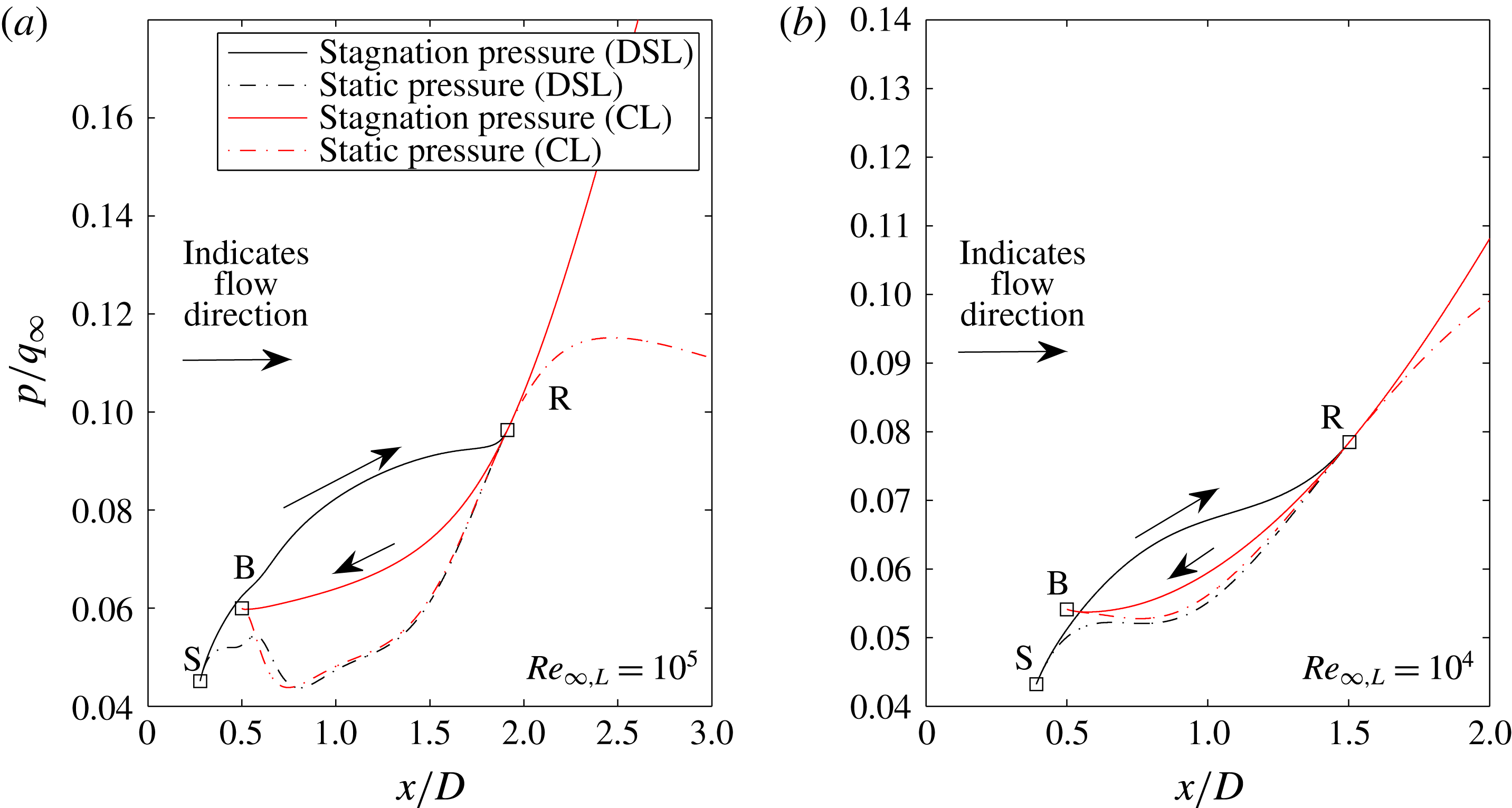
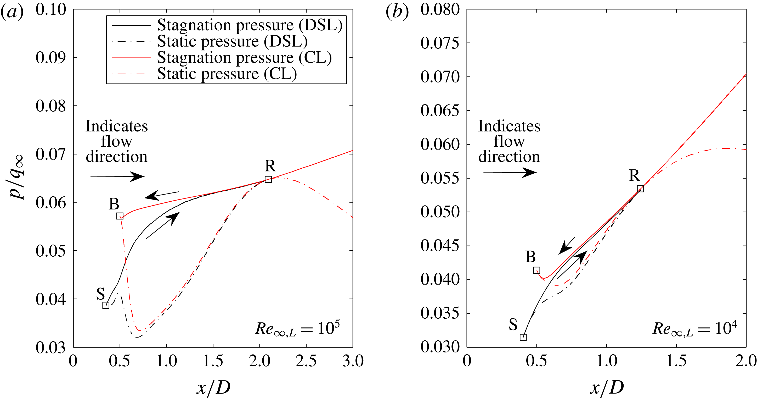
In the control volume analysis, conclusions and general requirements were presented for the pressure along the wake streamlines. Here, simulation results are used to further discuss these conclusions. The static and stagnation pressures have been extracted from the simulation results at
 $M_{\infty }=6$
,
 $Re_{\infty ,L}=10^{4}$
and
 $Re_{\infty ,L}=10^{5}$
for both an adiabatic sphere and cylinder. The pressures were found by tracing an approximate dividing streamline from the separation point to the reattachment point. Stagnation pressure was calculated by first using the NASA polynomials for total enthalpy to calculate total enthalpy and stagnation temperature. Then stagnation pressure was calculated from the stagnation temperature ratio and the isentropic equations. The pressures are plotted versus a normalized
 $x$
coordinate in figures 10 and 11.
Static and stagnation pressures along the near-wake streamlines (a)
 $Re=10^{5}$
(b)
 $Re=10^{4}$
(planar wake).

Static and stagnation pressures along the near-wake streamlines (a)
 $Re=10^{5}$
(b)
 $Re=10^{4}$
(axisymmetric wake).
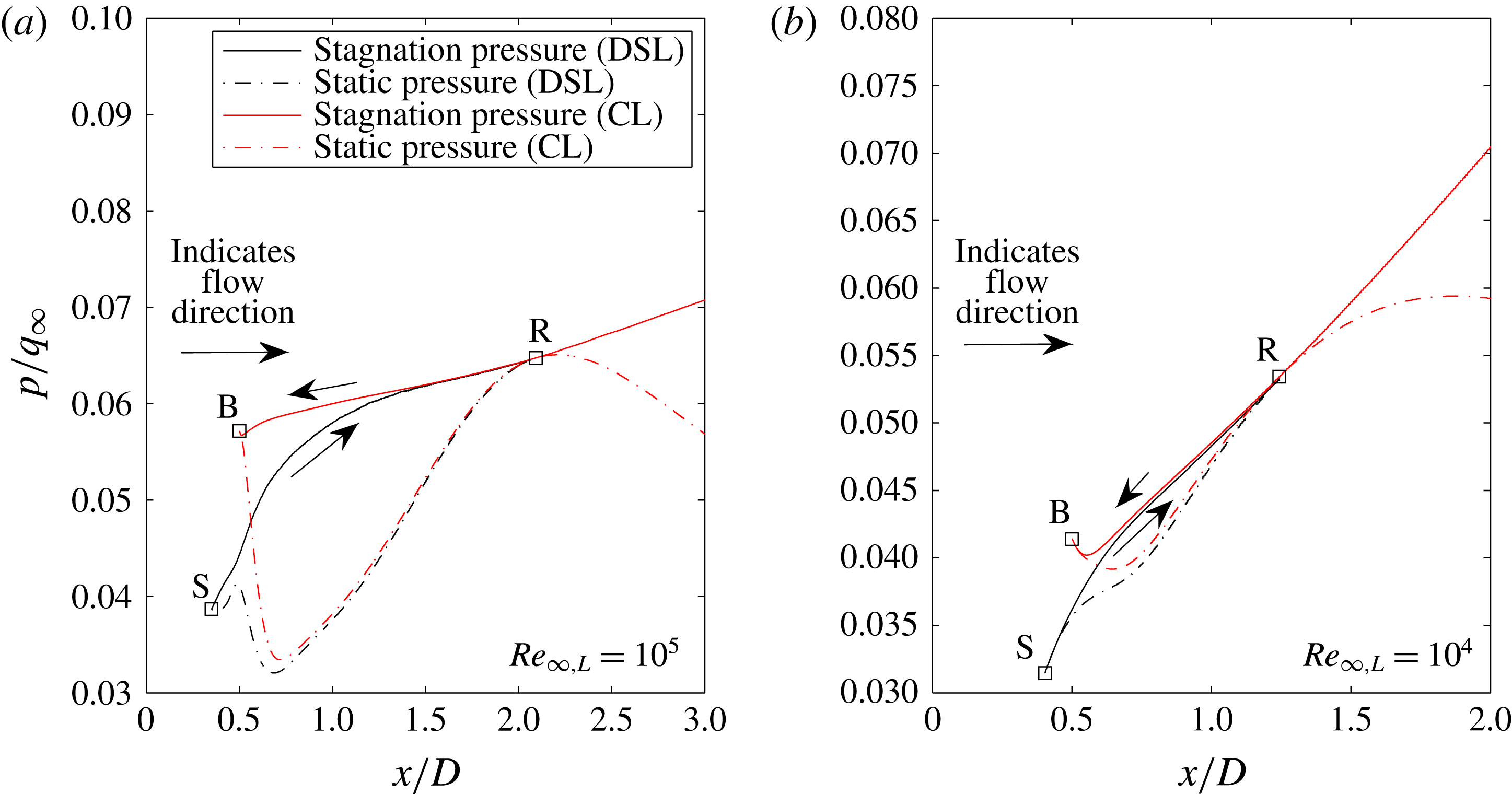
From the results, it is clear that the assumption of a linear pressure variation along the streamlines in the previous section is not valid. The static pressure both increases and decreases along each streamline length. However, the predicted relationships from (4.6) and (4.7) are still observed. At both Reynolds number conditions, the maximum pressure location within the near-wake recirculation region is at the reattachment point. At the lower Reynolds number, the variation of the static pressure along the streamline is greatly reduced. Thus at high Reynolds number diffusion plays a smaller role and the local static pressure is strongly driven by local changes in velocity and Mach number. This agrees with the observed differences between topology regimes A and C described in § 3 where finite regions of compression and expansion were observed as local wake Reynolds number was increased.
Stagnation pressure increases along the length of the dividing streamline. The mechanism of ‘division’ as the dividing streamline approaches the reattachment point is stagnation pressure deficiency of the inner streamlines. Thus, the mechanism by which this dividing stagnation pressure is achieved is crucial. A major assumption in the Chapman (Reference Chapman1950) type of analyses is that the dividing streamline is accelerated up to a similarity value and subsequently decelerated in an isentropic fashion. If this were the case, the results would show a stagnation pressure that increased up to a constant value that remains constant to reattachment. Instead, the results indicate that there is a continuous increase in stagnation pressure and therefore the isentropic relations based on a constant stagnation pressure are not valid. This alone does not indicate that the streamline is not isentropic however. This is further investigated in the wake streamline equation analysis.
Along the centreline the stagnation pressure decreases between the wake reattachment point and the rear-stagnation point. Conversely, the static pressure decreases from reattachment and then increases as the flow stagnates at the base. In the direct vicinity of the base (close to B) the results show that at both high and low Reynolds number a significant variation of pressure exists between the centreline and the dividing streamline. This indicates that an integral or thin-layer-type analysis of this section of the flow will be in error. However, downstream of the immediate aft-body the vertical pressure variation is small for both high and low Reynolds number. This observation indicates that in these regions a one-dimensional or integral approach with a family of wake profiles (such as Crocco & Lees (Reference Crocco and Lees1952) type analysis) is appropriate.
4.3 Wake streamline equation analysis
To analyse the mechanism by which the wake streamlines gain and lose pressure, and thereby link the reattachment and lip shocks, the governing equations are analysed along the enclosing boundaries: the dividing streamline, the wake centreline and the base.
4.3.1 Streamwise momentum equation
The steady-state momentum equation in the streamwise direction can be represented as the dot product of the conservative Navier–Stokes momentum equation with the streamwise unit vector,
 ${\hat{s}}$
:
 $$\begin{eqnarray}\displaystyle & \displaystyle \left[\unicode[STIX]{x1D735}\boldsymbol{\cdot }\left[\boldsymbol{V}\left(\unicode[STIX]{x1D70C}\boldsymbol{V}\right)\right]\right]\boldsymbol{\cdot }{\hat{s}}+\left[\unicode[STIX]{x1D735}p\right]\boldsymbol{\cdot }{\hat{s}}=\left[\unicode[STIX]{x1D735}\boldsymbol{\cdot }\unicode[STIX]{x1D70F}\right]\boldsymbol{\cdot }{\hat{s}}, & \displaystyle\end{eqnarray}$$
 $$\begin{eqnarray}\displaystyle & \displaystyle {\hat{s}}=\frac{\boldsymbol{V}}{|\boldsymbol{V}|}. & \displaystyle\end{eqnarray}$$
In the case of the wall boundary on the base,
 ${\hat{s}}$
is the wall tangent unit vector. The length along a given boundary or streamline is denoted,
 $|s|$
. This equation is simplified through simple calculus and assumptions of the character of the flow. The pressure gradient is given by the gradient of pressure in the streamwise direction. By assuming that the velocity field dilatation (
 $\unicode[STIX]{x1D735}\boldsymbol{\cdot }\boldsymbol{V}$
) is negligible in the wake region, and that the normal viscous stress components
 $\unicode[STIX]{x1D70F}_{ii}$
are negligible, the overall viscous stress term of the equation can be modified to be a function of vorticity. This becomes useful later when the discussion of the recirculation region as a vorticity sink is presented. The simplified form of the momentum equation in the
 ${\hat{s}}$
direction for planar flow is:
 $$\begin{eqnarray}\displaystyle & \displaystyle \frac{\unicode[STIX]{x2202}\unicode[STIX]{x1D70C}u_{{\hat{s}}}^{2}}{\unicode[STIX]{x2202}{\hat{s}}}+\frac{\unicode[STIX]{x2202}\unicode[STIX]{x1D70C}u_{{\hat{s}}}u_{\hat{n}}}{\unicode[STIX]{x2202}\hat{n}}+\frac{\unicode[STIX]{x2202}p}{\unicode[STIX]{x2202}{\hat{s}}}=-\frac{\unicode[STIX]{x2202}}{\unicode[STIX]{x2202}\hat{n}}\left(\unicode[STIX]{x1D707}\unicode[STIX]{x1D714}_{z}\right). & \displaystyle\end{eqnarray}$$
For the adiabatic case, the viscous term can be simplified further. Since the wake is adiabatic in the cases examined here, then it is assumed
 $\unicode[STIX]{x2202}T/\unicode[STIX]{x2202}\hat{n}$
is relatively small along dividing streamline and by extension
 $(\unicode[STIX]{x2202}\unicode[STIX]{x1D707})/(\unicode[STIX]{x2202}\hat{n})$
is negligible. Therefore, for the present analysis, the simplified form of the streamwise momentum equation is given by:
 $$\begin{eqnarray}\displaystyle & \displaystyle \frac{\unicode[STIX]{x2202}\unicode[STIX]{x1D70C}u_{{\hat{s}}}^{2}}{\unicode[STIX]{x2202}{\hat{s}}}+\frac{\unicode[STIX]{x2202}\unicode[STIX]{x1D70C}u_{{\hat{s}}}u_{\hat{n}}}{\unicode[STIX]{x2202}\hat{n}}+\frac{\unicode[STIX]{x2202}p}{\unicode[STIX]{x2202}{\hat{s}}}=-\unicode[STIX]{x1D707}\frac{\unicode[STIX]{x2202}\unicode[STIX]{x1D714}_{z}}{\unicode[STIX]{x2202}\hat{n}}. & \displaystyle\end{eqnarray}$$
The contribution of the viscous term on the right-hand side of the equation will be referred to as viscous vorticity flux. This flux occurs across streamlines or is vorticity production at the wall due to the pressure gradient. Equation (4.12) is valid for both the dividing streamline and the centreline in two-dimensional flow. Along the base, the advective terms are zero. In the axisymmetric case, the equation must be modified. The equation for the conservation of linear momentum along the dividing streamline generalized for both two-dimensional (2-D) planar and 2-D axisymmetric wake flows is given by:
 $$\begin{eqnarray}\displaystyle & \displaystyle \frac{\unicode[STIX]{x2202}\unicode[STIX]{x1D70C}u_{{\hat{s}}}^{2}}{\unicode[STIX]{x2202}{\hat{s}}}+\frac{\unicode[STIX]{x2202}\unicode[STIX]{x1D70C}u_{{\hat{s}}}u_{\hat{n}}}{\unicode[STIX]{x2202}\hat{n}}+b\frac{\unicode[STIX]{x2202}\unicode[STIX]{x1D70C}u_{{\hat{s}}}u_{\hat{z}}}{\unicode[STIX]{x2202}\hat{z}}+\frac{\unicode[STIX]{x2202}p}{\unicode[STIX]{x2202}{\hat{s}}}=-\unicode[STIX]{x1D707}\frac{\unicode[STIX]{x2202}\unicode[STIX]{x1D714}_{\hat{z}}}{\unicode[STIX]{x2202}\hat{n}}-\unicode[STIX]{x1D707}b\left(\frac{\unicode[STIX]{x1D714}_{\hat{z}}}{y}\right)\hat{n}_{y}. & \displaystyle\end{eqnarray}$$
Here,
 $b=0$
for two dimensions,
 $b=1$
for axisymmetry and
 $y$
is the local distance to the streamline from the axis of symmetry.
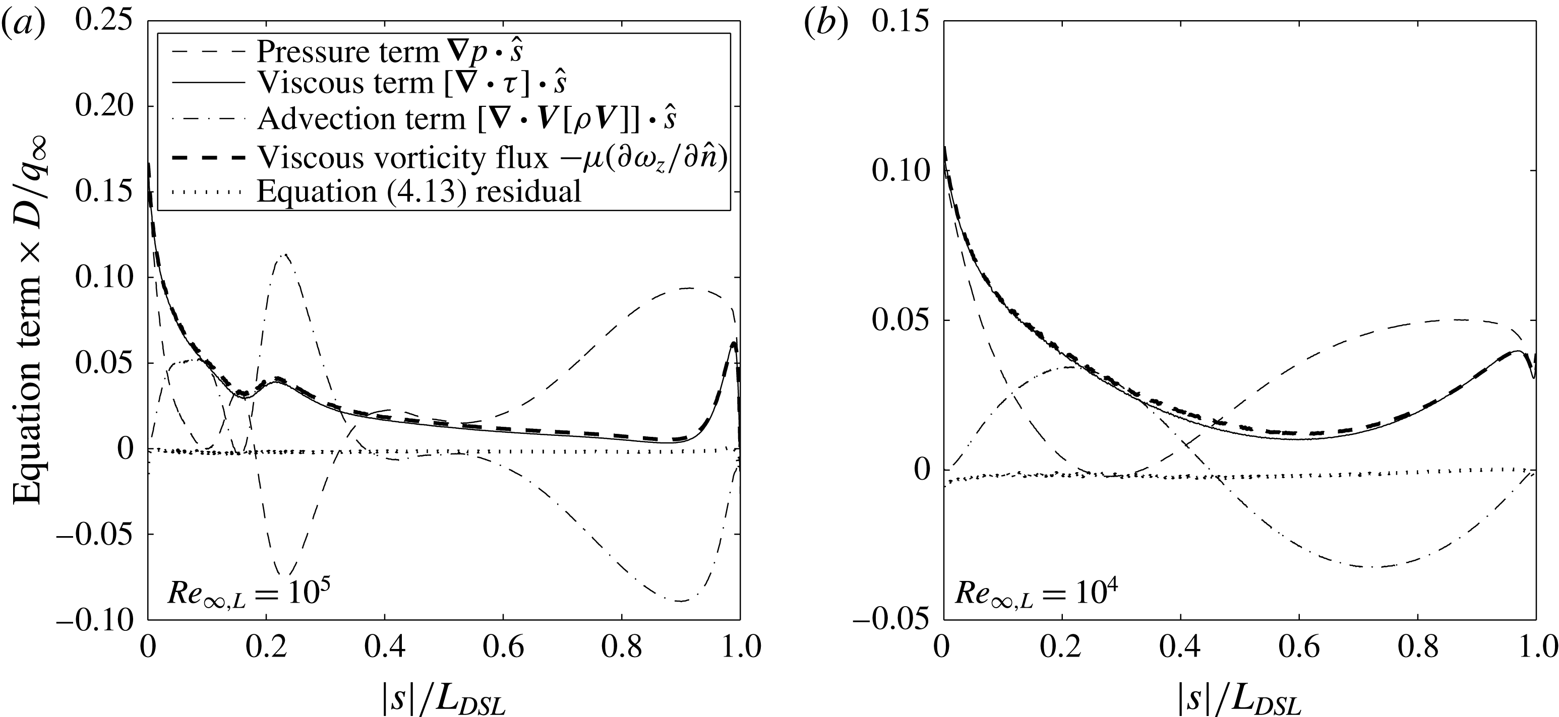
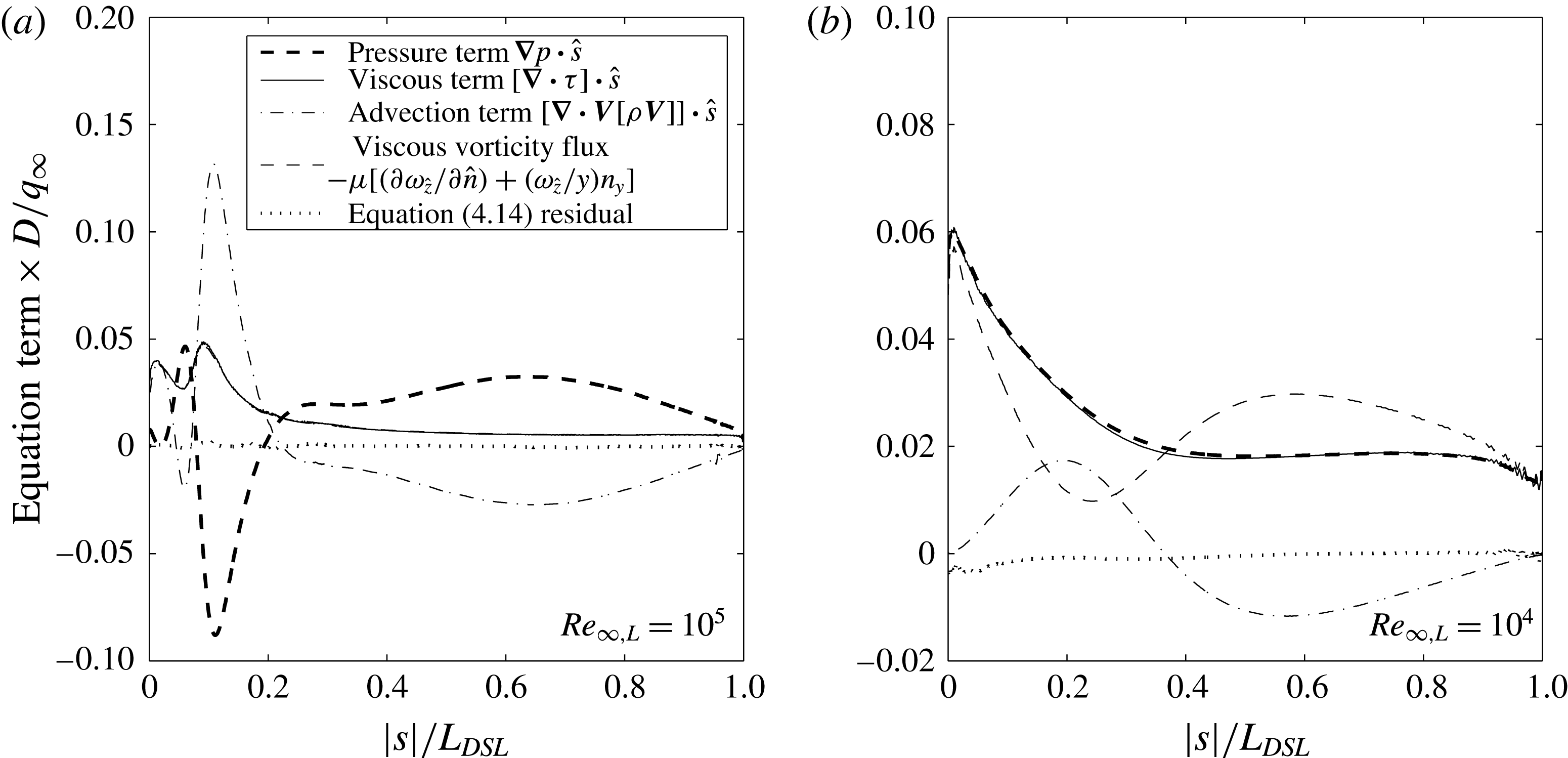
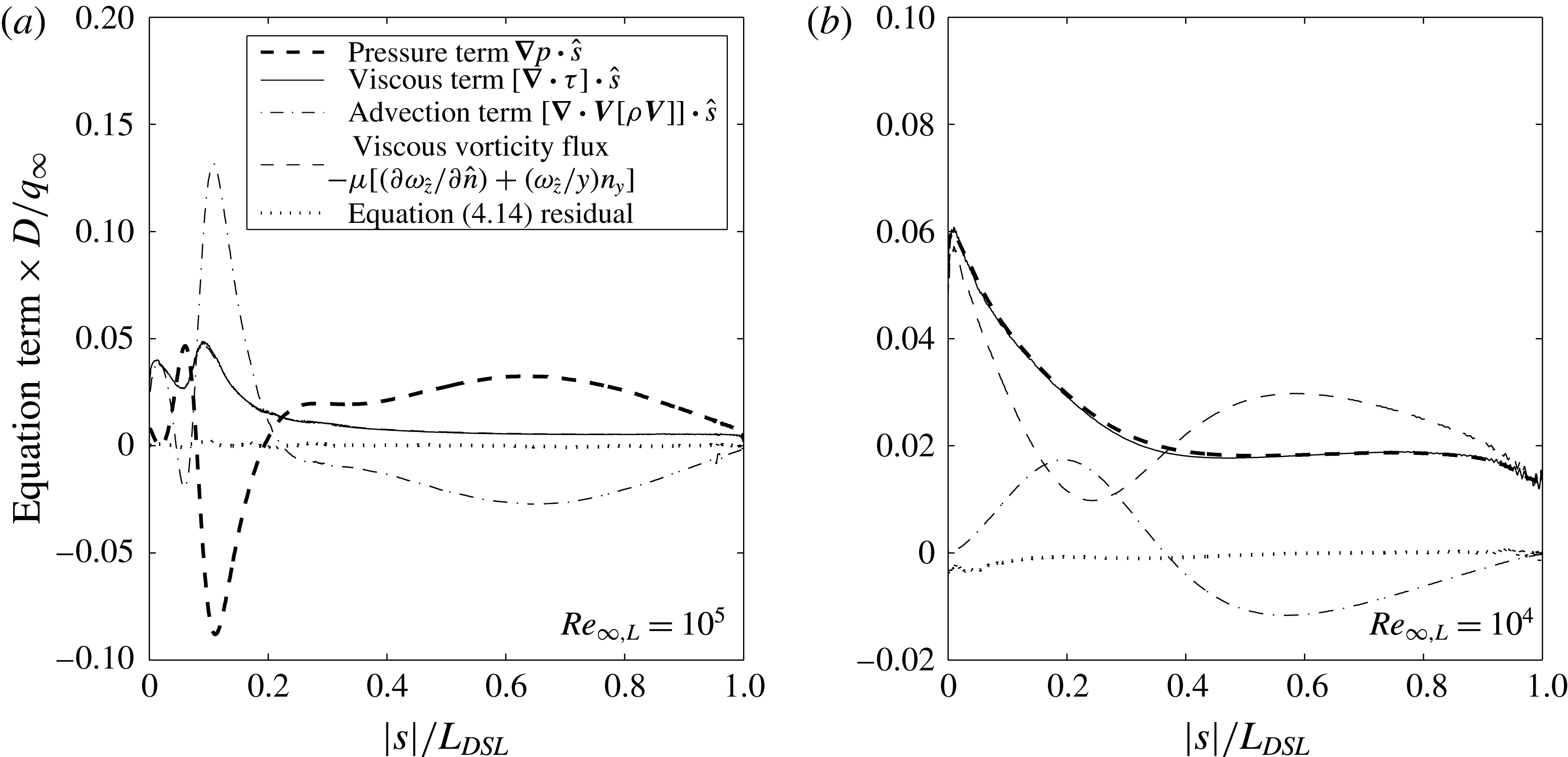
Terms of the streamwise equation of linear momentum (dividing streamline – planar wake).

The wake centreline has a slightly modified form:
 $$\begin{eqnarray}\displaystyle & \displaystyle \frac{\unicode[STIX]{x2202}\unicode[STIX]{x1D70C}u_{{\hat{s}}}^{2}}{\unicode[STIX]{x2202}{\hat{s}}}+\frac{\unicode[STIX]{x2202}\unicode[STIX]{x1D70C}u_{{\hat{s}}}u_{\hat{n}}}{\unicode[STIX]{x2202}\hat{n}}+b\frac{\unicode[STIX]{x2202}\unicode[STIX]{x1D70C}u_{{\hat{s}}}u_{\hat{z}}}{\unicode[STIX]{x2202}\hat{z}}+\frac{\unicode[STIX]{x2202}p}{\unicode[STIX]{x2202}{\hat{s}}}=-\left(b+1\right)\unicode[STIX]{x1D707}\frac{\unicode[STIX]{x2202}\unicode[STIX]{x1D714}_{z}}{\unicode[STIX]{x2202}\hat{n}}. & \displaystyle\end{eqnarray}$$
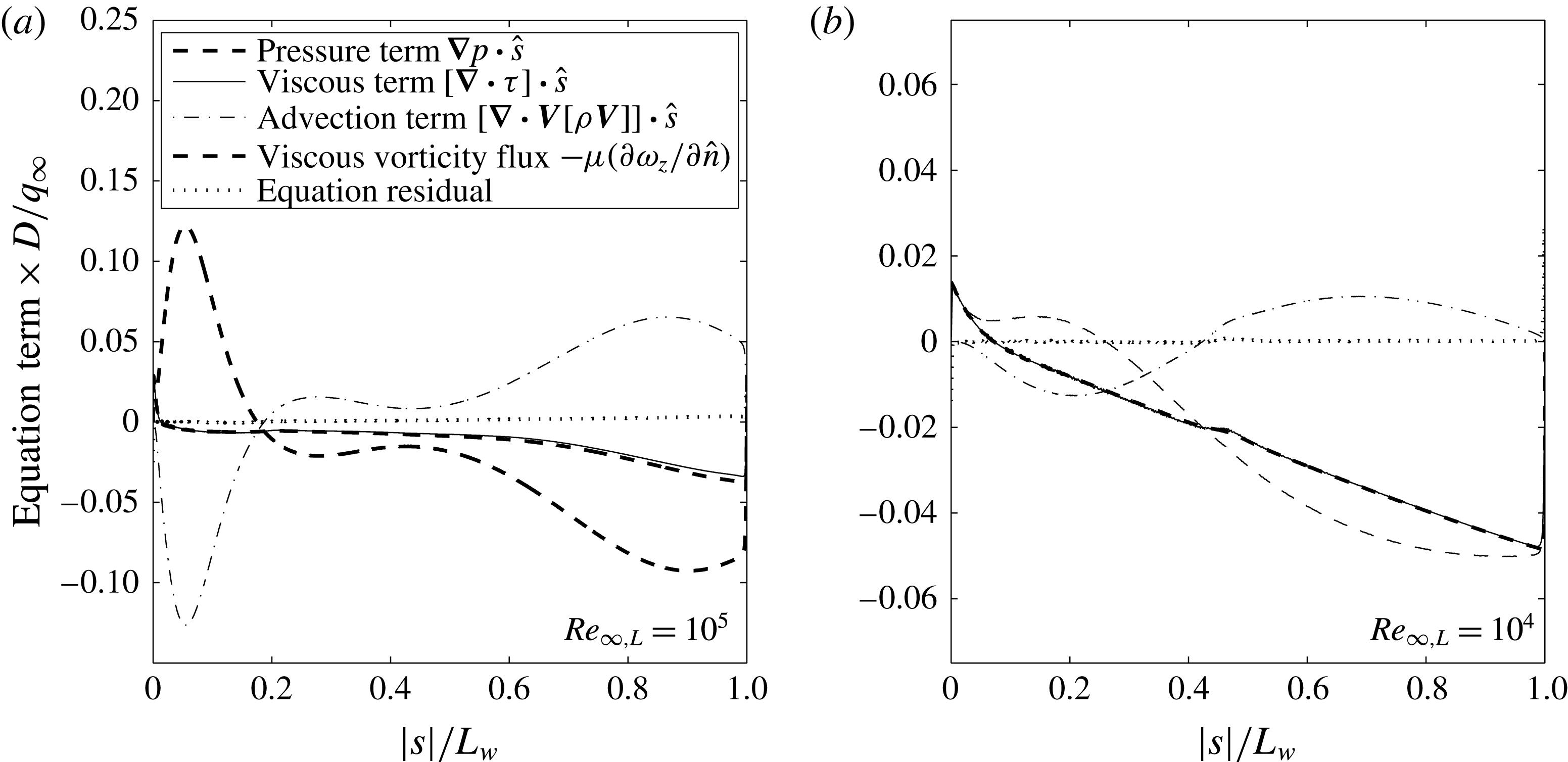
To assess the validity of these assumptions as well as examine the relative magnitudes of these terms, the individual terms from (4.12) are examined along the streamlines enclosing the recirculation region (the dividing streamline and the centreline) for the 2-D case. These terms are plotted along the dividing streamline for two representative Reynolds numbers (
 $Re_{\infty ,L}=10^{5}$
and
 $Re_{\infty ,L}=10^{4}$
) in figure 12. The residual from (4.12) is also shown. The results show that the actual divergence of the shear stress tensor is close to the approximation of this term as viscous vorticity flux. There is some odd behaviour in the figure close to the separation and reattachment points. This is due to the fact that the streamwise unit vector,
 ${\hat{s}}$
is poorly defined near these points, making calculation in the vicinity of stagnation difficult and at stagnation impossible. In addition to the dividing streamline in the planar case, the terms along the dividing streamline in axisymmetric flow are plotted in figure 13 (again for
 $Re_{\infty ,L}=10^{5}$
and
 $Re_{\infty ,L}=10^{4}$
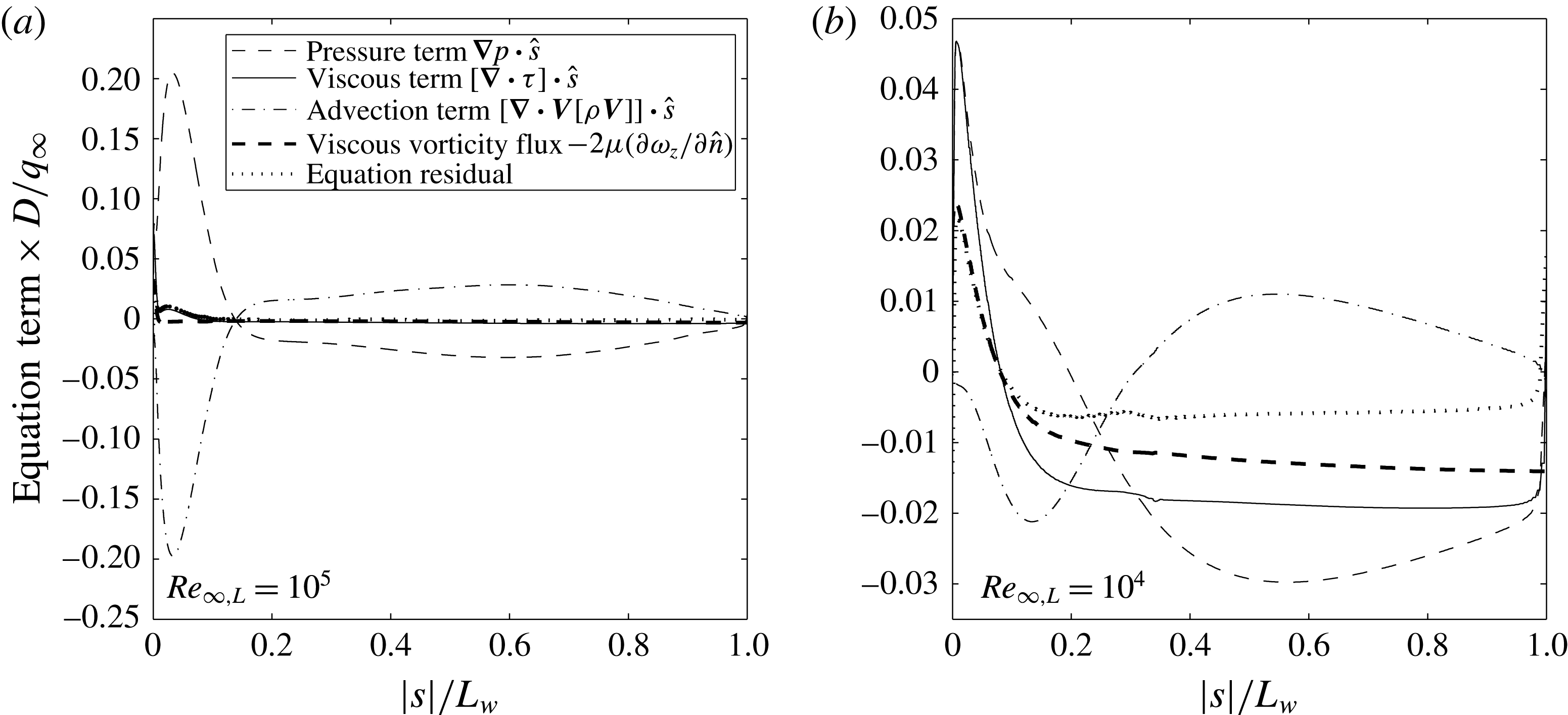
). For both axisymmetric and planar wake flow, the primary mechanism along the dividing streamline is viscous vorticity flux. In figures 14 and 15, the streamwise momentum terms are plotted. Along the axisymmetric wake centreline the results show that the viscous vorticity flux term is not a good approximation for the divergence of the viscous stress tensor. However, the viscous stress term, in general, is less dominant with the exception of low Reynolds number cases.
Terms of the streamwise equation of linear momentum (dividing streamline – axisymmetric wake).
Terms of the streamwise equation of linear momentum (centreline – planar wake).

Terms of the streamwise equation of linear momentum (centreline – axisymmetric).

The term-by-term analysis of the streamwise momentum equations shown in figures 12 to 15 can be used to highlight the pertinent mechanisms along the length of each streamline. In the low Reynolds number case, the pressure gradient along the dividing streamline is never negative. Additionally, it is clear that the vorticity flux term is dominant along the streamline. Conversely, in the high Reynolds number case there are distinct regions of positive and negative pressure gradient. The near mirroring of the advective term with the pressure gradient in these regions demonstrates the reduced importance of the viscous vorticity flux as Reynolds number is increased. This is consistent with the observed regions of compression and expansion in figure 7. Another observation is the change of sign in viscous vorticity flux close to the base on the centreline. This is consistent with planar stagnation point flow where a gain in stagnation pressure is observed as viscous flow stagnates (Schlichting Reference Schlichting1979).
4.3.2 Streamline momentum accounting - planar wake
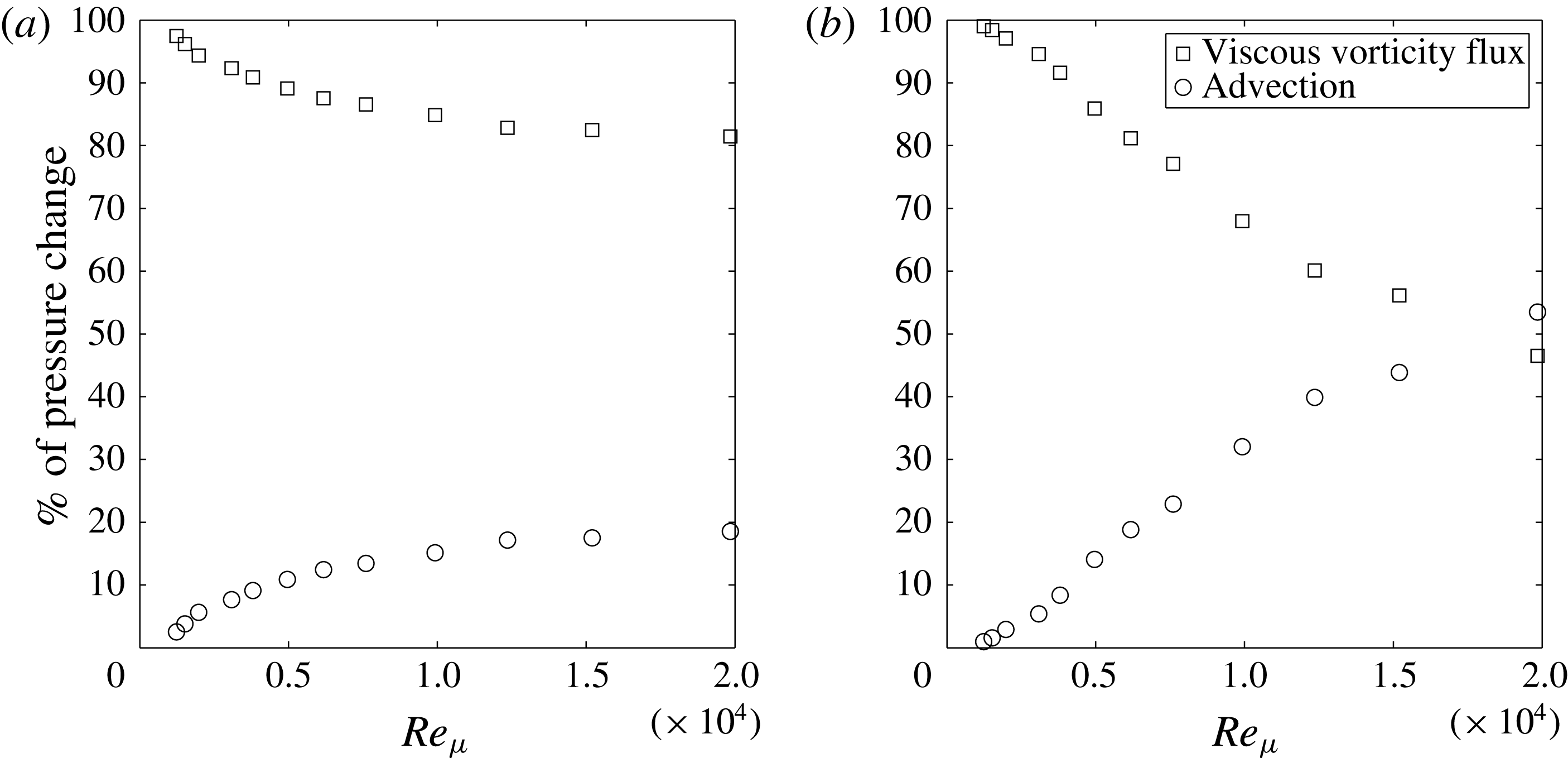
Integration of the momentum equation can be used to illustrate the proportion of stagnation pressure change due to the vorticity flux and the advection term. Equation (4.12) is integrated along the dividing streamline (S to R) and the wake centreline (R to B) in the planar case. The integrated equations are:
 $$\begin{eqnarray}\displaystyle & \displaystyle p_{R}-p_{S}=p_{o,R}-p_{o,S}=-\int _{S}^{R}\unicode[STIX]{x1D707}\frac{\unicode[STIX]{x2202}\unicode[STIX]{x1D714}_{z}}{\unicode[STIX]{x2202}\hat{n}}\,\text{d}{\hat{s}}-\int _{S}^{R}\unicode[STIX]{x1D70C}u_{{\hat{s}}}\frac{\unicode[STIX]{x2202}u_{{\hat{s}}}}{\unicode[STIX]{x2202}{\hat{s}}}\,\text{d}{\hat{s}}, & \displaystyle\end{eqnarray}$$
 $$\begin{eqnarray}\displaystyle & \displaystyle p_{B}-p_{R}=p_{o,B}-p_{o,R}=-\int _{R}^{B}\unicode[STIX]{x1D707}\frac{\unicode[STIX]{x2202}\unicode[STIX]{x1D714}_{z}}{\unicode[STIX]{x2202}\hat{n}}\,\text{d}{\hat{s}}-\int _{R}^{B}\unicode[STIX]{x1D70C}u_{{\hat{s}}}\frac{\unicode[STIX]{x2202}u_{{\hat{s}}}}{\unicode[STIX]{x2202}{\hat{s}}}\,\text{d}{\hat{s}}. & \displaystyle\end{eqnarray}$$
In incompressible flow, the advection terms in (4.15) and (4.16) would be conservative when integrating between two stagnation points. However, in compressible flow the density is subject to change along the length of the streamline. Thus, due to compressibility, this term cannot be ignored and is a fundamental part of the stagnation pressure gain along the streamline. The maximum Mach number along the dividing streamline in the cases examined is approximately
 $0.8$
.
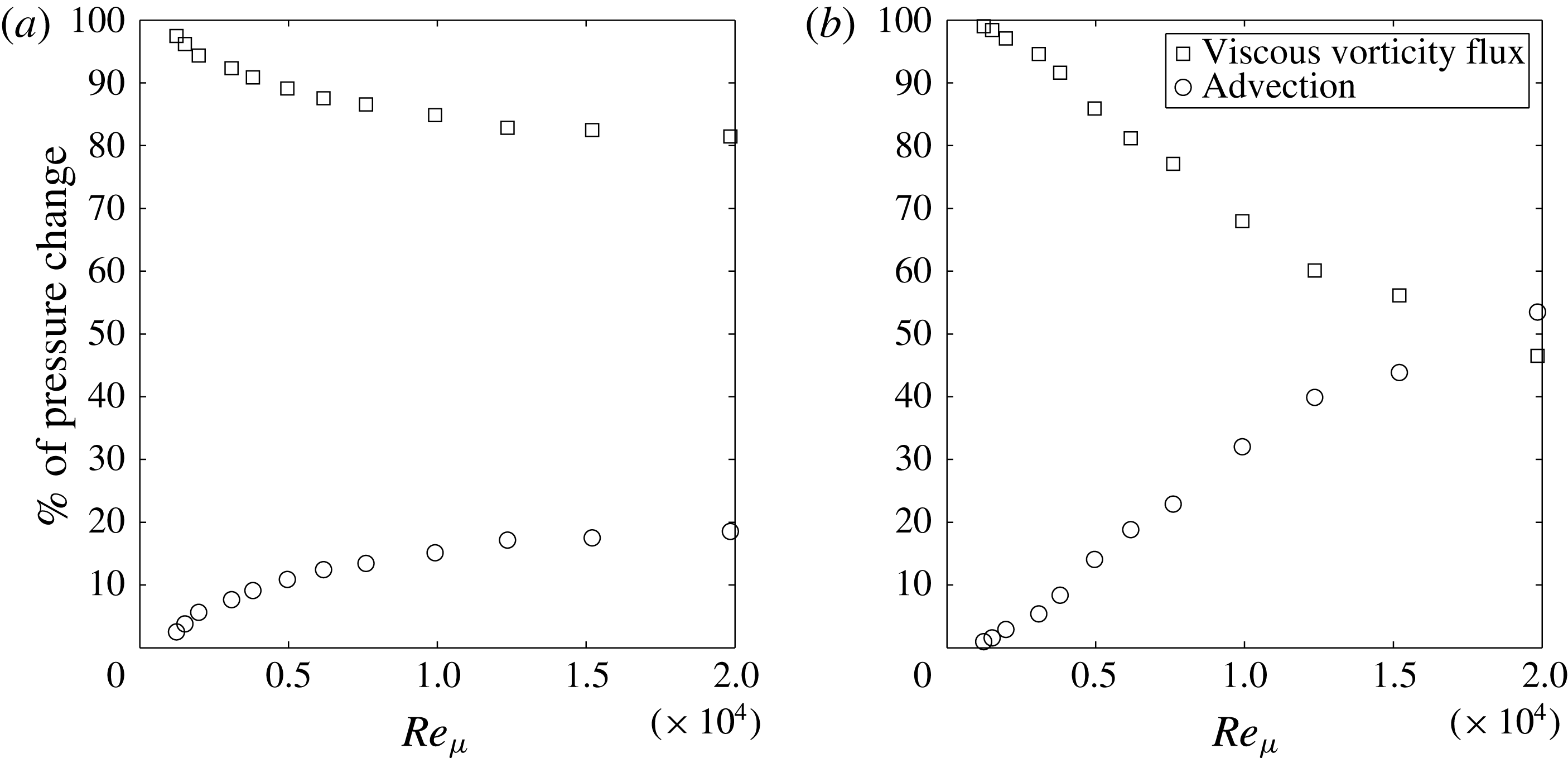
The accounting of the changes in wake streamline stagnation pressure found from the simulation data are given in figure 16. At low Reynolds number, along the dividing streamline it is clear that the mechanism of stagnation pressure gain is primarily the viscous vorticity flux across it. At both low and high Reynolds number, viscous vorticity flux dominates the accounting of stagnation pressure gain. The centreline, however, shows a strong dependence on Reynolds number. At high Reynolds number, the stagnation pressure loss due to the advection equation is significant. Referring back to figure 14, it can be seen that the viscous vorticity flux is of a similar magnitude to advection at high Reynolds number whereas at low Reynolds number the viscous vorticity flux is dominant.
Momentum equation streamline accounting – dividing streamline (a) and centreline (b) – planar wake.
4.3.3 Vorticity equation - planar wake
The preceding examination of the streamline momentum equation indicates that a major mechanism along the streamline is viscous vorticity flux. It was shown that viscous vorticity flux is a good approximation for the diffusion of momentum. As well, the process of streamline accounting indicated that this is the primary mechanism of stagnation pressure gain along the dividing streamline. In order to better examine the mechanism of vorticity transfer across the streamlines, it is useful to examine the two-dimensional vorticity equation. Since there is no mass flow in or out of the near-wake recirculation region, it is clear that the mechanism driving the vorticity flux is diffusion. However, through examination of the vorticity equation (assuming planar incompressible flow to illustrate) along a streamline this can be more rigorously shown:
 $$\begin{eqnarray}\displaystyle & \displaystyle \unicode[STIX]{x1D70C}u_{s}\frac{\unicode[STIX]{x2202}\unicode[STIX]{x1D714}_{\hat{z}}}{\unicode[STIX]{x2202}{\hat{s}}}+\unicode[STIX]{x1D70C}u_{\hat{n}}\frac{\unicode[STIX]{x2202}\unicode[STIX]{x1D714}_{\hat{z}}}{\unicode[STIX]{x2202}\hat{n}}=\unicode[STIX]{x1D707}\left(\frac{\unicode[STIX]{x2202}^{2}\unicode[STIX]{x1D714}_{\hat{z}}}{\unicode[STIX]{x2202}\hat{n}^{2}}+\frac{\unicode[STIX]{x2202}^{2}\unicode[STIX]{x1D714}_{\hat{z}}}{\unicode[STIX]{x2202}{\hat{s}}^{2}}\right). & \displaystyle\end{eqnarray}$$
The simplest example is the planar centreline streamline. Along the centreline,
 $\unicode[STIX]{x1D714}_{\hat{z}}=0$
,
 $u_{\hat{n}}=0$
,
 $\unicode[STIX]{x2202}\unicode[STIX]{x1D714}_{\hat{z}}/\unicode[STIX]{x2202}{\hat{s}}$
and
 $\unicode[STIX]{x2202}^{2}\unicode[STIX]{x1D714}_{\hat{z}}/\unicode[STIX]{x2202}{\hat{s}}^{2}=0$
. Therefore the vorticity equation becomes:
 $$\begin{eqnarray}\displaystyle & \displaystyle \frac{\unicode[STIX]{x2202}^{2}\unicode[STIX]{x1D714}_{\hat{z}}}{\unicode[STIX]{x2202}\hat{n}^{2}}=0. & \displaystyle\end{eqnarray}$$
Thus the profile of vorticity gradient across the centreline is therefore always linear. By extension, since the vorticity must have opposite sign above and below the centreline, the centreline must behave as a vorticity sink. This is a condition that is always true for a symmetry plane. The counter-rotating vortices in the near wake are analogous to side-by-side regions of hot and cold fluids. The boundary between them is a sink to the vorticity magnitude on either side.
The dividing streamline is more complicated. Along the streamline, the velocity normal to the streamline is zero (
 $u_{\hat{n}}=0$
). Therefore along the dividing streamline, the vorticity equation becomes:
 $$\begin{eqnarray}\displaystyle & \displaystyle \unicode[STIX]{x1D70C}u_{{\hat{s}}}\frac{\unicode[STIX]{x2202}\unicode[STIX]{x1D714}_{\hat{z}}}{\unicode[STIX]{x2202}{\hat{s}}}=\unicode[STIX]{x1D707}\left(\frac{\unicode[STIX]{x2202}^{2}\unicode[STIX]{x1D714}_{\hat{z}}}{\unicode[STIX]{x2202}\hat{n}^{2}}+\frac{\unicode[STIX]{x2202}^{2}\unicode[STIX]{x1D714}_{\hat{z}}}{\unicode[STIX]{x2202}{\hat{s}}^{2}}\right). & \displaystyle\end{eqnarray}$$
Along the streamline, vorticity can be advected and/or diffused. However, since
 $u_{n}=0$
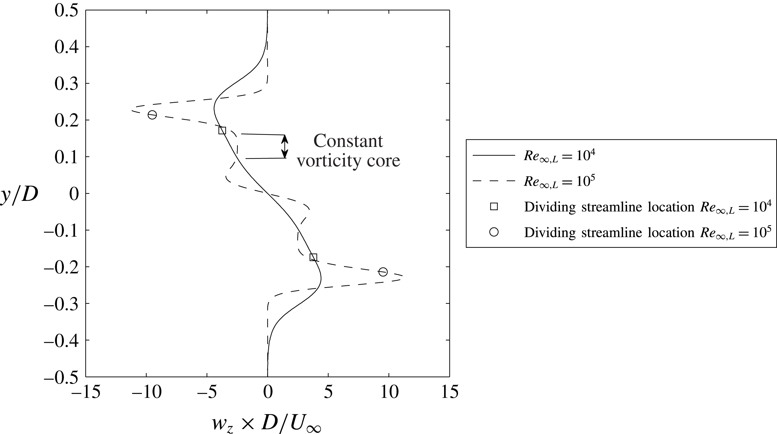
only diffusion can accomplish a flux of vorticity normal to the streamline. Overall, the wake acts as a sink of vorticity to the highly vortical outer layer of the wake shear layer. The peak in vorticity occurs outside the recirculation region and diffuses both outwards to the outer flow, and into the wake and across the dividing streamline. This is demonstrated by the vorticity profile through the centre of the wake as shown in figure 17. The profile was extracted along a vertical line at one cylinder radius downstream of the base. In order for the wake to maintain itself it must receive a constant supply of vorticity from the external stream. This vorticity is generated upstream of the wake on the body due to the favourable pressure gradient, through regions of the bow and lip-shock waves with curvature, and from regions with baroclinic torques. Therefore, the vorticity generation upstream of the wake is of fundamental importance to the wake physics. It was shown in previous work (Hinman & Johansen Reference Hinman and Johansen2016a
) that a viscous near wake could still form with slip wall boundaries on the body surface. In that case the wake was sustained by vorticity generated by baroclinic torques upstream of the wake.
Vorticity profile at
 $x=0.5D$
downstream from base – planar wake.
4.3.4 Energy and entropy equations - planar wake
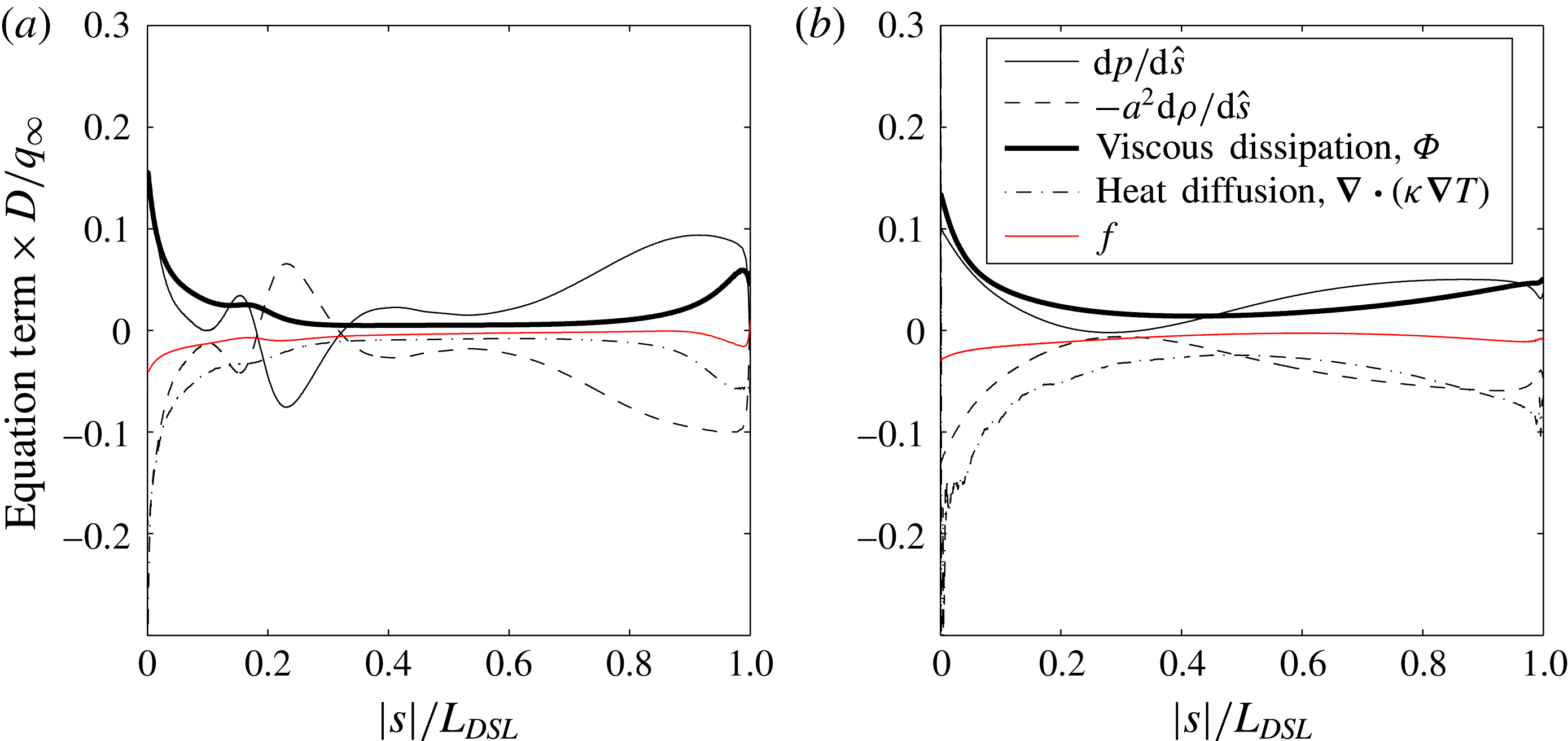
It has now been shown using control volume analysis, and through examination of simulation results, that there is a distinct stagnation pressure gain along the length of the dividing streamline. For flow problems, stagnation properties and entropy are closely linked by the second law of thermodynamics. For greater understanding, it is necessary to analyse this streamline further utilizing the energy equations and entropy equations. The energy equation (simplified by aligning with stream coordinate system) is:
 $$\begin{eqnarray}\displaystyle & \displaystyle \unicode[STIX]{x1D70C}u_{{\hat{s}}}\frac{\unicode[STIX]{x2202}h}{\unicode[STIX]{x2202}{\hat{s}}}=u_{{\hat{s}}}\frac{\unicode[STIX]{x2202}p}{\unicode[STIX]{x2202}{\hat{s}}}+\unicode[STIX]{x1D735}\boldsymbol{\cdot }\left(\unicode[STIX]{x1D705}\unicode[STIX]{x1D735}T\right)+\unicode[STIX]{x1D6F7}. & \displaystyle\end{eqnarray}$$
By multiplying the equation by
 $u_{{\hat{s}}}$
and performing some algebraic manipulation, the energy equation can be written in terms of the local pressure gradient in the streamline direction:
 $$\begin{eqnarray}\displaystyle & \displaystyle \frac{\unicode[STIX]{x2202}p}{\unicode[STIX]{x2202}{\hat{s}}}-a^{2}\frac{\unicode[STIX]{x2202}\unicode[STIX]{x1D70C}}{\unicode[STIX]{x2202}{\hat{s}}}=\frac{\unicode[STIX]{x1D6FE}-1}{u_{{\hat{s}}}}\left[\unicode[STIX]{x1D735}\boldsymbol{\cdot }\left(\unicode[STIX]{x1D705}\unicode[STIX]{x1D735}T\right)+\unicode[STIX]{x1D6F7}\right]=f. & \displaystyle\end{eqnarray}$$
By recognizing that when the speed of sound
 $a$
is equal to the isentropic wave speed, the left-hand side vanishes since in this case:
 $a^{2}=\unicode[STIX]{x2202}p/\unicode[STIX]{x2202}\unicode[STIX]{x1D70C}_{Isentropic}$
. Therefore, in the isentropic case both sides of (4.21) must equal zero. In the present analysis, the non-zero value of the left-hand side and right-hand side is represented by
 $f$
. The units of this equation are of the type
 $\unicode[STIX]{x0394}p/\unicode[STIX]{x0394}x$
and therefore the equation represents a non-isentropic contribution to the streamline pressure gradient. By examining the right-hand side of (4.21), it is seen that if the dividing streamline is compressed at constant entropy the viscous dissipation must be in direct balance with the heat transfer. This can also be shown utilizing the entropy transport equation. Assuming steady-state flow along a streamline:
 $$\begin{eqnarray}\displaystyle & \displaystyle \unicode[STIX]{x1D70C}u_{{\hat{s}}}\frac{\unicode[STIX]{x2202}s}{\unicode[STIX]{x2202}{\hat{s}}}=\frac{1}{T}\left[\unicode[STIX]{x1D735}\boldsymbol{\cdot }\left(\unicode[STIX]{x1D705}\unicode[STIX]{x1D735}T\right)+\unicode[STIX]{x1D6F7}\right]=\frac{u_{{\hat{s}}}}{T\left(\unicode[STIX]{x1D6FE}-1\right)}f. & \displaystyle\end{eqnarray}$$
Therefore, if the entropy increases or decreases along the dividing streamline then there is an imbalance between the entropy being generated by viscous dissipation and the entropy lost to diffusion. When
 $f<0$
entropy is being lost along the streamline, and conversely when
 $f>0$
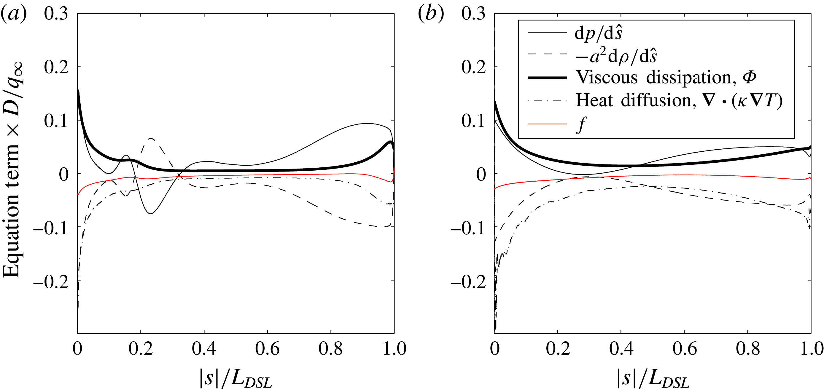
entropy is increasing. The terms of the energy equation, including the isentropic residual
 $f$
are plotted in figure 18. The profile of
 $f$
demonstrates that at both high and low Reynolds number there is a gradual decrease in entropy along the streamline. The viscous dissipation function by definition is always greater than zero. Therefore, the heat generated by viscous dissipation must be diffused away by the negative diffusion term
 $\unicode[STIX]{x1D735}\boldsymbol{\cdot }\left(\unicode[STIX]{x1D705}\unicode[STIX]{x1D735}T\right)$
. Since the residual
 $f$
, is less than zero along the dividing streamline the following process along the streamline is observed. While kinetic energy is being dissipated to heat, this process generates entropy through
 $\unicode[STIX]{x1D6F7}$
, however, faster than it is generated it is diffused to the surrounding flow. By this mechanism, the local entropy along the dividing streamline is decreased.
Terms of the energy equation (dividing streamline – planar wake).
This is in an important observation when compared with the classical treatment of the dividing streamline. In most early work, the compression of the dividing streamline was treated as isentropic (and constant stagnation pressure) (Delery & Lacau Reference Delery and Lacau1988). This facilitated easy calculation of base pressure through the Chapman similarity profile (Chapman Reference Chapman1950). Despite the ease of calculation, it was known that in fact the pressure reached due to the reattachment shock was much higher than the pressure reached by the dividing streamline, and that the dividing streamline was most likely not isentropic (Delery & Lacau Reference Delery and Lacau1988). This was accounted for by recovery factors representing the amount of downstream pressure recovered by the dividing streamline. This was purely empirical and the true nature of the dividing streamline has not been demonstrated. A common assumption is that the dividing streamline would be gaining entropy along its length, and this would result in a decrease of its stagnation pressure as it stagnated at reattachment.
4.4 Rear-stagnation point flow
Another observed mechanism within the near wake begins to occur as the diffusivity in the wake begins to reduce (topology regime B). As the centreline flow approaches the base it undergoes a viscous planar stagnation process. This process creates a peak in pressure above the main base pressure at the rear-stagnation point. At low Reynolds numbers (in topology regime A) this does not occur. As Reynolds number increases this effect becomes more visible. The localized peak in pressure at the rear-stagnation point is visible in the pressure distributions from McCarthy & Kubota (Reference McCarthy and Kubota1964), the previous simulations by Hinman & Johansen (Reference Hinman and Johansen2016c
) and in several capsule studies (Suzuki & Abe Reference Suzuki and Abe1994; Mitcheltree & Gnoffo Reference Mitcheltree and Gnoffo1995; Liever et al.
Reference Liever, Habchi, Burnell and Lingard2003; Nakamura et al.
Reference Nakamura, Manabe and Nishio2006; Mehta Reference Mehta2006, Reference Mehta2008; McDaniel et al.
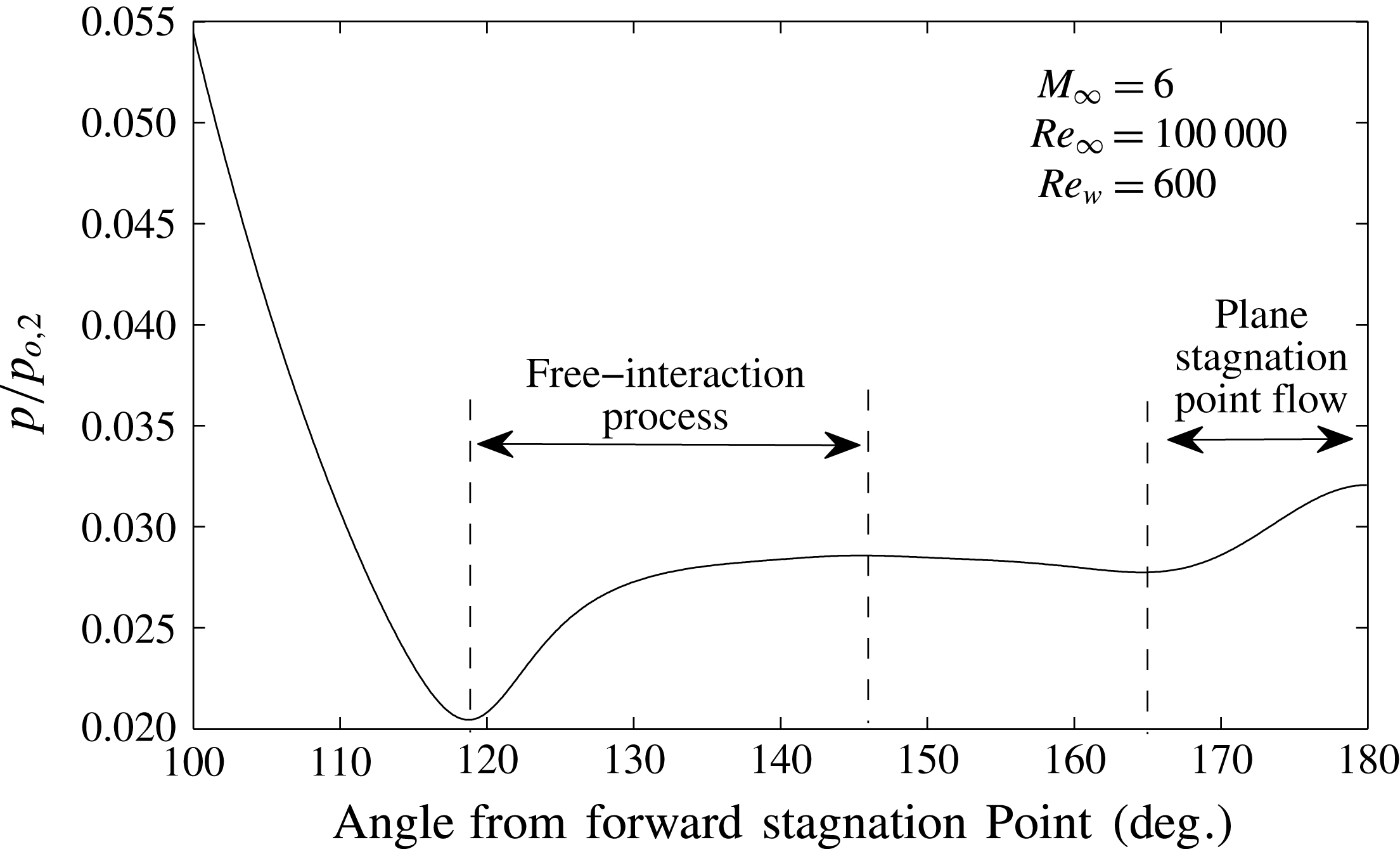
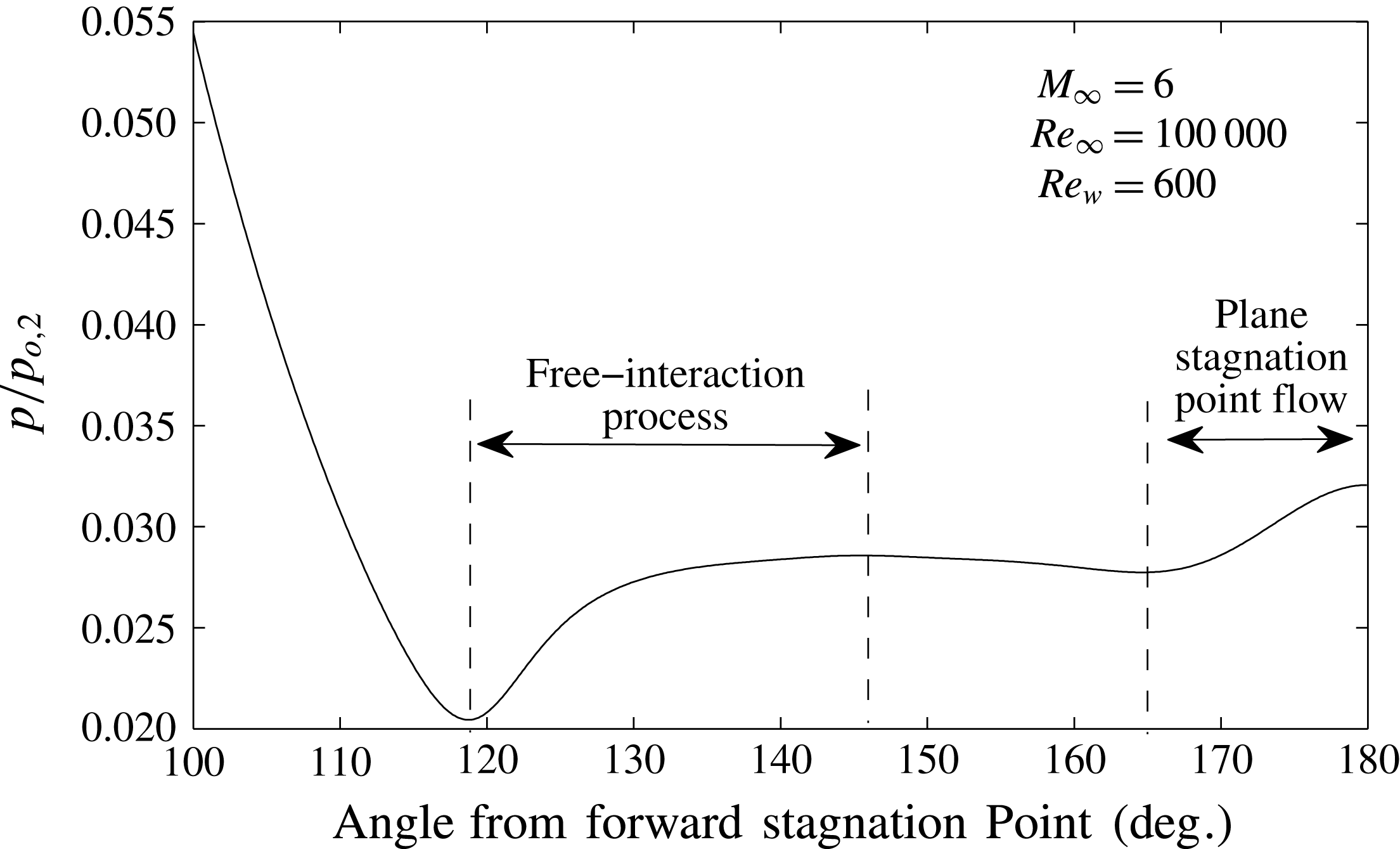
Reference McDaniel, Wright and Songer2011). The simulation result for pressure along the base of an adiabatic circular cylinder at
 $M=6$
and
 $Re=8\times 10^{4}$
is shown in figure 19. The regions of viscous–inviscid interaction are labelled. The separation process begins at approximately
 $118^{\circ }$
in this case. The stagnation point flow occurs between
 $180^{\circ }$
and
 $165^{\circ }$
(approximately 0.26 cylinder radii). Therefore this mechanism occurs over a short distance at the base and will be discussed here as plane stagnation point flow.
Pressure distribution along the cylinder base (Mach 6,
 $Re$
100 000) – planar wake.
Pressure contours in the planar rear-stagnation point region.
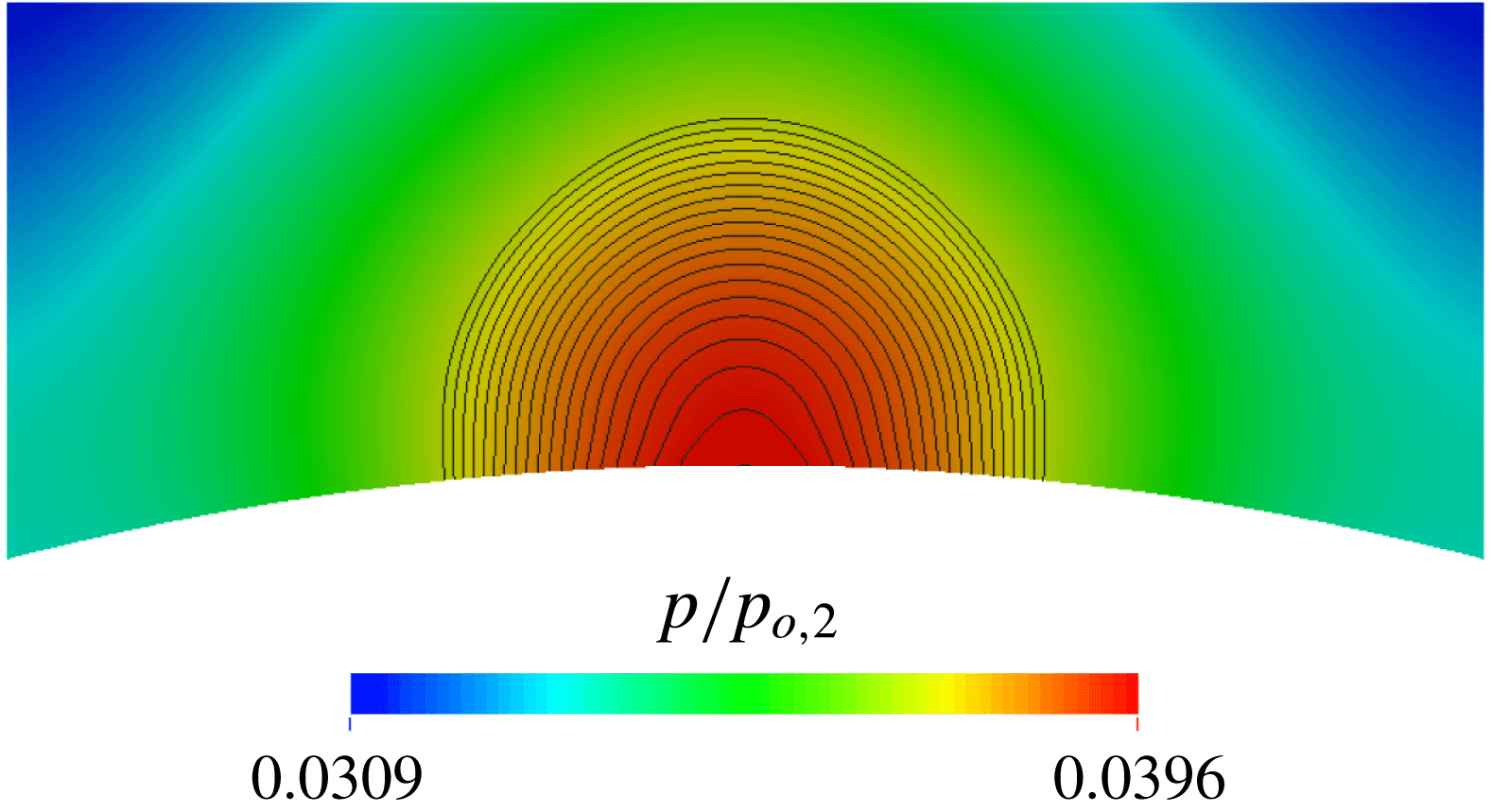
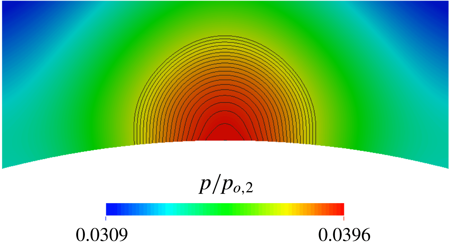
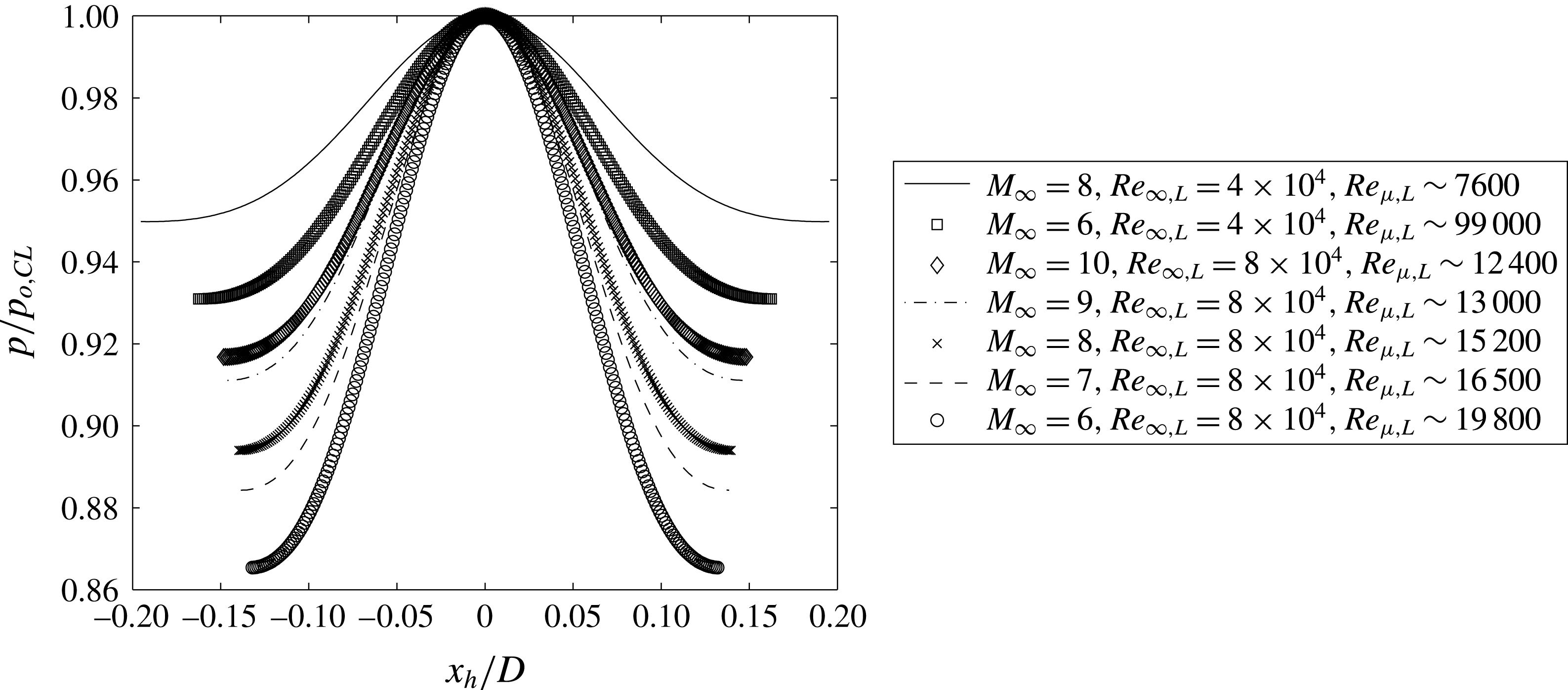
For this analysis, since this mechanism occurs over a short distance and at a relatively low Mach number the flow is analysed as an incompressible stagnation point flow. It is also assumed in the present analysis that the centreline pressure prior to the stagnation interaction is equal to the base pressure after the interaction. This is reinforced by the circular pressure contours visible in figure 20. However, at sufficiently high Reynolds numbers (
 $Re_{\unicode[STIX]{x1D707},L}>2.4\times 10^{4}$
based on the present data), the pressure from the stagnation solution can fall below the pressure coming from the free-interaction process. This is slightly visible in the pressure distribution in figure 19.
Pressure in rear-stagnation point flow (legend in order of increasing
 $Re_{\unicode[STIX]{x1D707}}$
) – planar wake.

To analyse the flow, the pressure distribution in the stagnation region is approximated as the Gaussian (following Tu & Wood (Reference Tu and Wood1996)):
 $$\begin{eqnarray}\displaystyle & \displaystyle p-p_{CL}=\left(p_{o,CL}-p_{CL}\right)\exp \left(\frac{-x_{h}^{2}}{k^{2}}\right), & \displaystyle\end{eqnarray}$$
where
 $x_{h}$
is the distance from the stagnation point along the wall and
 $k$
is a constant. The amplitude of the pressure rise is the difference between the static and stagnation pressure on the centreline (
 $p_{o,CL}-p_{CL}$
). Referring back to figure 10 it can be seen that the stagnation pressure does not change significantly in the direct vicinity of the stagnation interaction. Therefore, using the isentropic definition for the stagnation pressure ratio (4.23) becomes:
 $$\begin{eqnarray}\displaystyle & \displaystyle p-p_{CL}=p_{0,CL}\left[1-\left(1+\frac{\unicode[STIX]{x1D6FE}-1}{2}M_{CL}^{2}\right)^{-\unicode[STIX]{x1D6FE}/(\unicode[STIX]{x1D6FE}-1)}\right]\exp \left(\frac{-x_{h}^{2}}{k^{2}}\right). & \displaystyle\end{eqnarray}$$
Thus by fitting (4.24) to experimental or numerical data, the centreline Mach number
 $M_{CL}$
, and the constant
 $k$
can be found. Additional information can be found from the Gaussian fit through a force analysis. The momentum change required to stagnate the jet coming from the centreline must be equal to the integrated pressure along the wall. Therefore:
 $$\begin{eqnarray}\displaystyle \unicode[STIX]{x1D70C}u_{CL}^{2}\unicode[STIX]{x1D6FF}=p_{CL}\left[\left(1+\frac{\unicode[STIX]{x1D6FE}-1}{2}M_{CL}^{2}\right)^{\unicode[STIX]{x1D6FE}/(\unicode[STIX]{x1D6FE}-1)}-1\right]\int _{-\infty }^{\infty }\exp \left(\frac{-x_{h}^{2}}{k^{2}}\right)\,\text{d}x, & & \displaystyle\end{eqnarray}$$
where
 $\unicode[STIX]{x1D6FF}$
is the effective width of the ‘jet’ coming from the centreline. Noting that the integral of the Gaussian is simply
 $\sqrt{\unicode[STIX]{x03C0}}k$
and that
 $\unicode[STIX]{x1D70C}u_{CL}^{2}=p_{CL}\unicode[STIX]{x1D6FE}M_{CL}^{2}$
this can be rewritten and simplified to:
 $$\begin{eqnarray}\displaystyle k=\frac{\unicode[STIX]{x1D6FF}}{\sqrt{\unicode[STIX]{x03C0}}}\frac{\unicode[STIX]{x1D6FE}M_{CL}^{2}}{\left(1+\displaystyle \frac{\unicode[STIX]{x1D6FE}-1}{2}M_{CL}^{2}\right)^{\unicode[STIX]{x1D6FE}/\unicode[STIX]{x1D6FE}-1}-1}. & & \displaystyle\end{eqnarray}$$
By the same process, in axisymmetric rear-stagnation point flow:
 $$\begin{eqnarray}\displaystyle k=\frac{\unicode[STIX]{x1D6FF}}{2}\left[\frac{\unicode[STIX]{x1D6FE}M_{CL}^{2}}{\left(1+\displaystyle \frac{\unicode[STIX]{x1D6FE}-1}{2}M_{CL}^{2}\right)^{\unicode[STIX]{x1D6FE}/\unicode[STIX]{x1D6FE}-1}-1}\right]^{1/2}. & & \displaystyle\end{eqnarray}$$
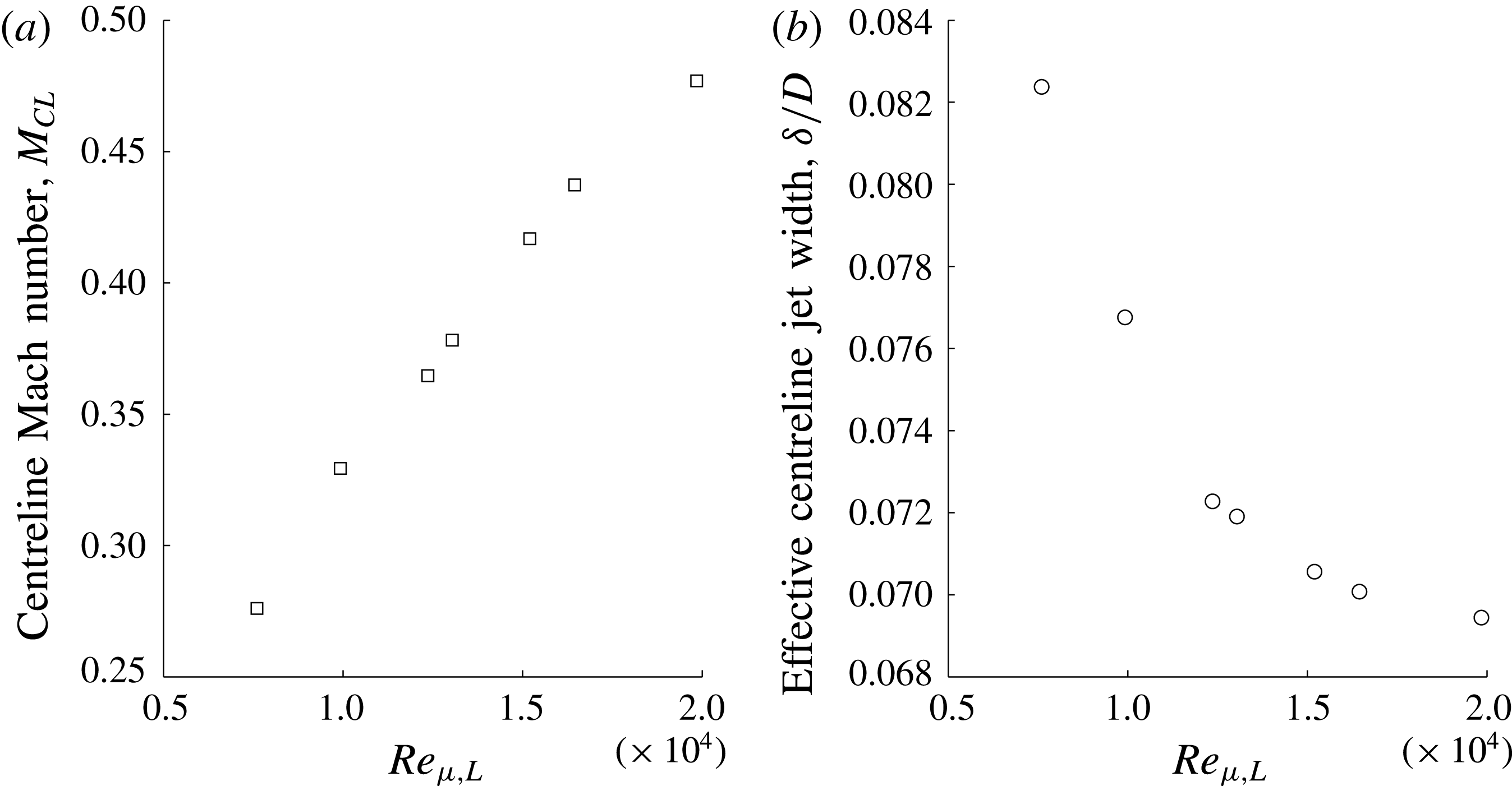
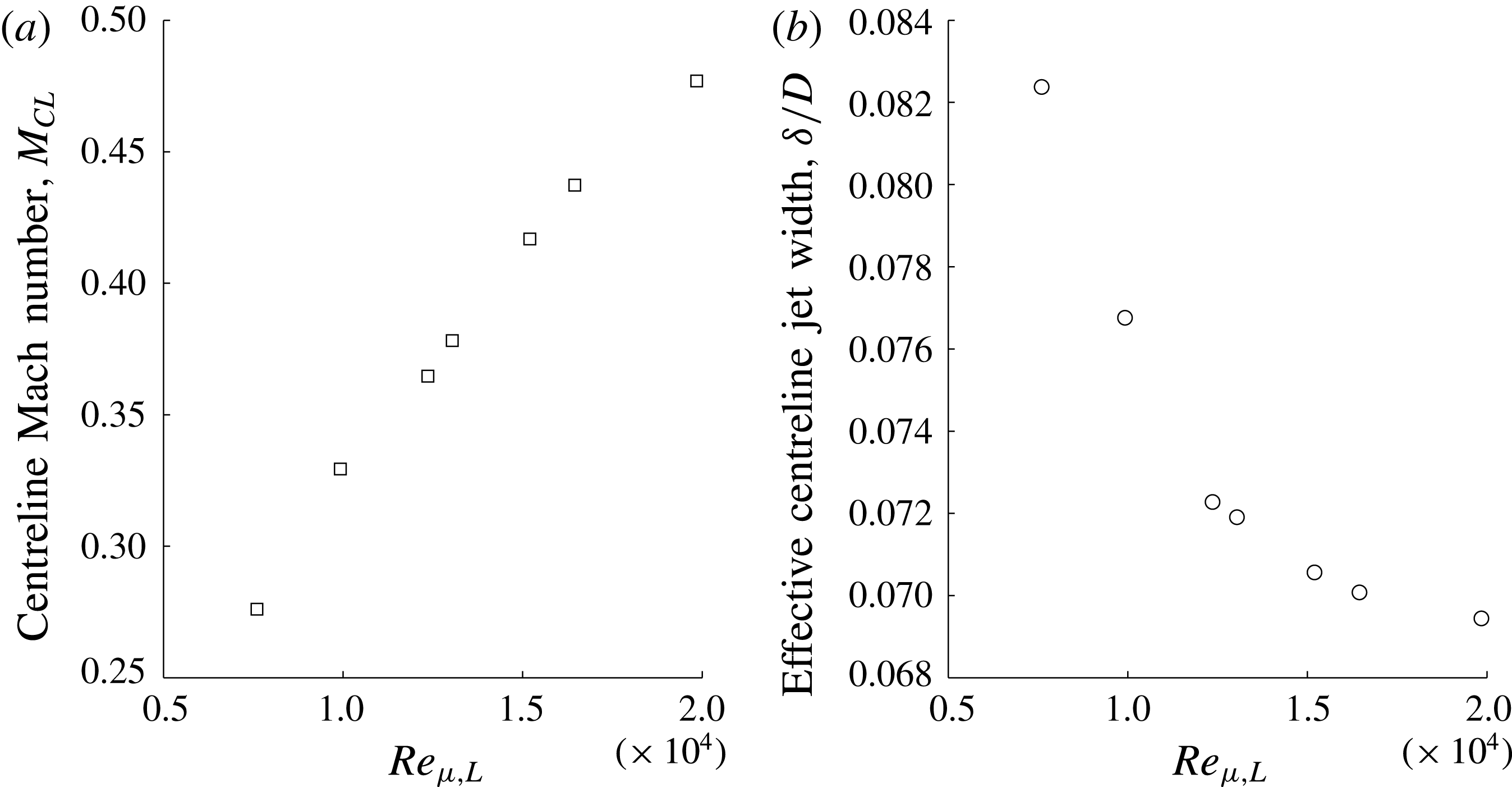
A small stagnation pressure increase is observed in figure 21, the pressure distributions in the rear stagnation region are plot at a range of Reynolds and Mach numbers. From the figure, the post-shock Reynolds number appears to be the major driver. These distributions were fit using the exponential function in (4.24). With these fits it is possible to estimate the centreline Mach number, and the effective jet diameter of the centreline flow. These are plotted in figure 22. As post-shock Reynolds number is increased, the centreline Mach number increases and the effective jet diameter decreases. These observations are consistent with the increasing convective nature as the wake Reynolds number is increased. As the constant vorticity core grows, this effectively decreases the width of the centreline jet. As well, as the diffusion is decreased the flow in the wake is faster, increasing the centreline Mach number. The same process could be used for an experimental base pressure distribution to estimate centreline Mach number and effective jet width.
Centreline Mach number predicted from base pressure distribution – planar wake.
4.5 Viscous reattachment flow
In order to understand how the wake recirculation feedback mechanism fits into the overall wake mechanism the reattachment process must be discussed. It is known that reattachment can be adequately modelled by integral momentum viscous–inviscid interaction methods such as those of Crocco & Lees (Reference Crocco and Lees1952) and Reeves & Lees (Reference Reeves and Lees1965). It is also known that free interaction can be used to describe reattachment in boundary layers (Settles & Williams Reference Settles and Williams1982; Delery Reference Delery, Babinsky and Harvey2011). However, wake reattachment requires special treatment for free-interaction theory. Here, a free-interaction theory is presented based on the integral momentum form of the boundary layer equations. The interaction model employed here differs by the equations used in its formulation, as well as the wake specific scaling properties employed. In the present derivation it is assumed that the appropriate scaling properties for the entire wake are the properties at the lip separation shock interaction onset. Therefore, pressure, shear stress, streamwise and stream normal lengths are non-dimensionalized by
 $q_{e,0}$
,
 $\unicode[STIX]{x1D70F}_{0}$
,
 $L_{sep}$
, and
 $\unicode[STIX]{x1D6FF}_{0}^{\ast }$
, respectively.
4.5.1 Planar wake reattachment
Beginning with the integral momentum equation:
 $$\begin{eqnarray}\displaystyle & \displaystyle \frac{\text{d}}{\text{d}x}\left(\unicode[STIX]{x1D70C}_{e}u_{e}^{2}\unicode[STIX]{x1D703}\right)+\unicode[STIX]{x1D70C}_{e}u_{e}\frac{\text{d}u_{e}}{\text{d}x}\unicode[STIX]{x1D6FF}^{\ast }=0. & \displaystyle\end{eqnarray}$$
The integral momentum equation is preferred due to the absence of shear stress at the centreline. This equation can be integrated through reattachment by including continuity and mechanical energy equations, and a family of velocity profiles (as was done by Reeves & Lees (Reference Reeves and Lees1965) and Grange et al. (Reference Grange, Klineberg and Lees1967)). However, this is not the focus of the present work. By including (from the streamwise Euler equation)
 $\text{d}u_{e}=-\text{d}p_{e}/\unicode[STIX]{x1D70C}_{e}u_{e}$
, and assuming that
 $\text{d}\unicode[STIX]{x1D70C}_{e}U_{e}/\text{d}x$
is negligible, the integral momentum equation can be rearranged to give:
 $$\begin{eqnarray}\displaystyle & \displaystyle \frac{1}{q_{e}}\frac{\text{d}p}{\text{d}x}=\frac{2}{H^{-1}+1}\frac{1}{\unicode[STIX]{x1D6FF}^{\ast }}\frac{\text{d}\unicode[STIX]{x1D703}}{\text{d}x}, & \displaystyle\end{eqnarray}$$
where
 $q_{e}$
is the dynamic pressure, and
 $H$
is the viscous layer shape factor. Utilizing a linearized compression along the external streamline, borrowing from the process of modified free interaction from Hinman & Johansen (Reference Hinman and Johansen2016a
) the external flow can be modelled with:
 $$\begin{eqnarray}\displaystyle & \displaystyle \frac{\sqrt{M_{e}^{2}-1}}{2q_{e}}\frac{\text{d}p}{\text{d}x}=\frac{\text{d}\unicode[STIX]{x1D6FF}^{\ast }}{\text{d}x}+\unicode[STIX]{x0394}\unicode[STIX]{x1D713}, & \displaystyle\end{eqnarray}$$
where
 $\text{d}\unicode[STIX]{x1D6FF}^{\ast }/\text{d}x$
and
 $\unicode[STIX]{x0394}\unicode[STIX]{x1D713}$
are the viscous layer displacement effect and the inviscid turning angle (wake angle), respectively. To formulate a free-interaction theory, these terms must be normalized. It is not obvious how the wake turning angle should be scaled. First, using the small angle approximation, it can be assumed that:
 $$\begin{eqnarray}\displaystyle & \displaystyle \unicode[STIX]{x0394}\unicode[STIX]{x1D713}\approx \frac{h}{L_{w}}. & \displaystyle\end{eqnarray}$$
From the control volume analysis (while still assuming a triangular wake), it can be shown that:
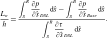 $$\begin{eqnarray}\displaystyle & \displaystyle \frac{L_{w}}{h}=\frac{\displaystyle \int _{S}^{R}\frac{\unicode[STIX]{x2202}p}{\unicode[STIX]{x2202}{\hat{s}}}_{DSL}\,\text{d}{\hat{s}}-\int _{S}^{B}\frac{\unicode[STIX]{x2202}p}{\unicode[STIX]{x2202}{\hat{s}}}_{Base}\,\text{d}{\hat{s}}}{\displaystyle \int _{S}^{R}\frac{\unicode[STIX]{x2202}\unicode[STIX]{x1D70F}}{\unicode[STIX]{x2202}{\hat{s}}}_{DSL}\,\text{d}{\hat{s}}}. & \displaystyle\end{eqnarray}$$
Since the pressure is continuous around the boundaries of the wake:
 $$\begin{eqnarray}\displaystyle & \displaystyle \frac{L_{w}}{h}=\frac{\displaystyle \int _{B}^{R}\frac{\unicode[STIX]{x2202}p}{\unicode[STIX]{x2202}{\hat{s}}}_{CL}\,\text{d}{\hat{s}}}{\displaystyle \int _{S}^{R}\frac{\unicode[STIX]{x2202}\unicode[STIX]{x1D70F}}{\unicode[STIX]{x2202}{\hat{s}}}_{DSL}\,\text{d}{\hat{s}}}. & \displaystyle\end{eqnarray}$$
From the momentum equation analysis, it was shown that:
 $$\begin{eqnarray}\displaystyle & \displaystyle \int _{B}^{R}\frac{\unicode[STIX]{x2202}p}{\unicode[STIX]{x2202}{\hat{s}}}\,\text{d}{\hat{s}}=-\int _{B}^{R}\frac{\unicode[STIX]{x2202}\unicode[STIX]{x1D714}_{\hat{z}}}{\unicode[STIX]{x2202}\hat{n}}\,\text{d}{\hat{s}}-\int _{B}^{R}\unicode[STIX]{x1D70C}u\frac{\unicode[STIX]{x2202}u}{\unicode[STIX]{x2202}{\hat{s}}}\,\text{d}{\hat{s}}. & \displaystyle\end{eqnarray}$$
Combining and normalizing:
 $$\begin{eqnarray}\displaystyle & \displaystyle \frac{L_{w}}{h}=\frac{-\unicode[STIX]{x1D707}_{0}\unicode[STIX]{x1D714}_{z,0}\displaystyle \frac{L_{sep}}{\unicode[STIX]{x1D6FF}_{0}^{\ast }}\int _{B}^{R}\unicode[STIX]{x1D707}^{\prime }\frac{\unicode[STIX]{x2202}\unicode[STIX]{x1D714}_{\hat{z}}^{\prime }}{\unicode[STIX]{x2202}\hat{n}^{\prime }}\,\text{d}{\hat{s}}^{\prime }-2q_{e,0}\int _{B}^{R}\unicode[STIX]{x1D70C}^{\prime }u^{\prime }\frac{\unicode[STIX]{x2202}u^{\prime }}{\unicode[STIX]{x2202}\hat{s^{\prime }}}\,\text{d}{\hat{s}}^{\prime }}{\unicode[STIX]{x1D70F}_{0}\unicode[STIX]{x1D70F}_{DSL}^{\prime }}. & \displaystyle\end{eqnarray}$$
Therefore the dimensions of the wake recirculation region must follow some function of the form:
 $$\begin{eqnarray}\displaystyle \frac{L_{w}}{h}=\frac{L_{sep}}{\unicode[STIX]{x1D6FF}_{0}^{\ast }}C_{1}+\frac{2}{C_{f,0}}C_{2}. & & \displaystyle\end{eqnarray}$$
 $C_{1}$
and
 $C_{2}$
are dimensionless functions that represent the ratio of viscous vorticity flux and non-conservative advection to the dividing streamline shear stress, respectively. Using the boundary layer equations at the wall in the separation interaction region, the gross approximation can be made that
 $C_{f,0}\sim \unicode[STIX]{x1D6FF}_{0}^{\ast }/L_{sep}$
. This leads to the fact that:
 $$\begin{eqnarray}\displaystyle & \displaystyle \frac{L_{w}}{h}\sim \frac{L_{sep}}{\unicode[STIX]{x1D6FF}_{0}^{\ast }}. & \displaystyle\end{eqnarray}$$
However, this does not account for the full mechanism of the lip-shock interaction. From free-interaction theory, it is known that
 $L_{sep}/\unicode[STIX]{x1D6FF}_{0}^{\ast }\sim C_{f,0}^{-1/2}\left(M_{0}^{2}-1\right)^{-1/4}$
(Delery Reference Delery, Babinsky and Harvey2011; Hinman & Johansen Reference Hinman and Johansen2016a
). This would lead to a more accurate expression of the wake size:
 $$\begin{eqnarray}\displaystyle & \displaystyle \frac{L_{w}}{h}=\frac{L_{sep}}{\unicode[STIX]{x1D6FF}_{0}^{\ast }}C_{1}+\sqrt{M_{0}^{2}-1}\left(\frac{L_{sep}}{\unicode[STIX]{x1D6FF}_{0}^{\ast }}\right)^{2}C_{3}, & \displaystyle\end{eqnarray}$$
where
 $C_{1}$
and
 $C_{3}$
are dimensionless functions that could be determined empirically. This is an example of how the sub-mechanisms within the present theoretical framework can be further analysed in future works. However, for simplicity in the rest of the present section, it will be assumed that
 $\unicode[STIX]{x0394}\unicode[STIX]{x1D713}\approx h/L_{w}\sim \unicode[STIX]{x1D6FF}_{0}^{\ast }/L_{sep}$
.
With the new scaling of the wake angle, equations (4.29) and (4.30) can be normalized based on properties upstream of the wake, linearized and integrated from the reattachment point to the neck. By taking the product of these equations the resulting free-interaction equation is:
 $$\begin{eqnarray}\displaystyle & \displaystyle \frac{p_{N}-p_{R}}{q_{e,0}}=\frac{2C_{f,0}^{1/2}}{\left(M_{0}^{2}-1\right)^{1/4}\left(H_{0}^{-1}+1\right)^{1/2}}F_{r,N}. & \displaystyle\end{eqnarray}$$
Here,
 $F_{r,N}$
is the viscous reattachment interaction parameter and is a correlation parameter between the pressure rise between the reattachment and the neck (
 $p_{N}-p_{R}$
) versus the properties upstream of the wake.
 $F_{r,N}$
is plotted in figure 23. If perfect similarity was observed,
 $F_{r,N}$
would be constant for all cases. From figure 23, as Reynolds number increases
 $F_{r,N}$
approaches increasingly similar behaviour. The neck pressure is assumed to be dictated by the reattachment shock angle, and is the pressure rise resulting from the flow being redirected to the flow centreline. From (4.39) it can be shown that the difference between the neck pressure and the reattachment pressure scales such that:
 $$\begin{eqnarray}\displaystyle & \displaystyle \frac{p_{R}}{q_{0}}=\frac{p_{N}}{q_{0}}-O\left[Re^{-1/4}(M_{0}^{2}-1)^{-1/4}\left(H_{0}^{-1}+1\right)^{-1/2}\right]. & \displaystyle\end{eqnarray}$$
For a single geometry, due to hypersonic similarity, this can be further simplified to:
 $$\begin{eqnarray}\displaystyle & \displaystyle \frac{p_{R}}{q_{0}}=\frac{p_{N}}{q_{0}}-O\left[Re^{-1/4}\right]. & \displaystyle\end{eqnarray}$$
Additionally, as the parameter
 $F_{r,N}$
is observed to be mostly Reynolds number independent (for
 $Re_{\unicode[STIX]{x1D707},L}>5000$
), the scaling argument that
 $h/L_{w}\sim \unicode[STIX]{x1D6FF}_{0}/L_{sep}$
is reasonable. Further, this indicates that the wake dimensions should scale such that
 $h/L_{w}\sim C_{f,0}^{1/2}\left(M_{0}^{2}-1\right)^{1/2}$
.
Reattachment parameter
 $F_{r,N}$
as a function of post-shock Reynolds number.
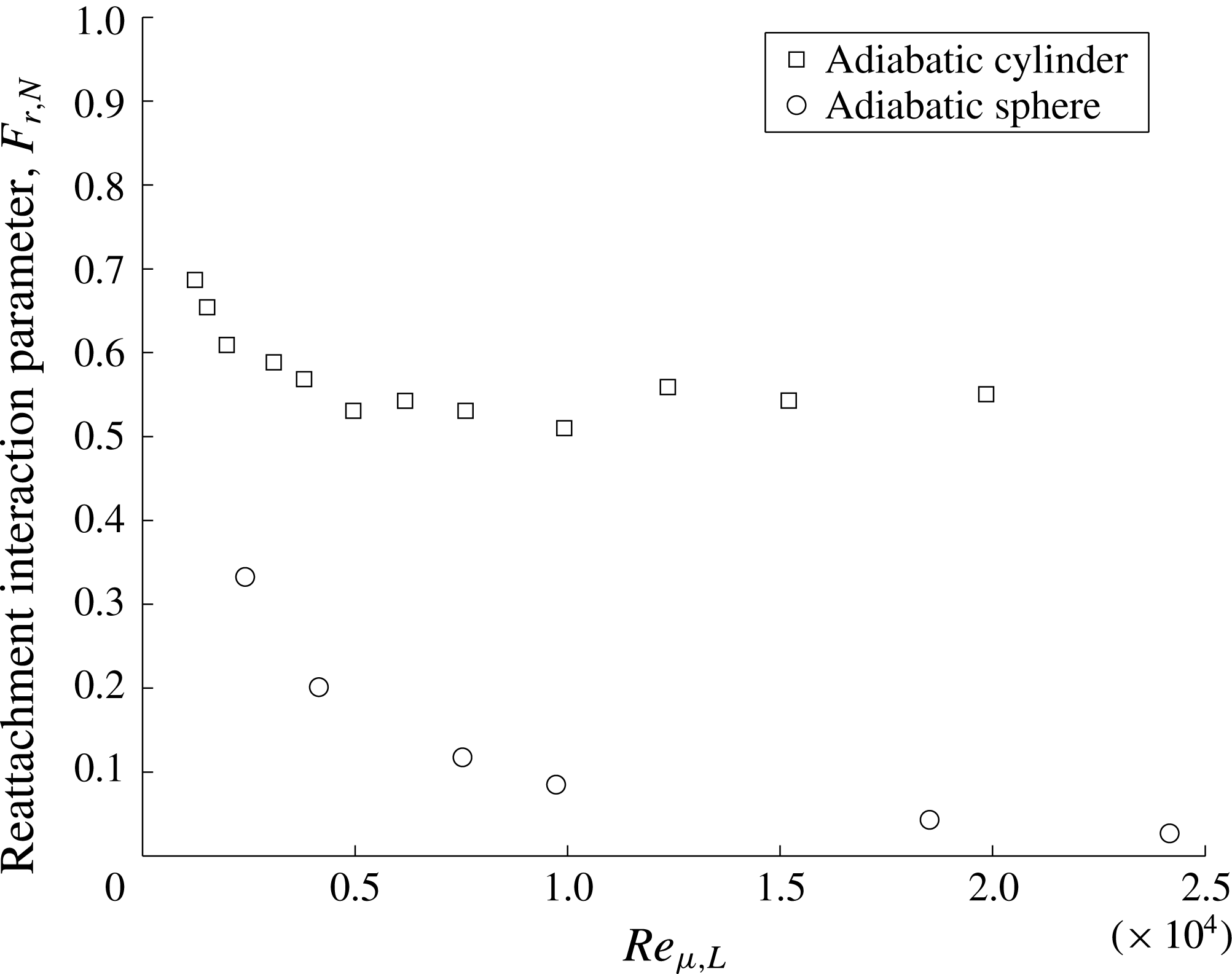
4.5.2 Axisymmetric wake reattachment
In axisymmetric flow, the formulation is similar, however the momentum integral equation is written as:
 $$\begin{eqnarray}\displaystyle & \displaystyle \frac{\text{d}}{\text{d}x}\left(\unicode[STIX]{x1D70C}_{e}u_{e}\unicode[STIX]{x1D703}^{2}\right)+\unicode[STIX]{x1D70C}_{e}u_{e}\frac{\text{d}u_{e}}{\text{d}x}\unicode[STIX]{x1D6FF}^{\ast 2}=0, & \displaystyle\end{eqnarray}$$
where the displacement and momentum thicknesses in the wake are:
 $$\begin{eqnarray}\displaystyle & \displaystyle \unicode[STIX]{x1D6FF}^{\ast }=\left(\frac{1}{\unicode[STIX]{x03C0}}\int _{0}^{\unicode[STIX]{x1D6FF}}\left(1-\frac{\unicode[STIX]{x1D70C}u}{\unicode[STIX]{x1D70C}_{e}u_{e}}\right)r\,\text{d}r\right)^{0.5}, & \displaystyle\end{eqnarray}$$
 $$\begin{eqnarray}\displaystyle & \displaystyle \unicode[STIX]{x1D703}=\left(\frac{1}{\unicode[STIX]{x03C0}}\int _{0}^{\unicode[STIX]{x1D6FF}}\frac{\unicode[STIX]{x1D70C}u}{\unicode[STIX]{x1D70C}_{e}u_{e}}\left(1-\frac{u}{u_{e}}\right)r\,\text{d}r\right)^{0.5}. & \displaystyle\end{eqnarray}$$
In axisymmetric flow at the wall (at separation) the definition of displacement and momentum thickness from Hrubecky (Reference Hrubecky1963) should be used. After applying the same assumptions and process as performed in planar flow, the equation for the reattachment interaction becomes:
 $$\begin{eqnarray}\displaystyle & \displaystyle \frac{p_{R}}{q_{0}}=\frac{p_{N}}{q_{0}}-\frac{\sqrt{8}C_{f,0}^{1/2}}{\left(M_{0}^{2}-1\right)^{1/4}\left(H_{0}^{-1}+H_{0}\right)^{1/2}}F_{r,N}. & \displaystyle\end{eqnarray}$$
The reattachment interaction parameter
 $F_{r,N}$
based on (4.45) is plotted in figure 23. The results show that in the axisymmetric case, the parameter
 $F_{r,N}$
is more Reynolds number dependent than in the planar case. This is due to the fact that the planar linear compression (4.30) is used. This leads to an additional Reynolds number dependence that is visible in the results. Additional work is warranted to find a Reynolds number-independent version of the reattachment interaction for axisymmetric wakes.
5 Summary of the overall wake mechanism
5.1 Mechanistic summary
Since the recirculation region forms a set of well-defined boundaries between the rear-stagnation point, the reattachment point and the separation point, the overall near-wake mechanism can be described by combining the mechanisms along each section. The mechanistic sections are illustrated in figure 24, and each sub-mechanism is summarized here. (i) First, the boundary layer on the body approaching the wake separates and forms the lip separation shock. This process can be accurately described by free-interaction theory as was shown by Hinman & Johansen (Reference Hinman and Johansen2016a ,Reference Hinman and Johansen c ). (ii) Between the separation point and the wake reattachment point, momentum and energy are transferred between the inner and outer wake by processes dominated by diffusion. Pressure is gained along this streamline by diffusion of vorticity normal to the streamline and by non-conservative advection. The process along this streamline leads to a decrease in entropy along the streamline length due to heat diffusion away from the streamline. (iii) The pressure at the reattachment point is dictated by a balance between the maximum pressure that can be gained by the dividing streamline through sub-mechanism (ii), and the pressure rise impressed by the reattachment shock wave. The recompression mechanism is a viscous–inviscid interaction that was explained in § 4.5 utilizing an integral formulation of the momentum equation. (iv) Along the centreline, stagnation pressure is lost due to diffusion of vorticity along the centreline and non-conservative advection. In contrast to the dividing streamline, the centreline becomes less dominated by viscous vorticity flux as Reynolds number is increased. At high Reynolds number the contribution from the non-conservative advection of momentum becomes an important means of stagnation pressure loss along the centreline. (v) As the flow approaches the base, a viscous planar stagnation point flow occurs. It was shown that the magnitude of the pressure change in this interaction is primarily a function of centreline Mach number, which in turn is a function of post-shock or wake Reynolds number. The closed loop created by sub-mechanisms (i), (ii), (iv) and (v) is referred to as the recirculation feedback mechanism as it links the separation (i) and reattachment (iii) mechanisms.
Illustration of overall near-wake mechanism.
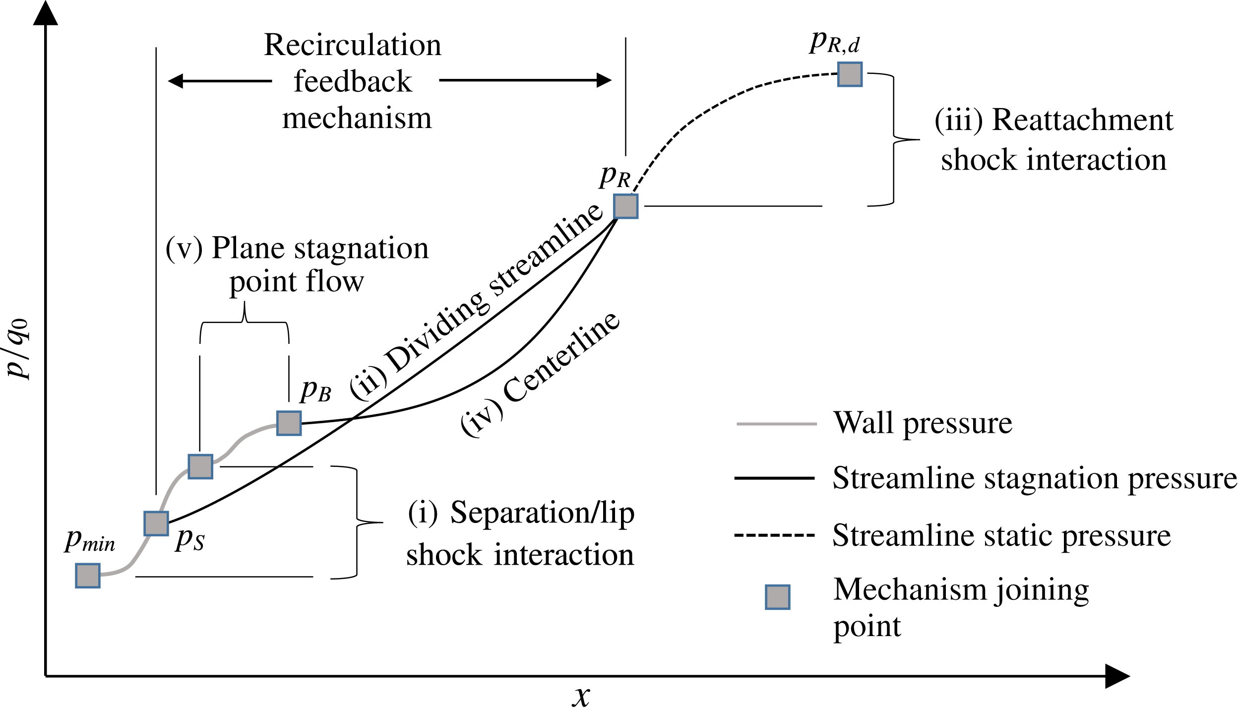
The recirculation feedback mechanism can now be demonstrated by linking each of the equations described in the previous sections in terms of pressure. While pressure is chosen here, alternative sets of equations could be derived since all parameters must be continuous around the closed streamlines. Energy, entropy and vorticity are examples of properties that must be continuous when the streamline is closed.
Free interaction as derived by Hinman & Johansen (Reference Hinman and Johansen2016c ) for curved surfaces is:
 $$\begin{eqnarray}\displaystyle & \displaystyle \frac{\unicode[STIX]{x0394}p}{q_{o}}=F^{\ast }\sqrt{\frac{2C_{fo}}{\left(M_{o}^{2}-1\right)^{1/2}}}. & \displaystyle\end{eqnarray}$$
In this equation
 $F^{\ast }$
is a correlation parameter between the properties at the interaction onset (
 $C_{fo}$
,
 $M_{e,o}$
,
 $q_{e,o}$
) and the pressure rise due to the separation shock (
 $\unicode[STIX]{x0394}p$
). Since this theory is based on the boundary layer approximation, the pressure change is also equivalent to the change in stagnation pressure at the wall: (
 $\unicode[STIX]{x0394}p_{o}$
). Taking the difference between (5.1) at separation and after the lip-shock formation yields:
 $$\begin{eqnarray}\displaystyle & \displaystyle \frac{\unicode[STIX]{x0394}p_{sep,int}}{q_{o}}=\unicode[STIX]{x0394}F^{\ast }\sqrt{\frac{2C_{fo}}{\left(M_{o}^{2}-1\right)^{1/2}}}. & \displaystyle\end{eqnarray}$$
Here,
 $\unicode[STIX]{x0394}F^{\ast }$
is the difference between the value of
 $F^{\ast }$
at separation, and at the plateau value.
The magnitude of the pressure rise in the viscous planar stagnation point flow is given by
 $p_{o,CL}-p_{CL}$
. This can be rewritten in terms of centreline stagnation pressure and Mach number:
 $$\begin{eqnarray}\displaystyle & \displaystyle \unicode[STIX]{x0394}p_{RSP}=p_{o,CL}\left[1-\left(1-\frac{\unicode[STIX]{x1D6FE}-1}{2}M_{CL}^{2}\right)^{-\unicode[STIX]{x1D6FE}/(\unicode[STIX]{x1D6FE}-1)}\right]. & \displaystyle\end{eqnarray}$$
Therefore the total pressure rise between separation and the rear-stagnation point is:
 $$\begin{eqnarray}\displaystyle & \displaystyle \unicode[STIX]{x0394}p_{S,B}=q_{o}\unicode[STIX]{x0394}F^{\ast }\sqrt{\frac{2C_{fo}}{\left(M_{o}^{2}-1\right)}}+p_{0,CL}\left[1-\left(1+\frac{\unicode[STIX]{x1D6FE}-1}{2}M_{CL}^{2}\right)^{-\unicode[STIX]{x1D6FE}/(\unicode[STIX]{x1D6FE}-1)}\right]. & \displaystyle\end{eqnarray}$$
From § 4.3, the relation for the stagnation pressure rise around the streamlines in the wake is repeated here:
 $$\begin{eqnarray}\displaystyle & \displaystyle \unicode[STIX]{x0394}p_{S,B}=p_{o,B}-p_{o,S}=-\int _{S}^{B}\unicode[STIX]{x1D707}\frac{\unicode[STIX]{x2202}\unicode[STIX]{x1D714}_{z}}{\unicode[STIX]{x2202}\hat{n}}\,\text{d}{\hat{s}}-\int _{S}^{B}\unicode[STIX]{x1D70C}u_{{\hat{s}}}\frac{\unicode[STIX]{x2202}u_{{\hat{s}}}}{\unicode[STIX]{x2202}s}\,\text{d}s. & \displaystyle\end{eqnarray}$$
Since the changes in pressure around the boundaries must be equal, equations (5.4) and (5.5) must balance. It is useful to normalize (5.4) and (5.5) by the dynamic pressure upstream of the lip-shock interaction. Additionally, in (5.5), the centreline and dividing streamline sections should be separated and the remaining dimensional variables should be normalized in a fashion consistent with free-interaction theory. This process yields:
 $$\begin{eqnarray}\displaystyle & & \displaystyle \underbrace{\unicode[STIX]{x0394}F^{\ast }\sqrt{\frac{2C_{fo}}{\left(M_{o}^{2}-1\right)^{1/2}}}}_{\text{Lip Shock Interaction}}+\underbrace{\frac{p_{0,CL}}{q_{0}}\left[1-\left(1+\frac{\unicode[STIX]{x1D6FE}-1}{2}M_{CL}^{2}\right)^{-\unicode[STIX]{x1D6FE}/(\unicode[STIX]{x1D6FE}-1)}\right]}_{\text{Plane}\,\,\text{Stagnation}\,\,\text{Point}\,\,\text{Interaction}}\nonumber\\ \displaystyle & & \displaystyle \quad =-\,\underbrace{\frac{\unicode[STIX]{x1D707}_{0}\unicode[STIX]{x1D714}_{0}}{q_{0}}\frac{L_{sep}}{\unicode[STIX]{x1D6FF}_{0}}\left[W_{DSL}+W_{CL}\right]}_{\text{Viscous Vorticity Flux}}-\underbrace{\left[A_{DSL}+A_{CL}\right]}_{\text{Non-conservative Advection}}.\end{eqnarray}$$
The
 $W$
and
 $A$
terms represent the normalized integrals of viscous vorticity flux and advection, respectively. Equation (5.6) is a non-dimensional representation of the near-wake streamline momentum transfer balance. The mechanism in (5.6) describes the feedback between separation and reattachment shocks. It is useful to examine how reattachment pressure fits into the overall wake mechanism. As well, due to the limitations of assumptions used to formulate
 $W_{CL}$
(see § 4), it is advantageous to not address this term explicitly. By including the pressure decrease along the centreline explicitly, the mechanism can be written as:
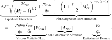 $$\begin{eqnarray}\displaystyle & & \displaystyle \underbrace{\unicode[STIX]{x0394}F^{\ast }\sqrt{\frac{2C_{fo}}{\left(M_{o}^{2}-1\right)^{1/2}}}}_{\text{Lip Shock Interaction}}+\underbrace{\frac{p_{0,CL}}{q_{0}}\left[-\left(1+\frac{\unicode[STIX]{x1D6FE}-1}{2}M_{CL}^{2}\right)^{-\unicode[STIX]{x1D6FE}/(\unicode[STIX]{x1D6FE}-1)}\right]}_{\text{Plane Stagnation Point Interaction}}\nonumber\\ \displaystyle & & \displaystyle \quad =-\,\underbrace{\frac{\unicode[STIX]{x1D707}_{0}\unicode[STIX]{x1D714}_{0}}{q_{0}}\frac{L_{sep}}{\unicode[STIX]{x1D6FF}_{0}}\left[W_{DSL}\right]}_{\text{Viscous Vorticity FLux}}\underbrace{-\left[A_{DSL}\right]}_{\text{Non-Conservative Advection}}\underbrace{-\frac{p_{R}}{q_{o}}}_{\text{Reattachment Pressure}}.\end{eqnarray}$$
Equation (5.7) and the reattachment process ((4.40) or (4.45) for planar or axisymmetric flow, respectively) must be consistent with each other. These three equations constitute the first overall theoretical framework of the laminar near-wake mechanism including separation, reattachment, rear-stagnation point flow and dividing streamline stagnation pressure gain for both planar and axisymmetric near wakes.
By examining each term, the effect of upstream properties, Reynolds number and Mach number can be discussed. Firstly, it is important to notice that free-stream Mach number does not appear explicitly anywhere in the balance. The primary effect of free-stream Mach number is to alter the post-shock properties. The first term on the left-hand side is the free-interaction formulation from Hinman & Johansen (Reference Hinman and Johansen2016a
). Due to hypersonic similarity (when
 $M>5$
),
 $M_{o}$
is mostly fixed. Therefore the primary coefficient is
 $\sqrt{C_{fo}}$
, which is a function of post-shock Reynolds number. Thus this term is of order
 $Re_{\unicode[STIX]{x1D707}}^{-1/4}$
. The second term on the right-hand side is more complicated to discuss. The function
 $[-\left(1+(\unicode[STIX]{x1D6FE}-1)/2\,M_{CL}^{2}\right)^{-\unicode[STIX]{x1D6FE}/\unicode[STIX]{x1D6FE}-1}]$
can only vary between 0 and 1, while the term
 $p_{o,CL}/q_{o}$
is the ratio between the total pressure along the wake centreline and the dynamic pressure at the separation interaction onset. Both of these components of the term are Reynolds number dependent but the overall term should be of order of magnitude 1. The first term on the right-hand side represents the stagnation pressure gained along the length of the dividing streamline. The coefficient is
 $(\unicode[STIX]{x1D707}_{0}\unicode[STIX]{x1D714}_{0}/q_{0})\,(L_{sep}/\unicode[STIX]{x1D6FF}_{0})$
. By noting that
 $\unicode[STIX]{x1D707}_{0}\unicode[STIX]{x1D714}_{0}/q_{0}=C_{f,0}$
, and that from free-interaction theory
 $L_{sep}/\unicode[STIX]{x1D6FF}_{0}^{\ast }\sim C_{f,0}^{-1/2}\left(M_{0}^{2}-1\right)^{-1/4}$
it can be shown that the coefficient of this term scales with
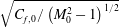 $\sqrt{C_{f,0}/\left(M_{0}^{2}-1\right)^{1/2}}$
. Thus, the viscous terms on the left- and right-hand side of (5.6) scale together (both with
 $Re_{\unicode[STIX]{x1D707}}^{-1/4}$
). The terms
 $A_{DSL}$
and
 $A_{CL}$
represent any non-conservative advection along the wake streamlines. Recall that non-conservative advection results from the non-constant density in the advective terms. Normalized by the dynamic pressure at the interaction onset, these terms are of the order of magnitude of 1. All of the normalized terms,
 $W$
,
 $A$
,
 $M_{CL}$
,
 $p_{0,CL}/q_{0}$
and
 $\unicode[STIX]{x0394}F^{\ast }$
are still Reynolds number dependent and could be analysed in more detail. For example, it was shown that the free-interaction lip-shock formation could be further decomposed into contributions from boundary layer growth and angle change due to the shoulder expansion (Hinman & Johansen Reference Hinman and Johansen2016a
).
It was previously shown using control volume analysis and pertinent wake mechanisms that the wake size (specifically the recirculation region) should scale such that
 $h/L_{w}\sim C_{f,0}^{1/2}\left(M_{0}^{2}-1\right)^{1/2}$
. This can also be explained physically using the present theoretical framework. A graphically representation is shown in figure 25. As wake length
 $L_{w}$
increases, the turning angle at recompression decreases (therefore
 $p_{N}$
decreases). Additionally, as Reynolds number decreases, the fraction of this pressure reached at reattachment gets smaller. These effects are shown by the multiple dashed lines. The solid lines represent the pressure rise dictated by the recirculation feedback mechanism. At lower Reynolds numbers, diffusion of vorticity across the streamline is increased and therefore stagnation pressure is gained faster. Where the lines intersect (and therefore these two effects are balanced) dictates the wake length and the wake reattachment and base pressure.
Illustration of balance between recirculation feedback mechanism and viscous reattachment mechanism.

The overall wake mechanism summary has demonstrated that the defining parameters of the near wake are the Mach number (
 $M_{0}$
) and coefficient of friction (
 $C_{f,0}$
) at the shoulder (or at the separation interaction onset/pressure minimum), the post-shock Reynolds number (
 $Re_{\unicode[STIX]{x1D707}}$
) and the wake Reynolds number (
 $Re_{w,h}$
). Based on this, recommendations for how to explain and discuss experimental and numerical observations are given here. For a single geometry, due to hypersonic similarity,
 $C_{f,0}$
and
 $M_{0}$
will be primarily dependent on post-shock Reynolds number,
 $Re_{\unicode[STIX]{x1D707}}$
. Therefore post-shock Reynolds number is the fundamental parameter of interest. When comparing different geometries however,
 $C_{f,0}$
and
 $M_{0}$
will be geometry dependent.
 $C_{f,0}$
is a function of the vorticity generated upstream that can then be diffused into the near wake, and
 $M_{0}$
is a function of compression and expansion of flow due to geometric features. Therefore, the parameters
 $M_{0}$
,
 $C_{f,0}$
and
 $Re_{\unicode[STIX]{x1D707}}$
are the minimum required when discussing results of different geometries. In all cases, observations regarding topology within the recirculation region should be discussed in the context of wake Reynolds number,
 $Re_{w,h}$
.
These recommendations agree and in some cases contrast similar work explaining near-wake dependencies and scaling. For example, Grasso & Pettinelli (Reference Grasso and Pettinelli1995) argued that vorticity at the shoulder (or interaction onset) is an important parameter. This agrees with the present work. However, the vorticity is a dimensional parameter and is therefore less useful. More important is the ratio between the vorticity and the dynamic pressure carried by the fluid. Thus the coefficient of friction
 $C_{f,0}=\unicode[STIX]{x1D707}_{0}\unicode[STIX]{x1D714}_{0}/q_{0}$
is the most pertinent parameter. Early on in the development of wake studies it was hypothesized that momentum thickness at separation was the key scaling for distance along the free-shear layer (Denison & Baum Reference Denison and Baum1963; Dewey Reference Dewey1963). In the present work, all distances in the streamwise direction were normalized by the separation length,
 $L_{sep}$
. This allowed for consistent scaling of all observed mechanisms and successfully led to successful analyses and discussion. These two scaling parameters do not contradict each other. However, momentum thickness would not work as the scaling parameter in the present case where an overall mechanism including separation, recirculation, and reattachment was desired.
5.2 Implications for sting-based experiments
Sting-based experiments are common in the study of hypersonic flows. This is often due to practical considerations based on specific wind tunnel or experimental requirements. Therefore, if the wake region is to be studied it is important to have a fundamental understanding of the impact of the sting. In the present study, it has been shown that the centreline flow plays an important role in several recirculation region mechanisms. First, the wake centreline behaves as a vorticity sink everywhere except in the direct vicinity of the base where the viscous planar stagnation point interaction occurs. The viscous flux of vorticity through the centreline acts to modify the pressure of the streamlines in the wake and therefore the stagnation pressure contained in the wake. When a sting is present, this is not the case. The momentum equation at the wall becomes:
 $$\begin{eqnarray}\displaystyle & \displaystyle \frac{\text{d}p}{\text{d}{\hat{s}}}=-\unicode[STIX]{x1D707}\frac{\text{d}\unicode[STIX]{x1D714}_{z}}{\text{d}\hat{n}}. & \displaystyle\end{eqnarray}$$
Whether or not the wall is a sink or source of vorticity depends on the pressure gradient impressed on the wake by the outer flow. This is in direct contrast to a streamline, where the flux of vorticity is balanced by both the pressure gradient as well as advection. Referring back to figures 12 to 15, it can be seen that the absence of advection will be most important at high Reynolds numbers and in the axisymmetric wake. In these cases, the pressure gradient and advection are very close to balancing. In the absence of advection, the viscous vorticity flux will be forced to balance the pressure gradient. Instead of primarily behaving as a vorticity sink to the wake flow, from
 ${\hat{s}}/{\hat{s}}_{R}=0.1$
to
 $1$
the centreline will act as a vorticity source. At low Reynolds number, where the centreline advection terms are nearly conservative, this effect will still have an impact but the change will be more mild since at low Reynolds number the dominant balance is between pressure gradient and vorticity flux anyway (see figure 16).
As vorticity flux is an important mechanism for momentum transfer in the near wake, the static and stagnation pressures, streamline velocities and wake size should all be affected. This is confirmed by empirical observation of sting based experiments. For example, it was observed in the work by Dogra, Moss & Price (Reference Dogra, Moss and Price1994) that the presence of a sting increased the size of the wake by 26 %. It was also observed that the pressure in the near wake increased. As more vorticity is generated in the wake by the sting, the increased convection in the near wake due to the increased wake Reynolds number will carry this vorticity through the near wake altering the flow. Due to this change in wake behaviour, special consideration should be given for high Reynolds number laminar or transitional flows where the vorticity flux along the centreline will be most drastic. These conclusions demonstrate the value of renewed efforts such as that in the study of Hruschka et al. (Reference Hruschka, O’Byrne and Kleine2011) to provide high quality non-intrusive sting-free wake velocimetry. Another valuable endeavour is the development of free-flight diagnostics such as those performed by Hideyuki et al. (Reference Hideyuki, Tomoyuki, Kazuo, Masathoshi and Katsuhiro2013) and Mudford et al. (Reference Mudford, O’Byrne, Neely, Buttsworth and Balage2015).
The second effect of a sting is that the viscous planar stagnation point interaction will not occur or will be present in a significantly modified form. In addition to the presence of an artificial no-slip wall boundary near the centreline, the finite thickness of the sting will displace the rear-stagnation point location. This is important because high speed reversed flow and/or peak base pressure at the reversed flow impingement has been observed in several recent studies of capsule wake flow (Suzuki & Abe Reference Suzuki and Abe1994; Mitcheltree & Gnoffo Reference Mitcheltree and Gnoffo1995; Liever et al. Reference Liever, Habchi, Burnell and Lingard2003; Mehta Reference Mehta2006, Reference Mehta2008; Nakamura et al. Reference Nakamura, Manabe and Nishio2006; McDaniel et al. Reference McDaniel, Wright and Songer2011).
5.3 Disambiguation of observations in the literature
To demonstrate the value of the theory developed in the current work, a review of hypersonic capsule studies along with added discussion based on the wake feedback mechanism has been performed. Estimations of the wake Reynolds number have been made based on reported values from the studies cited. The estimations are only approximate and in some cases involve gross estimates for parameters such as wall temperature. All calculations were made assuming
 $h/L=0.5$
and
 $p_{b}/p_{0,2}=0.03$
.
-
(i) Liever et al. (Reference Liever, Habchi, Burnell and Lingard2003) performed simulations of the compressible Navier–Stokes equations assuming laminar flow for the Beagle II re-entry vehicle. It was reported that as Mach number decreased, separation moved upstream. As well, at low free-stream Mach numbers the wake centreline became supersonic and a noticeable peak in pressure at the rear-stagnation point was observed. Unsteadiness in the wake was observed at Mach 1.5. The Reynolds number was not included in the discussion. These observations are consistent with the present work. At high Mach number, the post-shock and wake Reynolds number of the Beagle were low due to the high change in viscosity across the bow shock (3.3). As the Mach number was decreased the effective Reynolds number of the wake flow was increased, moving the separation point upstream and eventually resulting in unsteadiness. The interesting high centreline Mach number at low free-stream Mach number, similarly was due to the increased effective Reynolds number of the wake.
-
(ii) Utilizing simulations of the compressible Navier–Stokes equations, McDaniel et al. (Reference McDaniel, Wright and Songer2011) studied the wake flow behind the Phoenix re-entry vehicle. The results showed a large secondary wake vortex structure as well as a strong reversed flow along the centreline impinging on the base and resulting in a normal shockwave. This was observed at the peak heating condition for the Phoenix entry. Based on the information given in that work, and the analysis of § 3.1, the observed peak heating condition was approximated to be at a wake Reynolds number of 7500. The high wake Reynolds number explains the supersonic reversed flow along the centreline and the observed importance of the rear-stagnation point interaction in this work. The stagnation point analysis in the present work would not be appropriate for this case as the formulation cannot account for the presence of a shockwave.
-
(iii) Compressible Navier–Stokes simulations were performed by Mehta (Reference Mehta2006, Reference Mehta2008) to study the Apollo, ARD and OREX capsules. The results showed a combination of the observations made by Liever et al. (Reference Liever, Habchi, Burnell and Lingard2003) and McDaniel et al. (Reference McDaniel, Wright and Songer2011). Unsteadiness was observed at low Mach numbers. As Mach number was increased separation moved downstream. No reference was made to Reynolds number in this work. Again, the observations in this work can be attributed to increasing and decreasing post-shock and wake Reynolds numbers. Estimation of wake Reynolds number gives a very high estimate (
$1\times 10^{5}<Re_{w,h}<3\times 10^{5}$
), indicating why a large secondary vortex was observed. -
(iv) Mitcheltree & Gnoffo (Reference Mitcheltree and Gnoffo1995) performed simulations of the compressible Navier–Stokes equations assuming laminar flow for the Mars Pathfinder capsule. The results showed a secondary vortex. Estimation from the information given in the paper yields a wake Reynolds number of approximately 6000. This puts the Pathfinder in that study in topological regime D which agrees with presence of the large secondary vortex. As well, the peak pressure on the aft-body was observed at the point of reversed flow impingement on the base. This is due to the occurrence of the plane stagnation point interaction occurring at the base.
-
(v) The MESUR Capsule was simulated by Nakamura et al. (Reference Nakamura, Manabe and Nishio2006) assuming laminar flow. In this work, the separation point moves upstream toward the vehicle shoulder with decreasing Mach number. Reynolds number was not discussed. Similar to other studies, these observations are due to the change in wake and post-shock Reynolds numbers due to free-stream Mach number. No secondary vortex is observed in for this study. Using the method from § 3.1 the maximum wake Reynolds number for this flow is estimated at approximately 200 (topological regime B), agreeing well with the expected behaviour. The peak in base pressure due to the impinging centreline reversed flow became higher as Mach number was decreased. As free-stream Mach number decreased, the wake Reynolds number increased resulting in a higher speed reversed flow and therefore an increased magnitude pressure peak.
-
(vi) In the works of Schrijer & Walpot (Reference Schrijer and Walpot2010), and Walpot et al. (Reference Walpot, Wright, Noeding and Schrijer2012) the base flow of the Apollo capsule was discussed using simulation and experimental data. In the simulations, Reynolds number was varied from approximately
$1.75\times 10^{6}$
to
$2.88\times 10^{6}$
. Each of these cases were assumed to be laminar flow. In the range examined in these studies, it was observed that Reynolds number had no effect on separation, however for increasing Mach numbers the flow stayed attached for longer. This is due to the low Mach numbers in the cases. In this Mach number range, the bow shock shape and properties across the shock wave are not yet fixed by hypersonic similarity. Therefore in the mechanisms outline in the present study,
$M_{0}$
will vary, as well as the pressure gradient and thus the vorticity produced by the fore-body. As well, it can be observed by an approximate calculation that the variation in post-shock Reynolds number was approximately half the variation of the free-stream Reynolds number. This variation, based on the empirical formulation of Hinman & Johansen (Reference Hinman and Johansen2016c
) would only result in a
$0.25^{\circ }$
change in separation on a circular cylinder. -
(vii) The Apollo capsule was also simulated by Sinha & Dey (Reference Sinha and Dey2010). In this work the post-shock Reynolds number was used to explain the change in separation location. This agrees with the present study. Multiple secondary vortices appeared in the wake of this simulation. The wake Reynolds number for this simulation has been calculated at approximately
$4\times 10^{4}$
. This high wake Reynolds number (well into topological regime D) explains the appearance of multiple recirculation zones. -
(viii) Experiments and simulations were used by Suzuki & Abe (Reference Suzuki and Abe1994) to study the flow over a re-entry capsule. In this work, the effect of Reynolds number on the wake were found to be negligible compared to Mach number. The Reynolds numbers were swept from (
$1.4\times 10^{6}$
to
$4.2\times 10^{6}$
) at Mach 3. Using the normal shock equations, this corresponds to a change of post shock Reynolds number of
$7\times 10^{4}$
to
$2\times 10^{6}$
. Utilizing the empirical relation from Hinman and Johansen (Hinman & Johansen Reference Hinman and Johansen2016a
) this range of Reynolds number would result in a change of less than
$0.5^{\circ }$
in separation location. Thus Reynolds number independence is to be expected. In the Mach number range investigated (
$M=2$
to 4) the flow is not yet Mach number independent and therefore the Mach number dependence is also to be expected. -
(ix) Johansen et al. (Reference Johansen, Danehy, Ashcraft, Bathel, Inman and Jones2013a ) examined the Mars Science Laboratory (MSL) capsule utilizing PLIF imaging. It was observed that the separation angle of the wake agreed qualitatively with the empirical formulation for separation on a circular cylinder based on post-shock Reynolds number. This agrees with the hypotheses made in the present study. Although the prediction was satisfactory, non-spherical shape of the MSL would have an impact on
$C_{f,0}$
and
$M_{0}$
. Further analysis on the sensitivity of these parameters to vehicle shape is needed. -
(x) Olynick et al. (Reference Olynick, Chen and Tauber1999) performed compressible Navier–Stokes simulations assuming laminar flow for the Stardust Sample Return Capsule. In this work, alternate fore-body sphere–cone geometries were tested, as well as the effect of vibrational relaxation time. It was observed that as the shock stand-off distance increased, the Mach number around the vehicle shoulder was decreased and therefore pressure and heating were increased in the wake. From (5.6) to (5.7) it is clear that a decreased shoulder Mach number would increase the pressure rise. Additionally, the modified fore-body would result in a different vorticity and dynamic pressure (coefficient of friction) upstream of the near wake.
-
(xi) Using DSMC simulations, the Stardust Sample Return Capsule wake was examined by Zhong et al. (Reference Zhong, Ozawa and Levin2008a ). The sensitivity of the wake to altitude was examined. It was shown that for increasing free-stream density (decreased altitude) the wake recirculation increased in size. This result agrees with the present theory (see figure 25). The increased density in relation to viscosity (and therefore Reynolds number) results in a larger wake.
-
(xii) A generic blunt-body shape was investigated using DSMC by Zhong, Ozawa & Levin (Reference Zhong, Ozawa and Levin2008b ). In this work it was shown that for an increasing free-stream number density the wake length significantly increases. It was also shown that the wake size is directly related to the base radius. Additionally, in this work it is said that Reynolds number and Mach number have little effect on the wake. However, this conflicts with the previous observations. Both number density and base radius are directly tied to Reynolds number. Number density appears in Reynolds number by its relationship to density, and base height appears in Reynolds number by its direct relation to the problem length scale and wake Reynolds number length scale. To demonstrate that Mach number had no effect on the wake, the free-stream velocity was reduced. However, as can be seen by the wake Reynolds number dependence discussed in § 3.1, reducing the velocity alone reduces both Mach number and Reynolds number; thereby nearly cancelling out in terms of the effect on wake Reynolds number. The free-stream Reynolds numbers simulated in this paper range from approximately
$Re=3\times 10^{3}$
to
$2.3\times 10^{4}$
when number density was varied. In this range, the observed change in wake size is expected due to Reynolds number effects.



The relative success of the comparison of the mechanisms from this work to observed flows over capsules in the literature demonstrate the generality of the conclusions. The primary determiner of the near-wake flow is the post-shock Reynolds number, except at low Mach numbers where free-stream Mach number is important. As well, when comparing between geometries, one must provide context by examining the Mach number upstream of the wake (
 $M_{0}$
), the coefficient of friction upstream of the wake (
 $C_{f,0}$
) and either the post-shock or wake Reynolds number.
6 Conclusion
A detailed investigation of the fluid mechanics of the laminar near wake of hypersonic blunt bodies was performed and presented. Simulations of the compressible Navier–Stokes equations were used to facilitate discussion of the underlying mechanisms. First, a semi-empirical relationship between the free-stream Mach (
 $M_{\infty }$
) and Reynolds (
 $Re_{\infty ,L}$
) numbers to the wake Reynolds number (
 $Re_{w,h}$
) was derived. It was found that the present empirical formulation for wake Reynolds number gives reasonable agreement to the wake Reynolds number calculated based on simulation results (using properties extracted from the dividing streamline). It was found that the wake classifications from Grasso & Pettinelli (Reference Grasso and Pettinelli1995) along with estimates of wake Reynolds number from the present work can be used to predict the general wake characteristics a priori. Predictions agree with work in the literature that postulates that post-shock and wake properties should be used to characterize the flow field. Through analysis of the momentum, vorticity, energy and entropy equations, it was shown that the primary means of stagnation pressure gain and loss along each streamline is due to viscous vorticity flux. Through streamline accounting it was shown that viscous vorticity flux is the dominant contributor to stagnation pressure gain at both high and low Reynolds number for the dividing streamline. Alternatively, the proportion of stagnation pressure loss along the centreline due to viscous vorticity flux decreases significantly as Reynolds number increases. The vorticity equation was used to illustrate that the viscous vorticity flux along these streamlines is primarily due to diffusion. Through analysis of the energy and entropy equations it was shown that the compression of the dividing streamline is not isentropic. In fact, entropy is lost along the dividing streamline. As entropy is generated by viscous dissipation, it is diffused away from the dividing streamline faster than it is generated. Combining observations of streamline mechanisms with the control volume analysis, it was shown that the wake dimension
 $L_{w}/h$
roughly scales with
 $C_{f,0}^{1/2}\left(M_{0}-1\right)^{1/4}$
. It was shown that the peak pressure observed at the rear-stagnation points of various vehicles can be used to estimate both the wake centreline Mach number, and the effective size of the inviscid core in the recirculation region. The mechanisms outlined in this work were used to justify the importance of sting-free experiments for capsule wake and transition studies. The work here has illustrated that in order to discuss results for a single vehicle, post shock Reynolds number is the most important parameter. Conversely, in order to compare wake results on different vehicles, engineers and scientists must also be prepared to compare the coefficient of friction and Mach number upstream (
 $C_{f,0}$
and
 $M_{0}$
, respectively) of the wake as these are important parameters for wake development. A detailed disambiguation of capsule wake results from the literature was presented. The theories from the present work were used to explain incomplete or contradictory results and to demonstrate the general applicability of the present theoretical framework.
Acknowledgements
This research was enabled in part by support provided by WestGrid (www.westgrid.ca) and Compute Canada/Calcul Canada (www.computecanada.ca). Financial support was provided the Natural Sciences and Engineering Research Council (NSERC) of Canada. Appreciation is expressed to Dr S. O’Byrne for providing insightful and constructive feedback.