1. Introduction
Many developing regions have exploited their resource frontiers through agriculture in the pursuit of greater economic wellbeing. However, for poorer areas this reliance on agriculture has often failed to yield long-run growth (Restuccia et al., Reference Restuccia, Yang and Zhu2008). In the poorest countries, households that migrate to frontier areas as a means of escaping poverty frequently experience only short-term gains, as unsustainable resource exploitation triggers a collapse in ecosystem services and environmental and economic losses. This development pattern – in which initial increases in household income and consumption are reversed once frontier resources collapse – is known as boom-and-bust development (Rodrigues et al., Reference Rodrigues, Ewers, Parry, Souza, Verissimo and Balmford2009) and the resource curse (Barbier, Reference Barbier2005b). The pattern can become endemic in a country if farm failure compels workers to continuously settle new frontier areas, and can occur on a wide geographic scale as the conversion of frontier land to agriculture leads to poverty traps (Jalan and Ravallion, Reference Jalan and Ravallion2002).
Recent growth and development in several emerging regions challenges the boom-and-bust paradigm. Historically underdeveloped yet resource-rich countries such as Indonesia, Malaysia and Thailand are now experiencing steady rates of economic growth (van der Ploeg, Reference van der Ploeg2011). Furthermore, a diverse set of economic outcomes, including intermediate levels of growth and evidence of collapse and recovery, has been noted for newly settled frontier regions. This paper is motivated by development patterns in the Brazilian Amazon, which contains much of the world's largest remaining frontier and has built its growth on an agricultural production and export portfolio that is now the most diversified in the world (The Economist, 2010; USDA, 2013). The region is thus pursuing a path of agricultural development, a strategy predicted to be at risk for boom-and-bust. Yet economic and social indicators suggest that Brazil and the Amazon region continue to advance (PNUD, 2013).
Herein we devise a model that links development and soil use to explain the set of economic outcomes that may be observed across and within newly settled agricultural frontier regions. There are several established theories to explain observed patterns of resource-driven development. For example, specialization under conditions of open access exploitation (Brander and Taylor, Reference Brander and Taylor1997) and insufficient investment of resource rents into other forms of capital (Barbier, Reference Barbier2005a) can worsen economic and environmental conditions for a country. Our approach is distinct from this literature in that we are concerned with the dynamics of resource exploitation at a local scale and link development opportunities to soil productivity. In the model, income levels are determined by urban and agricultural (or rural) production activities, where agricultural output is a function of soil productivity (as determined by nutrient levels, soil depth and replenishment rates). Thus, our insights come from a comparatively simple model of production and labor allocation in frontier communities reliant on agriculture for development. The model shows that small differences in agriculture-induced nutrient loss and soil quality can lead to substantially different levels of development, including settled regions that experience an economic and environmental collapse. This yields insights for development policies that aim to recover resource wealth while providing a foundation for future growth.
2. Background
2.1. Related literature
We distinguish between three modeling approaches that researchers have undertaken to link the performance of an economy (or population) with resource extraction. One approach combines renewable resource theory with decentralized models of individual behavior. Under this framework, open-access exploitation can result in severely impaired environmental and economic conditions. For example, a Ricardo–Malthus model of open-access renewable resources is used to explain boom-and-bust patterns in historically isolated societies, such as Easter Island and other Pacific Island cultures (Brander and Taylor, Reference Brander and Taylor1998; Erickson and Gowdy, Reference Erickson and Gowdy2000). This research hypothesizes that these societies collapsed because they overexploited their natural resource base and that a ‘feast and famine’ pattern of cyclical adjustment arose due to the slow regeneration of the resource. To better model a system that is characterized by growth and permanent decline (instead of cycles of boom-and-bust), Wolcott and Conrad (Reference Wolcott and Conrad2011) examine a system in which workers choose between harvesting a renewable resource and farming to elucidate the Easter Island collapse. They show that erosion can eliminate agriculture as a viable means of production, leading to reliance on the harvestable resource for subsistence. Renewable resource theory is also used to explain divergent patterns of resource conservation for small, pastoral communities in Africa, in which economic wellbeing is impacted by the distribution of labor between wildlife harvesting and farming (Bulte and Horan, Reference Bulte and Horan2003).
Another approach for linking the performance of an economy or population with resource extraction is the use of nonrenewable resource theory to explain historic development patterns. These papers develop macroeconomic models of economic growth and natural resource reserves to explain the lackluster performance of resource-abundant developing countries, or the ‘resource curse’ (Stiglitz, Reference Stiglitz1974; Barbier, Reference Barbier1999, Reference Barbier2005b; Di Maria and Valente, Reference Di Maria and Valente2008). For example, Barbier (Reference Barbier2005b) develops an open-economy model to study the case of countries that possess large frontiers of natural resources. This literature concludes that failure to reinvest resource rents into productive assets can explain the ‘vicious cycle’ of underdevelopment observed in many developing countries (Celentano and Veríssimo, Reference Celentano and Veríssimo2007). There is also the separate but related literature that shows that the failure of nonrenewable resource exploitation to lift countries out of poverty may be due to a ‘resource curse’ in which resource-based growth is thwarted by falling prices (Auty, Reference Auty1993, Reference Auty2001; Gylfason et al., Reference Gylfason, Herbertsson and Zoega1999; Stevens, Reference Stevens2003).
A third and final body of work relates agricultural productivity to soil conditions. This literature uses single-agent models of soil conservation to determine optimal levels of agricultural exploitation (McConnell, Reference McConnell1983; Barrett, Reference Barrett1991). Local environmental and economic conditions (i.e., whether a collapse occurs) are linked to agricultural performance and soil depletion at an individual level. Sustainable farming practices can serve as a source of new wealth for communities, while unsustainable and extensive practices can lead to a long-run cycle of land abandonment and poverty (Southgate, Reference Southgate1990; Goetz, Reference Goetz1997).
Resource extraction and economic stability are causally linked according to these approaches. Bust or collapse is defined by the conditions in which the economy (or population) and the resource decline past sustainable levels. Here the overused or exhausted resource pulls the economy into decline. This paper presents a model that combines the decentralized resource exploitation and soil conservation approaches to explain why and how some newly settled frontier regions may experience a collapse after soils are extensively used for agriculture and why other (perhaps similar) areas may not. Similarly to Wolcott and Conrad (Reference Wolcott and Conrad2011), we investigate development patterns when agricultural production is threatened by soil productivity loss, but we model soil nutrient loss as a function of agriculture intensity rather than an exogenous event. We use the model to characterize when a small, settled region will sustainably pursue agricultural development or collapse and, in situations of a collapse, discuss how recovery may be feasible.
2.2. Agricultural development in the Brazilian Amazon
The Brazilian Amazon, like many poor regions, has relied on agricultural land expansion as a fundamental feature of development, and hence a portion of Brazil's growth is at the expense of tropical forests (Serrao and Homma, Reference Serrao and Homma1993; Fujisaka et al., Reference Fujisaka, Bell, Thomas, Hurtado and Crawford1996; Serrao et al., Reference Serrao, Nepstad and Walker1996; Faminow, Reference Faminow1998; Fearnside, Reference Fearnside, Wood and Porro2002; Walker et al., Reference Walker, Browder, Arima, Simmons, Pereira, Caldas, Shirota and de Zen2009; Hansen and Naughton, Reference Hansen and Naughton2013). Settlement was initiated by the government in the 1960s with the intent of securing international borders, alleviating social problems and providing land to the landless (Mahar, Reference Mahar1989). Settlement programs increased the population of the region by several-fold in the ensuing decades (IBGE, 2014a). At the same time deforestation increased from less than 21,000 km2 in 1980 to more than 383,000 km2 by 2010. Predictions of economic collapse were made based on the expected unproductivity of tropical soils (Goodland and Irwin, Reference Goodland and Irwin1975; Hecht and Cockburn, Reference Hecht and Cockburn1990). However, while most of the deforested Brazilian Amazon has been converted to farm and pastureland, the development performance of the region has been spatially heterogeneous. This has prompted some to suggest that settlement of the Amazon is inevitably boom-and-bust (Rodrigues et al., Reference Rodrigues, Ewers, Parry, Souza, Verissimo and Balmford2009), although data suggest overall gains in income, health and living standards for the region over the last 30 years (PNUD, 2013). This paper addresses these discrepancies, providing a model that can be used to characterize how agricultural land use drives different development patterns.
3. Model
Consider a frontier region characterized by a resident, fixed labor population. Assume that the stock of labor, L, is divided into agricultural workers, L
A
, and urban labor, L
U
. The frontier is open to sales of agricultural products with agricultural workers supplying, for example, grains or beef. Urban (or off-farm) workers operate in labor-intensive industry and produce simple manufactures or provide services for local consumption. Assume total production of agricultural labor is
 $C=\gamma_{A}L_{A}S$
, where γ
A
is a parameter determining the rate of output per unit of agricultural labor and S is the average soil productivity in the area, a critical factor in agriculture-driven economic development (Wolcott and Conrad, Reference Wolcott and Conrad2011). Production is increasing in S as soil nutrients are a limiting factor for crop growth (Goetz, Reference Goetz1997). Total revenue from crop production is given by P(C)C, where P is the downward-sloping inverse demand curve for C. Assuming demand has the constant inverse elasticity ε, then total revenue from agriculture is
 $$\Pi_{A}=P(C)C=\theta C^{-\varepsilon} C = \theta (\gamma_{A}L_{A}S)^{1-\varepsilon},$$
where θ is a parameter measuring the return to agricultural production. Dividing (1) by the number of agricultural workers gives the average revenue function
 $$\pi_{A}=\Pi_{A}/L_{A}=\theta C^{-\varepsilon}C/L_{A} = \theta (\gamma_{A}S)^{1-\varepsilon}L_{A}^{-\varepsilon},$$
which describes the return that workers can expect when their labor is allocated to the agricultural sector.
For simplicity, urban labor has output
 $Q=\gamma_{U}L_{U}$
, where γ
U
is a parameter determining the rate of output per unit of urban labor. Demand for urban goods is downward sloping with constant inverse elasticity η. Total revenue in this sector is
 $$\Pi_{U} = \varphi Q^{-\eta} Q = \varphi (\gamma_{U} L_{U})^{1 - \eta},$$
where φ is a parameter measuring the value of urban production. Average revenue of urban labor is
 $$\pi_{U} = \Pi_{U}/L_{U} = \varphi Q^{-\eta}Q/L_{U} = {\varphi \gamma_U}^{1 - \eta} L_{U}^{-\eta}.$$
On the frontier, workers choose to allocate their labor to the sector where they receive the greatest return (Angelsen, Reference Angelsen2007). We can therefore describe the movement of workers between the agricultural and urban sectors by the dynamic
 $$\dot{L}_A = \sigma(\pi_A -\pi_U),$$
where σ is an adjustment parameter measuring how quickly workers move out of one sector and into the other when wages are not balanced.Footnote 1
We now turn to the issue of soil, the natural resource exploited by the agricultural sector. For simplicity, it is assumed that soil productivity within the modeled frontier community is homogenous and all farm labor uses the land in a similar manner. Agricultural activities trigger reductions in soil productivity, e.g., erosion and nutrient loss. Furthermore, two externalities characterize soil exploitation: erosion from cropping activities at one farm leads to erosion on surrounding lands (transboundary externality), particularly those lands downstream of the farm, and farmers ignore the user cost of soil exploitation today on soil quality in the future (intertemporal externality) (Shiferaw and Holden, Reference Shiferaw and Holden1999). Soil levels and soil productivity are replenished as natural materials are deposited onto the ground, which can vary with soil type, climate and weather (McConnell, Reference McConnell1983). For example, soil replenishment is significantly lower in tropical regions compared with temperate regions. Soil formation rates can vary from about two tons of soil/hectare/year to under half a ton of soil/hectare/year depending on climate and geography (Pimentel et al., Reference Pimentel, Allen and Beers1987). Soil depletion from agricultural activities is often intense enough to exceed the rate of replenishment. The dynamics of soil productivity are stated formally as
 $$\dot{S} = G(S) - h(L_A, S) = r(1 - S/\bar{S}) - \delta L_A /S,$$
where the first right-hand side (rhs) term measures additions to soil productivity and the second rhs term measures reductions to soil productivity. The soil replenishment growth function, G(·), has the following properties: G
S
<0, G
SS
=0,
 $G(\bar{S}) = 0$
and G(0)>0. Increases in soil productivity decline at a constant rate with increases in S until a productivity of
 $\bar{S}$
is reached and no further improvements in soil quality are possible (Troeh et al., Reference Troeh, Hobbs and Danahue1980). G(0)=r>0 implies that soil replenishment can occur even if the productivity of soil is exhausted, where r is the amount of new soil materials.Footnote
2
When soils are exploited, plant uptake, erosion and nutrient leaching reduce future crop production by lowering soil water retention, organic matter and nutrient levels (Pimentel et al., Reference Pimentel, Allen and Beers1987). Cultivation also tends to expose the topsoil, which can then be washed away by heavy seasonal rains. The soil loss function therefore has the following properties: h
LA
>0, h
S
<0, h
SS
>0, and h
LAS
<0. Nutrient loss and erosion are endogenous and accelerate when agricultural production intensifies, which suggests that h
LA
>0. This loss is decreasing in soil depth because when soils are thin there is poor stability of soil particles and more runoff from agricultural activities, suggesting h
S
<0. These changes diminish as soil levels and productivity increase, so h
SS
>0, and because increasing soil levels can temper the acceleration of erosion and productivity loss due to agricultural activity,
 $h_{L_{A}S} \lt 0$
(Troeh et al., Reference Troeh, Hobbs and Danahue1980; Goetz, Reference Goetz1997).
Equations (5) and (6) form a dynamic system. Over time, the stocks L A and S will move to some equilibrium, which could be characterized as a steady state or a cycle. In fact, multiple equilibria may arise within a system. The next section examines several theoretical possibilities, before moving on to a specific model application.
4. Equilibria and dynamics
To sharpen the following analysis we scale the model in the dimensionless form
 $$\dot{l}_A = \sigma \lpar \Theta s^{1-\varepsilon} l_A^{-\varepsilon} - \Phi \lpar 1 - l_A \rpar^{-\eta} \rpar$$
 $$\dot{s} = ({1-s}) - \Delta l_A /s,$$
where the scaled variables are
 $s = S/\bar{S}$
(fraction of maximum soil productivity), l
A
=L
A
/L (fraction of total labor) and
 $\tau = rt/\bar{S}$
(scaled time variable), along with the scaled parameters
 $\Theta = \theta (\gamma_{A}\bar{S})^{1-\varepsilon} L^{-1-\varepsilon}$
,
 $\Phi = {\gamma_{U}}^{1-\eta}L^{-1-\eta}$
and
 $\Delta =\delta /(r\bar{S})$
.
The nullcline function for
 $\dot{s}$
has a convenient form. Setting equation (8) to zero and solving for l
A
yields:
 $$l_A =s({1 - s})/\Delta.$$
The change in l A from a change in s (i.e., dl A /ds) is ambiguous and depends on scaled soil productivity, s. Specifically, when s<1/2 the slope is positive, implying that small increases in soil productivity can be sustained with small increases in the number of agricultural workers. In contrast, once s>1/2, small increases in soil productivity can only be sustained if accompanied by a small reduction in the agricultural workforce.
Interpretation of the nullcline for
 $\dot{l}_{A}$
is less obvious, so to gain insights into the model we impose the following parameter assumptions:
 $\varepsilon = 0$
and η=1 (i.e., prices for crops are assumed exogenous due to complete or competitive markets but urban output faces a downward-sloping demand curve). Under these assumptions the nullcline of
 $\dot{l}_{A}$
is
 $$\dot{l}_A = 0 \Rightarrow l_A = 1 - {\Phi \over \Theta s}.$$
In this case, the change in l A due to a change in s is positive because the returns to labor in agriculture are increasing in soil productivity. This is intuitive: when s increases, some labor finds it profitable to move out of the urban sector and into agriculture when agricultural yields are higher. Equations (9) and (10) can be used to solve for steady-state values of l A and s, which we refer to as l A * and s*, respectively. In general, nonlinearities in the two equations suggest the possibility of multiple solutions for (l A *,s*).
We use phase diagrams to illustrate several distinct frontier community systems that can arise through the different parameterizations of equations (7) and (8).Footnote
3
,
Footnote
4
Each system may be characterized by up to three outcomes, which we refer to as the collapse, intermediate and conservation (sustainable) scenarios. Consider figure 1a, which uses phase arrows to show the dynamics of the system around the
 $\dot{l}_{A} =0$
and
 $\dot{s}=0$
isoclines (dotted arrows illustrate sample trajectories). There is a steady state at the intersection of these isoclines, which could be a stable or unstable node (here it happens to be unstable; see Anderies (Reference Anderies2003) for a discussion of the formation of related Hopf bifurcations in development and resource economics). Initially, we expect a frontier community to start at a point toward the right side of the diagram, as soil productivity would be near its maximum shortly after clearing and burning the land for crops and pasture. From this starting point, agriculture reduces the soil productivity and the system quickly moves toward the l
A
-axis, proceeding closely along the
 $\dot{l}_{A} =0$
isocline. It gradually becomes profitable for a few workers to switch to the urban sector, but in this system the relative return to off-farm work is so low that even as agricultural productivity declines with the soil level most workers continue farming. Eventually, once the system is close to the l
A
-axis and soil productivity is nearly depleted, farming becomes broadly unprofitable and workers move more quickly into the urban sector.Footnote
5
Nevertheless, the system is on an unstable trajectory – many workers remain in the agricultural sector even as soil is exhausted – so the system eventually reaches the l
A
-axis, where income from the agricultural sector collapses. Thus, figure 1a depicts a degraded resource dynamic (and bust) attributed to some frontier communities (Scherr, Reference Scherr2000; Rodrigues et al., Reference Rodrigues, Ewers, Parry, Souza, Verissimo and Balmford2009).
Potential equilibria in a frontier community with movement between urban and agricultural sectors. (a) Equilibrium is an unstable node characterizing a bust. Initial parameters are Θ=4.5×10⁻⁴, Φ=2.5×10⁻⁴, Δ=3×10⁻⁴, ε=0 and η=1. (b) Multiple equilibria arise suggesting several possible growth strategies. The parameters are unchanged except the soil loss parameter, Δ=3×50−4. (c) Equilibrium is a stable node characterizing sustained resource exploitation. The parameters are unchanged except the elasticity, ε=1. Sample trajectories are shown as dotted lines.

Figure 1b illustrates a setting that could characterize a frontier community located in a region with more robust soils. Compared to the case of figure 1a, the rate of soil loss is lower and consequently the
 $\dot{s}=0$
isocline extends upward. Now, the two nullclines intersect at three points, indicating three steady states. A system that begins in the right portion of the figure will proceed to steady state A. In this case, soil productivity and the return to agriculture may decline but in contrast to the situation in figure 1a, once a few workers find it profitable to move out of agriculture and into the urban sector, the rate of soil productivity loss is balanced by the rate of soil replenishment. Gradually, soil productivity and the size of the agricultural workforce move to steady state A. We refer to this steady state as the ‘conservation scenario’ because more of the exploited resource – soil nutrient level – is conserved relative to the other steady states. In this case, at steady state A a relatively large agricultural workforce can be sustained. The second steady state, labeled B in figure 1b, is referred to as the ‘intermediate scenario’ because it lies between the other two steady states in terms of soil conservation and the number of agricultural workers. The phase arrows indicate that B is an equilibrium that is approached by a saddle path, which is marked by the dashed line labeled SP. The third and final steady state, labeled C, is referred to as the ‘collapse scenario’ because nearly all soil productivity is exhausted, impoverishing the frontier community. Like the steady state in figure 1a, C may or may not be stable. The path SP divides the phase diagram into two sectors that govern toward which equilibrium a system will move, given the stocks of agricultural labor and soil productivity. Thus, SP is a sort of ‘environmental threshold’ in that a system starting to the right of SP will move toward A, while a system lying to the left will follow a trajectory that moves toward C and a collapse. One can conceive of exogenous forcings that move a system from the right to the left of SP (e.g., a negative shock to soil productivity from a natural disaster) and into economic and environmental decline.
Finally, consider figure 1c, which uses a parameterization that results in an
 $\dot{s}=0$
isocline as in figure 1a but an
 $\dot{l}_{A} =0$
isocline that is fixed with respect to soil productivity. It happens that the
 $\dot{s}=0$
and
 $\dot{l}_{A} =0$
isoclines intersect twice, resulting in interior equilibria akin to those in the previous figure (steady states A and B) and a sink equilibrium in the bottom left corner, corresponding to a collapse. Although the dynamics are similar to the previous case (noted in figure 1b), one could anticipate parameter adjustments that raise (lower) the
 $\dot{l}_{A} =0 (\dot{s}=0)$
isocline to the point where there are no interior equilibria, leaving only the corner solution (C), in which the movement of a system characterizes a collapse.
If a collapse occurs with no alternative equilibria then policies that permanently alter environmental, technical and economic factors are necessary to change the outcome. Like the situation in figure 1a, this requires permanently shifting the
 $\dot{l}_{A} =0$
isocline to the right and/or drawing the
 $\dot{s}=0$
isocline up. Although the model provides no information on the economic feasibility of these adjustments, they are consistent with known, pragmatic development policies including investments in off-farm enterprise capital to increase the productivity of urban labor and farmer soil conservation programs to reduce the rate of soil productivity loss.
Alternatively, when a collapse occurs in a system with multiple equilibria, temporary changes to local conditions may permanently improve livelihoods. For example, a policy that sufficiently reduces the per capita rate of soil productivity loss can place the system on a sustainable path, allowing soil productivity and socio-economic wellbeing to recover. In a situation such as in figure 1b, this would draw up the
 $\dot{s}=0$
isocline and cause the curve SP to recede or swing away from the s-axis (no longer dividing the phase diagram into two regions of attraction). Once the system crosses over the original environmental threshold, the policy can be abandoned without causing renewed resource degradation, as the recovered system is in a region of the original phase diagram that will move to the conservation equilibrium. If the system is following a path on or very near the path leading to the intermediate scenario, then only small (and/or temporary) changes are needed to ensure sustained agricultural development. In other words, marginal improvements in the agricultural sector's soil management practices can have a disproportionate effect on local livelihoods (Bulte and Horan, Reference Bulte and Horan2003). The model does not provide insights into the efficiency of such reforms, although it does suggest that the system dynamics can be adjusted through practical strategies such as minimizing tillage, maintaining ground cover and rotating land use, among other policies.
5. Model calibration
5.1. Region
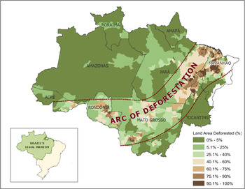
We calibrate the mathematical exercise above using data from the Brazilian Amazon. To represent a range of settlement histories, soil conditions and regions of the phase plane we use data from the states of Mato Grosso, Pará and Rondônia, which make up most of the ‘arc of deforestation’ or the region along the north and southwest border of the Legal Amazon (figure 2). This region was opened up as part of Operation Amazonia and populated through state-led settlement programs administered by the Brazilian land agency in the 1970s and 1980s. Poverty and inequality have decreased in recent decades for all states within the Brazilian Amazon (Guedes et al., Reference Guedes, VanWey, Hull, Antigo and Barbieri2014), while overall welfare has shown an upward trajectory (Caviglia-Harris et al., Reference Caviglia-Harris, Sills, Bell, Harris, Mullan and Roberts2014). The histories, migration rates and agricultural foci of these three states vary (de Espindola et al., Reference de Espindola, de Aguiar, Pebesma, Câmara and Fonseca2012; Bell et al., Reference Bell, Caviglia-Harris and Cak2015), although in all cases farming practices dictate that agricultural land is converted to pasture after several years and may ultimately be exhausted through continued use (although there is evidence to indicate otherwise; see Hall and Caviglia-Harris (Reference Hall and Caviglia-Harris2013) and VanWey et al. (Reference VanWey, Spera, de Sa, Mahr and Mustard2013)).
Map of the arc of deforestation

The state of Pará was largely settled by migrants from the northwest census region (one of the poorest in the nation) after a long drought. Land disputes and property turnover have been noted as major impediments to development in this state (Simmons, Reference Simmons2004; Ludewigs et al., Reference Ludewigs, D'Antona, Brondizio and Hetrick2009). Landowners in Pará tend to focus on perennial crops including, but not limited to cassava, peppercorn and sugarcane (Siegmund-Schultze et al., Reference Siegmund-Schultze, Rischkowsky, da Veiga and King2010). Mato Grosso first attracted investment by agricultural companies with interests in soy and cattle. As a result, landowners in this state tend to own large-scale mechanized soy and ranching operations with properties of more than 400 ha. In contrast, a large fraction of the landowners in Rondônia have small-scale farming and ranching operations (i.e., less than 200 ha) and have been successful in advancing the dairy and calving trades (Caviglia-Harris, Reference Caviglia-Harris2005). Soils in Mato Grosso and Pará tend to be relatively poor, classified as ‘average to restricted’ in their ability to support agriculture, while Rondônia has soils that are classified as some of the best in the Amazon and relatively ‘good’ for supporting agriculture (IBGE, 2014b).
5.2. Data
The data for parameterization originate from a variety of sources including the Brazilian Census Bureau (IBGE), the Brazilian Space Institute (INPE) and published estimates in academic articles. Together these data depict a transitional time period (table 1), with increasing real incomes and population and shifts in population from rural to urban areas between 1991 and 2010. Cattle herds increased within each of the three states, with the greatest growth observed in Rondônia. Finally, relative differences in geography are also included in table 1. Pará is the largest of the three states with more than five times the total land area of Rondônia and 1.4 times the land area of Mato Grosso.
Calibration data for model parameters: mean and total values by state (calculated from municipality-level data)

Notes: a Source: IBGE – Banco de Dados Agredados, ‘Tabela 200 – Populacão residente por sexo, situacão e grupos de idade – Amostra – Características Gerais da Populacão’, [available at] http://www.sidra.ibge.gov.br/bda/acervo/.
b Source: IBGE – Banco de Dados Agredados, ‘Tabela 2426 – Domicílios particulares permanentes, com rendimento domiciliar, Valor do rendimento nominal médio mensal’, [available at] http://www.sidra.ibge.gov.br/bda/acervo/.
c 1991 values are from state-level data (not calculated from the municipality-level data).
d Source: IBGE – Pesquisa Pecuária Municipal ‘Tabela 73 – Efetivo dos rebanhos, por tipo de rebanho (série encerrada)’, [available at] http://www.sidra.ibge.gov.br/bda/acervo/ (number of head includes cows, calves and bulls).
e Ranking is based on the ability to support agriculture: 1, good; 2, good–average; 3, average–good; 4, average; 5, average–restricted; 6, restricted; 7, restricted–unfavorable; 8, inadvisable. Source: IBGE (1992) ‘Mapa 1.19 Potencialidade Agricola dos Solos’ from the Atlas Nacional do Brasil; data downloaded from http://www.mmnt.net/db/0/0/geoftp.ibge.gov.br/mapas_interativos.
f Source: INPE, ‘PRODES Project: Monitoramento da Floresta Amazônica Brasileira por Satélite’ of the Brazilian Institute for Spatial Research, [available at] http://www.obt.inpe.br/prodes/index.php.
5.3. Results and sensitivity analysis
We begin by examining the case of Rondônia, which is illustrated as a phase diagram in figure 3a. The shape of the
 $\dot{l}_{A} =0$
isocline is different from the earlier diagrams because in this case published data suggest that the demand for agricultural goods is inelastic (Asano and Fiuza, Reference Asano and Fiuza2001; also see the appendix). Here, to the right of the
 $\dot{l}_{A} =0$
isocline, a large proportion of workers produce agricultural goods, the rural sector is relatively less profitable, and workers move into the urban sector. The
 $\dot{l}_{A} =0$
isocline swings down from the left to the rhs, intersecting the
 $\dot{s}=0$
isocline twice to form two interior steady states. These steady states are akin to points A and B in figures 1b and 1c. That is, the rightmost steady state is a stable equilibrium characterized by a large degree of soil productivity, although in this case most livelihoods are retained in the urban sector. The conditions of Rondônia suggest that the system will move to this interior equilibrium, with the model predicting that the population will become increasingly urban. This change has been observed historically; between 1991 and 2010 the rural population fraction declined from about 40 per cent to 26 per cent. If Rondônia was experiencing a collapse, the model predicts that agricultural productivity would be falling quickly, but this is not what has been observed in the state (Soler et al., Reference Soler, Verburg and Alves2014).
Phase diagrams of the model parameterized to three Brazilian states. (a) Rondônia, (b) Mato Grosso and (c) Pará

Next we consider the cases of Mato Grosso and Pará, which are illustrated in figures 3b and 3c, respectively. These outcomes are similar to the Rondônia case, although for Mato Grosso the model predicts a smaller share of rural population at the rightmost, stable equilibrium, which that state appears to be moving toward. The greater degree of separation between the Mato Grosso steady states suggests a relatively low risk of collapse. This outcome is attributable more to the relatively low population density of the state than to differences in soil quality. The model predicts that the Pará and Mato Grosso populations will become increasingly urban, but with a greater increase in Mato Grosso. Indeed, between 1991 and 2010 the rural population in Pará dropped from 48 per cent to 31 per cent and in Mato Grosso it dropped from 27 per cent to 18 per cent of the share of the total population.
Overall, the results suggest that ranching practices in this part of the frontier are sustainable, in the sense that exhaustion of the land and a collapse in regional incomes will not occur. Although a collapse scenario is not observed in the applications considered here, we can perform sensitivity analysis to gain insights into the plausibility of such an outcome. Specifically, we examine changes following 25 per cent increases and decreases in each parameter, ceteris paribus. We find that the Rondônia outcomes are sensitive to changes in soil dynamics: small increases in the soil loss rate (and decreases in the soil replenishment rate) lead to outcomes like that in figure 4, in which there is only the undesirable corner solution. On the other hand, the sensitivity analysis also suggests that the results are robust to changes in the economic parameters with the exception of the demand elasticities. Increases in the demand elasticity for agricultural output shift the
 $\dot{l}_{A} =0$
isocline up, making the conservation scenario less likely. This result would be reflective of the limited role that foodstuff prices play in agricultural output changes. Decreases in the demand elasticity for urban output also shift the
 $\dot{l}_{A} =0$
isocline up, because with small increases in labor, average urban income depresses significantly, discouraging movement out of the agricultural sector as soil productivity declines.
Results from a sensitivity analysis to the Rondônia case, with a higher rate of soil productivity loss compared with the benchmark

5.4. Population growth
Developing areas are known to face challenges from population growth through interregional migration and natural reproduction. The present model, by contrast, assumes a fixed labor market. Here we discuss how the outcomes of the Rondônia, Mato Gross and Pará applications would be affected by population growth.Footnote
6
First, consider the case of population growing continuously up to some exogenous limit. This would shift the
 $\dot{l}_{A} =0$
isocline up, which leaves open the possibility that with sufficient population growth the nullclines would no longer intersect. Now suppose the regional population is growing through immigration due to relatively high average incomes. This would shift the
 $\dot{l}_{A} =0$
isocline up, and the immigration rate would change as incomes adjust. Presumably, if the corner solution for a collapse materialized then emigration would occur, so that the
 $\dot{l}_{A} =0$
isocline would adjust downward until an interregional equilibrium is reached. Thus, significant population increases have the potential to lead an economy into collapse if the population growth is excessive.
6. Conclusions
Many resource-rich developing regions rely on agricultural production and the extraction of natural resources for economic development and growth. A counterintuitive result is that many of these nations end up with short-term gains while environmental and economic losses are the long-term result. While this development pattern has been adequately modeled in the past, the more recent steady growth of many of these nations provides the need for a framework that captures busts, growth and recovery based on resource extraction. This paper provides insight into factors that allow certain areas to develop successfully while others fail by introducing a model of agricultural productivity and soil quality that identifies several scenarios in which sustainable outcomes are achieved.
Our findings suggest that in the event of a collapse, temporary policies may successfully and permanently rehabilitate the agricultural sector and improve livelihoods in regions where soils are not extensively weak. This suggests that the emergence of an environmental and economic decline does not signal that a frontier area is unsuitable for agriculture. Instead, it may be the case that only small adjustments to local agricultural practices or economic conditions are necessary to promote sustainability. For example, strengthening off-farm employment opportunities (Reardon and Vosti, Reference Reardon and Vosti1995; Haggblade et al., Reference Haggblade, Hazell and Reardon2010) and supporting innovations in soil management (Scherr, Reference Scherr2000) could shield communities from negative resource shocks that would increase the risk of an environmental and economic collapse.
Our model calibration suggests that, contrary to concerns that agriculture-based development will lead to regional collapse, the examined areas in the frontier states of the Brazilian Amazon are on sustainable trajectories, although multiple equilibria may be present. Sensitivity analysis suggests that an economic and environmental collapse is a real risk in areas with higher erosion rates or poorer off-farm work opportunities compared with benchmark scenarios. Thus, while the environmental and economic costs of land degradation remain a serious concern, our application suggests that ranching-based agriculture in the Brazilian arc of deforestation will not cause a bust, and that Brazil's pursuit of agricultural development does not necessarily doom the country to the fate of consuming its tropical forests without long-run growth.
Appendix
This appendix details the calibration of the model. Agricultural and demographic census data on the Brazilian states of Rondônia and Mato Grosso were collected for 1991 (at the early stages of development) and in 2010 after much of the frontier was settled (table 1). For the baseline parameter values we use the data from 1991. For Rondônia, the maximum soil replenishment rate, r, was calculated based on maximum observed rates of 2 tons/ha (Pimentel et al., Reference Pimentel, Allen and Beers1987); with an area of 24 million ha this suggests r=48 million tons. The maximum soil level
 $\bar{S}$
was determined assuming that most soil nutrients lie in the top 20 cm, which contains the amount of 2,720 tons/ha of soil (Pimentel et al., Reference Pimentel, Allen and Beers1987); so for Rondônia
 $\bar{S} = 62,280$
(2,720×24) million tons. Next, the erosion parameter, δ, was calculated using an erosion rate on grazing lands of 6 tons/ha (Pimentel and Pimentel, Reference Pimentel and Pimentel2003); assuming this rate is observed after the removal of the first 10 cm of topsoil and with rural population of 470,000 in Rondônia, the loss parameter is determined by the formula
 $$6 \times 24 = \delta L_A /(0.5 \times \bar{S}) = \delta \times 470000/(0.5 \times 62280) \Rightarrow \delta = 9.5.$$
The agricultural production parameter, γ
A
, was calculated using a cattle herd size of about 3.26 million (cattle are the staple agricultural product in Rondônia), using the model formula for agricultural output,
 $3260000 = \gamma_{A} L_{A} S = \gamma_{A} \times 470000 \times (0.5 \times 62280)$
, which implies that
 $\gamma_{A} = 2.2 \times 10^{-4}$
. The elasticity of demand for agricultural products in Brazil is reportedly 1/2, so we use an inverse elasticity of demand
 $\varepsilon = 2$
(Asano and Fiuza, Reference Asano and Fiuza2001). In Rondônia, average rural income was about 5,500 Reais; we use this and the preceding figures to calculate the agricultural income scale factor, θ, as
 $$\theta = income \times L_A^{\varepsilon} /\gamma_A S = 5500 \times 470000^2 /(.00022 \times 0.5 \times 62280) = 1.8 \times 10^{14}.$$
The elasticity of demand for urban manufacturers in Brazil is about 1, so the inverse elasticity η=1 (Asano and Fiuza, Reference Asano and Fiuza2001). We normalize marginal urban output γ
U
to 1; thus with an urban population of 660,000 and an average urban income of 8,300, the urban income scale factor is
 $\varphi = income\times L_{U}^{\eta} = 8300 \times 660000^{1} = 5.5 \times 10^{9}$
.
The calibration procedures for Mato Grosso are akin to those used for Rondônia, although we leave the following parameters unchanged: δ=9.5, ε=2 and η=1. Otherwise, r=153 was calculated based on a maximum soil replenishment rate of 1.7 tons/ha (14 per cent reduction from Rondônia based on soil rankings in table 1) an area of 90 million ha. The maximum level of farmable soil is
 $\bar{S} = 244,800$
(2,720×90) million tons. As in Rondônia, the agricultural staple product in the state is cattle; with a herd size of 10 million, this implies γ
A
=1.6×10⁻⁴. With a rural population of 540,000 and an average income of about 6,300 Reais, the scale factor θ=9.4×10¹³. Having normalized γ
U
to 1, with an urban population of 1.49 million and an average urban income of 18,300, the scale factor φ=1.2×10¹⁰.
Likewise, for Pará we leave the following parameters unchanged: δ=9.5, ε=2 and η=1. However, r=240 was calculated based on a maximum soil replenishment rate of 1.9 tons/ha (4 per cent reduction from Rondônia), an area of 125 million ha. The maximum level of farmable soil is
 $\bar{S} = 340,000$
(2,720×90) million tons. With a herd size of about 7 million, this implies γ
A
=1.8×10⁻⁵. With a rural population of 2.35 million and an average income of about 23,000 Reais, the scale factor θ=4.2×10¹⁶. Having normalized γ
U
to 1, with an urban population of 2.6 million and an average urban income of 57,000, the scale factor φ=1.5×10¹¹.