

Introduction
Life course epidemiology seeks to understand the influence of several exposures across the life course, including in fetal life, on later health or disease risk.Reference Kuh, Ben-Shlomo, Lynch, Hallqvist and Power 1 Large-scale birth cohort studies provide a unique opportunity to model early life exposures in relation to later life outcomes. The implementation of life course models presents many methodological challenges for both the design and analysis of epidemiological studies.Reference Ben-Shlomo and Kuh 2 The primary goal of an analytical epidemiologic study is to obtain a valid and precise estimate of the effect of an exposure on an outcome. However, the internal validity of an estimate of a causal effect can be compromised by bias arising from confounding. Although confounding occurs in experimental research, it is a considerably more important issue in observational studies. Besides the general concept, some specific sources of confounding, including confounding by indication, confounding pattern altered by baseline selection, time-varying confounding and mediator–outcome confounding, are worth discussing in the context of life course epidemiology. Moreover, in this context, it is becoming increasingly common to combine individual-level data from several birth cohort studies in a meta-analysis, which offers advantages over the traditional aggregate data meta-analysis.Reference Riley, Lambert and Abo-Zaid 3 However, it remains unclear how the confounding should be addressed when data from different studies are centrally analyzed.
In this study, we first use directed acyclic graphs (DAGs) to briefly introduce the general concept of confounding. We then describe, provide examples and discuss specific sources of confounding that may play a relevant role in birth cohort studies: (i) confounding by indication, (ii) impact of baseline selection on confounding, (iii) time-varying confounding and (iv) mediator–outcome confounding. Finally, we discuss the issue of addressing confounding in the context of individual participant data meta-analyses.
Confounding
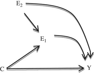
Confounding may be referred to as a ‘mixing of effects’ in which the effect of the exposure of interest on a given outcome is mixed with the effects of other factors resulting in a distortion of the true effect.Reference Rothman, Greenland and Lash 4 Confounding factors can overestimate or underestimate an effect, depending on the direction of their associations with exposure and outcome. The magnitude of confounding is of much greater importance than its mere presence or absence since it can hide a causal effect, falsely demonstrate an association where no causal association exists or even change the apparent direction of the effect estimate. Traditionally, for a variable to be a confounder, it must have three necessary (but not sufficient) characteristics: (1) it is a risk factor for the outcome conditional on the exposure; (2) it is associated with the exposure; and (3) it is not affected by the exposure or the outcome, in particular, it cannot be an intermediate step in the causal path between the exposure and the outcome.Reference Rothman, Greenland and Lash 4 Under the increasingly used graphical criteria, a confounder might be defined as a variable that should be used to block an otherwise open backdoor path. A backdoor path is a path from the exposure to the outcome that starts with an arrow pointing to the exposure. A collider is a variable which at least two arrows point to. A backdoor path is marginally blocked when contains a collider or is conditionally blocked when contains a non-collider on which it is conditioned (adjusted). Adjusting for a collider opens a path that was naturally blocked.Reference Rothman, Greenland and Lash 4 , Reference Greenland 5 Two potential scenarios are illustrated in Fig. 1, where E 1 and E 2 are the exposures of interest, Y the outcome and C a common cause of E 1 and Y. The DAG in Fig. 1 shows two backdoor paths from E 1 to Y (E 1–C–Y and E 1–E 2–Y), which are both marginally open (i.e., are not blocked before conditioning). Therefore, in order to estimate the effect of E 1 on Y, the analysis should condition on C and E 2. On the other hand, to estimate the effect of E 2 on Y the analysis does not need to condition on C or E 1 because there are no backdoor paths from E 2 to Y (i.e., no paths from E 2 to Y starting with an arrow pointing to E 2).
Directed acyclic graph representing confounding from E 1 to Y but not from E 2 to Y. E 1 and E 2 are the exposures, Y the outcome and C the confounder of E 1–Y association.

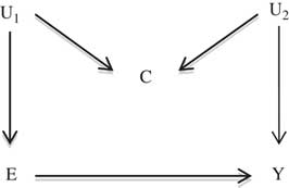
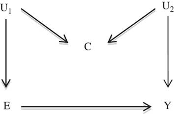
The traditional and graphical criteria for confounding usually lead to the same set of covariates for adjustment, and they both rely on external knowledge. For example, considering Fig. 1, both criteria indicate that C is a confounder of the effect of E 1 on Y. However, there are cases in which the traditional and the DAGs criteria disagree, and when that happens, it is the traditional criteria that fail, assuming that the graphical approach depicts correctly the underlying causal relationships among variables. A classical example, the so-called M-diagram,Reference Greenland 5 is illustrated in Fig. 2, where E is the exposure, Y the outcome, U 1 a common cause of E and C and U 2 a common cause of C and Y. In this DAG, C meets the three traditional criteria for a confounder since C is related to E and Y (by sharing a cause, U 1 and U 2, respectively), and it is not affected by E or Y. Based on the assumed causal structure, there is a backdoor path from E to Y that is blocked at C since C is a collider. Thus, no adjustment for C should be made; if C is adjusted for, the path becomes open and could only be blocked by conditioning on either U 1 or U 2. In the absence of data on U 1 and U 2, adjustment for C would introduce bias where none was present and lead to a potential spurious association between E and Y. An example of such scenario is a study that aims to evaluate the effect of breastfeeding (E) on later child’s obesity (Y), where maternal education (U 1) is related to both breastfeeding and maternal obesity (C) and mother’s genetic obesity risk (U 2) is related to both maternal obesity and child’s obesity (assuming that maternal education does not affect child’s obesity). Under these circumstances, maternal obesity would be identified as a confounder based on the traditional criteria but as a collider based on the graphical criteria. This reinforces why the traditional criteria might fail under some circumstances: every confounder must satisfy the traditional criteria but some non-confounders satisfy them as well.Reference Rothman, Greenland and Lash 4
Directed acyclic graph under which the traditional criteria fail to identify a confounder. E is the exposure, Y the outcome, and U 1 and U 2 the unmeasured confounders of E–C and C–Y association, respectively, and C the confounder of E–Y association based on the traditional, but not graphical, criteria.
Specific sources of confounding
Confounding by indication
Confounding by indication is a potentially severe form of confounding that arises when the indication for the treatment under study is a cause, or a consequence of a cause, of the outcome of interest.Reference Miettinen 6 , Reference Strom 7 For example, stage could confound a study on treatment for a given disease and overall mortality, or history of gastric problems could confound a study on use of anti-inflammatory drugs and gastric ulcer.Reference Strom 7 The latter example could also be labeled as confounding by contraindication.Reference Joseph, Mehrabadi and Lisonkova 8
In birth cohort research, confounding by indication may arise either for the child indication for the treatment or for maternal indication for the treatment during pregnancy or the periconceptional period. Figure 3a depicts a simple example of confounding by indication occurring when the child prognostic or risk factors for the disease of interest affect his/her likelihood of receiving the treatment. For example, in studies on exposure to antibiotics in infancy and asthma or lung function at school age, infant respiratory infections induce exposure to antibiotics and may increase the risk of asthma later in life.Reference van Meel, den Dekker and Elbert 9 To estimate the causal effect of antibiotics on asthma, it would be necessary to control for confounding by indication due to respiratory infections. One option would be to simply adjust for respiratory infections and another option would be to consider only exposure to antibiotics used for non-respiratory infections, thus breaking at least in part the indication pathway. Several other analytical options and design approaches are available.Reference McMahon 10 , Reference Garbe and Suissa 11
Directed acyclic graphs representing confounding by indication for (a) child’s treatment and (b) maternal treatment in birth cohort research.

The mechanism inducing confounding by indication is slightly more complex when the study focuses on exposure to a maternal treatment in pregnancy and a child health outcome. There is confounding by indication if the maternal characteristics that induce the treatment are associated with the child prognostic or risk factors for the disease under study. This usually happens through a backdoor path (Fig. 3b). For example, in a study on maternal use of antibiotics during pregnancy and asthma at school age, maternal respiratory tract infections during pregnancy could act as confounders by indication. Maternal respiratory infections induce the use of antibiotics and may be associated with the risk of child asthma, assuming that the increased maternal susceptibility to respiratory infections is associated with a similar child increased susceptibility to respiratory infections or asthma – the shared transmitted susceptibility is thus the reason for the open backdoor path.Reference Popovic, Rusconi and Zugna 12 In some instances, the maternal characteristics that induce the treatment directly affect child health, and the mechanism underlying confounding by indication becomes more similar to that depicted in Fig. 3a. For example, in a study of maternal use of antidepressant drugs in pregnancy and the risk of cardiac malformation, maternal conditions indicating for the use of antidepressants, including depression, sleep disorders, other mental health disorders, could cause cardiac malformations, for example, through their induced lifestyles (e.g., smoking). To control for confounding by indication in this scenario, in a large register-based study, analyses were restricted to mothers with a depression diagnosis and further stratified on a propensity score for the predicted probability of treatment.Reference Huybrechts, Palmsten and Avorn 13
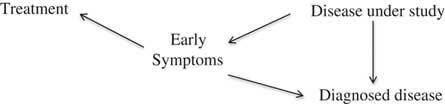
In case of child indication for the treatment, the terminology confounding by indication might be incorrectly used to indicate reverse causation or protopathic bias,Reference Horwitz and Feinstein 14 which occurs when the early manifestations of the outcome of interest induce the treatment.Reference Joseph, Mehrabadi and Lisonkova 8 , Reference Salas, Hofman and Stricker 15 In this scenario, the disease, through its symptoms, affects the medication and not vice-versa and thus the underlying causal mechanism is different from that of confounding (Fig. 4). It is of interest that this potential confusion between confounding by indication and reverse causation is less likely to occur when the exposure of interest is the maternal treatment in pregnancy, as in Fig. 3b: the indication for maternal treatment depends on maternal factors, and early manifestations of the child outcome cannot precede the exposure and introduce bias through reverse causation.
Directed acyclic graph representing protophatic bias in birth cohort research: the treatment is a consequence and not a cause of the outcome under study.

Treatments are prescribed with the intended aim of changing the natural history of a disease and prevent unfavorable outcomes (e.g., patients with respiratory infectious diseases are prescribed antibiotics to prevent death).Reference Miettinen 6 Treatments prescribed in a clinically appropriate manner are thus used more frequently by individuals with a high risk of having the outcome. For this reason, confounding by indication is particularly challenging, that is, the indication is strongly associated with both the treatment and the outcome. When it comes to side effects of the treatment, or the so-called unintended effects, especially when they are unknown or occur in the long term, the association between the indication and the outcome is expected to be weaker as the treatment is not prescribed specifically to prevent that outcome.Reference Miettinen 6 Let us consider an example of intended and unintended effects of use of antibiotics in pregnancy. Genitourinary infections in pregnancy are a strong indication for use of antibiotics and are strongly associated with the risk of adverse birth outcomes among the untreated women. An observational study on the use of antibiotics in pregnancy and adverse birth outcomes could find a positive association due to confounding by indication. In a study of use of antibiotics in pregnancy and child obesity, genitourinary infections would still be a strong indication for use of antibiotics, but their association with the outcome of interest (child obesity) among the untreated women would be much weaker. Confounding by indication could still introduce bias, but the magnitude of the bias would be smaller. Thus, confounding by indication is typically less problematic when the outcome of interest regards an unintended than an intended effect of the treatment. This has obvious positive implications for the validity of birth cohort research, which typically focuses on unintended long-term effects.
Impact of baseline selection on confounding
In birth cohort studies, participants can be either selected according to some prespecified criteria (intentional selection) and/or self-selected because of low baseline response rates or recruitment of volunteers (unintentional selection). It is widely acknowledged that baseline selection might alter the confounding pattern present in the general population,Reference Hernan, Hernandez-Diaz and Robins 16 – Reference Keiding and Louis 20 but there is still lack of clarity on the potential underlying mechanisms and on the consequences in terms of validity of the study results.
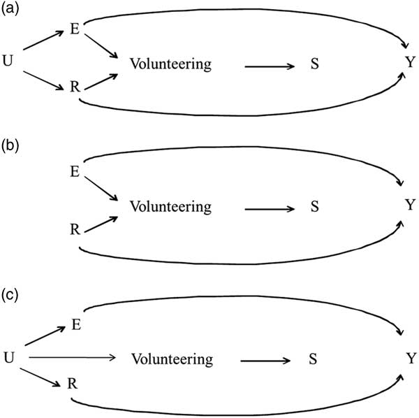
Baseline selection in birth cohorts, as well as in any cohort study, by definition cannot be affected by the outcome of interest. In this context, the confounding pattern of the general population can be altered if both the exposure of interest and another risk factor for the outcome are associated – either directly or through some other variables – with the probability of selection into the study. Some potential scenarios are illustrated in Fig. 5, where E indicates the exposure of interest, R a risk factor for the outcome Y, S an indicator of selection into the cohort and U is another unmeasured variable. Clearly modified/alternative versions of scenarios depicted in Fig. 5 exist and these scenarios are not mutually exclusive. Moreover, in the graphs for simplicity, we focus only on unintentional selection, but the same line of reasoning can be applied to the other selection mechanism.
Directed acyclic graphs of a birth cohort where subjects volunteer to participate. (a) In the general population, the exposure of interest (E) and the outcome risk factor (R) are associated as they share the common cause (U) and they both affect baseline selection (S) through volunteering. (b) E and R are independent in the general population and both affect the probability of selection through volunteering. (c) In the general population, E and R are associated because of the common cause (U), which, in turn, affects volunteering.

In the first situation (Fig. 5a), the exposure and the risk factor are associated in the general population because they share a common cause U and both affect the probability of being a volunteer. As a consequence, R is a confounder of the E–Y relationship, but among the study subjects, the E–R association is altered due to implicit conditioning on volunteering, which in Fig. 5a is a collider. Under this mechanism, baseline selection can either induce or attenuate the confounding effect of R depending on the strength and direction of the relationships involved (E-Volunteering, R-Volunteering, U–E, U–R).Reference Pizzi, De Stavola and Merletti 21 , Reference Glymour 22 An example of such scenario could be a study that aims to evaluate the effect of maternal consumption of antidepressant during pregnancy (E) on child neurodevelopment (Y), where both consumption of antidepressant and smoking during pregnancy (R) – a risk factor for the outcome of interest – are likely to decrease the probability of volunteering into the study. In the general population, we can assume that these two variables are positively associated due to the inverse association of maternal education (U) with both maternal consumption of antidepressant and smoking during pregnancy and therefore we can assume that positive confounding is present. As both smoking and consumption of antidepressant affect baseline selection in the same direction, we expect that among study participants a spurious negative association is induced between these two variables, thus attenuating the confounding present in the general population. An example with the same underlying mechanisms but with enlarged confounding bias due to baseline selection might be a study where parity (E) and smoking (R) negatively affect participation and are negatively associated in the general population due to maternal age (U), which is positively associated with parity and negatively with smoking during pregnancy.
In the second situation (Fig. 5b), the exposure and the risk factor still affect the likelihood of being a volunteer but are now independent in the general population. Restricting on S induces an association between E and R, making R a confounder among the study subjects. This is a type of collider bias that has been described extensively in the epidemiological literatureReference Greenland 5 , Reference Hernan, Hernandez-Diaz and Robins 16 – Reference Richiardi, Pizzi and Pearce 18 , Reference Pizzi, De Stavola and Merletti 21 , Reference Glymour 22 and that has been quantified also by simulation studies.Reference Pizzi, De Stavola and Merletti 21 An example of such scenario might be a study in which we want to evaluate the effect of maternal education (E) on reproductive outcomes (Y), where both maternal education and occurrence of previous miscarriages (R) affect the probability of participating into the study (S). Assuming that these two variables are independent in the time and place in which the study is conducted, when analyzing the birth cohort data, previous miscarriages become a confounder for the association between maternal education and reproductive outcomes.
Another special and relevant case is the one depicted in Fig. 5c, where the risk factor R is a confounder in the general population because it shares the common cause U with the exposure of interest E and the common cause is the factor influencing volunteering. Under this scenario, although there might be exceptions,Reference Ogburn and VanderWeele 23 typically the confounding bias present in the general population due to the E–U–R–Y backdoor path would be attenuated in the selected cohort because conditioning on S would imply a partial conditioning on U. This might be the case of a study on the effect of alcohol consumption during pregnancy (E) on child neurodevelopment (Y) with maternal education (U) influencing participation as well as alcohol consumption and maternal pre-pregnancy body mass index (BMI) (R), which we assume not to affect volunteering.
In all these scenarios, both in the general population and in the selected cohort, conditioning on R would block the backdoor path from E to Y and enhance valid scientific inference for the exposure–outcome effect. When R is unknown or unmeasured, confounding might be present both in the general population and in the selected birth cohort or in only one of the two depending on the underlying mechanisms involved, as baseline selection might induce but also reduce the confounding present in the general population. The bottom line is that the confounding pattern in the birth cohort may differ from that of the corresponding general population, both in terms of amount and direction of bias and in terms of relevant variables, we need to control for to minimize confounding, and efforts should be made to collect information on all known or potential relevant risk factors for the outcome of interest.
Time-varying confounding
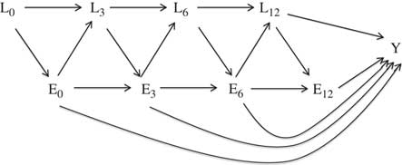
If the aim of a study is to estimate the causal effect of a time-varying exposure, that is, measured at different times for each subject, on an outcome, it is likely that time-varying confounders are present, that is, factors which change over time and confound the time-varying exposure–outcome causal relationship. The time-varying confounder affects the future exposure and predicts the outcome conditional on the past exposure. A simplified scenario with measured time-varying confounders and without further unmeasured and/or time-fixed confounders is represented in Fig. 6. The time-varying exposure is indicated by E t , t=0 , … , T, the time-varying confounder is indicated by L t , t=0, … , T, with L t occurring immediately before E t , and Y is the outcome of interest measured at a later time t>T. Let E t , t=0, 3, 6, 12, represents the breastfeeding measured at 24 h after birth, 3, 6 and 12 months, L t , t=0, 3, 6, 12, the infant’s weight at the same times and Y the infant’s wheezing at 18 months. Here, the infant’s weight can affect the current breastfeeding status and, at the same time, may be affected by the infant’s earlier breastfeeding status. Infant’s weight is both a confounder and a mediator of the relationship between breastfeeding and the risk of infant’s wheezing. In this framework, traditional modeling strategies cannot be used. Controlling only for infant’s weight measured at baseline (L 0) would produce a biased estimate of the causal effect of breastfeeding (E t , t=0, 3, 6, 12) on the risk of wheezing (Y) because it would ignore the fact that the breastfeeding over the first year of life (E t , t=3, 6, 12) depends on infants’ weight (L t , t=3, 6, 12), which, in turn, affects the risk of wheezing independently from breastfeeding. However, also controlling for time-varying measurements of infant’s weight (L t , t=0, 3, 6, 12) affected by prior breastfeeding would give a biased estimate of the causal effect of interest because breastfeeding (E t , t=0, 3, 6, 12) acts partly through the effect of infant’s weight (L t , t=3, 6, 12) on the outcome (Y).Reference Schisterman, Cole and Platt 24 Furthermore, in the presence of an unmeasured confounder of the time-varying confounders and the outcome association, controlling for time-varying measurements of the exposure would introduce a further source of collider biasReference Greenland 5 due to the induced spurious association between the exposure and the unmeasured confounder and consequently between the exposure and the outcome. Hence, there is the need for using alternative methods based on counterfactuals,Reference Hernán and Robins 25 , Reference Daniel, Cousens, De Stavola, Kenward and Sterne 26 such as inverse probability weighting,Reference Daniel, Cousens, De Stavola, Kenward and Sterne 26 – Reference Robins, Hernan and Brumback 28 G-formula computationReference Daniel, Cousens, De Stavola, Kenward and Sterne 26 , Reference Naimi, Cole and Kennedy 29 , Reference Taubman, Robins, Mittleman and Hernan 30 and g-estimation,Reference Daniel, Cousens, De Stavola, Kenward and Sterne 26 , Reference Naimi, Cole and Kennedy 29 , Reference Hernan, Cole, Margolick, Cohen and Robins 31 that adjust for confounding without blocking the effect of the exposure on the confounder.
Directed acyclic graph representing time-varying confounding. Y is the outcome, E t the time-dependent exposure and L t the time-dependent confounder of the E t –Y association.

Mediator–outcome confounding
Mediation analyses are traditionally performed by regressing the outcome on the exposure with and without the mediator.Reference Baron and Kenny 32 One common example is the adjustment for gestational age or weight at birth in studies aiming to assess the effect of maternal prenatal exposures on offspring outcomes. The estimate is interpreted as a total effect of the exposure on the outcome in the model unadjusted for the mediator and as a direct effect in the model adjusted for the mediator (i.e., the effect that is not mediated by the mediator included in the model). The difference between total and direct effects is the indirect effect (i.e., the effect that acts through the mediator included in the model). This traditional approach to mediation analyses may produce flawed conclusions due to four main sources of potential bias: (i) misclassification of the mediator,Reference Blakely, McKenzie and Carter 33 – Reference Ogburn and VanderWeele 36 (ii) the presence of exposure–mediator or exposure–confounders interaction and non-linearities,Reference Richiardi, Bellocco and Zugna 37 (iii) collider biasReference Greenland 5 , Reference Cole, Platt and Schisterman 38 might occur when adjusting for a mediator in the presence of unmeasured mediator–outcome confoundingReference Richiardi, Bellocco and Zugna 37 and (iv) a direct effect cannot be estimated if a variable that lies on the direct path between the exposure and the outcome confounds the mediator–outcome effect.Reference Richiardi, Bellocco and Zugna 37 Mediation approaches using counterfactual theory to estimate controlled and natural effects and approaches to sensitivity analyses have been developed, which address some of these limitations. These methods are beyond the scope of this review and have already been described elsewhere.Reference Richiardi, Bellocco and Zugna 37 , Reference VanderWeele 39 Here, we will discuss further the issue of mediator–outcome confounding and the special case when mediator–outcome confounding is affected by the exposure.
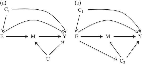
Suppose that we are interested in estimating the causal effect of an exposure on the outcome for a given level of the mediator (the controlled direct effect).Reference Richiardi, Bellocco and Zugna 37 , Reference Petersen, Sinisi and van der Laan 40 , Reference Pearl 41 In this context, not only we need to assume no unmeasured confounding of the exposure–outcome association but also we should assume absence of unmeasured confounding of the mediator–outcome association. We indicate the exposure by E, the mediator by M, the outcome by Y, the set of measured confounders of the E–Y association by C 1 and the unmeasured confounder of the M–Y association by U (Fig. 7a). An example of this scenario could be maternal BMI (E), breastfeeding duration (>6 months v. ⩽6 months) (M) and obesity at school age (Y), where U indicates the occurrence of infant’s infections in the first 6 months of life. The question of interest is how much of the effect of maternal BMI on the obesity at school age is mediated by breastfeeding duration, or in other words, the question is what would be the remaining effect of maternal BMI on the obesity at school age if all women breastfed for at least 6 months. As previously described, a common approach to address this question is to condition on breastfeeding duration (M), by stratifying the analyses on it or controlling for it in a regression model. However, conditioning on breastfeeding duration (a collider) (M) would induce a spurious association between maternal BMI (E) and occurrence of infant’s infections in the first 6 months of life (U),Reference Hernandez-Diaz, Schisterman and Hernan 42 , Reference VanderWeele, Mumford and Schisterman 43 opening the backdoor path maternal BMI–infant’s infections–obesity (E–U–Y), thus inducing a bias in the effect of interest. Hence, when estimating the controlled direct effect of an exposure on an outcome, traditional multivariable methods can be used if all confounders of mediator–outcome association are measured and are included in the analyses. Sensitivity analyses have been proposedReference VanderWeele 44 in order to quantify the bias in the presence of unmeasured/unknown mediator–outcome confounders. Suppose now that measured M–Y confounders (C 2) are affected by E (Fig. 7b), in which C 2 could be infant’s growth. Controlling for infant’s growth (C 2) to account for the spurious association induced by conditioning on breastfeeding (M) would give a biased estimate of the controlled direct effect because, in this way, the path from maternal BMI (E) to obesity at school age (Y) that goes through infant’s growth (C 2) would be blocked. In these circumstances, controlled direct effects can be consistently estimated using alternative methods based on counterfactuals, such as the inverse probability weightingReference Hernan, Brumback and Robins 27 , Reference Robins, Hernan and Brumback 28 and the G-formula computation,Reference Naimi, Cole and Kennedy 29 , Reference Taubman, Robins, Mittleman and Hernan 30 , Reference Daniel and De Stavola 45 that adjust for the effect of confounder on the M-Y association but not for the effect of exposure on the confounder. Further assumptions on absence of unmeasured/measured confounders are required when the aim is to estimate natural direct and indirect effects in a mediation analysis.Reference Petersen, Sinisi and van der Laan 40 , Reference Pearl 41
Directed acyclic graphs representing mediator–outcome confounding. Y is the outcome, E the exposure, M the mediator, C 1 the confounders of E–Y association, U the unmeasured confounder of the M–Y association and C 2 the measured confounder of the M–Y association affected by E.

Discussion
In this study, we described and discussed sources of confounding in birth cohort studies, provided some examples and referred to the methods that have been developed to tackle them. In most instances, multiple sources of confounding coexist, and each study has its specific confounding pattern. It is easy to conclude that confounding is one of the main challenges to causal inference in life course epidemiology. It is particularly relevant in the context of individual participant data meta-analyses of birth cohort studies.Reference Riley, Lambert and Abo-Zaid 3 Individual participant data meta-analyses on environmental exposures and genetic associations have already been published as part of birth cohort collaborations, such as CHICOS (http://www.chicosproject.eu/the-project/management/), EGG (http://egg-consortium.org/) and ENRIECO (http://www.enrieco.org/). These meta-analyses are commonly undertaken using the same set of confounders among all participating cohorts. This might be problematic if potential different confounding patterns, caused by different confounding structures in the population and/or baseline selection, are present. However, considering cohort-specific sets of covariates might be particularly difficult and time-consuming in an individual participant data meta-analysis comprising several cohorts. Also, adjustment for different covariates would complicate the use of one-stage models (i.e., individual level data from all studies are simultaneously analyzed in a multilevel model, taking into account clustering of participants within studies), limiting the analyses to two-stage models (i.e., individual-level data within a study are analyzed and subsequently, the results from each study are combined using conventional meta-analytical methods). Although both approaches can suffer from estimation challenges, the use of one-stage methods has been recommended.Reference Debray, Moons, Abo-Zaid, Koffijberg and Riley 46 Measures of heterogeneity and inconsistency across studies in a meta-analysis have been developed,Reference Higgins, Thompson, Deeks and Altman 47 and although a low value can support at least partly a little influence of confounding on the results, a high value is not necessarily indicative of different confounding patterns. Bias related to confounding might be indirectly evaluated by subgroup analyses of individual participant data (for instance, data from middle-income and high-income cohorts may be analyzed separately). Two-stage models considering a specific set of covariates per cohort might also be performed. Further research should focus on the impact of cohort-specific confounding in individual participant data meta-analyses.
Acknowledgments
None.
Financial support
This work was supported by the European Union’s Horizon 2020 research and innovation program under grant agreement 733206 (LifeCycle Project).
Conflicts of interest
None.