1 Introduction
The presence of multi-scale chaotic eddies is the key feature of turbulence, and the understanding of their precise origin and interactions has been the central challenge over many years. Perhaps, the most well-known multi-scale behaviour of turbulence is the Richardson–Kolmogorov energy cascade (Kolmogorov Reference Kolmogorov1941, Reference Kolmogorov1991) – production of turbulent kinetic energy takes place at the integral length scale of given fluid flow, and it is subsequently transported down to the smallest possible length scale, at which viscous force in the fluid dissipates the produced turbulent kinetic energy into heat. This feature, which arises essentially due to the interplay between inertial and viscous forces, forms the backbone of dissipation process in turbulence, although its classical scaling argument has recently been challenged (Vassilicos Reference Vassilicos2015).
When a turbulent flow is bounded by a solid surface (i.e. wall), the interplay between inertial and viscous forces appears to be developed in a much more complicated manner. In particular, the presence of the wall allows the viscous force to act directly on the mean shear, the origin of turbulence production in shear flows. Therefore, in wall-bounded shear flow, even energy-containing motions, which are the direct outcomes of turbulence production, emerge at multiple length scales, forming a highly complex topology of scale interaction and energy cascade. Such a complex flow topology is perhaps best described by the so-called ‘attached eddy’ hypothesis (Townsend Reference Townsend1976; Perry & Chong Reference Perry and Chong1982). In wall-bounded shear flow, the smallest energy-containing motions would be located in the near-wall region and scale in the inner unit, while the largest ones would extend over the entire wall-normal location with the length scale being the outer unit. In the intermediate region, the logarithmic mean velocity profile gradually develops with increasing Reynolds number, and the size of the energy-containing motions there is approximately proportional to distance from the wall.
Townsend (Reference Townsend1976) also hypothesized that the energy-containing eddies in wall-bounded turbulent shear flow (especially in the logarithmic region) are statistically self-similar, and subsequently made the seminal theoretical prediction that turbulence intensity of wall-parallel velocity components would exhibit the logarithmic wall-normal dependence. Further to the early refinement of the original theory (e.g. Perry & Chong Reference Perry and Chong1982; Perry, Henbest & Chong Reference Perry, Henbest and Chong1986; Perry & Marusic Reference Perry and Marusic1995), there has been a growing body of evidence that supports the attached eddy hypothesis, especially in recent years: for example, the logarithmic growth of near-wall streamwise turbulence intensity with the Reynolds number (Marusic Reference Marusic2001), the linear growth of spanwise integral length scale in the logarithmic region (Tomkins & Adrian Reference Tomkins and Adrian2003; del Álamo et al. Reference del Álamo, Jiménez, Zandonade and Moser2004), the observation of the logarithmic wall-normal dependence of turbulence intensity of wall-parallel velocity components (Jiménez & Hoyas Reference Jiménez and Hoyas2008; Marusic et al. Reference Marusic, Monty, Hultmark and Smits2013), the linearly growing eddy-turnover time scale in the logarithmic region (Lozano-Durán & Jiménez Reference Lozano-Durán and Jiménez2014; Hwang & Bengana Reference Hwang and Bengana2016) and the self-similar statistical behaviour in the logarithmic region (Hwang Reference Hwang2015; Mizuno Reference Mizuno2016; Baars, Hutchins & Marusic Reference Baars, Hutchins and Marusic2017). In particular, the self-similar statistical structure of the individual energy-containing eddies has recently been fully calculated by Hwang (Reference Hwang2015), who showed that each of these eddies is composed of an elongated streak and compact vortical structures statistically in the form of quasi-streamwise vortices.
With the growing recent evidence of the attached eddy hypothesis, it is also found that the sustainment of the individual energy-containing eddies in the hierarchy does not need any external energy input, as each bears a self-sustaining mechanism essentially independent of the motions at other scales (Jiménez & Pinelli Reference Jiménez and Pinelli1999; Hwang & Cossu Reference Hwang and Cossu2010b , Reference Hwang and Cossu2011; Hwang Reference Hwang2015; Hwang & Bengana Reference Hwang and Bengana2016). This feature is consistent with the so-called ‘outer-layer similarity hypothesis’ of Townsend (Reference Townsend1976), and has also been well supported by rough-wall experiments and simulations (e.g. Flores, Jiménez & del Álamo Reference Flores, Jiménez and del Álamo2007; Chung, Monty & Ooi Reference Chung, Monty and Ooi2014). Nevertheless, it should be emphasized that the existence of such a self-sustaining mechanism does not necessarily imply that the interactions between the energy-containing eddies are unimportant. In particular, such interactive processes appear to be very crucial in the near-wall region, to which all the energy-containing eddies in the hierarchy would contribute, to a certain extent: for example, the scale interaction between the wall-attached self-similar eddies was recently shown to play a crucial role in skin-friction generation at high Reynolds numbers (de Giovanetti, Hwang & Choi Reference de Giovanetti, Hwang and Choi2016).
Indeed, understanding of the interactions between the inner and outer structures has been an important issue of a large number of recent studies (Hutchins & Marusic Reference Hutchins and Marusic2007; Mathis, Hutchins & Marusic Reference Mathis, Hutchins and Marusic2009; Agostini, Touber & Leschziner Reference Agostini, Touber and Leschziner2014; Talluru et al. Reference Talluru, Baidya, Hutchins and Marusic2014; Agostini & Leschziner Reference Agostini and Leschziner2016; Agostini, Leschziner & Gaitonde Reference Agostini, Leschziner and Gaitonde2016, and many others). Most of them are focused on studying the near-wall region where the self-sustaining near-wall structures and the wall-reaching part of the outer structures are to interact. These studies often decompose the near-wall velocity field into the inner and outer components, and seek their mutual statistical relations to understand the superposition/modulation effect of the outer motion on the near-wall dynamics. Despite the important progress made by these studies, it should be pointed out that such a binary decomposition of the given near-wall velocity signal is not precisely compatible to the notion of the attached eddy hypothesis of Townsend (Reference Townsend1976), in which the near-wall velocity fluctuation is viewed as an outcome of collective influence of all the energy-containing eddies. Furthermore, it appears that the scale interaction not only involves the superposition/modulation effect, but also plays an important role in determining the near-wall scaling of the energy-containing eddies itself. Indeed, Hwang (Reference Hwang2016) has recently proposed that the near-wall penetration of the outer structure and its Reynolds-number-dependent peak wall-normal location result from a scale interaction process, which can be modelled by an inhomogeneous eddy viscosity in the wall-normal direction.
Given the emerging evidence on the existence of self-similar energy-containing eddies (attached eddy hypothesis), the issues of how the energy is transferred among them and of what would be the consequences of this now appear to be of crucial importance. The purpose of the present study is therefore to explore these issues with a particular emphasis on unveiling the inter-scale energy transfer in the logarithmic region where the eddies at almost all scales reside. Since the size of energy-containing motions is well characterized by their spanwise wavelength (e.g. Hwang Reference Hwang2015), we consider the equation of turbulent kinetic energy (TKE) for each spanwise Fourier mode. In this equation, the nonlinear turbulent transport term appears in the form of convolution between the spanwise Fourier modes (i.e. triadic wave interactions), and we will focus on complete visualization of the triadic interactions. It should be stressed that this approach should be able to unveil all the possible nonlinear interactions, such as energy cascade, energy transfer across different integral length scales and energy redistribution process among the velocity components, at least in a statistical manner. Indeed, we shall see that this approach has enabled us to make new observations, including energy cascade in terms of triadic wave interactions, the role of large energy-containing motions in the energy cascade of small energy-containing ones, and the existence of energy transfer from small to large scales that plays a crucial role in the formation of the wall-reaching part of the energy-containing motions in the log and outer regions (i.e. footprint).
2 Problem formulation
2.1 Equation for turbulent fluctuation revisited
We consider a turbulent flow in a plane channel. We denote by
 $x_{1}$
,
 $x_{2}$
and
 $x_{3}$
the streamwise
 $(x)$
, wall-normal
 $(y)$
and spanwise
 $(z)$
directions, respectively, and the corresponding velocity components by
 $u_{1}$
,
 $u_{2}$
and
 $u_{3}$
, which are also used interchangeably with
 $u$
,
 $v$
and
 $w$
. The height of the channel is given by
 $2h$
, and the lower and upper walls are located at
 $y=0$
and
 $y=2h$
, respectively. The standard Reynolds decomposition leads to the following equation for turbulent fluctuation:
 $$\begin{eqnarray}\frac{\unicode[STIX]{x2202}u_{i}^{\prime }}{\unicode[STIX]{x2202}t}+U_{j}\frac{\unicode[STIX]{x2202}u_{i}^{\prime }}{\unicode[STIX]{x2202}x_{j}}=-u_{j}^{\prime }\frac{\unicode[STIX]{x2202}U_{i}}{\unicode[STIX]{x2202}x_{j}}+\frac{\unicode[STIX]{x2202}\unicode[STIX]{x1D70F}_{ij}^{\prime }}{\unicode[STIX]{x2202}x_{j}},\end{eqnarray}$$
with
 $$\begin{eqnarray}\unicode[STIX]{x1D70F}_{ij}^{\prime }=-\frac{p^{\prime }}{\unicode[STIX]{x1D70C}}\unicode[STIX]{x1D6FF}_{ij}-(u_{i}^{\prime }u_{j}^{\prime }-\overline{u_{i}^{\prime }u_{j}^{\prime }})+\unicode[STIX]{x1D708}\frac{\unicode[STIX]{x2202}u_{i}^{\prime }}{\unicode[STIX]{x2202}x_{j}},\end{eqnarray}$$
where
 $i,j=1,2,3$
,
 $U_{i}=(U(y),0,0)$
is the mean velocity,
 $u_{i}^{\prime }$
the turbulent velocity fluctuation,
 $p^{\prime }$
the pressure fluctuation,
 $\unicode[STIX]{x1D70C}$
the fluid density,
 $\unicode[STIX]{x1D708}$
the kinematic viscosity and the overbar indicates the time average.
Before the equation for TKE of each spanwise Fourier mode is introduced, it is useful to discuss some features of (2.1). First, the left-hand side of (2.1a ) is a simple linear advection operator with the mean velocity. Therefore, it would mainly describe the downstream advection of turbulent velocity fluctuation with the local mean velocity (i.e. Taylor’s hypothesis), as also shown by del Álamo & Jiménez (Reference del Álamo and Jiménez2009) who directly calculated the advection velocities of turbulent fluctuation at different wall-normal locations. Indeed, the left-hand side of (2.1a ) is transformed into the advective transport term in the standard TKE equation (Pope Reference Pope2000), thereby not being directly involved in any TKE production.
Second, the first term on the right-hand side of (2.1a
) is directly transformed into the turbulence production term in the TKE equation: multiplying this term by
 $u_{i}^{\prime }$
and averaging it in time yields the standard turbulence production in parallel shear flow (i.e.
 $-\overline{u^{\prime }v^{\prime }}\text{d}U/\text{d}y$
). It should be realized that this term is from the linear part of (2.1) and that (2.1) itself turns out to be the linearized Navier–Stokes equation around the mean flow if the nonlinear term and the Reynolds stress in (2.1b
) are ignored. Furthermore, multiplying (2.1a
) by
 $u_{i}^{\prime }$
and integrating over the given control volume
 $\unicode[STIX]{x1D6FA}$
yields
 $$\begin{eqnarray}\frac{\text{d}}{\text{d}t}\int _{\unicode[STIX]{x1D6FA}}\frac{1}{2}u_{i}^{\prime }u_{i}^{\prime }\,\text{d}V=\int _{\unicode[STIX]{x1D6FA}}-u_{i}^{\prime }u_{j}^{\prime }\frac{\unicode[STIX]{x2202}U_{i}}{\unicode[STIX]{x2202}x_{j}}\,\text{d}V-\int _{\unicode[STIX]{x1D6FA}}\unicode[STIX]{x1D708}\frac{\unicode[STIX]{x2202}u_{i}^{\prime }}{\unicode[STIX]{x2202}x_{j}}\frac{\unicode[STIX]{x2202}u_{i}^{\prime }}{\unicode[STIX]{x2202}x_{j}}\,\text{d}V,\end{eqnarray}$$
where the first and second terms on the right-hand side are total turbulence production and dissipation, respectively. Since
 $\int _{\unicode[STIX]{x1D6FA}}u_{i}^{\prime }u_{i}^{\prime }\,\text{d}V$
is bounded in time, the left-hand side of (2.2) should vanish with time averaging, indicating the balance between the total production and dissipation. We also note that (2.2) is identical to the Reynolds–Orr equation in a flow instability problem, where
 $u_{i}^{\prime }$
and
 $U_{i}$
become finite-size disturbance and laminar base flow, respectively (Joseph Reference Joseph1976). In such a problem, the Reynolds–Orr equation has been used to emphasize the central role played by linear mechanisms in disturbance energy growth even in the nonlinear regime (Henningson Reference Henningson1996). In a similar manner, here one may argue that the TKE production in any turbulent shear flow should be mediated by linear mechanisms. This observation is also probably one of the reasons why a large number of previous linear analyses have been so useful for the description of coherent structures in both free (Ho & Huerre Reference Ho and Huerre1984) and wall-bounded shear flows (Butler & Farrell Reference Butler and Farrell1993; del Álamo & Jiménez Reference del Álamo and Jiménez2006; Cossu, Pujals & Depardon Reference Cossu, Pujals and Depardon2009; Pujals et al.
Reference Pujals, García-Villalba, Cossu and Depardon2009; Hwang & Cossu Reference Hwang and Cossu2010a
, and many others), even if the considered mean flows are not in the rapid-distortion limit.
Lastly, when the nonlinear and Reynolds stress terms in (2.1b ) are ignored, taking curl to (2.1a ) leads to the following equation:
 $$\begin{eqnarray}\frac{\unicode[STIX]{x2202}\unicode[STIX]{x1D714}_{y}^{\prime }}{\unicode[STIX]{x2202}t}+U\frac{\unicode[STIX]{x2202}\unicode[STIX]{x1D714}_{y}^{\prime }}{\unicode[STIX]{x2202}x}=-\frac{\unicode[STIX]{x2202}v^{\prime }}{\unicode[STIX]{x2202}z}\,\frac{\text{d}U}{\text{d}y}+\unicode[STIX]{x1D708}\unicode[STIX]{x1D6FB}^{2}\unicode[STIX]{x1D714}_{y}^{\prime },\end{eqnarray}$$
where
 $\unicode[STIX]{x1D714}_{y}^{\prime }$
is the wall-normal vorticity fluctuation. This equation is the Squire equation in physical space, and the first term on its right-hand side is the driving term, directly originating from the first term on the right-hand side of (2.1a
). We note that the driving term in (2.3) represents the so-called ‘lift-up’ effect, and it plays a key role in the generation of streaky motions (Butler & Farrell Reference Butler and Farrell1993; del Álamo & Jiménez Reference del Álamo and Jiménez2006; Cossu et al.
Reference Cossu, Pujals and Depardon2009; Pujals et al.
Reference Pujals, García-Villalba, Cossu and Depardon2009; Hwang & Cossu Reference Hwang and Cossu2010a
, and many others). This also implies that, in wall-bounded shear flows where inflection points are typically absent in the mean velocity profile, the lift-up effect should become a direct mechanism of turbulence production.
2.2 Equation for spectral TKE
Since the size of the energy-containing motions in wall-bounded turbulence is well characterized by the spanwise length scale (e.g. Hwang Reference Hwang2015), we first consider a Fourier-mode decomposition of turbulent velocity fluctuation in the spanwise direction:
 $$\begin{eqnarray}u_{i}^{\prime }(t,x,y,z)=\int _{-\infty }^{\infty }\widehat{u_{i}^{\prime }}(t,x,y,k_{z})\text{e}^{\text{i}k_{z}z}\,\text{d}k_{z},\end{eqnarray}$$
where
 $\,\widehat{\cdot }\,$
denotes the Fourier-transformed coefficient and
 $k_{z}$
is the spanwise wavenumber. We then take the Fourier transformation (2.4) to (2.1) and multiply it by
 $\widehat{u_{i}^{\prime }}^{\ast }(k_{z})$
(the superscript
 $^{\ast }$
denotes the complex conjugate). Taking the average in time and the streamwise direction yields
 $$\begin{eqnarray}\displaystyle \overline{\frac{\unicode[STIX]{x2202}\widehat{e}(k_{z})}{\unicode[STIX]{x2202}t}} & = & \displaystyle \underbrace{\left\langle \text{Re}\left\{-\overline{\widehat{u^{\prime }}^{\ast }(k_{z})\widehat{v^{\prime }}(k_{z})}\,\frac{\text{d}U}{\text{d}y}\right\}\right\rangle _{x}}_{\widehat{P}(y,k_{z})}+\underbrace{\left\langle -\unicode[STIX]{x1D708}\overline{\frac{\unicode[STIX]{x2202}\widehat{u_{i}^{\prime }}(k_{z})}{\unicode[STIX]{x2202}x_{j}}\frac{\unicode[STIX]{x2202}\widehat{u_{i}^{\prime }}^{\ast }(k_{z})}{\unicode[STIX]{x2202}x_{j}}}\right\rangle _{x}}_{\widehat{\unicode[STIX]{x1D700}}(y,k_{z})}\nonumber\\ \displaystyle & & \displaystyle +\,\underbrace{\left\langle \text{Re}\left\{-\overline{\widehat{u_{i}^{\prime }}^{\ast }(k_{z})\frac{\unicode[STIX]{x2202}}{\unicode[STIX]{x2202}x_{j}}(\widehat{\unicode[STIX]{x1D70F}_{ij,SGS}^{\prime }}(k_{z}))}\right\}\right\rangle _{x}}_{\widehat{\unicode[STIX]{x1D700}}_{SGS}(y,k_{z})}+\underbrace{\left\langle \text{Re}\left\{-\overline{\widehat{u_{i}^{\prime }}^{\ast }(k_{z})\frac{\unicode[STIX]{x2202}}{\unicode[STIX]{x2202}x_{j}}(\widehat{u_{i}^{\prime }u_{j}^{\prime }}(k_{z}))}\right\}\right\rangle _{x}}_{\widehat{T}_{turb}(y,k_{z})}\nonumber\\ \displaystyle & & \displaystyle +\underbrace{\left\langle \text{Re}\left\{\frac{\text{d}}{\text{d}y}\left(-\overline{\frac{\widehat{p^{\prime }}(k_{z})\widehat{v^{\prime }}^{\ast }(k_{z})}{\unicode[STIX]{x1D70C}}}\right)\right\}\right\rangle _{x}}_{\widehat{T}_{p}(y,k_{z})}+\underbrace{\left\langle \unicode[STIX]{x1D708}\frac{\text{d}^{2}\overline{\widehat{e}(k_{z})}}{\text{d}y^{2}}\right\rangle _{x}}_{\widehat{T}_{\unicode[STIX]{x1D708}}(y,k_{z})},\end{eqnarray}$$
where
 $\overline{\,\cdot \,}$
denotes the time average,
 $\langle \,\cdot \,\rangle _{x}$
the spatial average in the
 $x$
-direction,
 $\widehat{\unicode[STIX]{x2202}/\unicode[STIX]{x2202}x_{3}}=\text{i}k_{z}$
,
 $\widehat{e}(k_{z})=(|\widehat{u^{\prime }}(k_{z})|^{2}+|\widehat{v^{\prime }}(k_{z})|^{2}+|\widehat{w^{\prime }}(k_{z})|^{2})/2$
and
 $\text{Re}\{\,\cdot \,\}$
the real part. We note that
 $\unicode[STIX]{x1D70F}_{ij,SGS}^{\prime }$
in (2.5) is the subgrid-scale stress (SGS) fluctuation, and this is introduced here because the present study is based on a large-eddy simulation (LES) with an eddy-viscosity model (see also § 2.3). In (2.5), the left-hand side now turns out to be the rate of each spanwise Fourier mode of TKE, which should vanish in a statistically steady flow. The terms on the right-hand side are the rate of turbulence production, viscous dissipation, SGS dissipation, turbulent transport, pressure transport and viscous transport at a given spanwise wavenumber, respectively. Here, it is worth noting that all the linear terms on the right-hand side of (2.5), except the nonlinear term
 $\widehat{T}_{turb}$
, should only contain the given spanwise wavenumber
 $k_{z}$
due to their mathematical nature in the Fourier space, indicating that they do not involve any direct interactions between different scales. In contrast, the nonlinear term
 $\widehat{T}_{turb}(y,k_{z})$
, which represents the contribution of Reynolds stress transport to TKE at a given
 $k_{z}$
, involves interactions between multiple scales, as it can be written in the form of triadic wave interactions (see (3.1)). We note that, unless this term is written in the form of triadic wave interactions as in (3.1), it is difficult to gain any useful physical insight into scale interactions solely from this term in the form given in (2.5).
From (2.5), the standard TKE budget equation (Pope Reference Pope2000) is also obtained. Integration of (2.5) over the entire domain of spanwise wavenumber leads to
 $$\begin{eqnarray}0=\underbrace{-\overline{u^{\prime }v^{\prime }}\frac{\text{d}U}{\text{d}y}}_{P(y)}\underbrace{-\unicode[STIX]{x1D708}\overline{\left(\frac{\unicode[STIX]{x2202}u_{i}^{\prime }}{\unicode[STIX]{x2202}x_{j}}\right)^{2}}}_{\unicode[STIX]{x1D700}(y)}\;\underbrace{-\overline{u_{i}^{\prime }\frac{\unicode[STIX]{x2202}\unicode[STIX]{x1D70F}_{ij}^{\prime }}{\unicode[STIX]{x2202}x_{j}}}}_{\unicode[STIX]{x1D700}_{SGS}(y)}\;\underbrace{-\frac{\text{d}\overline{ev^{\prime }}}{\text{d}y}}_{T_{turb}(y)}\;\underbrace{-\frac{1}{\unicode[STIX]{x1D70C}}\,\frac{\text{d}\overline{p^{\prime }v^{\prime }}}{\text{d}y}}_{T_{p}(y)}\;\underbrace{+\unicode[STIX]{x1D708}\frac{\text{d}^{2}\bar{e}}{\text{d}y^{2}}}_{T_{\unicode[STIX]{x1D708}}(y)}.\end{eqnarray}$$
Here, we note that integration of each of the last three transport terms over the wall-normal domain results in zero. This indicates that all the transport terms in (2.5) should satisfy
 $$\begin{eqnarray}\displaystyle 2\int _{0}^{h}\int _{0}^{\infty }\widehat{T}_{turb}(y,k_{z})\,\text{d}k_{z}\,\text{d}y & = & \displaystyle 2\int _{0}^{h}\int _{0}^{\infty }\widehat{T}_{p}(y,k_{z})\,\text{d}k_{z}\text{d}y\nonumber\\ \displaystyle & = & \displaystyle 2\int _{0}^{h}\int _{0}^{\infty }\widehat{T}_{\unicode[STIX]{x1D708}}(y,k_{z})\,\text{d}k_{z}\text{d}y=0,\end{eqnarray}$$
and, equivalently,
 $$\begin{eqnarray}\displaystyle & & \displaystyle 2\int _{-\infty }^{logh}\int _{-\infty }^{\infty }~k_{z}y\widehat{T}_{turb}(y,k_{z})\,\text{d}\text{log}\,k_{z}\,\text{d}\text{log}\,y=2\int _{-\infty }^{logh}\int _{-\infty }^{\infty }k_{z}y\widehat{T}_{p}(y,k_{z})\,\text{d}\text{log}\,k_{z}\,\text{d}\text{log}\,y\nonumber\\ \displaystyle & & \displaystyle \quad =2\int _{-\infty }^{logh}\int _{-\infty }^{\infty }k_{z}y\widehat{T}_{\unicode[STIX]{x1D708}}(y,k_{z})\,\text{d}\text{log}\,k_{z}\,\text{d}\text{log}\,y=0.\end{eqnarray}$$
Finally, it should be mentioned that the analysis given here may also be performed with streamwise Fourier modes of turbulent fluctuation. However, given the statistical structure of the energy-containing motions at each scale (Hwang Reference Hwang2015), such an analysis does not appear to be particularly useful to understand the interactions between the energy-containing motions at different scales. Indeed, the self-sustaining energy-containing motion at a given spanwise length scale
 $\unicode[STIX]{x1D706}_{z}$
was previously found to be composed of two structures, i.e. an elongated streak and streamwise vortical structures (Hwang Reference Hwang2015). The former has a long streamwise extent characterized by
 $\unicode[STIX]{x1D706}_{x}\simeq 10\unicode[STIX]{x1D706}_{z}$
, whereas the latter is only
 $\unicode[STIX]{x1D706}_{x}\simeq 2-3\unicode[STIX]{x1D706}_{z}$
. These two elements are dynamically interconnected and they are known to form self-sustaining process. Therefore, the spectral energy transfer between the streamwise Fourier modes would include not only the inter-scale process (like scale interactions) but also the intra-scale one (like self-sustaining process), resulting in a difficulty to distinguish one from another. For example,
 $\unicode[STIX]{x1D706}_{x}^{+}\simeq 1000$
indicates near-wall streaks in the near-wall region, but the vortical structures at
 $\unicode[STIX]{x1D706}_{z}^{+}\simeq 500$
in the logarithmic region have the same streamwise length scale from
 $\unicode[STIX]{x1D706}_{x}\simeq 2-3\unicode[STIX]{x1D706}_{z}$
. However, this difficulty does not arise with the spanwise Fourier mode, as demonstrated by the numerical experiment in Hwang (Reference Hwang2015).
2.3 Numerical method and verification
In the present study, an LES is conducted by imposing a constant mass flux across the channel. The wall-normal velocity and vorticity form of the Navier–Stokes equation is integrated, as in Kim, Moin & Moser (Reference Kim, Moin and Moser1987). For the spatial discretization, the Fourier–Galerkin method is used in the
 $x$
- and
 $z$
-directions with dealiasing, and the Chebychev-tau method is used in the
 $y$
-direction. The time advancement is accomplished using a second-order semi-implicit scheme: a second-order Crank–Nicolson method for the diffusion terms and a third-order Runge–Kutta method for the convection terms. For the SGS model, a dynamic global eddy-viscosity model (Park et al.
Reference Park, Lee, Lee and Choi2006; Lee, Choi & Park Reference Lee, Choi and Park2010) is utilized. The computation is carried out in the domain size of
 $8\unicode[STIX]{x03C0}h(x)\times 2h(y)\times \unicode[STIX]{x03C0}h(z)$
with the number of grid points of
 $512(x)\times 145(y)\times 128(z)$
(after dealiasing). The resulting grid spacings are
 $\unicode[STIX]{x0394}x^{+}=82$
,
 $\unicode[STIX]{x0394}y^{+}=0.4-36.4$
and
 $\unicode[STIX]{x0394}z^{+}=41$
(the superscript
 $^{+}$
indicates the inner-scaled variables). The Reynolds number of the present LES is
 $Re_{\unicode[STIX]{x1D70F}}(\equiv u_{\unicode[STIX]{x1D70F}}h/\unicode[STIX]{x1D708})=1672$
, where
 $u_{\unicode[STIX]{x1D70F}}$
is the wall shear velocity.
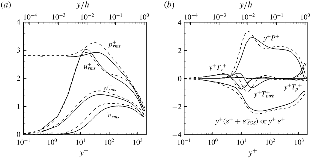
Turbulence statistics: (a) root-mean-square velocity and pressure fluctuations; (b) turbulent kinetic energy budget. ——, Present LES; – – –, DNS at
 $Re_{\unicode[STIX]{x1D70F}}=1995$
(Lee & Moser Reference Lee and Moser2015b
).
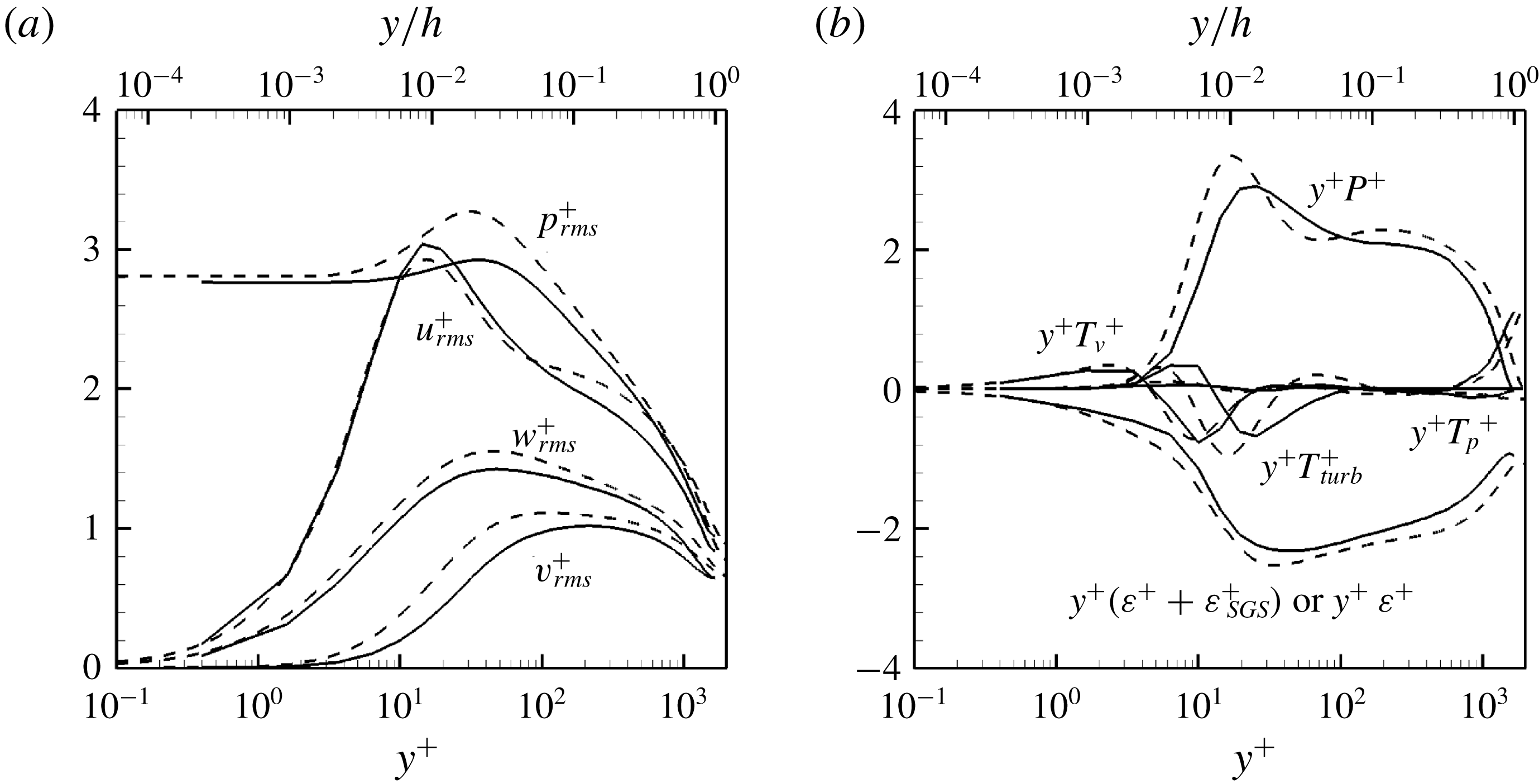
Figure 1 compares turbulent statistics of the present LES at
 $Re_{\unicode[STIX]{x1D70F}}=1672$
with those of direct numerical simulation (DNS) at
 $Re_{\unicode[STIX]{x1D70F}}=1995$
by Lee & Moser (Reference Lee and Moser2015b
). The root-mean-square (rms) velocity and pressure fluctuations show good agreement with those of DNS (figure 1
a). The constituents of (2.6) are also compared in figure 1(b). Here, since the present LES is based on a dissipative SGS model, the viscous dissipation from the DNS is compared with sum of the viscous dissipation and SGS dissipation. All constituents of the balance equation agree reasonably well with those from the DNS. It should be noted that the difference between the present LES and DNS does not change the results in the present study, in the sense that all the qualitative features from DNS are recovered by the present LES (see § 3.1 for further details).
3 Results
3.1 One-dimensional spectra
The constituents in the spectral TKE budget equation (2.5) have recently been computed by Lee & Moser (Reference Lee and Moser2015a ) and Mizuno (Reference Mizuno2016). Therefore, we start this section only by briefly reporting them in figure 2. Overall, the spectra of the present LES qualitatively capture all the important features reported by the previous DNS studies (Lee & Moser Reference Lee and Moser2015a ; Mizuno Reference Mizuno2016), except for very high spanwise wavenumbers, at which the present simulation would exhibit lack of resolution. However, this is not a great limitation of the present study, as the main scope of the present study is to explore interactions between ‘energy-containing’ motions and the region of high spanwise wavenumbers is mostly related to the classical energy cascade. Furthermore, the resolution of the present LES does not appear to be particularly bad either, as it covers the Kolmogorov length scale in the dissipation range at least to some extent (see also figure 2 b).
Premultiplied one-dimensional spanwise wavenumber spectra: (a) production
 $(Re_{\unicode[STIX]{x1D70F}}k_{z}y\widehat{P}^{+})$
; (b) viscous dissipation
 $(Re_{\unicode[STIX]{x1D70F}}k_{z}y\widehat{\unicode[STIX]{x1D700}}^{+})$
; (c) SGS dissipation
 $(Re_{\unicode[STIX]{x1D70F}}k_{z}y\widehat{\unicode[STIX]{x1D700}}_{SGS}^{+})$
; (d) turbulent transport
 $(Re_{\unicode[STIX]{x1D70F}}k_{z}y\widehat{T}_{turb}^{+})$
; (e) pressure transport
 $(Re_{\unicode[STIX]{x1D70F}}k_{z}y\widehat{T}_{p}^{+})$
; (f) viscous transport
 $(Re_{\unicode[STIX]{x1D70F}}k_{z}y\widehat{T}_{\unicode[STIX]{x1D708}}^{+})$
. Here, the production and dissipation spectra are energetic along
 $\unicode[STIX]{x1D706}_{z}=5y$
and
 $57\unicode[STIX]{x1D702}$
, respectively.
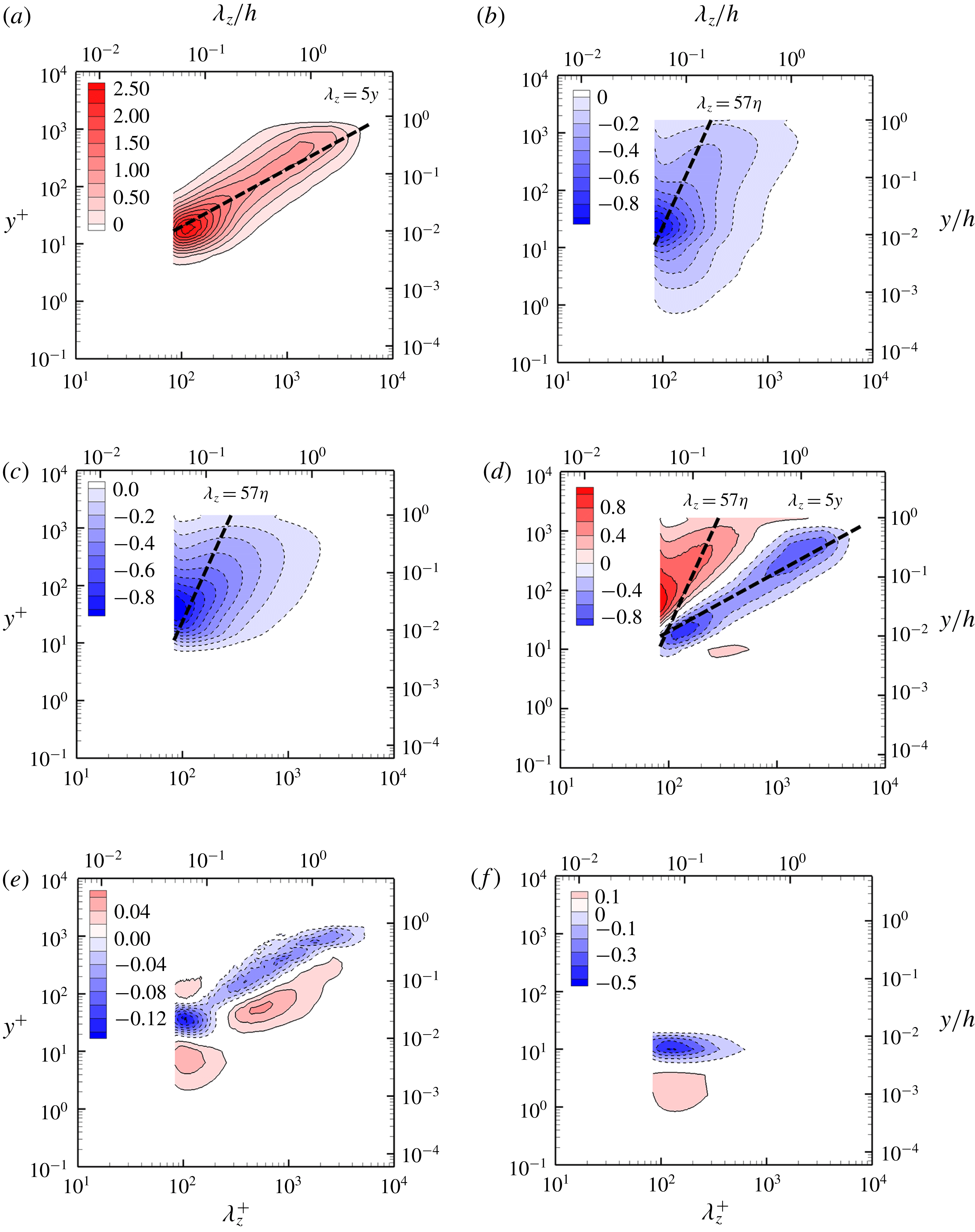
Figure 2(a) shows one-dimensional spanwise wavenumber spectra of turbulent production. Here, the spectra are premultiplied by
 $k_{z}$
and
 $y$
to represent their spectral intensity in logarithmic axes (see (2.8)). The turbulent production spectra appear to be almost uniformly distributed along
 $\unicode[STIX]{x1D706}_{z}=5y$
, especially over the range of the spanwise wavelength associated with the log layer (
 $300\unicode[STIX]{x1D6FF}_{\unicode[STIX]{x1D708}}\lesssim \unicode[STIX]{x1D706}_{z}\lesssim 1h$
in figure 2(a) where
 $\unicode[STIX]{x1D6FF}_{\unicode[STIX]{x1D708}}=\unicode[STIX]{x1D708}/u_{\unicode[STIX]{x1D70F}}$
). This indicates that the turbulence production at each scale is roughly identical throughout the log region. The spectra are also well aligned along the dashed-lined linear ridge
 $\unicode[STIX]{x1D706}_{z}=5y$
, consistent with the attached eddy hypothesis (Townsend Reference Townsend1976).
The spectra of viscous and SGS dissipation are reported in figures 2(b) and 2(c), respectively. The dashed line in these figures is
 $\unicode[STIX]{x1D706}_{z}=57\unicode[STIX]{x1D702}$
, where
 $\unicode[STIX]{x1D702}$
is the Kolmogorov length scale with the dissipation rate
 $\unicode[STIX]{x1D700}=u_{\unicode[STIX]{x1D70F}}^{3}/(\unicode[STIX]{x1D705}y)$
(
 $\unicode[STIX]{x1D705}$
is the Kármán constant set to be
 $\unicode[STIX]{x1D705}$
=0.41). We note that this dissipation rate is derived using the production in the logarithmic region, and it would be a reasonable first approximation at least roughly between
 $y^{+}\simeq 50$
and
 $y/h\simeq 0.2$
. The viscous dissipation spectra are reasonably well aligned with
 $\unicode[STIX]{x1D706}_{z}=57\unicode[STIX]{x1D702}$
, although the small-scale eddies associated with turbulent dissipation are not supposed to be fully resolved by the present LES (figure 2
b) (note that the typical size of the eddies at the Kolmogorov microscale is only
 $O(\unicode[STIX]{x1D702})$
(Jiménez & Wray Reference Jiménez and Wray1998)).
Unlike the production and dissipation spectra, the premultiplied transport spectra in figure 2(d–f) have energy gain (red) and loss (blue) due to their nature in (2.8). Given the relatively high Reynolds number in the present study, the dominant mechanism of energy transfer across the scales would be turbulent transport especially in the log and outer regions, where the values of its spectra are much larger than those of pressure and viscous transport spectra. Throughout the log and outer regions, the turbulent transport spectra exhibit large negative values along
 $\unicode[STIX]{x1D706}_{z}=5y$
, which are comparable to those of the positive counterpart in the production spectra (figure 2
a). This suggests that the main role played by turbulent transport in the log and outer regions is to transfer most of the TKE produced at the integral length scales to the other scales, at which the turbulent transport spectra are positive (figure 2
d). There are two regions of positive turbulent transport spectra, one of which appears in
 $\unicode[STIX]{x1D706}_{z}<5y$
and the other is in
 $\unicode[STIX]{x1D706}_{z}>5y$
. In the former region, both the viscous and SGS dissipation spectra exhibit large negative values (figure 2
b,c), indicating that the related turbulent transport mechanism is the Richardson–Kolmogorov energy cascade. Indeed, it was recently shown that the DNS data of Lee & Moser (Reference Lee and Moser2015b
) exhibit the typical inertial range spectra (i.e.
 $k_{z}^{-5/3}$
law) in this region (see also Agostini, Leschziner & Gaitonde Reference Agostini, Leschziner and Gaitonde2017). In the DNS data of Lee & Moser (Reference Lee and Moser2015a
), the negative dissipation spectra also well extend to the near-wall region, indicating that the energy cascade is also the primary turbulent transport mechanism in this region. In the present LES where this near-wall dissipation cannot be properly resolved, this energy cascade in the near-wall region is mainly replaced by SGS dissipation. In the latter region, the emergence of positive turbulent transport spectra is a little surprising, as it is not expected from the view of classical energy cascade. The emergence of weak positive turbulent transport spectra in the near-wall region was also reported by previous DNS studies (Lee & Moser Reference Lee and Moser2015a
; Mizuno Reference Mizuno2016), and this has been speculated to represent the near-wall modulation of large-scale structures (Lee & Moser Reference Lee and Moser2015a
). However, we shall later see that this is actually associated with turbulent transport from smaller scales (see figure 8). It is also important to point out that, despite the small values of the spectra in this region, the related turbulent transport cannot be simply ignored because the premultiplication factors (
 $k_{z}$
and
 $y$
) for the turbulent spectra in figure 2 are given to highlight the contribution to the global turbulent transport. This part of positive turbulent transport can certainly have an important local effect on the near-wall region where scale interactions would be highly active. Indeed, in § 4.2, we shall see that the positive turbulent transport plays a crucial role in the formation of the near-wall TKE spectra. Finally, the pressure and viscous spectra are found to be very small in the log and outer regions (see the contour legends in figure 2
e,f). In the near-wall region, the viscous transport spectra are important, but their importance is limited only for
 $y^{+}\lesssim 20$
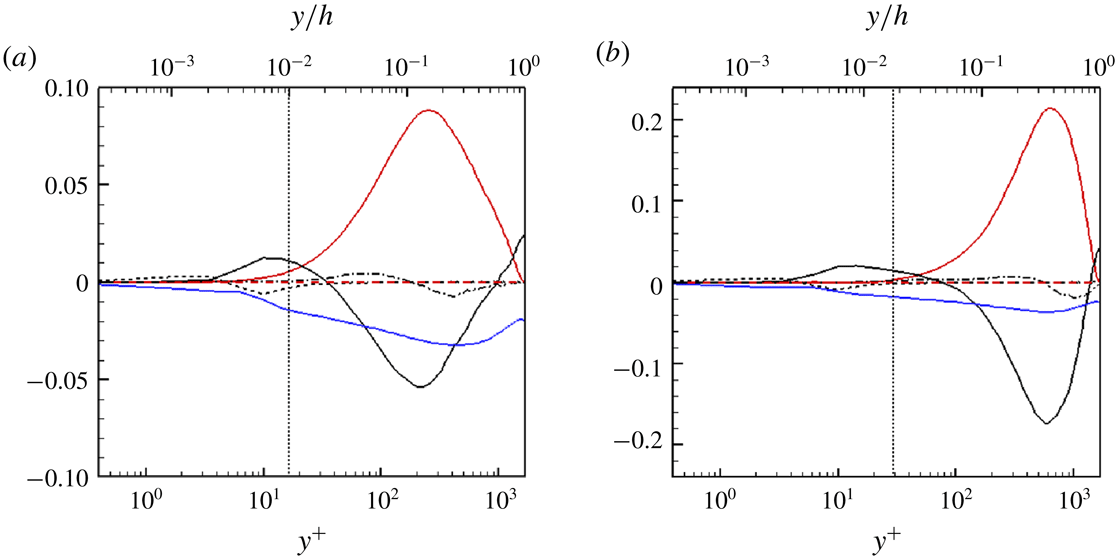
as is
 $T_{\unicode[STIX]{x1D708}}(y)$
in figure 1(b) (see also figure 13).
3.2 Triadic interactions and nonlinear energy transfer
Now, to understand the precise origin of the turbulent transport,
 $\widehat{T}_{turb}$
in (2.5) is written in the following form of the discretized convolution:
 $$\begin{eqnarray}\widehat{T}_{turb}(y,k_{z,0})=\left\langle \text{Re}\left\{-\overline{\widehat{u_{i}^{\prime }}^{\ast }(y,k_{z,0})\frac{\unicode[STIX]{x2202}}{\unicode[STIX]{x2202}x_{j}}\mathop{\sum }_{l+m=k_{z,0}}\widehat{u_{i}^{\prime }}(y,l)\widehat{u_{j}^{\prime }}(y,m)}\right\}\right\rangle _{x},\end{eqnarray}$$
where
 $l$
and
 $m$
are the spanwise wavenumbers for the convolution sum. The turbulent transport spectrum at the given spanwise wavelength
 $\unicode[STIX]{x1D706}_{z,0}(=2\unicode[STIX]{x03C0}/k_{z,0})$
and the wall-normal location
 $y$
is represented by triadic wave interactions between the spanwise Fourier modes of the wavenumbers
 $l$
and
 $m(=k_{z,0}-l)$
. Since the Fourier transform here is taken for real variables, the Fourier coefficients for negative wavenumbers correspond to complex conjugate of the ones for positive wavenumbers. Therefore, for positive
 $k_{z,0}$
, the convolution in (3.1) is written as
 $$\begin{eqnarray}\displaystyle \mathop{\sum }_{l+m=k_{z,0}}\widehat{u_{i}^{\prime }}(l)\widehat{u_{j}^{\prime }}(m) & = & \displaystyle \mathop{\sum }_{\substack{ l+m=k_{z,0} \\ l,m\geqslant 0}}\widehat{u_{i}^{\prime }}(l)\widehat{u_{j}^{\prime }}(m)\nonumber\\ \displaystyle & & \displaystyle +\,\mathop{\sum }_{\substack{ -l+m=k_{z,0} \\ l,m\geqslant 0}}\widehat{u_{i}^{\prime }}(-l)\widehat{u_{j}^{\prime }}(m)+\mathop{\sum }_{\substack{ l-m=k_{z,0} \\ l,m\geqslant 0}}\widehat{u_{i}^{\prime }}(l)\widehat{u_{j}^{\prime }}(-m),\end{eqnarray}$$
indicating that
 $\widehat{T}_{turb}(y,k_{z,0})$
in this case can be represented over
 $l+m=k_{z,0}$
,
 $l-m=k_{z,0}$
and
 $-l+m=k_{z,0}$
in the first quadrant of the
 $l$
–
 $m$
plane (i.e.
 $l,m\geqslant 0$
; see also figure 6
a). Furthermore, (3.1) implies
 $$\begin{eqnarray}\widehat{T}_{turb}(y,-k_{z,0})=\widehat{T}_{turb}^{\ast }(y,k_{z,0})=\widehat{T}_{turb}(y,k_{z,0}).\end{eqnarray}$$
Therefore, the case of negative
 $k_{z,0}$
is not considered separately.
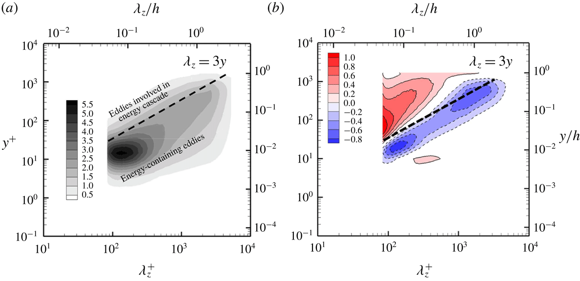
Premultiplied one-dimensional spanwise wavenumber spectra: (a) turbulent kinetic energy,
 $\widehat{e}(y,k_{z})$
; (b) turbulent transport,
 $\widehat{T}_{turb}(y,k_{z})$
. Here,
 $\unicode[STIX]{x1D706}_{z}=3y$
is a boundary that distinguishes between the energy-containing eddies and the ones related to energy cascade.

Although (3.1) enables us to examine all the triadic interactions between the spanwise Fourier modes, it should be reminded that each of these Fourier modes resolves not only the energy-containing eddies but also the ones generated by energy cascade. Therefore, it would be useful to distinguish the part of each Fourier mode representing the energy-containing eddies from the rest that would indicate the eddies involved in energy cascade. For this purpose, we further examine one-dimensional spanwise wavenumber spectra of turbulent kinetic energy and turbulent transport, as shown in figure 3. The TKE spectra contain most of energy for
 $\unicode[STIX]{x1D706}_{z}>3y$
(figure 3
a). Furthermore, in this region, the turbulent transport spectra are mostly negative (figure 3
b), suggesting that
 $\unicode[STIX]{x1D706}_{z}=3y$
would be considered as a reasonable boundary that distinguishes between the energy-containing eddies and the ones related to energy cascade in the spanwise wavenumber spectra. In other words, for a given spanwise Fourier mode with the wavelength
 $\unicode[STIX]{x1D706}_{z,0}$
, the wall-normal profile with
 $y<\unicode[STIX]{x1D706}_{z,0}/3$
would mainly resolve the energy-containing eddies, while the rest given by
 $y>\unicode[STIX]{x1D706}_{z,0}/3$
would capture the motions involved in energy cascade.
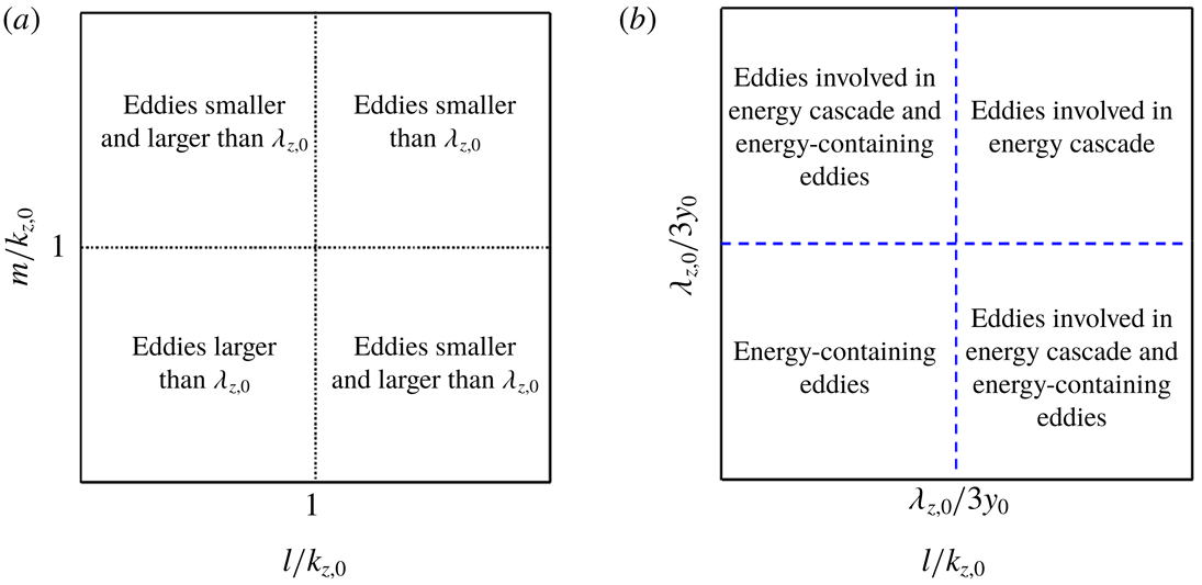
Classifications of the origin of turbulent transport based on (a) the spanwise wavelength of the eddies relative to that of the given Fourier mode
 $(\unicode[STIX]{x1D706}_{z,0})$
and (b) the nature of eddies (i.e. energy-containing ones or the ones involved in energy cascade).

This setting now allows us to more precisely understand the origin of turbulent transport for given
 $k_{z,0}$
and
 $y$
based on the size and nature of the eddies involved in the triadic interactions. Figure 4(a) describes a classification of the triadic interactions for turbulent transport in the
 $l$
–
 $m$
plane based on the spanwise size of the eddies relative to that of the given Fourier mode (
 $\unicode[STIX]{x1D706}_{z,0}(=2\unicode[STIX]{x03C0}/k_{z,0})$
). We first normalize the
 $l$
and
 $m$
axes by
 $k_{z,0}$
, and divide the
 $l$
–
 $m$
plane into four regions with
 $l/k_{z,0}=m/k_{z,0}=1$
. Any combinations of
 $l$
and
 $m$
emerging in the right-upper region (
 $l,m>k_{z,0}$
) for
 $\widehat{T}_{turb}(y,k_{z,0})$
are then identified to originate from the interactions between the eddies, the spanwise size of which is smaller than
 $\unicode[STIX]{x1D706}_{z,0}$
(see also figure 6 for application of this classification). On the other hand, those given in the lower-left region (
 $l,m<k_{z,0}$
) are from the interactions of the eddies larger than
 $\unicode[STIX]{x1D706}_{z,0}$
. In the remaining two regions, the combinations of
 $l$
and
 $m$
for
 $\widehat{T}_{turb}(y,k_{z,0})$
are from a pair of the eddies, one of which has larger spanwise wavelength than
 $\unicode[STIX]{x1D706}_{z,0}$
and the other does not. In a similar manner, the origin of turbulent transport can also be classified in the
 $l$
–
 $m$
plane based on the nature of the eddies (i.e. energy-containing eddies versus eddies generated by energy cascade), as described in figure 4(b). The two blue dashed lines in figure 4(b) are
 $l=2\unicode[STIX]{x03C0}/(3y_{0})$
and
 $m=2\unicode[STIX]{x03C0}/(3y_{0})$
, respectively, and they are given from
 $\unicode[STIX]{x1D706}_{z}=3y$
in figure 3 (i.e.
 $y_{0}=\unicode[STIX]{x1D706}_{z,0}/3$
). These lines also divide the
 $l$
–
 $m$
plane into four regions. In this case, the combinations of
 $l$
and
 $m$
given in the right-upper region (
 $l,m>2\unicode[STIX]{x03C0}/(3y_{0})$
) are from the triadic interactions between the eddies generated by energy cascade, whereas those in the left-lower region (
 $l,m<2\unicode[STIX]{x03C0}/(3y_{0})$
) are from the interactions between the energy-containing eddies. In the remaining two regions, the rest of the combinations appear and they would represent the interactions between a pair of an energy-containing eddy and an eddy from energy cascade.
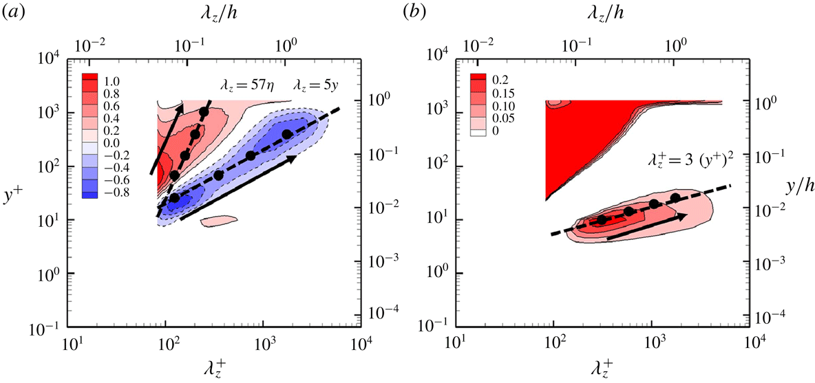
Premultiplied one-dimensional spanwise wavenumber spectra of turbulent transport
 $(Re_{\unicode[STIX]{x1D70F}}k_{z}y\widehat{T}_{turb}^{+})$
, marked with the locations to be analysed using (3.1). In (a), the dots along
 $\unicode[STIX]{x1D706}_{z}=57\unicode[STIX]{x1D702}$
are placed at
 $y_{0}^{+}=67,157,391,1033$
(
 $y_{0}/h=0.04,0.09,0.23,0.62$
), while those along
 $\unicode[STIX]{x1D706}_{z}=5y$
are at
 $y_{0}^{+}=25,67,157,391$
(
 $y_{0}/h=0.01,0.04,0.09,0.23$
). In (b), the dots along
 $\unicode[STIX]{x1D706}_{z}^{+}=3(y^{+})^{2}$
are located at
 $y_{0}^{+}=10,14,19,25$
. Note that the contour levels in (b) are adjusted to emphasize the positive values in the region close to the wall.
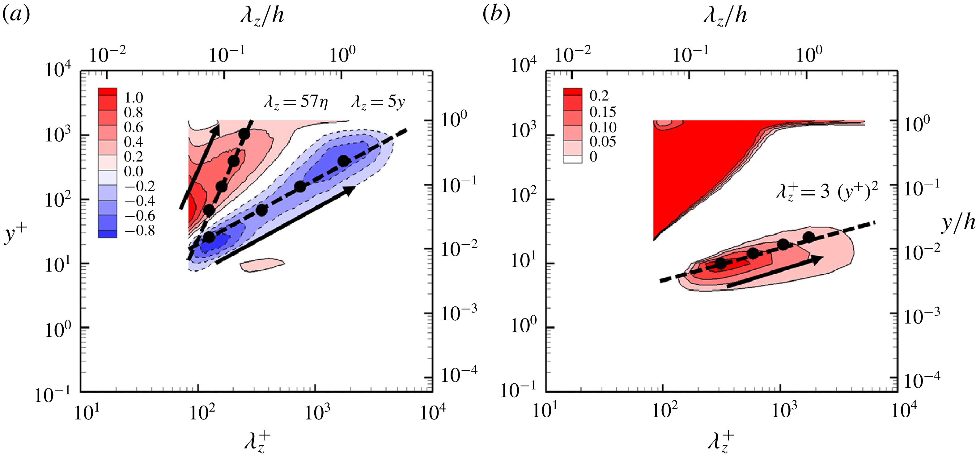
Now, we investigate the turbulent transport using the triadic interactions in (3.1) and (3.2). To avoid any unnecessary repetition of the same discussion, particular focus of our investigation is given along the three lines in figure 5: i.e.
 $\unicode[STIX]{x1D706}_{z}=57\unicode[STIX]{x1D702}$
,
 $\unicode[STIX]{x1D706}_{z}=5y$
(figure 5
a; see also figure 2
d) and
 $\unicode[STIX]{x1D706}_{z}^{+}=3(y^{+})^{2}$
(figure 5
b). The first line is placed in the middle of large positive
 $\widehat{T}_{turb}$
, and it is set to scale in the Kolmogorov microscale. Therefore, the triadic interactions associated with
 $\widehat{T}_{turb}$
along this line are expected to be the outcome of energy cascade (see also discussion below). The second line is given by
 $\unicode[STIX]{x1D706}_{z}=5y$
, and
 $\widehat{T}_{turb}$
is largely negative along this line. This line also passes through the region where TKE production is intense (figure 2
a). Finally, the third line is given by
 $\unicode[STIX]{x1D706}_{z}^{+}=3(y^{+})^{2}$
, to represent positive
 $\widehat{T}_{turb}$
in the region close to the wall (figure 5
b). In this region,
 $\widehat{T}_{turb}$
is positive, although it is weak. As already mentioned in § 3.1, we shall see that this part of the spectra plays a crucial role in the formation of the near-wall part of the TKE spectra especially at large
 $\unicode[STIX]{x1D706}_{z}$
(see also § 4.2).
Triadic interactions
 $(\widehat{T}_{turb})$
at the locations of black dots along
 $\unicode[STIX]{x1D706}_{z}=57\unicode[STIX]{x1D702}$
in figure 5(a): (a)
 $y_{0}^{+}=67$
 $(y_{0}/h=0.04)$
; (b)
 $y_{0}^{+}=157$
 $(y_{0}/h=0.09)$
; (c)
 $y_{0}^{+}=391$
 $(y_{0}/h=0.23)$
; (d)
 $y_{0}^{+}=1033$
 $(y_{0}/h=0.62)$
. Here, the black and blue dashed lines correspond to
 $l=m=k_{z,0}$
and
 $l=m=2\unicode[STIX]{x03C0}/(3y_{0})$
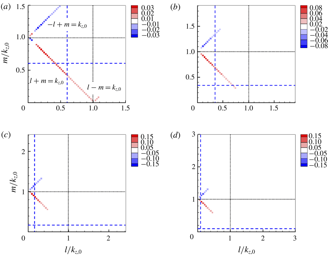
, respectively (figure 4), and the positive (red) and negative (blue) colours indicate the values of energy influx and outflux in the summation notation of (3.1), respectively.
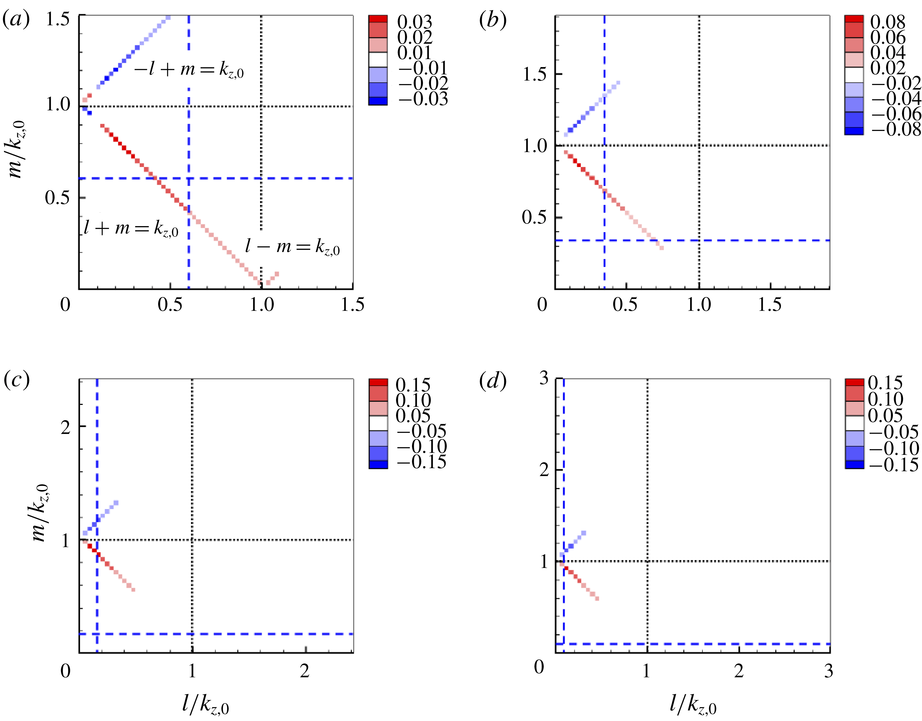
First, the triadic interactions responsible for the positive turbulent transport along
 $\unicode[STIX]{x1D706}_{z}=57\unicode[STIX]{x1D702}$
are visualized in figure 6 using (3.1) at the given wall-normal location (
 $y_{0}$
) and spanwise wavenumber (
 $k_{z,0}=2\unicode[STIX]{x03C0}/\unicode[STIX]{x1D706}_{z,0}$
). Here, positive (red) turbulent transport indicates energy influx to the given motion through interactions between eddies of wavenumber
 $l$
and
 $m$
, while negative (blue) turbulent transport represents energy outflux. The positive turbulent transport is dominated by the interactions in the region of
 $l,m<k_{z,0}$
at all the wall-normal locations considered (figure 6
a–d). This suggests that the TKE influxes to the motions scaling with
 $\unicode[STIX]{x1D706}_{z}=57\unicode[STIX]{x1D702}$
are mainly from the eddies larger than the given ones, indicating that the related turbulent transport mechanism is the energy cascade. In the near-wall region where the integral length scale (the viscous inner length scale) is identical to the Kolmogorov microscale (figure 6
a), it is difficult to identify whether the eddies involved in the positive turbulent transport are the energy-containing ones or the ones from the energy cascade due to the poor separation between the integral and dissipation length scales. However, as the wall-normal location is gradually increased, the majority of the triadic interactions for the positive turbulent transport appears in the right-upper region distinguished by the blue dashed lines (figure 6
b–d). This suggests that the positive turbulent transport along
 $\unicode[STIX]{x1D706}_{z}=57\unicode[STIX]{x1D702}$
is from the eddies in the inertial subrange, since the given motions are set to scale in the Kolmogorov microscale. Finally, it is also worth pointing out that the turbulent transport in the region of
 $l<k_{z,0}$
and
 $m>k_{z,0}$
is mostly negative at all the wall-normal locations considered. This suggests that the energy cascade is not a simple one-way forward transfer of energy from large to small scales, but an interactive process involving both forward and backward transfers of energy.
Triadic interactions
 $(\widehat{T}_{turb})$
at the locations of black dots along
 $\unicode[STIX]{x1D706}_{z}=5y$
in figure 5(a): (a)
 $y_{0}^{+}=25\;(y_{0}/h=0.01)$
; (b)
 $y_{0}^{+}=67\;(y_{0}/h=0.04)$
; (c)
 $y_{0}^{+}=157\;(y_{0}/h=0.09)$
; (d)
 $y_{0}^{+}=391\;(y_{0}/h=0.23)$
. See the caption of figure 6 for the black and blue dashed lines and for the contour label. Note that the blue dashed lines do not appear in (a) because they are located at very large
 $l$
and
 $m$
.
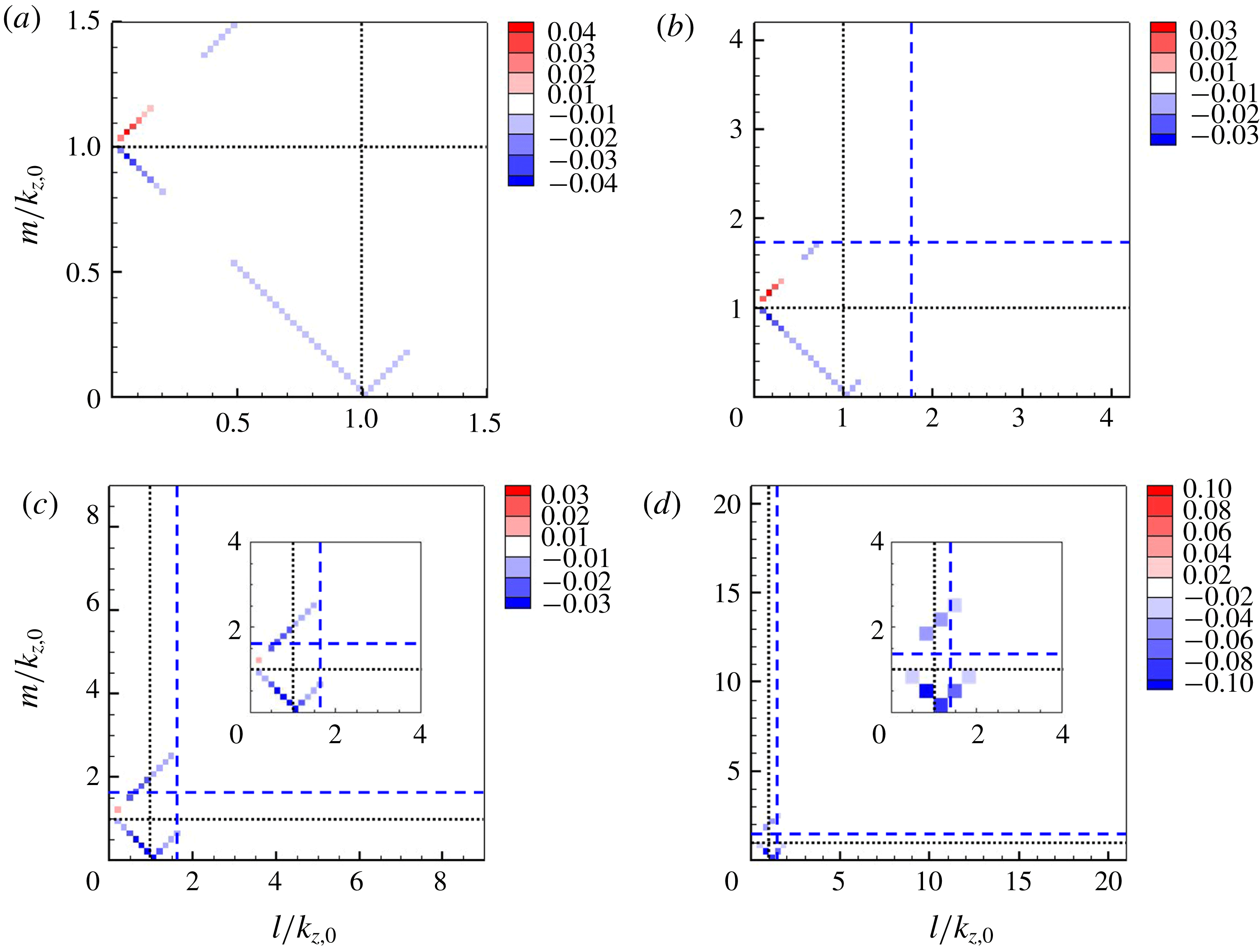
The negative turbulent transport along
 $\unicode[STIX]{x1D706}_{z}=5y$
in figure 5(a) is investigated in figure 7. In the region close to the wall (figure 7
a,b), the triadic interactions resulting in the negative turbulent transport mainly occur in the region of
 $l,m<k_{z,0}$
, indicating that the negative turbulent transport along
 $\unicode[STIX]{x1D706}_{z}=5y$
is mediated by the triad interactions between the eddies which have larger spanwise size than the given ones. Here, it is important to point out that these larger eddies participating in the negative turbulent transport are mostly the energy-containing ones, as the related triadic interactions appear mainly in the region of
 $l,m<2\unicode[STIX]{x03C0}/(3y_{0})$
. This finding therefore suggests that the interactions between large energy-containing eddies provide an important mechanism for the nonlinear turbulent transport that balances out the TKE production of smaller energy-containing eddies at the integral length scales. However, this mechanism of TKE balance at the integral length scale for such small energy-containing eddies should gradually diminish, as the wall-normal location is increased. This is because the number of the energy-containing eddies larger than the given spanwise length scale becomes reduced on increasing the wall-normal location (see figures from 7
a–d). Indeed, in the case of the highest wall-normal location considered (figure 7
d), the negative turbulent transport is generated mostly by the interactions between the eddies at similar size (i.e.
 $l,m\simeq k_{z,0}$
).
Triadic interactions
 $(\widehat{T}_{turb})$
at the locations of black dots along
 $\unicode[STIX]{x1D706}_{z}^{+}=3(y^{+})^{2}$
in figure 5(b): (a)
 $y_{0}^{+}=10$
; (b)
 $y_{0}^{+}=14$
; (c)
 $y_{0}^{+}=19$
; (d)
 $y_{0}^{+}=25$
. Here, the black dashed lines correspond to
 $l=m=k_{z,0}$
. See the caption of figure 6 for the contour label.
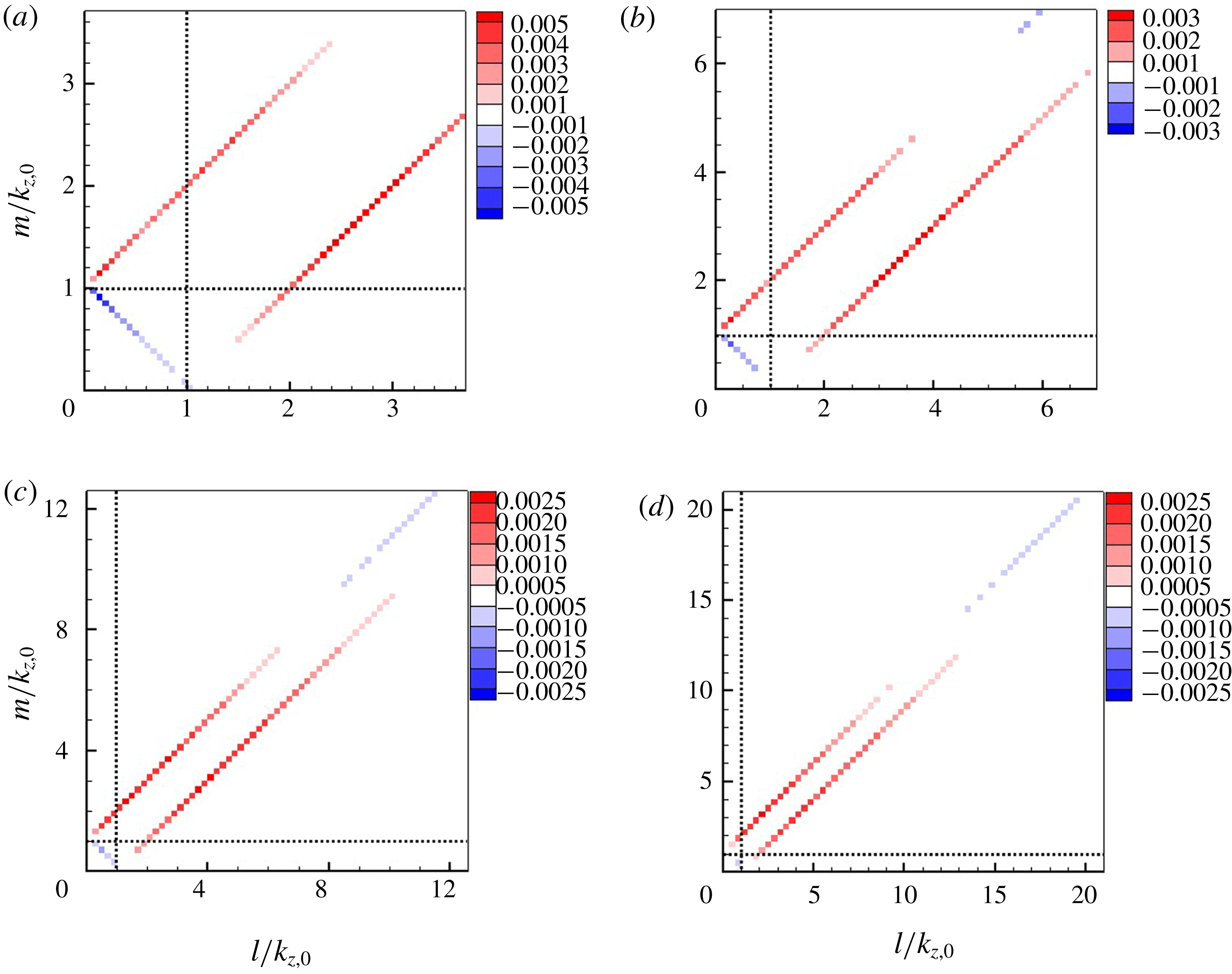
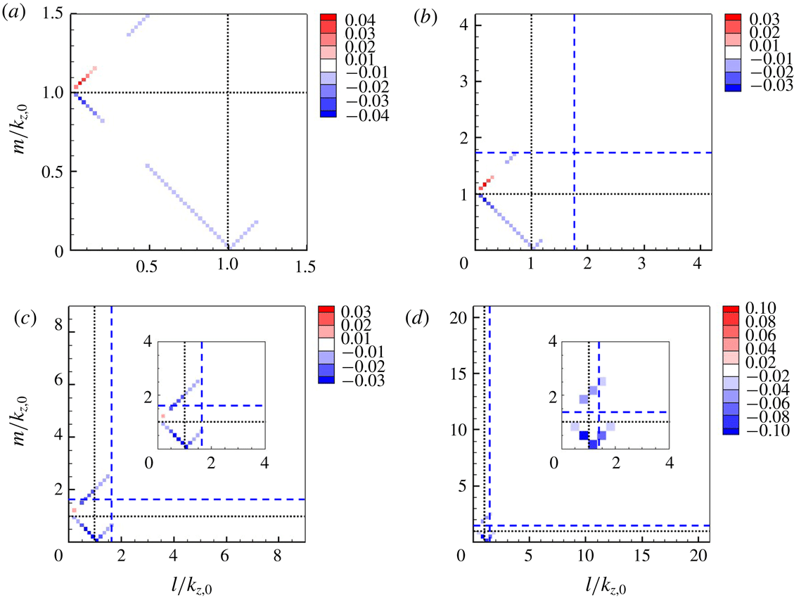
Finally, in figure 8, the origin of the weak positive turbulent transport along
 $\unicode[STIX]{x1D706}_{z}^{+}=3(y^{+})^{2}$
(figure 5
b) is explored. In this case, the majority of the related triadic interactions appear in the region of
 $l,m>k_{z,0}$
, indicating that the positive turbulent transport along
 $\unicode[STIX]{x1D706}_{z}^{+}=3(y^{+})^{2}$
is due to the interactions between the eddies, the spanwise size of which is smaller than the given ones. Furthermore, all these smaller eddies involved in the positive turbulent transport are the energy-containing ones, since all of the energetic triadic interactions emerge in the lower-left region divided by the blue-dashed lines in figure 4(b). Therefore, the positive turbulent transport along
 $\unicode[STIX]{x1D706}_{z}^{+}=3(y^{+})^{2}$
indicates the existence of positive energy transfer from small to large energy-containing eddies. However, it is important to note that the amount of the positive turbulent transport is considerably smaller than that of turbulence production at each scale (see figure 2). Therefore, disruption of this process would not significantly change the statistics in the outer region, as already demonstrated by a number of previous rough-wall experiments (e.g. Flores et al.
Reference Flores, Jiménez and del Álamo2007). In any case, the precise dynamical mechanism by which the ‘statistically’ positive turbulent transport is generated remains to be understood, and, interestingly, such an energy transfer from small to large scale was very recently observed by Kawata & Alfredsson (Reference Kawata and Alfredsson2018) in plane Couette flow at low Reynolds numbers (
 $Re_{\unicode[STIX]{x1D70F}}\leqslant 108$
). In this respect, it would be interesting to explore whether this feature has any link with the inner–outer interactions reported previously (e.g. Hutchins & Marusic Reference Hutchins and Marusic2007). Lastly, it is worth reminding that the region of
 $l,m<k_{z,0}$
in figure 8 also indicates negative turbulent transport by the interactions between larger eddies (note that this mechanism should also diminish gradually as the wall-normal location is increased), consistent with the result in figure 7.
3.3 Componentwise turbulent transport
We further investigate the TKE equation to understand the energy redistribution mechanism between individual velocity components. Each velocity component of (2.5) is written as follows:
 $$\begin{eqnarray}\displaystyle i=1:0 & = & \displaystyle \underbrace{\left\langle \text{Re}\left\{-\overline{\widehat{u^{\prime }}^{\ast }(k_{z})\widehat{v^{\prime }}(k_{z})}\,\frac{\text{d}U}{\text{d}y}\right\}\right\rangle _{x}}_{\widehat{P}(y,k_{z})}+\underbrace{\left\langle \text{Re}\left\{\overline{\widehat{p^{\prime }}(k_{z})\frac{\unicode[STIX]{x2202}\widehat{u^{\prime }}^{\ast }(k_{z})}{\unicode[STIX]{x2202}x}}\right\}\right\rangle _{x}}_{\widehat{\unicode[STIX]{x1D6F1}}_{x}(y,k_{z})}\nonumber\\ \displaystyle & & \displaystyle +\,\underbrace{\left\langle -\unicode[STIX]{x1D708}\overline{\frac{\unicode[STIX]{x2202}\widehat{u^{\prime }}(k_{z})}{\unicode[STIX]{x2202}x_{j}}\frac{\unicode[STIX]{x2202}\widehat{u^{\prime }}^{\ast }(k_{z})}{\unicode[STIX]{x2202}x_{j}}}\right\rangle _{x}}_{\widehat{\unicode[STIX]{x1D700}}_{x}(y,k_{z})}+\underbrace{\left\langle \text{Re}\left\{-\overline{\widehat{u^{\prime }}^{\ast }(k_{z})\frac{\unicode[STIX]{x2202}\widehat{\unicode[STIX]{x1D70F}_{1j}^{\prime }}(k_{z})}{\unicode[STIX]{x2202}x_{j}}}\right\}\right\rangle _{x}}_{\widehat{\unicode[STIX]{x1D700}}_{SGS,x}(y,k_{z})}\nonumber\\ \displaystyle & & \displaystyle +\,\underbrace{\left\langle \text{Re}\left\{-\overline{\widehat{u^{\prime }}^{\ast }(k_{z})\frac{\unicode[STIX]{x2202}}{\unicode[STIX]{x2202}x_{j}}\mathop{\sum }_{l+m=k_{z}}\widehat{u^{\prime }}(l)\widehat{u_{j}^{\prime }}(m)}\right\}\right\rangle _{x}}_{\widehat{T}_{turb,x}(y,k_{z})}+\underbrace{\left\langle \unicode[STIX]{x1D708}\frac{\text{d}^{2}}{\text{d}y^{2}}\left(\frac{1}{2}\overline{\left|\widehat{u^{\prime }}(k_{z})\right|^{2}}\right)\right\rangle _{x}}_{\widehat{T}_{\unicode[STIX]{x1D708},x}(y,k_{z})},\nonumber\\ \displaystyle & & \displaystyle\end{eqnarray}$$
 $$\begin{eqnarray}\displaystyle i=2:0 & = & \displaystyle \underbrace{\left\langle \text{Re}\left\{\overline{\widehat{p^{\prime }}(k_{z})\frac{\unicode[STIX]{x2202}\widehat{v^{\prime }}^{\ast }(k_{z})}{\unicode[STIX]{x2202}y}}\right\}\right\rangle _{x}}_{\widehat{\unicode[STIX]{x1D6F1}}_{y}(y,k_{z})}+\underbrace{\left\langle -\unicode[STIX]{x1D708}\overline{\frac{\unicode[STIX]{x2202}\widehat{v^{\prime }}(k_{z})}{\unicode[STIX]{x2202}x_{j}}\frac{\unicode[STIX]{x2202}\widehat{v^{\prime }}^{\ast }(k_{z})}{\unicode[STIX]{x2202}x_{j}}}\right\rangle _{x}}_{\widehat{\unicode[STIX]{x1D700}}_{y}(y,k_{z})}\nonumber\\ \displaystyle & & \displaystyle +\,\underbrace{\left\langle \text{Re}\left\{-\overline{\widehat{v^{\prime }}^{\ast }(k_{z})\frac{\unicode[STIX]{x2202}\widehat{\unicode[STIX]{x1D70F}_{2j}^{\prime }}(k_{z})}{\unicode[STIX]{x2202}x_{j}}}\right\}\right\rangle _{x}}_{\widehat{\unicode[STIX]{x1D700}}_{SGS,y}(y,k_{z})}+\underbrace{\left\langle \text{Re}\left\{-\overline{\widehat{v^{\prime }}^{\ast }(k_{z})\frac{\unicode[STIX]{x2202}}{\unicode[STIX]{x2202}x_{j}}\mathop{\sum }_{l+m=k_{z}}\widehat{v^{\prime }}(l)\widehat{u_{j}^{\prime }}(m)}\right\}\right\rangle _{x}}_{\widehat{T}_{turb,y}(y,k_{z})}\nonumber\\ \displaystyle & & \displaystyle +\,\underbrace{\left\langle \text{Re}\left\{\frac{\text{d}}{\text{d}y}\left(-\overline{\frac{\widehat{p^{\prime }}(k_{z})\widehat{v^{\prime }}^{\ast }(k_{z})}{\unicode[STIX]{x1D70C}}}\right)\right\}\right\rangle _{x}}_{\widehat{T}_{p}(y,k_{z})}+\underbrace{\left\langle \unicode[STIX]{x1D708}\frac{\text{d}^{2}}{\text{d}y^{2}}\left(\frac{1}{2}\overline{\left|\widehat{v^{\prime }}(k_{z})\right|^{2}}\right)\right\rangle _{x}}_{\widehat{T}_{\unicode[STIX]{x1D708},y}(y,k_{z})},\end{eqnarray}$$
 $$\begin{eqnarray}\displaystyle i=3:0 & = & \displaystyle \underbrace{\left\langle \text{Re}\left\{\overline{\widehat{p^{\prime }}(k_{z})\left(\text{i}k_{z}\widehat{w^{\prime }}(k_{z})\right)^{\ast }}\right\}\right\rangle _{x}}_{\widehat{\unicode[STIX]{x1D6F1}}_{z}(y,k_{z})}+\underbrace{\left\langle -\unicode[STIX]{x1D708}\overline{\frac{\unicode[STIX]{x2202}\widehat{w^{\prime }}(k_{z})}{\unicode[STIX]{x2202}x_{j}}\frac{\unicode[STIX]{x2202}\widehat{w^{\prime }}^{\ast }(k_{z})}{\unicode[STIX]{x2202}x_{j}}}\right\rangle _{x}}_{\widehat{\unicode[STIX]{x1D700}}_{z}(y,k_{z})}\nonumber\\ \displaystyle & & \displaystyle +\,\underbrace{\left\langle \text{Re}\left\{-\overline{\widehat{w^{\prime }}^{\ast }(k_{z})\frac{\unicode[STIX]{x2202}\widehat{\unicode[STIX]{x1D70F}_{3j}^{\prime }}(k_{z})}{\unicode[STIX]{x2202}x_{j}}}\right\}\right\rangle _{x}}_{\widehat{\unicode[STIX]{x1D700}}_{SGS,z}(y,k_{z})}+\underbrace{\left\langle \text{Re}\left\{-\overline{\widehat{w^{\prime }}^{\ast }(k_{z})\frac{\unicode[STIX]{x2202}}{\unicode[STIX]{x2202}x_{j}}\mathop{\sum }_{l+m=k_{z}}\widehat{w^{\prime }}(l)\widehat{u_{j}^{\prime }}(m)}\right\}\right\rangle _{x}}_{\widehat{T}_{turb,z}(y,k_{z})}\nonumber\\ \displaystyle & & \displaystyle +\,\underbrace{\left\langle \unicode[STIX]{x1D708}\frac{\text{d}^{2}}{\text{d}y^{2}}\left(\frac{1}{2}\overline{\left|\widehat{w^{\prime }}(k_{z})\right|^{2}}\right)\right\rangle _{x}}_{\widehat{T}_{\unicode[STIX]{x1D708},z}(y,k_{z})},\end{eqnarray}$$
 $\widehat{\unicode[STIX]{x1D6F1}}_{x},\widehat{\unicode[STIX]{x1D6F1}}_{y}$
and
 $\widehat{\unicode[STIX]{x1D6F1}}_{z}$
are the spanwise wavenumber spectra of the streamwise, wall-normal and spanwise components of pressure–strain terms, respectively. We note that the pressure–strain terms do not appear in (2.5) because the continuity leads to
 $$\begin{eqnarray}\widehat{\unicode[STIX]{x1D6F1}}_{x}(y,k_{z})+\widehat{\unicode[STIX]{x1D6F1}}_{y}(y,k_{z})+\widehat{\unicode[STIX]{x1D6F1}}_{z}(y,k_{z})=0.\end{eqnarray}$$
This relation also indicates that the pressure–strain terms play a central role in the TKE distribution to the individual velocity components. Equation (3.4) evidently suggests that the turbulence production appears only in (3.4a
) and there is no such terms in (3.4b
) and (3.4c
). Therefore, the pressure terms
 $\widehat{\unicode[STIX]{x1D6F1}}_{y}$
and
 $\widehat{\unicode[STIX]{x1D6F1}}_{z}$
should act as the driving terms in (3.4b
) and (3.4c
), respectively, and this is the only possible way to distribute the TKE produced at the streamwise component to the other components.
Premultiplied one-dimensional spanwise wavenumber spectra of pressure–strain: (a)
 $\widehat{\unicode[STIX]{x1D6F1}}_{x}(y,k_{z})$
; (b)
 $\widehat{\unicode[STIX]{x1D6F1}}_{y}(y,k_{z})$
; (c)
 $\widehat{\unicode[STIX]{x1D6F1}}_{z}(y,k_{z})$
.
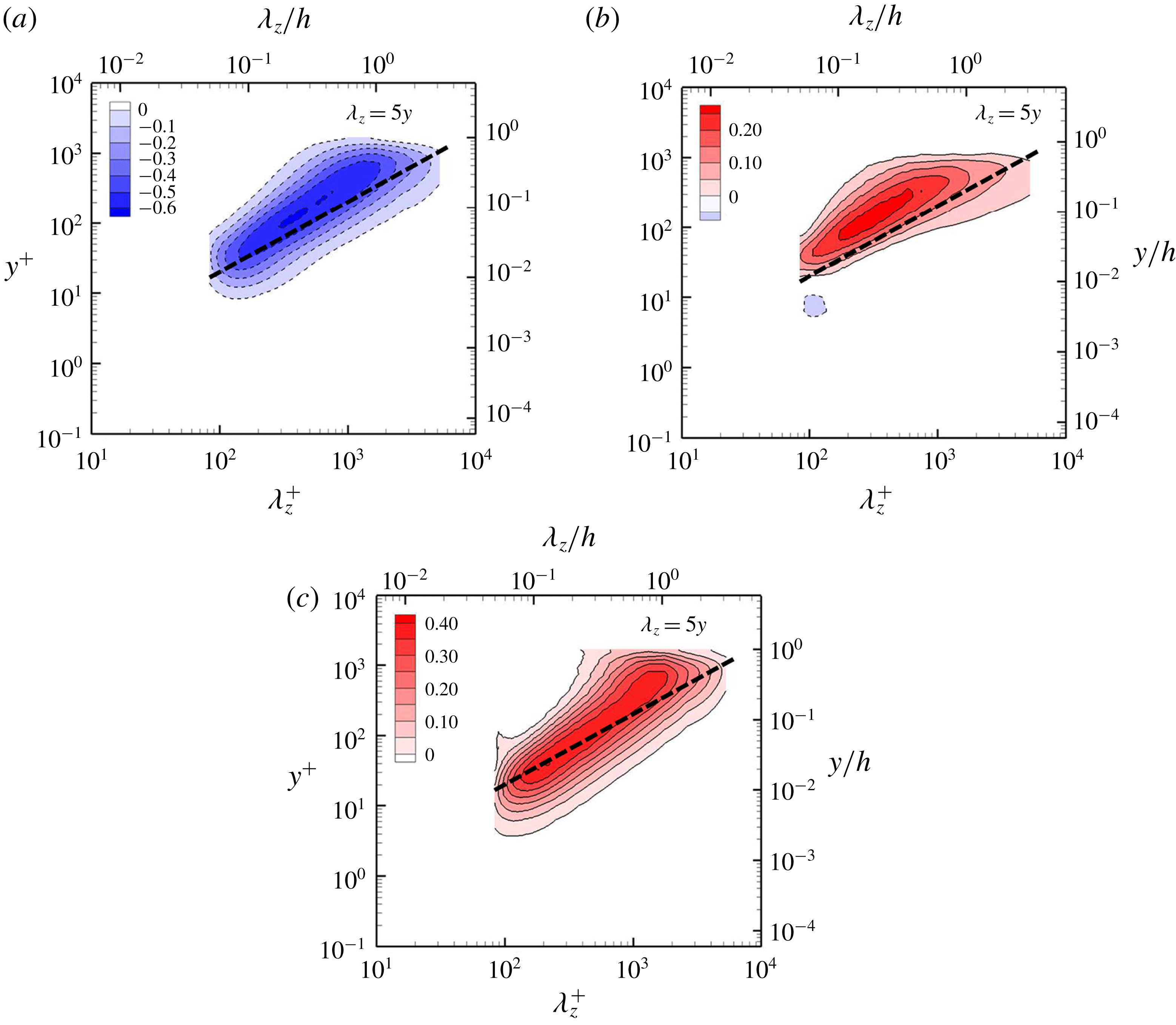
Since the pressure–strain spectra and their scaling behaviour with the Reynolds number have recently been discussed in detail by Lee & Moser (Reference Lee and Moser2015a
) and Mizuno (Reference Mizuno2016), here we only briefly report the pressure–strain spectra in figure 9. As expected, the pressure–strain spectra for the streamwise component of TKE are negative, confirming its role of transferring TKE to the other velocity components (figure 9
a). The pressure–strain spectra for the wall-normal and spanwise velocity components are positive almost everywhere in the
 $\unicode[STIX]{x1D706}_{z}$
–
 $y$
plane, except in the near-wall region where the spectra for the wall-normal component are slightly negative. This tendency of the present LES is consistent with that of the DNS data (Hoyas & Jiménez Reference Hoyas and Jiménez2008; Mizuno Reference Mizuno2016). Here, we only stress that all the pressure–strain spectra are well aligned with
 $\unicode[STIX]{x1D706}_{z}=5y$
, implying that the energy distribution process to each component takes place at the integral length scale. We will discuss this issue later in § 4.3.
Premultiplied one-dimensional spanwise wavenumber spectra of the (a) streamwise, (b) wall-normal and (c) spanwise components of turbulent transport.
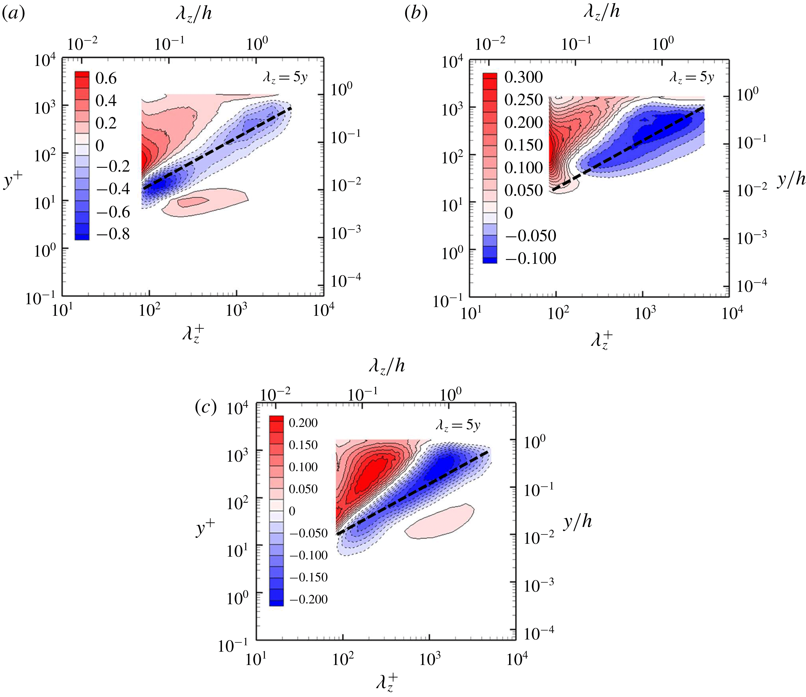
Figure 10 shows turbulent transport spectra for each component of the TKE. Similarly to the turbulent transport spectra for the total TKE (figure 2
d), all the spectra reveal the typical feature associated energy cascade: the negative parts of the spectra are approximately aligned along
 $\unicode[STIX]{x1D706}_{z}=5y$
, while the positive parts appear in the region where energy cascade and dissipation are relevant. However, it is important to note that the weak positive parts in the spectra appear only for the streamwise and spanwise components, whereas the spectra for the wall-normal component do not exhibit such a behaviour. This observation reminds us of the statistical structure of the individual energy-containing motions (i.e. attached eddies) hypothesized by Townsend (Reference Townsend1976) – only their streamwise and spanwise components contain the wall-reaching part, which is inactive in the sense that they do not carry any Reynolds shear stress. In this respect, this also suggests that the weak positive part in the near-wall turbulent transport spectra would probably be related to the formation of the wall-reaching part of the streamwise and spanwise components of the energy-containing eddies. In § 4.2, we shall indeed see that it plays a crucial role in the formation of the wall-reaching part of the energy-containing motions in the log and outer regions. Finally, it is worth noting that the spanwise component of the near-wall positive turbulent transport spectra appears further away from the wall than the streamwise one. This feature is difficult to provide a satisfactory explanation solely with the present statistical analysis, as it would require a detailed knowledge of the related fluid motions. However, the spanwise component of energy-containing eddies has been associated with the self-similar vortical structures statistically in the form of quasi-streamwise vortices (Hwang Reference Hwang2015). These structures tend to appear to be located a little further away from the wall than the streaky motions at the same spanwise length scale (Hwang Reference Hwang2015), and this might be related to different wall-normal locations of the positive turbulent transport spectra for the streamwise and spanwise components.
4 Discussion
Thus far, we have explored the detailed processes of spectral energy transfer and scale interactions using the spanwise spectral TKE equation (2.5). Turbulence production is almost uniform over the entire integral scale, especially in the log region (figure 2
a), and it originates from the linear part of the Navier–Stokes equation. The transfer of the produced TKE and the related scale interactions are investigated by analysing the triadic interaction form of turbulent transport
 $\widehat{T}_{turb}(y,k_{z})$
. The major role played by the turbulent transport is the energy cascade down to the Kolmogorov microscale, as in many other turbulent shear flows. Further to this, in the present study, two new types of scale interactions have been discovered. First, for relatively small energy-containing motions, part of the energy transfer mechanisms from the integral to the adjacent length scale in the energy cascade is found to be provided by interactions between larger energy-containing motions (figure 7). Second, there exists a non-negligible amount of energy transfer from small to large scales (figure 8), and this is particularly important for the streamwise and spanwise velocity components in the near-wall region (figure 10
a,c). It is finally worth noting that both of the scale interaction processes found in the present study are highly active in the near-wall region where all the energy-containing motions would reach to some extent.
4.1 Energy cascade and dissipation of small energy-containing motions
The production (figure 2
a) and turbulent transport (figure 2
d) spectra suggest that, at the integral length scales (i.e.
 $\unicode[STIX]{x1D706}_{z}\sim 5y$
), turbulence production in the log and outer regions is mainly balanced with nonlinear turbulent transport (negative (blue) region in figure 2
d). This is a natural consequence of small dissipation at such large length scales because dissipation is inversely proportional to the square of given length scale. In the region close to the wall where the integral length scale is relatively small (i.e. the near-wall region and lower part of the log layer), we have seen that a significant amount of the negative turbulent transport is provided by the interactions between the energy-containing motions at larger integral length scales (figure 7). This implies that part of the energy cascade mechanisms for the energy-containing motions in this region is associated with the presence of larger energy-containing motions. It is yet to be understood what kind of dynamical processes of such large energy-containing motions are precisely responsible for this. However, it should be noted that this observation appears to be linked to previous studies by Hwang (Reference Hwang2013) and de Giovanetti et al. (Reference de Giovanetti, Hwang and Choi2016), who have shown appreciable contribution of large energy-containing motions to skin-friction generation by artificially removing them.
We imagine a situation where some of relatively large energy-containing motions are artificially removed by an external means (e.g. control, artificial damping, confinement of the domain size, etc.). From the triadic interaction analysis in figure 7, the small energy-containing motions in the region close to the wall are expected to lose some of the energy transfer mechanisms to the adjacent smaller length scale in the energy cascade process. Then, one may expect that the reduced turbulent transport would not fully remove the original turbulence production, seemingly breaking the TKE balance at the integral length scales. However, it should be remembered that the removal of such large energy-containing motions also leads to reduction of skin friction, thereby reducing the corresponding friction velocity. Therefore, in such a circumstance, the turbulence production for the small energy-containing motions would also be reduced because turbulence production is proportional to the cube of the friction velocity: i.e.
 $P(y)\simeq u_{\unicode[STIX]{x1D70F}}^{3}/(\unicode[STIX]{x1D705}y)$
. In this respect, the loss of turbulent transport mechanism by the removal of large energy-containing motions does not necessarily imply the broken TKE balance at small integral length scales in the region close to the wall, because the reduced negative turbulent transport could be equalized by the reduced turbulence production.
However, it is also worth mentioning that the same scenario would not hold in the near-wall region where the smallest inner-scaling energy-containing motions reside. In this region, there is very little separation between the integral and dissipation length scales, indicating that the related turbulence production is directly balanced with dissipation without having energy cascade. Therefore, the removal of large energy-containing motions would simply cause an excess of dissipation at the given integral length scale because the turbulence production would be weakened by the reduced friction velocity. In this case, the energy-containing motions at the original smallest integral length scale would not be sustained anymore because the dissipation at this length scale is expected to be greater than the reduced production. Consequently, the new smallest energy-containing motions would be formed at a larger length scale where the reduced turbulence production would be balanced with dissipation. If the near-wall motions are assumed to be universal, the expected spanwise length scale of the new smallest energy-containing motions would be
 $\unicode[STIX]{x1D706}_{z}^{+}\simeq 100$
based on the reduced friction velocity. This is consistent with our recent observations (Hwang Reference Hwang2013; de Giovanetti et al.
Reference de Giovanetti, Hwang and Choi2016), where the removal of large energy-containing motions was shown not to change the inner-scaled spectra in the near-wall region.
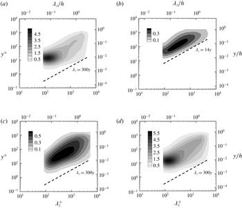
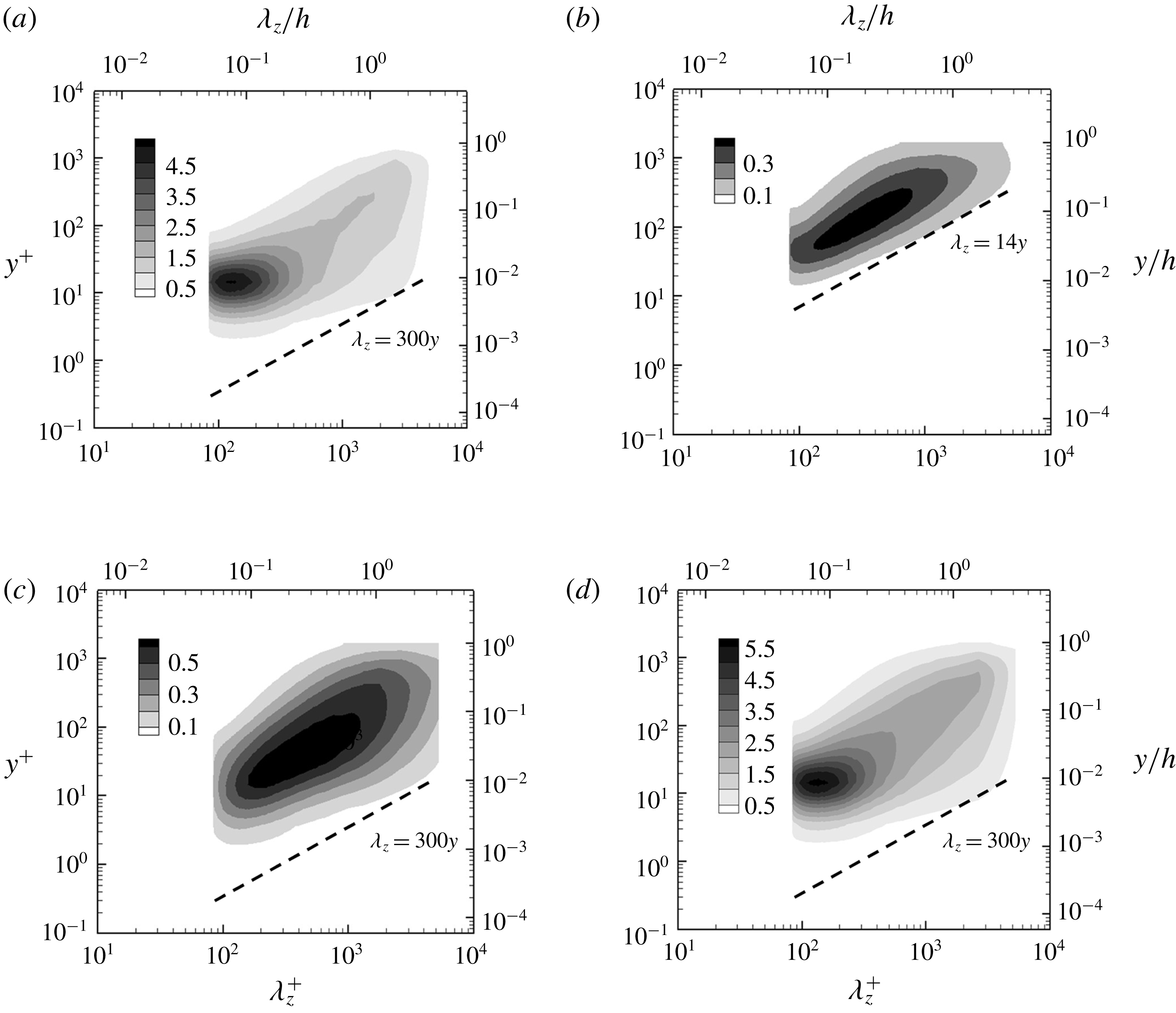
Premultiplied one-dimensional spanwise wavenumber spectra of (a) streamwise, (b) wall-normal, (c) spanwise velocities and (d) turbulent kinetic energy.
Finally, it is worth mentioning that the discussion given here places an emphasis on the relevance of turbulence control targeting relatively large energy-containing motions, since their removal or suppression would automatically reduce turbulence production of the near-wall energy-containing motions as well. However, to our knowledge, such flow control strategies resulting in any appreciable amount of turbulent drag reduction (say
 $20\,\%$
) are not available yet, and their development remains an important task to be achieved in the near future.
4.2 Positive near-wall turbulent transport and the formation of inactive motion
Penetration of the energy-containing motions of the log and outer regions into the near-wall region has been repeatedly reported by a number of recent studies (e.g. Hutchins & Marusic Reference Hutchins and Marusic2007; Mathis et al. Reference Mathis, Hutchins and Marusic2009). This feature was also described in the attached eddy hypothesis (Townsend Reference Townsend1976), where each of the energy-containing motions in the log and outer regions is modelled to reach the near-wall region through their streamwise and spanwise components. In the original theory of Townsend (Reference Townsend1976), this is the key statistical feature of each attached eddy, as it is the mathematical origin of the logarithmic wall-normal dependence of the streamwise and spanwise turbulence intensities. He also pointed out that the wall-reaching part of each attached eddy would be ‘inactive’ in the sense that it does not carry any Reynolds shear stress, and this is the natural consequence of the fact that the wall-normal component of the attached eddy cannot be large in the near-wall region due to the boundary condition at the wall.
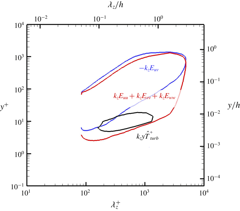
Overlapped premultiplied one-dimensional spanwise wavenumber spectra of turbulent kinetic energy (red), Reynolds shear stress (blue) and the near-wall positive turbulent transport (black). Here, the contour lines for both turbulent kinetic energy and Reynolds shear stress indicate 15 % of their respective maxima, while that of turbulent transport indicates 10 % of the maximum.

The inactive wall-reaching part of the energy-containing motions can also be found by examining the premultiplied one-dimensional spanwise wavenumber spectra of each velocity component. In figure 11, it is seen that the spectra of the streamwise and spanwise velocities exhibit a non-negligible amount of energy in the region close to the wall (figure 11
a,c), and this part of the spectra does not precisely follow any linear scaling in that region. To clearly show this, a dashed line (
 $\unicode[STIX]{x1D706}_{z}\simeq 300y$
) is drawn at the lower part of the spectra. On the other hand, the spectra of the wall-normal velocity do not show any substantial amount of energy in the near-wall region, and the lower part of the spectra follows a linear scaling fairly well (
 $\unicode[STIX]{x1D706}_{z}\simeq 14y$
in figure 11
b). The spectra of the TKE are fairly similar to those of the streamwise velocity because the TKE is dominated by the streamwise component (figure 11
d). For the same reason, the spectra of the TKE also reveal an appreciable amount of energy in the near-wall region, and do not follow any linear scaling in that region (figure 11
d). Finally, it should be mentioned that exactly the same feature appears in the streamwise wavenumber spectra, as recently shown by Hwang (Reference Hwang2016).
In figure 12, the spectra of the TKE, the Reynolds shear stress and the near-wall positive turbulent transport are plotted together. This figure now confirms that the wall-reaching part of the energy-containing motions at large
 $\unicode[STIX]{x1D706}_{z}$
carries little Reynolds shear stress. As discussed with figure 11, this part of the TKE spectra is mainly contributed by the streamwise and spanwise components, thereby consistently representing the wall-reaching inactive part of each attached eddy (Townsend Reference Townsend1976). It should be mentioned that the Reynolds shear-stress spectra in figure 12 should be very similar to those of turbulence production because
 $k_{z}y\widehat{P}(y,k_{z})=-k_{z}yE_{uv}(y,k_{z})\,\text{d}U/\text{d}y$
(
 $E_{uv}(y,k_{z})$
is the spectrum of Reynolds shear stress) and
 $\text{d}U/\text{d}y\sim 1/y$
. Therefore, it would be difficult to imagine that the near-wall inactive part of the TKE spectra is a direct outcome of turbulence production. In this respect, it is important to note that this part of the TKE spectra significantly overlaps with the near-wall positive turbulent transport, indicating that the main driving mechanism of the inactive part of the motion is likely to be the positive turbulent transport in the region close to the wall.
If the positive turbulent transport becomes the driving mechanism of the near-wall part of large energy-containing motion, it is evident that the classical energy cascade is not the way to form the TKE balance in the near-wall region at large
 $\unicode[STIX]{x1D706}_{z}$
– indeed, the positive turbulent transport in the near-wall region has been shown to be the consequence of energy transfer from smaller energy-containing eddies (figure 8). To gain further physical insight into the mechanism of the near-wall TKE balance at such a large length scale, the wall-normal profiles of the terms on the right-hand side of (2.5) for
 $\unicode[STIX]{x1D706}_{z}=0.5h$
and
 $1.5h$
are examined in figure 13. Here, we note that the vertical dashed lines correspond to the wall-normal location given by
 $\unicode[STIX]{x1D706}_{z}^{+}=3(y^{+})^{2}$
(figure 5) and that the dissipation term is the sum of the viscous and SGS dissipations. It turns out that the main TKE balance at large
 $\unicode[STIX]{x1D706}_{z}$
(small
 $k_{z}$
) in the near-wall region (
 $y^{+}\lesssim 20$
) is formed between the positive turbulent transport and dissipation, and this is more apparent for larger spanwise wavelength (figure 13
b). Assuming that the SGS dissipation is negligible in a fully resolved simulation such as a DNS, the approximate TKE balance in the near-wall region for large
 $\unicode[STIX]{x1D706}_{z}$
is therefore given by
 $$\begin{eqnarray}\widehat{T}_{turb}(y,k_{z})\simeq \left\langle -\unicode[STIX]{x1D708}\overline{\frac{\unicode[STIX]{x2202}\widehat{u_{i}^{\prime }}(y,k_{z})}{\unicode[STIX]{x2202}x_{j}}\frac{\unicode[STIX]{x2202}\widehat{u_{i}^{\prime }}^{\ast }(y,k_{z})}{\unicode[STIX]{x2202}x_{j}}}\right\rangle _{x}.\end{eqnarray}$$
Wall-normal profiles of the terms on the right-hand side of (2.5) for (a)
 $\unicode[STIX]{x1D706}_{z}=0.5h$
and (b)
 $\unicode[STIX]{x1D706}_{z}=1.5h$
: ——, (red), production; ——, (blue), sum of viscous and SGS dissipations; ——, (black), turbulent transport; –
 $\cdot$
–, pressure transport; – – –, viscous transport. Here, the vertical dashed lines indicate the wall-normal location given by
 $\unicode[STIX]{x1D706}_{z}^{+}=3(y^{+})^{2}$
(figure 5).

Now, let us recall the form of turbulent transport
 $\widehat{T}_{turb}(y,k_{z})$
in (2.5). Due to the large
 $\unicode[STIX]{x1D706}_{z}$
of interest (i.e.
 $\unicode[STIX]{x1D706}_{z}\gg y$
),
 $\unicode[STIX]{x2202}/\unicode[STIX]{x2202}x_{j}\sim \unicode[STIX]{x2202}/\unicode[STIX]{x2202}y$
and
 $\widehat{u_{i}^{\prime }u_{j}^{\prime }}\sim \widehat{u_{i}^{\prime }v^{\prime }}$
. Here, we note that, given
 $\widehat{T}_{turb}(y,k_{z})$
in the form of (3.1),
 $\widehat{u_{i}^{\prime }v^{\prime }}$
becomes the non-zero driving term stemming mostly from the other wavenumbers (see also (4.7) for a further discussion). In particular, it includes
 $\widehat{u^{\prime }v^{\prime }}$
and
 $\widehat{v^{\prime }v^{\prime }}$
. These two terms resemble the Reynolds stress components that scale very well with the inner units in the near-wall region, due to the presence of
 $v^{\prime }$
(see also the DNS data in Lee & Moser Reference Lee and Moser2015b
). From this observation, we assume
 $\widehat{u_{i}^{\prime }v^{\prime }}\sim u_{\unicode[STIX]{x1D70F}}^{2}$
. Then, the magnitude of the left-hand side of (4.1) would be given at
 $O(\widehat{u_{i}^{\prime }}(y,k_{z})u_{\unicode[STIX]{x1D70F}}^{2}/y)$
. Similarly, that of the right-hand side is given at
 $O(\unicode[STIX]{x1D708}(\widehat{u_{i}^{\prime }}(y,k_{z})/y)^{2})$
. The order of magnitude balance in (4.1) subsequently leads to
 $$\begin{eqnarray}\widehat{u_{i}^{\prime }}(y,k_{z})\frac{u_{\unicode[STIX]{x1D70F}}^{2}}{y}\sim \unicode[STIX]{x1D708}\left(\frac{\widehat{u_{i}^{\prime }}(y,k_{z})}{y}\right)^{2},\end{eqnarray}$$
where
 $y$
indicates the wall-normal location of the wall-reaching inactive part of the given large energy-containing motion, the spanwise wavenumber of which is given by
 $k_{z}(\equiv 2\unicode[STIX]{x03C0}/\unicode[STIX]{x1D706}_{z})$
. Then, (4.2) yields the strength of the inactive part in the region close to the wall, such that:
 $$\begin{eqnarray}\frac{\widehat{u_{i}^{\prime }}(y,k_{z})}{u_{\unicode[STIX]{x1D70F}}}\sim y^{+},\end{eqnarray}$$
or, equivalently,
 $$\begin{eqnarray}\frac{\widehat{u_{i}^{\prime }}(y,k_{z})}{u_{\unicode[STIX]{x1D70F}}}\sim Re_{\unicode[STIX]{x1D70F}}\frac{y}{h}.\end{eqnarray}$$
Here, it is important to note that the scaling (4.3) is strictly valid for
 $\unicode[STIX]{x1D706}_{z}\gg y$
. This is also the reason why the strength of the inactive motion
 $\widehat{u_{i}^{\prime }}(y,k_{z})/u_{\unicode[STIX]{x1D70F}}$
becomes only a function of
 $y$
.
The order of magnitude balance (4.2) and its consequence (4.3) provide some important physical insight into the scaling of inactive motions and the associated dissipation. First, (4.3) suggests that the wall-normal profile of large energy-containing motions in the near-wall region should scale in the inner unit as long as
 $\unicode[STIX]{x1D706}_{z}\gg y$
. This is consistent with the observation by Hwang (Reference Hwang2016), who showed that the wall-reaching inactive part of large energy-containing motions scales in the inner unit. He further explained that this is also the essential reason why the wall-normal location of the so-called outer peak in the streamwise wavenumber spectra of streamwise velocity becomes a function of
 $Re_{\unicode[STIX]{x1D70F}}$
(for detailed discussion, see Hwang Reference Hwang2016). Second, (4.3) is only valid for the streamwise and spanwise components of the motion (i.e.
 $i=1,3$
). This is because the left- and right-hand sides of (4.2) are proportional to
 $\widehat{u_{i}^{\prime }}(y,k_{z})$
and
 $(\widehat{u_{i}^{\prime }}(y,k_{z}))^{2}$
. If
 $i=2$
, the impermeability condition for the wall-normal velocity makes both left- and right-hand sides of (4.2) become zero at the leading order in the region close to the wall. Finally, (4.2) and (4.3) indicate that dissipation at large
 $\unicode[STIX]{x1D706}_{z}$
is given by
 $$\begin{eqnarray}\widehat{\unicode[STIX]{x1D716}}(y,k_{z})\sim \frac{u_{\unicode[STIX]{x1D70F}}^{4}}{\unicode[STIX]{x1D708}},\end{eqnarray}$$
which still scales in the inner units. However, this does not necessarily imply that the inner-scaled near-wall dissipation
 $\unicode[STIX]{x1D716}^{+}(y)$
is not a function of
 $Re_{\unicode[STIX]{x1D70F}}$
. The inner-scaled dissipation is given by
 $$\begin{eqnarray}\unicode[STIX]{x1D716}^{+}(y)=2\int _{0}^{\infty }\widehat{\unicode[STIX]{x1D716}}^{+}(y,k_{z})\,\text{d}k_{z}^{+}=2\int _{k_{z,l}^{+}Re_{\unicode[STIX]{x1D70F}}}^{k_{z,u}^{+}}\widehat{\unicode[STIX]{x1D716}}^{+}(y,k_{z})\,\text{d}k_{z}^{+},\end{eqnarray}$$
where
 $k_{z,l}^{+}Re_{\unicode[STIX]{x1D70F}}$
and
 $k_{z,u}^{+}$
are the lower and upper bounds of the compact support of
 $\widehat{\unicode[STIX]{x1D716}}^{+}(y,k_{z})$
in the inner unit, respectively, Here, we note that the lower bound is given by
 $k_{z,l}^{+}Re_{\unicode[STIX]{x1D70F}}$
as it should scale in the outer unit. Therefore, (4.5) indicates that
 $\unicode[STIX]{x1D716}^{+}(y)$
in the near-wall region would have a dependency on the Reynolds number, even if
 $\widehat{\unicode[STIX]{x1D716}}(y,k_{z})$
scales in the inner unit, and this is consistent with its behaviour reported by Hoyas & Jiménez (Reference Hoyas and Jiménez2008). It has been speculated that this behaviour is due to the inactive part of large energy-containing motions in the near-wall region (Bradshaw Reference Bradshaw1967; Hoyas & Jiménez Reference Hoyas and Jiménez2008), and the present analysis provides direct support of this idea.
The analysis above evidently suggests the crucial role played by the positive turbulent transport in the formation and scaling of the inactive part of large energy-containing motions in the near-wall region. We note that the positive turbulent transport in the near-wall region should originate from the log and outer regions, as the following quantity representing the wall-normal advective TKE flux (see (2.5) and (2.6)) is negative for sufficiently small
 $y$
and large
 $\unicode[STIX]{x1D706}_{z}$
(see also Mizuno Reference Mizuno2016):
 $$\begin{eqnarray}\widehat{\unicode[STIX]{x1D6E9}}_{turb}(y,k_{z})=-\int _{0}^{y}\widehat{T}_{turb}(y,k_{z})\,\text{d}y.\end{eqnarray}$$
This feature is seemingly consistent with the recent linear analysis by Hwang (Reference Hwang2016), who proposed that the downward TKE transport into the near-wall region is the feature recovered by a simple mixing length model based on inhomogeneous eddy viscosity in the wall-normal direction. In that model, the formation of the wall-reaching inactive motion was described by diffusive transport of TKE, and this process takes place only within the considered
 $\unicode[STIX]{x1D706}_{z}$
because of the linear nature of the model that does not allow for any energy transfer across different length scales. However, the triadic interaction analysis in the present study suggests that the actual mechanism of the downward turbulent transport into the near-wall region is much more complicated than that described by the simple mixing length model.
To demonstrate this, let us first set
 $l=k_{z}(\equiv 2\unicode[STIX]{x03C0}/\unicode[STIX]{x1D706}_{z})$
and
 $m=0$
in the convolution of (3.1). The turbulent transport can then be rearranged to yield the wall-normal derivative of the downward TKE flux within the given
 $\unicode[STIX]{x1D706}_{z}$
, such that:
 $$\begin{eqnarray}\widehat{T}_{turb}(y,k_{z})=\left\langle \text{Re}\left\{-\overline{\frac{\unicode[STIX]{x2202}}{\unicode[STIX]{x2202}y}(\widehat{e}(k_{z})\widehat{v^{\prime }}(0))}\right\}\right\rangle _{x},\end{eqnarray}$$
where
 $\widehat{v^{\prime }}(0)$
is the spatial average of the wall-normal velocity in the homogeneous directions. Therefore, for infinitely large computational domain,
 $\widehat{v^{\prime }}(0)=0$
, indicating that the downward turbulent transport within the given
 $\unicode[STIX]{x1D706}_{z}$
should be zero. Indeed, in figure 8, the values of
 $\widehat{T}_{turb}$
around
 $l=k_{z}$
and
 $m=0$
are either close to zero or very small. This suggests that the positive turbulent transport in the near-wall region cannot originate from the energy-containing motions at the same spanwise length scale. Instead, it is primarily from the interactions between the energy-containing motions, the spanwise size of which is smaller than the given
 $\unicode[STIX]{x1D706}_{z}$
(figure 8). It is important to point out that this conclusion is also consistent with the observation by Mizuno (Reference Mizuno2016), who showed that the positive turbulent transport in the near-wall region at large
 $\unicode[STIX]{x1D706}_{z}$
becomes enhanced with an increase of the Reynolds number (figure 3b in Mizuno Reference Mizuno2016): for
 $\unicode[STIX]{x1D706}_{z}$
chosen to scale in the outer unit (e.g.
 $\unicode[STIX]{x1D706}_{z}=1h$
), the increase of the Reynolds number should increase the number of smaller energy-containing motions, thereby elevating the value of the near-wall positive turbulent transport at the given
 $\unicode[STIX]{x1D706}_{z}$
. This also suggests that the wall-reaching inactive part of energy-containing motions in the log and outer regions would be developed more on increasing the Reynolds number, as also shown with (4.3b
).
4.3 Pressure–strain spectra and self-sustaining process
An important limitation of the present analysis is that it does not connect to ‘dynamical features’ of fluid motions. Indeed, it only analyses statistical features in the energetics, and it does not provide any information about how such energetics is linked to the actual motions of eddies. However, there are some interesting features that can be discussed in terms of self-sustaining process of energy-carrying eddies (Hwang Reference Hwang2015; Hwang & Bengana Reference Hwang and Bengana2016), and the pressure–strain spectra (figure 9) provide particularly useful information in this regard. It has been found that all the pressure–strain spectra are well aligned with
 $\unicode[STIX]{x1D706}_{z}=5y$
, consistent with the attached eddy hypothesis. This indicates that the TKE distribution process takes place at each integral length scale, which support the so-called self-sustaining process for all the energy-containing motions in the form of Townsend’s attached eddies (Hwang Reference Hwang2015; Hwang & Bengana Reference Hwang and Bengana2016). As discussed in § 2.1, turbulence production can be viewed as a scale-independent process in the sense that it originates from the linearized Navier–Stokes equation. In the absence of any inflection point in the mean shear, the turbulence production should involve the lift-up effect, as they share the same mathematical origin in (2.1). The lift-up effect has been firmly understood as the amplification mechanism of streaky motions. However, this amplification mechanism is only active in the presence of the driving nonlinearity (i.e. second term in (2.1b
)) due to the marginally stable or stable nature of the linearized Navier–Stokes equation around the mean flow (Malkus Reference Malkus1956; Pujals et al.
Reference Pujals, García-Villalba, Cossu and Depardon2009). In particular, the driving nonlinearity should be able to excite the wall-normal velocity fluctuation
 $v^{\prime }$
for the generation of such streaky motions, given the wall-normal velocity and vorticity form of the linearized Navier–Stokes equation (for a detailed discussion, see also de Giovanetti, Sung & Hwang Reference de Giovanetti, Sung and Hwang2017).
Energy distribution mechanism via self-sustaining process.
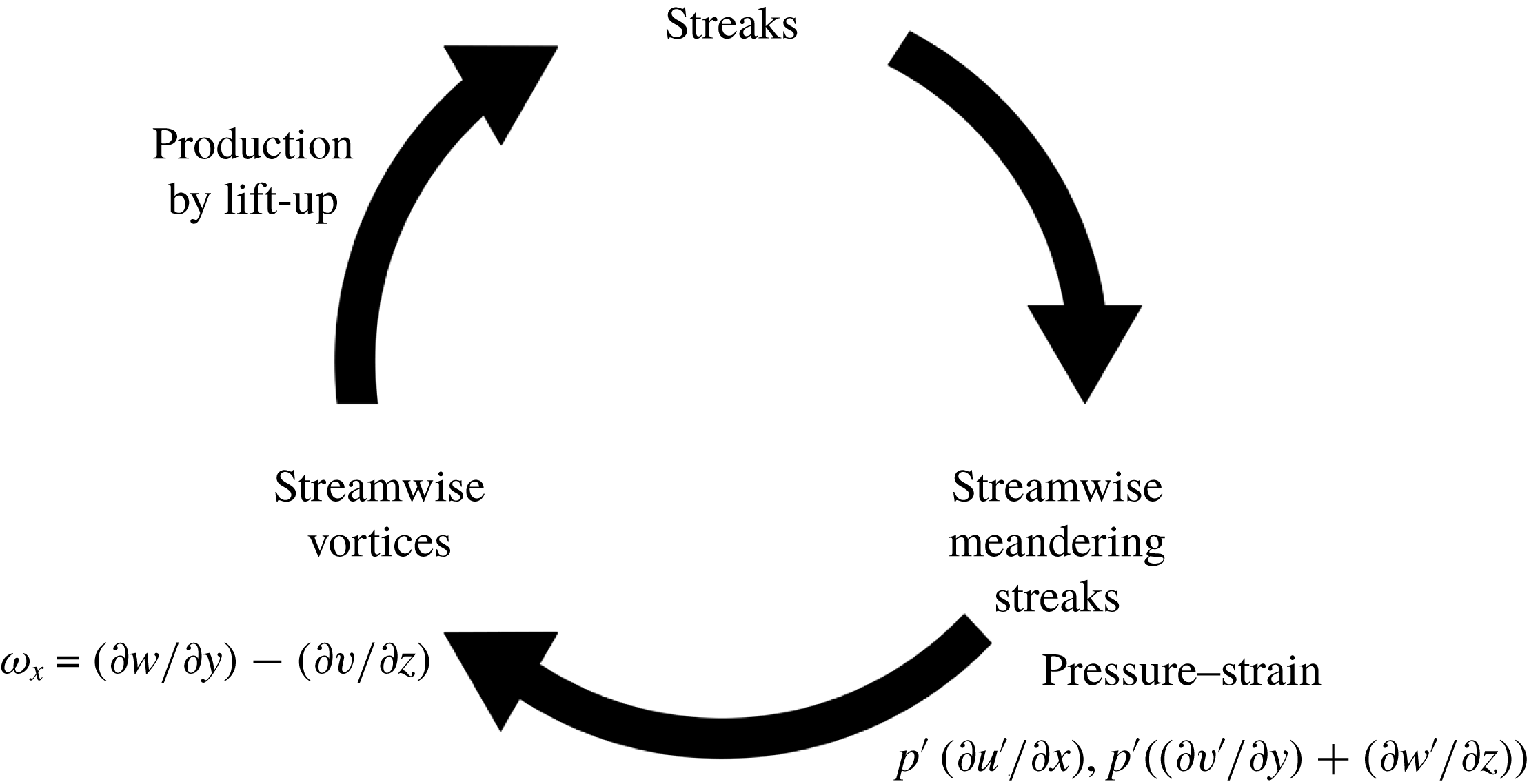
In figure 2(a), we have shown that the production spectra are well aligned along the linear ridge
 $\unicode[STIX]{x1D706}_{z}=5y$
. This suggests that the lift-up effect takes place in the form of Townsend’s attached eddies, consistent with the previous linear theory (Hwang & Cossu Reference Hwang and Cossu2010a
). However, the direct association of the lift-up effect with turbulence production itself does not necessarily indicate that the dominant dynamics of the energy-containing motions is governed by the self-sustaining process (e.g. Hamilton, Kim & Waleffe Reference Hamilton, Kim and Waleffe1995; Waleffe Reference Waleffe1997; Schoppa & Hussain Reference Schoppa and Hussain2002), as the lift-up effect is only a single element that constitutes the self-sustaining process (see also figure 14). Indeed, the streak amplification via the lift-up effect is possible whenever the driving nonlinearity can excite any wall-normal velocity, as previously shown with the stochastic response of the linearized Navier–Stokes equation (Gayme et al.
Reference Gayme, Mckeon, Papachristodoulou, Bamieh and Doyle2010; Hwang & Cossu Reference Hwang and Cossu2010a
). Therefore, without understanding of the origin of
 $v^{\prime }$
, the link between lift-up effect and turbulence production alone does not lead to the conclusion that the self-sustaining process is directly involved in turbulence production.
The better understanding of the origin of
 $v^{\prime }$
is gained by inspecting pressure–strain spectra in figure 9. The streamwise component of the pressure–strain spectra is shown to be aligned along
 $\unicode[STIX]{x1D706}_{z}=5y$
(figure 9
a), the linear ridge associated with production spectra (figure 2
a). Consequently, the wall-normal and spanwise components of the pressure–strain spectra should be well aligned along the same linear ridge
 $\unicode[STIX]{x1D706}_{z}=5y$
(figure 9
b,c) because all the pressure–strain terms in (3.4) are only a function of the given spanwise wavenumber
 $k_{z}$
and they should satisfy (3.5). These features imply that the distribution of the streamwise TKE generated by turbulence production to the cross-streamwise TKE takes place at the integral length scale, as in the self-sustaining process. Furthermore, the streamwise component of pressure–strain terms is composed of
 $p^{\prime }$
and
 $\unicode[STIX]{x2202}u^{\prime }/\unicode[STIX]{x2202}x$
, indicating that the distribution of the streamwise TKE to the other components is possible only if
 $\unicode[STIX]{x2202}u^{\prime }/\unicode[STIX]{x2202}x$
is present. The presence of
 $\unicode[STIX]{x2202}u^{\prime }/\unicode[STIX]{x2202}x$
in the streamwise pressure–strain is reminiscent of the streak instability (Hamilton et al.
Reference Hamilton, Kim and Waleffe1995; Schoppa & Hussain Reference Schoppa and Hussain2002; Cassinelli, de Giovanetti & Hwang Reference Cassinelli, de Giovanetti and Hwang2017) and the following vortex stretching in the self-sustaining process (Schoppa & Hussain Reference Schoppa and Hussain2002), as it represents the meandering motion of streaks (Hwang & Bengana Reference Hwang and Bengana2016). Indeed, it was recently shown that the streak instability exists for the large-scale outer structures, and, in particular, it acts as the seeding mechanism of the large-scale motion (Kovasznay, Kibens & Blackwelder Reference Kovasznay, Kibens and Blackwelder1970) that carries an intense cross-streamwise TKE (de Giovanetti et al.
Reference de Giovanetti, Sung and Hwang2017).
Lastly, the form of the streamwise component of pressure–strain terms suggests that any efficient distribution of the streamwise TKE to the other components requires a strong correlation between
 $p^{\prime }$
and
 $\unicode[STIX]{x2202}u^{\prime }/\unicode[STIX]{x2202}x$
. The continuity then automatically ensures a strong correlation between
 $p^{\prime }$
and
 $\unicode[STIX]{x2202}v^{\prime }/\unicode[STIX]{x2202}y$
or between
 $p^{\prime }$
and
 $\unicode[STIX]{x2202}w^{\prime }/\unicode[STIX]{x2202}z$
(i.e. correlation with the cross-streamwise velocity components). In this respect, it would also be interesting to examine how these correlations are related to the self-sustaining process. Our preliminary investigation has recently revealed that both rapid and slow pressures are strongly correlated with the streak instability and the regeneration of the streamwise vortices in the self-sustaining process (Cho, Choi & Hwang Reference Cho, Choi and Hwang2016). This observation finally enables us to propose a schematic diagram of turbulence production and energy distribution in the self-sustaining process, as depicted in figure 14. This is, however, not a complete picture of the entire process yet, and a detailed investigation on the role of the pressure in the self-sustaining process is currently underway.
5 Concluding remarks
In the present study, we have investigated the spectral energy transfer process and scale interactions in a turbulent channel flow using the equation for spectral TKE. The main findings are summarized as follows:
(i) One-dimensional spanwise wavenumber spectra of each constituent in the spectral TKE equation (2.5) have been investigated: (a) turbulent production is uniformly distributed especially in the log region and the relevant spanwise length scale is proportional to the wall-normal distance; (b) the related spanwise length scale of the dissipation spectra is proportional to the Kolmogorov length scale; (c) the produced TKE in the log and outer regions is mainly balanced with turbulent transport at the integral length scales, and is transferred to the other length scales, at which the turbulent transport spectra are positive (Richardson–Kolmogorov energy cascade).
(ii) The visualization of triadic interactions in turbulent transport has confirmed that the dominant transfer mechanism is the classical energy cascade. In addition to this, two new types of scale interaction processes in the near-wall region have been revealed. First, the interactions between larger energy-containing motions are found to be involved in the process of the energy cascade from relatively small energy-containing motions. This is proposed to be linked to skin-friction generation by large energy-containing motions. Second, the downward positive energy transfer processes from small to large scales in the streamwise and spanwise velocity components are identified. It is shown that the formation and scaling of the wall-reaching inactive part of large energy-containing motions (Townsend Reference Townsend1976) are strongly related to this near-wall positive turbulent transport.
(iii) Finally, the analysis of the pressure–strain spectra and the relation between the TKE production and lift-up effect have indicated that the self-sustaining process is presumably the dominant dynamics of the energy-containing motions given in the form of Townsend’s attached eddies.
Acknowledgements
This work was supported by the National Research Foundation through the Ministry of Science and ICT (NRF-2016R1E1A1A02921549 and NRF-2017R1A4A1015523). Y.H. is supported by the Engineering and Physical Sciences Research Council (EPSRC) in the UK (EP/N019342/1).