2 LST analysis

Consider a two-dimensional supersonic flow on a flat plate. The flow velocity, pressure and temperature are scaled using their free-stream values as: $(u,v)=(u^{\ast },v^{\ast })/U_{\infty }^{\ast }$ , $p=p^{\ast }/(\unicode[STIX]{x1D70C}_{\infty }^{\ast }U_{\infty }^{\ast 2})$ , $T=T^{\ast }/T_{\infty }^{\ast }$ . The non-dimensional streamwise and vertical coordinates are $(x,y)=(x^{\ast },y^{\ast })/L^{\ast }$ and time is $t=t^{\ast }U_{\infty }^{\ast }/L^{\ast }$ , where $L^{\ast }$ is the distance from the plate leading edge and asterisks denote dimensional quantities. It is assumed that the Reynolds number $Re=U_{\infty }^{\ast }\unicode[STIX]{x1D70C}_{\infty }^{\ast }L^{\ast }/\unicode[STIX]{x1D707}_{\infty }^{\ast }$ is sufficiently large to neglect the viscous–inviscid interaction effect; i.e. the shock wave induced by the boundary layer is weak and the flow parameters at the upper boundary-layer edge are equal to the corresponding free-stream parameters. The boundary-layer profiles of basic (or undisturbed) flow are approximated by the compressible Blasius solutions $U(\unicode[STIX]{x1D702})$ and $T(\unicode[STIX]{x1D702})$ , where $\unicode[STIX]{x1D702}=y(Re/x)^{1/2}$ .

Consider a small unsteady disturbance, which is described by the vector function

(2.1) $$\begin{eqnarray}\displaystyle \boldsymbol{Q}(x,y,t)=(u^{\prime },\unicode[STIX]{x2202}u^{\prime }/\unicode[STIX]{x2202}y,v^{\prime },p^{\prime },T^{\prime },\unicode[STIX]{x2202}T^{\prime }/\unicode[STIX]{x2202}y)^{\text{T}}. & & \displaystyle\end{eqnarray}$$

In the framework of spatial LST and using the local-parallel approximation (for $Re^{1/2}\gg 1$ ), the amplitude function $\boldsymbol{Q}$ is approximated as

(2.2) $$\begin{eqnarray}\displaystyle \boldsymbol{Q}(x,y,t)=\hat{\boldsymbol{q}}(Y;\unicode[STIX]{x1D714},x)\text{e}^{\text{i}\unicode[STIX]{x1D6F7}},\quad \unicode[STIX]{x1D6F7}=\int _{x_{0}}^{x}\unicode[STIX]{x1D6FC}(x,\unicode[STIX]{x1D714})\,\text{d}x, & & \displaystyle\end{eqnarray}$$

where $Y=Re^{1/2}y$ is the boundary-layer coordinate, $\unicode[STIX]{x1D714}$ is circular frequency which is expressed in terms of the frequency parameter $F=\unicode[STIX]{x1D714}^{\ast }\unicode[STIX]{x1D707}_{\infty }^{\ast }/(\unicode[STIX]{x1D70C}_{\infty }^{\ast }U_{\infty }^{\ast 2})$ as $\unicode[STIX]{x1D714}=F\times Re$ , $\unicode[STIX]{x1D6FC}=\unicode[STIX]{x1D6FC}^{\ast }L^{\ast }$ is the streamwise wavenumber, the shape function $\hat{\boldsymbol{q}}(Y;\unicode[STIX]{x1D714},x)$ depends on $x$ parametrically and satisfies the system of linear stability equations

(2.3) $$\begin{eqnarray}\displaystyle \frac{\text{d}\hat{\boldsymbol{q}}}{\text{d}Y}=\mathbb{H}\hat{\boldsymbol{q}}. & & \displaystyle\end{eqnarray}$$

Here $\mathbb{H}$ is a $6\times 6$ matrix, whose explicit form can be found in works of Nayfeh (Reference Nayfeh1980), Fedorov (Reference Fedorov2013) and many other papers. The boundary conditions are the no-slip condition on an isothermal wall and the boundedness of disturbance in the outer inviscid flow

(2.4) $$\begin{eqnarray}\displaystyle & \displaystyle y=0:\hat{u} =\hat{v}=\hat{T}=0, & \displaystyle\end{eqnarray}$$

(2.5) $$\begin{eqnarray}\displaystyle & \displaystyle y\rightarrow \infty :|\hat{u} ,\hat{v},\hat{T}|<\infty . & \displaystyle\end{eqnarray}$$

Figure 1.

Schematic pattern of the continuous (lines) and discrete (crosses) spectra in the complex $\unicode[STIX]{x1D6FC}$ -plane at a fixed and real frequency $\unicode[STIX]{x1D714}$ ; $\unicode[STIX]{x1D6FC}_{c,1}^{+}$ – vorticity waves, $\unicode[STIX]{x1D6FC}_{c,2}^{+}$ – entropy waves, $\unicode[STIX]{x1D6FC}_{c,3}^{+}$ , $\unicode[STIX]{x1D6FC}_{c,4}^{+}$ – acoustic waves, $\unicode[STIX]{x1D6FC}_{c,1,2,3}^{-}$ – waves propagating upstream, $\unicode[STIX]{x1D6FC}_{n}$ – normal modes of discrete spectrum.

The discrete and continuous spectra $\unicode[STIX]{x1D6FC}(\unicode[STIX]{x1D714})$ of the problem (2.3)–(2.5) have been studied by Tumin & Fedorov (Reference Tumin and Fedorov1983) and Balakumar & Malik (Reference Balakumar and Malik1992). It was shown that besides the discrete spectrum $\unicode[STIX]{x1D6FC}_{n}(\unicode[STIX]{x1D714})$ , which satisfies the boundary condition $\hat{u} ,\hat{v},\hat{T}\rightarrow 0$ for $y\rightarrow \infty$ , there are seven branches of the continuous spectrum (see figure 1). The three branches $\unicode[STIX]{x1D6FC}_{c,1}^{-},\unicode[STIX]{x1D6FC}_{c,2}^{-},\unicode[STIX]{x1D6FC}_{c,3}^{-}$ correspond to waves propagating upstream with rapid decay. The two branches $\unicode[STIX]{x1D6FC}_{c,3}^{+},\unicode[STIX]{x1D6FC}_{c,4}^{+}$ correspond to acoustic waves propagating downstream

(2.6a,b ) $$\begin{eqnarray}\displaystyle \unicode[STIX]{x1D6FC}_{c,3}^{+}=\frac{\unicode[STIX]{x1D714}M\cos \unicode[STIX]{x1D6E9}}{M\cos \unicode[STIX]{x1D6E9}-1}+O(Re^{-1}),\quad \unicode[STIX]{x1D6FC}_{c,4}^{+}=\frac{\unicode[STIX]{x1D714}M\cos \unicode[STIX]{x1D6E9}}{M\cos \unicode[STIX]{x1D6E9}+1}+O(Re^{-1}), & & \displaystyle\end{eqnarray}$$

where $\unicode[STIX]{x1D6E9}$ is the angle between the wave front and the $y$ -axis, and $M$ is free-stream Mach number. The phase speed, $c=\unicode[STIX]{x1D714}/\unicode[STIX]{x1D6FC}$ , is in the range of $c_{r}\leqslant 1-1/M$ for slow waves and $c_{r}\geqslant 1+1/M$ for fast waves. The two branches $\unicode[STIX]{x1D6FC}_{c,1}^{+},\unicode[STIX]{x1D6FC}_{c,2}^{+}$ correspond to vorticity and entropy waves propagating downstream with the phase speed $c_{r}=1+O(Re^{-1/2})$ . Hereafter the subscripts ‘ $r$ ’ and ‘ $i$ ’ stand for real and imaginary parts of complex values respectively.

For the boundary layer considered herein, there are two unstable modes of the discrete spectrum: the first mode related to Tollmien–Schlichting waves at subsonic speeds and the Mack second mode of acoustic nature. The latter becomes the dominant instability at sufficiently large Mach numbers. Further discussion is focused on the Mack second mode and acoustic waves of the continuous spectrum.

As an example, we consider perfect gas of the specific heat ratio $\unicode[STIX]{x1D6FE}=1.4$ and Prandtl number $Pr=0.72$ . The dynamic viscosity is approximated by the Sutherland law

(2.7) $$\begin{eqnarray}\displaystyle \unicode[STIX]{x1D707}^{\ast }=\unicode[STIX]{x1D707}_{e}^{\ast }\frac{T_{e}^{\ast }+S^{\ast }}{T^{\ast }+S^{\ast }}\left(\frac{T^{\ast }}{T_{e}^{\ast }}\right)^{3/2}, & & \displaystyle\end{eqnarray}$$

where $S^{\ast }=110.4K$ . The bulk viscosity is supposed to be zero. The free-stream parameters are: Mach number $M=6$ , temperature $T_{\infty }^{\ast }=300$  K and the Reynolds number $Re=10^{6}$ . The plate surface is isothermal with the cold wall temperature $T_{w}^{\ast }=0.5T_{\infty }^{\ast }$ . The basic flow profiles $U(\unicode[STIX]{x1D702})$ and $T(\unicode[STIX]{x1D702})$ are shown by the lines in figure 2.

Figure 2.

Self-similar boundary-layer profiles; $\unicode[STIX]{x1D702}=y^{\ast }/\sqrt{\unicode[STIX]{x1D707}_{\infty }^{\ast }x^{\ast }/\unicode[STIX]{x1D70C}_{\infty }^{\ast }U_{\infty }^{\ast }}$ is Blasius coordinate, HSFlow is Navier–Stokes solution.

Figure 3.

Growth rates (a) and the phase speeds (b) of the Mack second-mode waves at various frequency parameters $F$ . The bold line shows the branch cut of slow acoustic waves.

Figure 3(a) shows the spatial growth rates $\unicode[STIX]{x1D70E}=-\unicode[STIX]{x1D6FC}_{i}$ of the Mack second mode versus the streamwise coordinate $x$ at various values of the frequency parameter $F$ . In figure 3(b), the black lines are the corresponding trajectories in the complex $(c_{r},c_{i})$ plane, while the bold line shows an approximate location of the branch cut related to the slow acoustic waves. As contrasted to the case of high-frequency waves (lines 1–4), the dispersion curves at relatively low frequencies (lines 5–10) have a kink near the point where $c=1-1/M$ . Further downstream the low-frequency waves travel supersonically relative to the outer inviscid flow. Their growth rate varies slowly versus $x$ and ultimately the dispersion curves coalesce with the branch cut of slow acoustic waves.

Figure 4.

Trajectories of the low-frequency wave of $F=1.3124\times 10^{-4}$ (a) and the high-frequency wave of $F=2.059\times 10^{-4}$ (b) in the complex $c$ -plane for the Mack second mode (thin solid lines). The dashed line shows the trajectory of new stable mode.

More details on the behaviour of low-frequency and high-frequency unstable waves are given in figure 4(a,b) showing the trajectories in the $(c_{r},c_{i})$ plane. The low-frequency wave (figure 4 a) originates at the branch point $c_{F}=1+1/M$ of fast acoustic waves (this occurs at $x\rightarrow 0$ ). As indicated by arrows, the phase speed reduces and the wave becomes damped as $x$ is increased. Then, the phase-speed trajectory crosses the branch cut of the vorticity/entropy waves at $c_{r}\approx 1$ . This phenomenon was explored by Fedorov & Khokhlov (Reference Fedorov and Khokhlov2001), Fedorov & Tumin (Reference Fedorov and Tumin2003). As $x$ is increased further, the wave becomes unstable and remains unstable passing above the branch point $c_{S}=1-1/M$ of slow acoustic waves. Eventually the phase-speed trajectory coalesces with the upper side of the branch cut at $c_{s}\approx c_{sr}\approx 0.76$ . In the vicinity of the branch point $c_{S}$ , where the phase-speed trajectory has a kink, a new stable mode of the discrete spectrum is formed. Its trajectory is shown by the dashed line in figure 4(a).

The phase-speed trajectory of the high-frequency wave (figure 4 b) is qualitatively different. It originates in the vicinity of the branch point $c_{S}$ . As $x$ is increased, this wave becomes unstable and, then, it becomes stable again before its phase speed falls below $c_{S}$ . Although the trajectory does not coalesce with the branch cut of slow acoustic waves, it passes in the close neighbourhood of the branch point $c_{S}$ .

Figure 5.

The pressure field of the second-mode wave at the coalescence point $x\approx 5.59$ (a), and at the mid-point of synchronization region $x\approx 5.00$ (b), $(\unicode[STIX]{x1D709},\unicode[STIX]{x1D702})=(x^{\ast },y^{\ast })/\sqrt{\unicode[STIX]{x1D708}_{\infty }^{\ast }x^{\ast }/U_{\infty }^{\ast }}$ . In the outer flow ( $\unicode[STIX]{x1D702}>10$ ), the front angle of radiated acoustic wave is $\unicode[STIX]{x1D6E9}\approx 46.5^{\circ }$ in case (a) and $\unicode[STIX]{x1D6E9}\approx 35.9^{\circ }$ in case (b). The boundary-layer thickness is $\unicode[STIX]{x1D702}_{\unicode[STIX]{x1D6FF}}(U=0.99U_{\infty })\approx 7.5$ .

Figure 4(a) also shows that the second-mode phase speed is very close to the branch cut of slow acoustic waves in the range $c_{sr}<c_{r}<1-1/M$ corresponding to the region $4.47<x<5.59$ (see line 6 in figure 3 a,b). On the basis of (2.6a,b ), the second mode should radiate almost neutral slow acoustic waves with the front angle increasing from $0^{\circ }$ (at $x\approx 4.47$ ) to $\unicode[STIX]{x1D6E9}_{s}\approx 46.5^{\circ }$ (at $x\approx 5.59$ ). This is confirmed by the local pressure-disturbance fields shown in figure 5(a) near the point of coalescence $x\approx 5.59$ , where $c=c_{s}\approx 0.758-\text{i}\times 8.509\times 10^{-6}$ , and in figure 5(b) near the mid-point $x=5$ , where $c\approx 0.794+\text{i}\times 1.693\times 10^{-4}$ . In the outer flow, the disturbance represents an inclined slow acoustic wave. Computations show that the vertical component of the energy flux vector of this wave is positive, $e_{y}=(\hat{v}_{r}\hat{p}_{r}+\hat{v}_{i}\hat{p}_{i})/2>0$ ; i.e. the wave propagates away from the wall.

Thus, the linear stability theory predicts that the Mack second mode propagating in the boundary layer on a sufficiently cold plate should radiate slow acoustic waves in the low-frequency band. Note that this phenomenon, which is called as a spontaneous radiation (or emission) of sound, was discussed by Landau & Lifshitz (Reference Landau and Lifshitz1987) in connection with the corrugation instability of shock waves. In the next section, the foregoing theoretical predictions are validated by direct numerical simulations.

3 Numerical studies

Direct numerical simulations (DNS) are performed using the in-house code HSFlow. It solves a full set of compressible Navier–Stokes equations using the fully implicit conservative total variation diminishing (TVD) shock-capturing scheme of second order in time. The advection terms are approximated by the third-order weighted essentially non-oscillatory (WENO) scheme (Jiang & Shu Reference Jiang and Shu1996). More details on the numerical method can be found in Egorov, Fedorov & Soudakov (Reference Egorov, Fedorov and Soudakov2006). Although the computational scheme is dissipative, its numerical dissipation can be reduced using a sufficiently fine computational grid. This allows for reliable numerical simulations of the boundary-layer stability and receptivity (Egorov et al. Reference Egorov, Fedorov and Soudakov2006; Egorov, Fedorov & Soudakov Reference Egorov, Fedorov and Soudakov2008; Fedorov et al. Reference Fedorov, Ryzhov, Soudakov and Utyuzhnikov2013).

The gas properties and free-stream conditions correspond to those specified in § 2. The computational domain is a rectangle ( $0\leqslant x\leqslant L_{x},0\leqslant y\leqslant L_{y}$ ) with its bottom side corresponding to the plate surface. The upper boundary is located above the plate-induced shock wave. The boundary conditions on the plate surface are the no-slip condition $(u,v)=(0,0)$ and the isothermal condition $T=T_{w}$ . On the inflow (left) and upper boundaries, the conditions correspond to the undisturbed free stream. On the outflow (right) boundary, the dependent variables $(u,v,p,T)$ are extrapolated using the linear approximation. In the cases considered, the induced disturbances propagate downstream and do not reach the upper boundary. Appreciable reflections from the outflow boundary are not observed because the flow is supersonic everywhere besides a thin near-wall layer. In this subsonic layer, the outflow boundary condition slightly affects the solution. However, this effect is rather local – the flow is perturbed upstream to a distance of approximately five grid cells near the wall. This small region is not involved into analysis of the disturbance field.

First, a steady-state solution is calculated with a high accuracy to provide the basic (undisturbed) flow field. The flow is assumed to be steady when the relative change of every flow variable $(u,v,p,T)$ is less than $10^{-8}$ during any time interval $\unicode[STIX]{x0394}t=1$ . Figure 2 shows that the $u$ and $T$ profiles of this solution (symbols) at $x=4$ agree well with the self-similar boundary-layer profiles (lines) used in the LST analysis of § 2. Similar agreements are observed at $x=0.5,2.0,6.0$ . The flow parameters at the upper boundary-layer edge are very close to the corresponding free-stream parameters: $U_{e}\approx 1.000$ , $M_{e}\approx 5.985$ , $T_{e}\approx 1.005$ . This confirms that the viscous–inviscid interaction is negligible.

Second, unsteady perturbations are imposed on the basic flow using the boundary condition

(3.1) $$\begin{eqnarray}\displaystyle \left.\begin{array}{@{}c@{}}(\unicode[STIX]{x1D70C}v)^{\prime }=\unicode[STIX]{x1D700}\sin (\unicode[STIX]{x1D6FC}_{c}(x-x_{0}))\sin (\unicode[STIX]{x1D714}_{c}t),\\ y=0,\quad x\in (x_{0},x_{0}+2\unicode[STIX]{x03C0}/\unicode[STIX]{x1D6FC}_{c}),\quad t\in (0,t_{max}),\end{array}\right\} & & \displaystyle\end{eqnarray}$$

which mimics a suction–blowing actuator. Here the initial point $x_{0}$ is chosen to be close to the neutral point of the second-mode wave of frequency $\unicode[STIX]{x1D714}_{c}$ , $2\unicode[STIX]{x03C0}/\unicode[STIX]{x1D6FC}_{c}$ is a streamwise length of the suction–blowing region which corresponds to the wavelength of disturbance at frequency $\unicode[STIX]{x1D714}_{c}$ and phase speed $c=1$ . Small parameter $\unicode[STIX]{x1D700}$ characterizes the amplitude of vertical mass-flow rate $(\unicode[STIX]{x1D70C}v)^{\prime }$ .

Third, the flow disturbance field $(u^{\prime },v^{\prime },p^{\prime },T^{\prime })$ is calculated by subtracting the steady-state solution from the unsteady solution.

Numerical simulations are performed for wave trains induced by the actuator working permanently ( $t_{max}\rightarrow \infty$ ) and wave packets induced by the actuator working during two periods ( $t_{max}=4\unicode[STIX]{x03C0}/\unicode[STIX]{x1D714}_{c}$ ). In the both cases, two frequencies are considered: $\unicode[STIX]{x1D714}_{c}=131.24$ ( $F=1.3124\times 10^{-4}$ ) is relevant to a low-frequency (LF) disturbance with the phase-speed trajectory shown in figure 4(a) and $\unicode[STIX]{x1D714}_{c}=205.90$ ( $F=2.0590\times 10^{-4}$ ) is relevant to a high-frequency (HF) disturbance with the phase-speed trajectory shown in figure 4(b). For all cases considered, the forcing amplitude $\unicode[STIX]{x1D700}=10^{-4}$ is chosen to be sufficiently small to avoid the nonlinear effects. The forcing parameters are summarized in table 1.

Figure 6.

Spatial (a) and temporal (b) structure of the suction–blowing actuator; 1 – shape function, 2 – its Fourier transform.

Table 1.

Parameters of the suction–blowing actuator for low-frequency (LF) and high-frequency (HF) disturbances.

The $x$ -shape of the suction–blowing actuator, $f(\unicode[STIX]{x1D701})=\sin (2\unicode[STIX]{x03C0}\unicode[STIX]{x1D701}),\unicode[STIX]{x1D701}=\unicode[STIX]{x1D6FC}_{c}(x-x_{0})/(2\unicode[STIX]{x03C0})$ and its Fourier transform,

(3.2) $$\begin{eqnarray}\displaystyle \hat{f}(\bar{\unicode[STIX]{x1D6FC}})=\int _{-\infty }^{+\infty }f(\unicode[STIX]{x1D701})\text{e}^{-\text{i}\bar{\unicode[STIX]{x1D6FC}}\unicode[STIX]{x1D701}}\,\text{d}\unicode[STIX]{x1D701},\quad \bar{\unicode[STIX]{x1D6FC}}=\unicode[STIX]{x1D6FC}/\unicode[STIX]{x1D6FC}_{c}, & & \displaystyle\end{eqnarray}$$

are shown in figure 6(a). The $t$ -shape, $f(\unicode[STIX]{x1D70F})=\sin (2\unicode[STIX]{x03C0}\unicode[STIX]{x1D70F}),\unicode[STIX]{x1D70F}=\unicode[STIX]{x1D714}_{c}t/(2\unicode[STIX]{x03C0})$ and its Fourier transform,

(3.3) $$\begin{eqnarray}\displaystyle \hat{f}(\bar{\unicode[STIX]{x1D714}})=\int _{-\infty }^{+\infty }f(\unicode[STIX]{x1D70F})\text{e}^{\text{i}\bar{\unicode[STIX]{x1D714}}\unicode[STIX]{x1D70F}}\,\text{d}\unicode[STIX]{x1D70F},\quad \bar{\unicode[STIX]{x1D714}}=\unicode[STIX]{x1D714}/\unicode[STIX]{x1D714}_{c}, & & \displaystyle\end{eqnarray}$$

are shown in figure 6(b) and related to the simulations of wave packets ( $t_{max}=4\unicode[STIX]{x03C0}/\unicode[STIX]{x1D714}_{c}$ ).

The LF cases are simulated in the computational domain of $L_{x}\times L_{y}=7.0\times 1.5$ using a structured multi-block grid with rectangular cells and $N_{x}\times N_{y}=5001\times 1001$ nodes. The grid is clustered near the plate leading edge and in the vicinity of the wall. Downstream from the leading edge (for $x>0.05$ ) the grid nodes are evenly spaced in the both directions. Downstream from the actuator (for $x>x_{0}$ ) there are more than 270 grid nodes across the boundary layer.

Figure 7.

Numerical grid verification. $N_{x}=5001$ , $N_{y}=251$ (1), 501 (2), 1001 (3), 2001 (4).

Figure 8.

LF wave train: (a) pressure-disturbance field, (b) wall-pressure-disturbance distribution, (c) kink region close-up, $x_{k}\approx 4.5$ ; (d) synchronization region close-up, $x_{s}\approx 5.6$ .

In the case of LF wave train, the numerical solution was verified using a finer grid in $y$ . No significant difference in the pressure disturbance amplitude was observed for grids $5001\times 2001$ and $5001\times 1001$ (see figure 7). In both cases, there are about 27 grid nodes per the disturbance wavelength in $x$ -direction. With these grids the numerical dissipation leads to the disturbance amplitude attenuation of about 0.2 % per wavelength that is 10 times smaller than the characteristic growth of instability.

For the HF cases, the grid is obtained by scaling of the LF grid. Assuming that the disturbance phase speed is close to one, the scaling factor is chosen as $(\unicode[STIX]{x1D714}_{c})_{LF}/(\unicode[STIX]{x1D714}_{c})_{HF}\approx 0.64$ . All characteristic dimensions and time are scaled using this factor.

3.1 Wave trains

The pressure-disturbance field of the LF wave train is illustrated by figure 8(a–d). In accord with the LST analysis the disturbance grows exponentially in the boundary layer downstream of the actuator (figure 8 b). Near the point $x_{k}\approx 4.5$ where the phase-speed trajectory of the second mode has a kink (see figure 4 a), the wave train starts to penetrate into the outer flow (figure 8 c). In the region $4.5<x<5.6$ (which is called hereafter as a synchronization region) the wave train radiates slow acoustic waves propagating away the wall and forming an outer acoustic field (figure 8 a). In accordance with the LST prediction, the front angle of these waves increases from $\unicode[STIX]{x1D6E9}=0^{\circ }$ at $x=4.5$ (figure 8 c) to $\unicode[STIX]{x1D6E9}\approx 46^{\circ }$ at $x=5.6$ (figure 8 d). Close-up views of the pressure-disturbance field near these end points are shown in figure 8(c,d), respectively. These fields resemble the local fields predicted by LST (figure 5). Further downstream the power of the radiated field drops down; i.e. the spontaneous radiation of sound is localized in the synchronization region.

Figure 8(a) shows that the far field of pressure disturbance resembles a beam of slow acoustic waves with the front angle $\unicode[STIX]{x1D6E9}\approx 33^{\circ }$ . This beam is directed along the group velocity vector inclined with respect to the wall at the angle of approximately $6^{\circ }$ . Note that this angle is essentially smaller than the Mach wave angle $\sin ^{-1}(1/M)\approx 9.6^{\circ }$ . Below the beam, the acoustic field has a complicated pattern associated with the interference between monochromatic waves of different front angles and amplitudes. This might be due to the fact that the strongest radiation occurs in the vicinity of kink ( $x\approx 4.5$ ) and near the point of coalescence ( $x\approx 5.6$ ), where the synchronization between the second mode and sound waves is most prominent.

Figure 9.

LF wave train: (a) phase speed, (b) growth rate.

Figure 8(b) shows that the wall-pressure disturbance is almost neutral in the synchronization region, while the local-parallel LST analysis predicts a slight exponential growth. This discrepancy motivated us to perform stability computations including the non-parallel effect using the multiple-scale asymptotic approach (see, for example, Nayfeh Reference Nayfeh1980). Figure 9 compares the phase speed $c_{r}$ (a) and the growth rate $\unicode[STIX]{x1D70E}=-\unicode[STIX]{x1D6FC}_{i}$ (b) predicted by the local-parallel LST and the non-parallel stability theory (NLST) with the corresponding quantities predicted by DNS. The latter were extracted from instantaneous distributions of the wall-pressure disturbance. Near the kink point $x=x_{k}$ , where $\text{d}\unicode[STIX]{x1D70E}(x)/\text{d}x$ predicted by LST has a jump, the non-parallel correction is singular. Outside of this local region the phase speeds of LST and NLST agree well with that of DNS. The all three solutions indicate that the disturbance is supersonic downstream of the kink point, while in the region of $x<x_{k}$ , the NLST growth rate agrees satisfactorily with DNS. In the region of spontaneous radiation ( $x>x_{k}$ ), the agreement is only qualitative. Figure 10(a) shows that upstream of the spontaneous radiation region $(x<4.5)$ the wall-pressure disturbance amplifies in accord with the NLST. Further downstream the NLST solution continues to grow while the DNS solution does not. Presumably, this difference is due to the loss of disturbance energy via the radiation of acoustic waves into the outer flow. However, the data represented in log scale (figure 10 b) indicate that the stabilization effect is relatively weak.

Figure 10.

Distributions of the wall-pressure disturbance for LF wave train in linear (a) and logarithmic (b) scale.

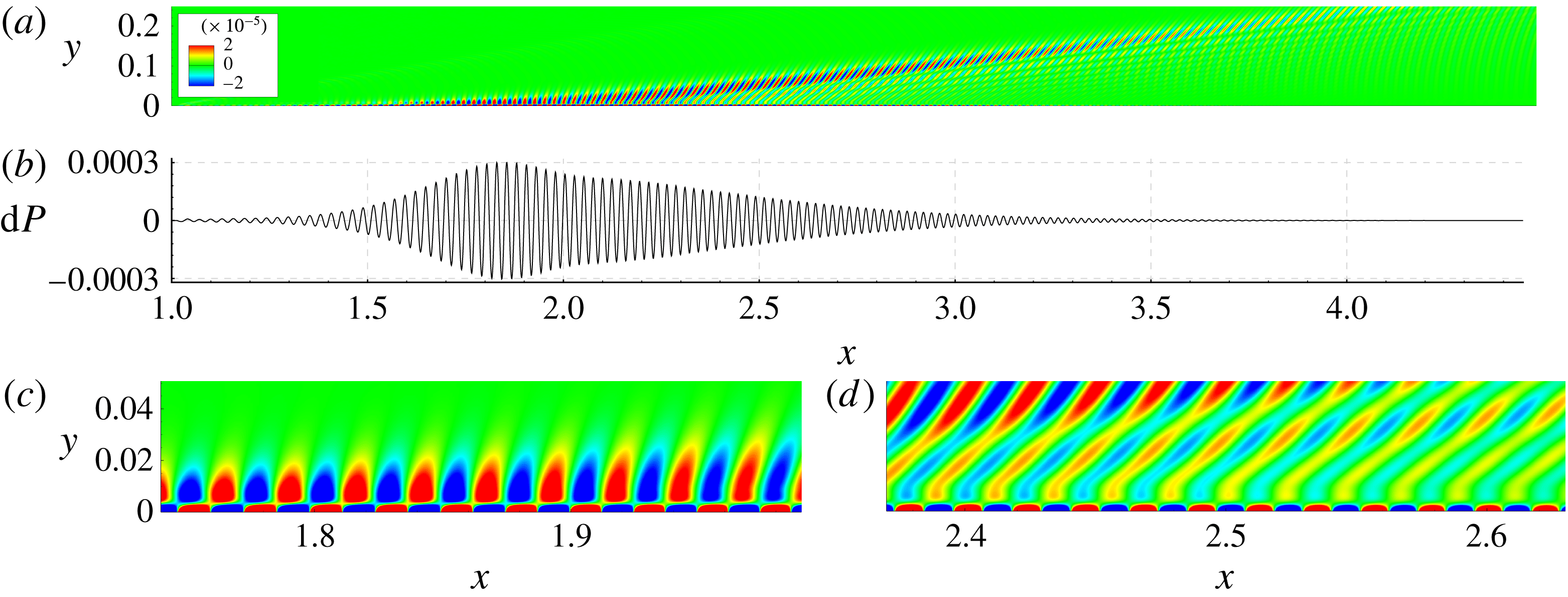
Figure 11(c,d) shows that the HF wave train radiates acoustic waves as well. This occurs near the point $x\approx 1.9$ where the phase-speed trajectory of the second mode is close to the branch cut of slow acoustic waves (see figure 4 b). Similar to the case of LF wave train, the far field looks like a beam with the dominant acoustic wave of $\unicode[STIX]{x1D6E9}\approx 39^{\circ }$ . However, the radiation region is essentially narrower and amplitudes of radiated sound are approximately 20 times smaller. The latter can be explained by the fact that, according to the LST predictions, the amplification of HF instability is about 18 times lower than that of LF instability. Below the acoustic beam, the wave fronts have a shape typical for slow acoustic waves radiated by a local harmonic source which is fixed in space. Presumably this source results from a spatial non-uniformity of the wave train in the synchronization region.

Figure 11.

HF wave train: (a) pressure-disturbance field, (b) wall-pressure-disturbance distribution, (c) synchronization region close-up, $x_{s}\approx 1.9$ ; (d) downstream region close-up.

3.2 Wave packets

Figure 12.

Phase speeds $c_{r}$ (a) and growth rates $\unicode[STIX]{x1D70E}$ (b) from LST for nearly adiabatic wall, $T_{w}/T_{e}=7$ .

In more realistic situations, the boundary-layer instability is observed as wave packets of broad-band frequency. First, consider the case of a nearly adiabatic wall, $T_{w}/T_{e}=7$ . The LST analysis shows that the second-mode waves are subsonic, and their phase speeds are far from those of slow acoustic waves (figure 12). In numerical simulations the wave packet is excited by the suction–blowing actuator (3.1) having the parameters: $x_{0}=1.0$ , $\unicode[STIX]{x1D700}=10^{-3}$ , $\unicode[STIX]{x1D714}_{c}=130.0$ and $\unicode[STIX]{x1D6FC}_{c}=\unicode[STIX]{x1D714}_{c}$ . The actuator works during half of a period ( $t_{max}=\unicode[STIX]{x03C0}/\unicode[STIX]{x1D714}_{c}$ ) and its $x$ -shape corresponds to that shown in figure 6 a). The DNS solution indicates that the wave packet does not radiate acoustic waves to the outer flow (figure 13, see supplementary movie 1, available at http://dx.doi.org/10.1017/jfm.2016.560). The instability propagates downstream in a usual manner – the wall-pressure fluctuation has a single-bell shape, with its carrier wavelength slowly increasing downstream.

Now consider the cases relevant to the cold wall of $T_{w}/T_{e}=0.5$ . The suction–blowing actuator works during two periods ( $t_{max}=4\unicode[STIX]{x03C0}/\unicode[STIX]{x1D714}_{c}$ ). Its other parameters are given in table 1. The frequency content of the actuator signal is shown in figure 6(b). The DNS results are shown in figures 14 and 15 for the LF and HF wave packet, respectively. In the both cases, qualitative features of the disturbance field are the same, while the quantitative difference is significant – the HF wave packet amplification is smaller and, therefore, the radiated acoustic field is weaker than in the case of LF wave packet.

Figure 13.

Wave packet on the near-adiabatic wall, $T_{w}/T_{e}=7$ at the time instants $t=5.0$ (a,b), 12.0 (c,d) and 19.0 (e,f); (a,c,e) pressure disturbance field, (b,d,f) wall-pressure-disturbance distribution, $\text{d}P=p_{w}^{\prime }$ . See supplementary movie 1.

Figure 14.

LF wave packet case. Different time instants: $t=2.0$ (a,b), 3.2 (c,d), 4.4 (e,f), 5.6 (g,h) and 6.8 (i,j); (a,c,e,g,i) pressure-disturbance field, isolines $\text{d}p=10^{-8}$ , (b,d,f,h,j) wall-pressure-disturbance distribution. See supplementary movie 2.

Consider the pressure-disturbance field induced by the LF wave packet (figure 14, see supplementary movie 2). At first, the actuator generates a weak acoustic wave associated with hemi-circular fronts as well as the second-mode wave packet growing in the boundary layer. The acoustic wave propagates downstream faster than the wave packet hump and, ultimately, becomes negligible. Moreover, the wave packet radiates slow acoustic waves of very small amplitude (see instantaneous pressure-disturbance fields at $t=2.0$ and 3.2). Presumably, this weak radiation is due to the non-parallel effect associated with the downstream growth of the boundary-layer thickness.

The first appreciable portion of sound is radiated at $t\approx 4.5$ . As the wave packet propagates further downstream, its amplitude increases while the amplitude of acoustic ‘spot’ remains almost constant. Since the spot head moves faster than the wave packet hump, the spot stretches downstream transforming to an acoustic beam. After a certain time interval the wave packet radiates the second acoustic spot (see the disturbance field at $t\approx 5.6$ ). The third portion of radiation is noticeable at $t\approx 6.8$ , etc. This cascade process leads to significant elongation of the original disturbance. A non-uniform distribution of the wave packet components and the interference between the radiated acoustic waves result in an intricate pattern of the outer acoustic field.

The acoustic radiation leads to beats of the disturbance within the boundary layer (see the wall-pressure distributions at $t\approx 5.6$ and $6.8$ ). Assume that the modulation length scale $\unicode[STIX]{x0394}x$ (the distance between neighbouring maxima of the disturbance amplitude envelope) is of the order of the streamwise length of the region where the carrier wave of the wave packet is synchronized with the corresponding acoustic wave. In the vicinity of synchronization point $x_{rad}$ , the second-mode wavenumber is approximated as $\unicode[STIX]{x1D6FC}=\unicode[STIX]{x1D6FC}_{a}+(\unicode[STIX]{x2202}\unicode[STIX]{x1D6FC}/\unicode[STIX]{x2202}x)(x_{rad})\unicode[STIX]{x0394}x+\cdots \,$ . In accord with (2.2), the difference between the second-mode eiconal and the acoustic wave eiconal behaves as $\unicode[STIX]{x0394}\unicode[STIX]{x1D6F7}=1/2(\unicode[STIX]{x2202}\unicode[STIX]{x1D6FC}/\unicode[STIX]{x2202}x)(x_{rad})(\unicode[STIX]{x0394}x)^{2}$ . The effective radiation of acoustic wave occurs for $|\unicode[STIX]{x0394}\unicode[STIX]{x1D6F7}|\leqslant 1$ ; i.e. the detuning of synchronization should be relatively small. Using this restriction, the modulation length scale can be estimated from the equation $1/2(\unicode[STIX]{x2202}\unicode[STIX]{x1D6FC}/\unicode[STIX]{x2202}x)(x_{rad})(\unicode[STIX]{x0394}x)^{2}\approx 1$ . For the compressible Blasius mean flow, the second-mode wavenumber is $\unicode[STIX]{x1D6FC}\approx \unicode[STIX]{x1D6FC}(x_{rad})\sqrt{x/x_{rad}}$ , where $\unicode[STIX]{x1D6FC}=\unicode[STIX]{x1D714}/c(x_{rad})$ , which gives $\unicode[STIX]{x0394}x\approx 2\sqrt{x_{rad}c(x_{rad})/\unicode[STIX]{x1D714}}$ . Taking into account that $c(x_{rad})\approx 1-1/M\approx 0.83$ we obtain: in the LF case of $\unicode[STIX]{x1D714}\approx 131$ and $x_{rad}\approx 5$ , $\unicode[STIX]{x0394}x\approx 0.36$ ; in the HF case of $\unicode[STIX]{x1D714}\approx 206$ , $x_{rad}\approx 2$ , $\unicode[STIX]{x0394}x\approx 0.18$ . These estimates agree well with the modulation length observed in the numerical solutions.

Figure 15.

HF wave packet case. Different time instants: $t=0.72$ (a,b), 1.48 (c,d), 2.24 (e,f), 3.00 (g,h), 3.76 (i,j) and 4.52 (k,l); (a,c,e,g,i,k) pressure-difference field, isolines $\text{d}p=10^{-8}$ , (b,d,f,h,j,l) wall-pressure-disturbance distribution.

Figure 16.

Amplification of the spectral components of the LF wave packet. The initial point is $x_{0}=2.5$ . Amplitudes are normalized at points of maximum growth rate predicted by NLST.

Figure 17.

Spectra of the LF wave packet in different $x$ -stations.

It was also found that Fourier components of the wave packet behave in agreement with the NLST predictions in a broad frequency band. Figure 16 shows the wall-pressure distributions of these components, where lines represent the DNS solution and symbols represent the NLST solution. The distributions are normalized such as $p_{w,NLST}^{\prime }=p_{w,DNS}^{\prime }$ at points $x_{max}(\unicode[STIX]{x1D714})$ where the NLST growth rate is maximal. Similar to the case of the LF wave train (figure 10) the NLST solutions deviate from DNS ones in the regions of spontaneous radiation – a weak stabilization effect is noticeable.

The spectral analysis of the DNS disturbance fields reveals that the wave packet dispersion becomes abnormal in the region of spontaneous radiation. Figure 17 shows spectra $A_{p}(\unicode[STIX]{x1D714})$ of the wall-pressure disturbance in different $x$ -stations for the LF wave packet. As the disturbance propagates downstream, its spectrum quickly spreads to the low-frequency band and attains several maxima. Although not shown here, the HF wave packet dispersion behaves similarly. Thus, the spontaneous radiation provides a mechanism which transfers the disturbance energy from high-frequency to low-frequency band. This mechanism produces significant effect – the maximum of the disturbance amplitude does not grow downstream as clearly seen in figure 14(f,h,j) ( $t=4.4$ , $5.6$ and $6.8$ ) and in figure 15(f,h,j,l) ( $t=2.24$ , $3.00$ , $3.76$ , $4.52$ ).

To illustrate this statement, consider the case of HF wave packet. With the assumption that the initial amplitude of wave packet components is constant at the actuator locus $x=x_{0}$ (the initial disturbance has a broad-band spectrum), the amplitude ratio of each component is calculated using LST as

(3.4) $$\begin{eqnarray}\displaystyle A(x)/A_{0}=\exp \left(-\int _{x_{0}}^{x}\unicode[STIX]{x1D6FC}_{i}(x,\unicode[STIX]{x1D714})\,\text{d}x\right). & & \displaystyle\end{eqnarray}$$

Here $A_{0}$ is chosen such that $A/A_{0}=1$ on the envelope of amplification curves at the point $x_{1}=1.9$ where the spontaneous radiation begins (see figure 15). An envelope of the distributions (3.4) represents a qualitative behaviour of the wave packet amplitude. This approach captures the selective amplification of the wave packet components and ignores the dispersion effects. The maximum amplitude of wall-pressure disturbance is also determined using the DNS solution at each $x$ -station and plotted versus $x$ using the same scaling. As shown in figure 18(a), the abnormal dispersion leads to a significant reduction of the instability growth compared with the LST prediction.

In the case of LF wave packet, the radiation begins near the point $x=5$ (figure 14). Using this point for normalization of the amplification curves, we obtain the distributions of $A/A_{0}$ shown in figure 18(b). The stabilization effect is observed for $x>5.5$ where the spontaneous radiation of sound is appreciable.

Thus, the abnormal dispersion leads to a significant reduction of instability growth in the spontaneous radiation region. This effect may delay the transition onset on a sufficiently cold plate despite the fact that the second mode is destabilized by the wall cooling.

Figure 18.

Amplification ratios of the wave packet components predicted by LST (solid lines) and the distribution of wave packet maxima predicted by DNS (dashed line); (a) HF wave packet; (b) LF wave packet.