2. SIGNAL AND CHANNEL MODEL

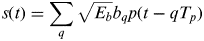
This section provides the time-frequency-based channel and signal models that underlie the development presented herein. The specular multipath channel considered here is assumed to be Wide Sense Stationary (WSS). The baseband signal at the transmitter side s(t) can be represented by

(1)$$s(t) = \sum\limits_q {\sqrt {E_b} b_q p(t - qT_p )} $$

where T _p is the code period duration, E _b is the bit energy and b _qs are the navigation data bits. p(t) is the spreading waveform with the chip interval of T _c and the autocorrelation function of g(τ). The signal bandwidth is $B \approx {\textstyle{1 \over {T_c}}} $ and the spreading factor of the system is $N_c = {\textstyle{{T_p} \over {T_c}}} \approx T_p B \gg 1$. The complex baseband signal x(t) at the output of the channel is related to the transmitted complex baseband signal s(t) by

(2)$$x(t) = \int {h(t,\tau )s(t - \tau )d\tau} + n(t)$$

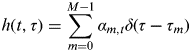
where h(t, τ) is the time-varying impulse response of the channel and n(t) is zero-mean, additive white circular Gaussian noise. The specular multipath channel with time variant coefficients can be modelled as

(3)$$h(t,\tau ) = \sum\limits_{m = 0}^{M - 1} {\alpha _{m,t} \delta (\tau - \tau _m )} $$

where δ(.) denotes the Dirac delta function, M is the total number of signal components including LOS, α _m,t and τ _m are the complex attenuation factor and the propagation delay of the m ^th path respectively (α _0,t and τ ₀ correspond to LOS).

An equivalent representation of the channel can be described in terms of the spreading function ψ(θ, τ), defined as

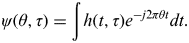(4)$$\psi (\theta, \tau ) = \int {h(t,\tau )e^{ - j2\pi \theta t} dt}. $$

Under the assumption that the observation time (integration time) is smaller than the coherence time of the channel, Equation (4) will result in

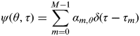(5)$$\psi (\theta, \tau ) = \sum\limits_{m = 0}^{M - 1} {\alpha _{m,\theta} \delta (\tau - \tau _m )} $$

where $\alpha _{m,\theta} = \int {\alpha _{m,t} e^{ - j2\pi t\theta}} $. The spreading function quantifies the time-frequency spreading produced by the channel, θ corresponds to the Doppler shifts introduced by the channel temporal variations and τ corresponds to the multipath delays. The time-varying channel impulse response ψ(θ,τ) is often modelled as a stochastic process and the wide-sense stationary uncorrelated scatters (WSSUS) model is widely used (Bello, Reference Bello1963). In this model, the temporal variations in ψ(θ,τ) are represented by a stationary Gaussian process and the channel response at different lags are assumed independent (Proakis, Reference Proakis1995). The second order statistics characterizing the channel are given by

(6)$$E\left\{ {\psi (\theta _1, \tau _1 )\psi ^ * (\theta _2, \tau _2 )} \right\} = E\left\{ {|\psi (\theta _1, \tau _1 )|^2} \right\}\delta (\theta _1 - \theta _2 )\delta (\tau _1 - \tau _2 ).} $$

The function ψ(θ,τ)=E{|ψ(θ,τ)|²} is called the scattering function (Sadowsky and KafedZiski, Reference Sadowsky and KafedZiski1998) and represents the distribution of channel power as a function of multipath and Doppler shifts. The support of this function over τ denoted by T _m is the delay spread of the channel and its support over θ, denoted by B _d, is the channel's Doppler spread. The Doppler spread of the channel is linearly proportional to the speed of the receiver and can be expressed as $B_d = {\textstyle{v \over \lambda}} $ (Rappaport, Reference Rappaport2002) where v is the speed of the receiver and λ is the wavelength of the signal.

3. DOPPLER-DELAY REPRESENTATION OF MULTIPATH SIGNAL

Considering the definitions in Equations (2–6), the received signal at the receiver consists of a linear combination of time shifted and frequency shifted copies of the transmitted signal. The Doppler frequency shifted copies of the transmitted signal produced by the fading channel (caused by user or caterer's motion) provide an inherent mechanism that can be exploited to improve the delay estimation accuracy via appropriate signal processing schemes. A representation of the received signal that provides a framework for exploiting this opportunity can be described as (Sayeed and Aazhang, Reference Sayeed and Aazhang1999)

(7)$$x(t) \approx \sum\limits_{k = - K}^K {\sum\limits_{m = 0}^{M - 1} {\psi \left( {\displaystyle{k \over T},\tau _m} \right)p(t - \tau _m )e^{\,j({{2\pi kt} / T})}}} + n(t)\quad 0 \leqslant t \lt T,} $$

where $K = \left\lceil {B_d T} \right\rceil $ and T is the coherent integration period. Considering the assumption of the statistical independence of the channel coefficients, ψ(θ,τ), the expression in Equation (7) effectively decomposes the channel into 2K+1 independent flat fading channels by appropriately sampling the multipath-Doppler plane. The number of these available channel copies is proportional to B _dT. For fixed channel parameters, this number is proportional to the time-bandwidth product of the signalling waveform. The approximation in Equation (7) can be made arbitrarily close by increasing the number of terms in the summation. However, virtually all the signal energy is captured by 2K +1 Doppler components.

Using Equation (7), the incoming signal after correlation with a replica of the modulated PRN code and sampling at the rate of F _s=1/T _s can be expressed as

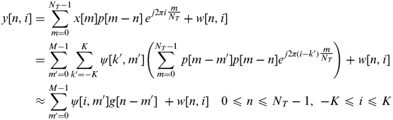(8)$$\eqalign{ \hskip-13pt y[n,i] &= \sum\limits_{m = 0}^{N_T - 1} {x[m]p[m - n]\,e^{\,j2\pi i\textstyle{m \over {N_T}}}} + w[n,i]\, \cr & = \sum\limits_{m' = 0}^{M - 1} {\sum\limits_{k' = - K}^K {\psi [k',m']} \left( {\sum\limits_{m = 0}^{N_T - 1} {\,p[m - m']p[m - n]e^{\,j2\pi (i - k')\textstyle{m \over {N_T}}}}} \right)} + w[n,i]\, \cr & \approx \sum\limits_{m' = 0}^{M - 1} {\psi [i,m']g[n - m']} \,\, + w[n,i] \quad 0 \leqslant n \leqslant N_T - 1,\,\, - K \leqslant i \leqslant K} $$

where n and i are the delay and frequency indexes respectively, $N_T = \left\lceil {\textstyle{T \over {T_s}}} \right\rceil $ and w is the noise term at the output of the correlator with a variance of $\sigma _w^2 = {\textstyle{{2N_0} \over {T_s}}} $. A matrix representation for the relation in Equation (8) can be expressed as

(9)$${\bf Y} = {\bf G\Psi} + {\bf W},$$

where Y is a N×(2K+1) matrix in which

(10)$${\bf Y}_{n,i} = y[n,i],$$

and $N = \left\lceil {\textstyle{{T_p} \over {T_s}}} \right\rceil $. G is an N×M matrix wherein

(11)$${\bf G}_{n,m} = g((n - m)T_s ),$$

ψ is the M×(2K+1) matrix described by

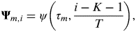(12)$${\bf \Psi} _{m,i} = \psi \left( {\tau _m, \displaystyle{{i - K - 1} \over T}} \right),$$

and finally W is the N×(2K+1) matrix of the noise samples at the output of the correlator with a covariance matrix of Q=σ _w²G′ where G′ is an L×L matrix that can be described as G′_n,m=g ((n−m)T _s).

4. SUBSPACE-BASED MULTIPATH DELAY ESTIMATION

In the previous section, it was shown that the output of the correlator in a fast fading channel can be represented as a matrix of independent samples for different values of the delay and Doppler shift. This matrix was shown to be linearly proportional to the matrix of scattering function of the channel. In this section, this time-frequency representation of the channel is employed to estimate the multipath times of arrival using the MUSIC technique.

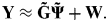
In Equation (9), every row of the scattering function matrix corresponds to one of the true multipath delays (τ _ms). Given that the true multipath delays are not known to the receiver beforehand, Equation (9) is rewritten for the receiver side considering an equi-spaced search region with a duration of Δ>max{τ ₁,…,τ _M} including $L = \left\lceil {\textstyle{\Delta \over {T_s}}} \right\rceil $ samples so that

(13)$${\bf Y} \approx {\bf \tilde G\tilde \Psi} + {\bf W}.$$

In Equation (13), assuming that the sampling period is small enough, the L×(2K+1) matrix ${\bf \tilde \Psi} $ is formed by adding some all-zero rows to ψ at the position of delays that do not correspond to the true multipath delay. Then, the k-th column of ${\bf \tilde \Psi} $, namely ${\bf \tilde \Psi} _k $, that contains the channel impulse response at the frequency shift of ${\textstyle{{k - K - 1} \over T}}$, by considering Equation (5), can be expressed as

(14)$${\bf \tilde \Psi} _k = [a_{1,k} \,\,a_{2,k} \,\,...\,\,a_{{\rm L},k} ]^T, $$

in which

(15)$$a_{i,k} = \left\{ {\matrix{ {\alpha _{m,k}} & {{\rm if}\,\,iT_s \simeq \tau _m \in \left\{ {\tau _0,..., \tau _{M - 1}} \right\}} \cr 0 & {{\rm otherwise}} \cr}} \right..$$

Also ${\bf \tilde G}$ in Equation (13) is an N×L matrix so that ${\bf \tilde G}_{n,m} = g((n - m)T_s )$.

Taking these into account, the rows of ${\bf \tilde \Psi} $ can be grouped into two sets. The first set includes the rows that correspond to the true multipath delays (τ _ms) and the second set includes the rest of the rows consisting of zero elements. Consequently, ${\bf \tilde \Psi} $ can be separated into two subsections as ${\bf \tilde \Psi} ^{(1)} $ (with M rows) and ${\bf \tilde \Psi} ^{(2)} $ (with L−M rows), corresponding to the first and second sets, respectively.

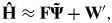
The MUSIC algorithm uses a coarse estimate of the Fourier transform of the ${\bf \tilde \Psi} _k $s to find an estimate for the multipath delays (Li and Pahlavan, Reference Li and Pahlavan2004). Assuming H to be a L×(2K+1) matrix whose k ^th column is the Fourier transform of ${\bf \tilde \Psi} _k $, a coarse estimate of this matrix (which can be obtained by a simple spectrum division (Klukas, Reference Klukas1997)) is expressed as

(16)$${\bf \hat H} \approx {\bf F\tilde \Psi} + {\bf W'},$$

where F is the L×L Discrete Fourier Transform (DFT) matrix so that ${\bf F}_{k,l} = e^{{{ - jkl}/ L}} $ and W′ is the L×(2K+1) noise matrix with a covariance matrix Q′=σ _w²I_L, where I_k indicates a k×k identity matrix. Considering the two subsections of ${\bf \tilde \Psi} $, and since the elements of ${\bf \tilde \Psi} ^{(2)} $ are zero, Equation (16) can be rewritten as

(17)$${\bf \hat H} \approx {\bf F}_1 {\bf \tilde \Psi} ^{(1)} + {\bf F}_2 {\bf \tilde \Psi} ^{(2)} + {\bf W'} = {\bf F}_1 {\bf \tilde \Psi} ^{(1)} + {\bf W'},$$

where F₁ is a subsection of F including those columns of F that correspond to the rows of ${\bf \tilde \Psi} ^{(1)} $. The other subsection of F that includes the columns of F corresponding to the rows of ${\bf \tilde \Psi} ^{(2)} $ is referred to as F₂. Moreover, since the columns of a DFT matrix are orthonormal, it can be shown that

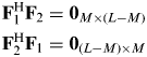(18)$$\eqalign{& {\bf F}_1^{\rm H} {\bf F}_2 = {\bf 0}_{M \times (L - M)} \cr & {\bf F}_2^{\rm H} {\bf F}_1 = {\bf 0}_{(L - M) \times M}} $$

where 0_a×b stand for a×b all zero matrix, and the superscript H denotes the Hermitian matrix transpose. Considering Equation (16), the estimated autocorrelation matrix of the measured data can be expressed as

(19)$${\bf \hat R} = {\bf \hat H\hat H}^{\rm H} = {\bf F}_1 {\bf AF}_1^{\rm H} + \sigma _w^2 {\bf G}$$

where A is a M×M matrix defined as

(20)$${\bf A} = {\bf \tilde \Psi} ^{(1)} \left({\bf \tilde \Psi} ^{(1)} \right)^{\rm H} = \sum\limits_{k = - K}^{k = - K} {{\bf \tilde \Psi} _k^{(1)} \left({\bf \tilde \Psi} _k^{(1)} \right)^{\rm H}}, $$

Since the columns of ${\bf \hat H}$ are the estimated channel frequency response at different Doppler frequency shifts, Equation (19) demonstrates the contribution of signals at different Doppler shifts in constructing the channel autocorrelation matrix and increasing its rank. In fact, different copies of the received signal in the Doppler-domain collaborate to make the rank of the signal subspace of the covariance matrix as close to the number of multipath components as possible. As shown in Figure 2, this improves the ability to recognize the multipath peaks from the noise peaks in the estimated delay profile. That is how the Doppler combining technique aids the estimation accuracy of the sub-space technique.

In the rest of this section, the Music algorithm for the discussed framework is explained for two different cases: when the matrix A is non-singular and when it is singular.

4.1. When matrix A is non-singular

The MUSIC super-resolution techniques are based on the eigen-decomposition of the autocorrelation matrix in Equation (19). In the case where A is non-singular (2K+1⩾M), since F₁ has a full column rank, the rank of F₁AF₁^H is M. Therefore, in this case, the L−M smallest eigenvalues of ${\bf \hat R}$ are equal to σ _w² and their corresponding eigenvectors (EVs) are called noise EVs, whereas EVs corresponding to the M largest eigenvalues are called signal EVs. Thus, the L-dimensional subspace that contains the signal vectors ${\bf \hat H}$ can be split into two orthogonal subspaces, known as the signal subspace U_s and the noise subspace U_N, by the signal EVs and noise EVs, respectively. Taking this into account, the autocorrelation matrix in Equation (19) can be written as

(21)$${\bf \hat R} = {\bf U\Lambda U}^H = [\matrix{ {{\bf U}_S} & {{\bf U}_N} \cr} ]\left[ {\matrix{ {{\bf \Lambda} _S + \sigma _w^2 {\bf I}_M} & 0 \cr 0 & {\sigma _w^2 {\bf I}_{L - M}} \cr}} \right]\left[ {\matrix{ {{\bf U}_S} \cr {{\bf U}_N} \cr}} \right],$$

where Λ_s is a diagonal matrix containing the signal eigenvalues on its diagonal. The signal and noise subspace matrixes have the following properties:

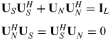(22)$$\eqalign{& {\bf U}_S {\bf U}_S^H + {\bf U}_N {\bf U}_N^H = {\bf I}_L \cr & {\bf U}_N^H {\bf U}_S^{} = {\bf U}_S^H {\bf U}_N^{} = 0} $$

and Equation (19) can therefore be rewritten as

(23)$${\bf \hat R} = {\bf U}_S {\bf \Lambda} _S {\bf U}_S^H + \sigma _w^2 {\bf UU}^H = {\bf U}_S {\bf \Lambda} _S {\bf U}_S^H + \sigma _w^2 {\bf I}_L. $$

Comparing Equation (23) with Equation (19) results in

(24)$${\bf U}_S {\bf \Lambda} _S {\bf U}_S^H = {\bf F}_1 {\bf AF}_1^H. $$

Hence, since A was assumed non-singular, the columns of F₁ span the signal subspace and are orthogonal to the noise subspace. Therefore, the projection matrix of the noise subspace, 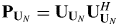${\bf P}_{{\bf U}_N} = {\bf U}_{{\bf U}_N} {\bf U}_{{\bf U}_N} ^H $, is orthogonal to F₁ which is expressed as

(25)$${\bf P}_{{\bf U}_N} {\bf F}_1 = 0.$$

Equation (25) implies that those columns of F that correspond to the true multipath delays are orthogonal to the noise subspace. Thus, the multipath delays, τ ₁,…, τ _M, can be determined by finding the delay values at which the following MUSIC Super-resolution Delay Profile (SDP) achieves its maximum values, namely

(26)$$SDP(\tau _i ) = \displaystyle{1 \over {\left\| {{\bf P}_{{\bf U}_N} {\bf F}_{\tau _i}} \right\|^2}} = \displaystyle{1 \over {{\bf F}_{\tau _i} ^H {\bf P}_{{\bf U}_N} {\bf F}_{\tau _i}}} = \displaystyle{1 \over {\left\| {{\bf U}_N^H {\bf F}_{\tau _i}} \right\|^2}}, $$

where ${\bf F}_{\tau _i} $ denotes the i-th column of F that corresponds to τ _i=iT _s. It should be noted here that Equation (25), which is the basis of multipath delay estimation by the function in Equation (26), holds only when the matrix A is non-singular. This is valid when the number of linearly independent copies of the signal that contribute to the computation of the autocorrelation matrix, which is the number coarse estimates of CFR on the columns of ${\bf \hat H}$, is larger than the number of multipath components. This is how independent estimates of CFR at different Doppler frequencies aim to increase the rank of A. It is important to consider the problem that arises if A is singular which will be explained in the next sub-section.

It should be noted at this point that when applying the various diversity techniques, Equation (26) is used exactly in the same way. The only difference is in the formation of the autocorrelation matrix in Equation (19). For example, in time diversity the columns of ${ \bf \hat H}}$ are the coarse estimates of CFR at consecutive time snapshots with a duration of T and for spatial diversity they are the coarse estimate of CFR at the different receiver antennas. Spatial-temporal diversity is the same as time diversity when the receiver is in motion (Broumandan et al., Reference Broumandan, Nielsen and Lachapelle2011). Taking this into account, in the next section, the experimental results for the Doppler combining technique will be compared with the ones for the spatial-temporal diversity technique.

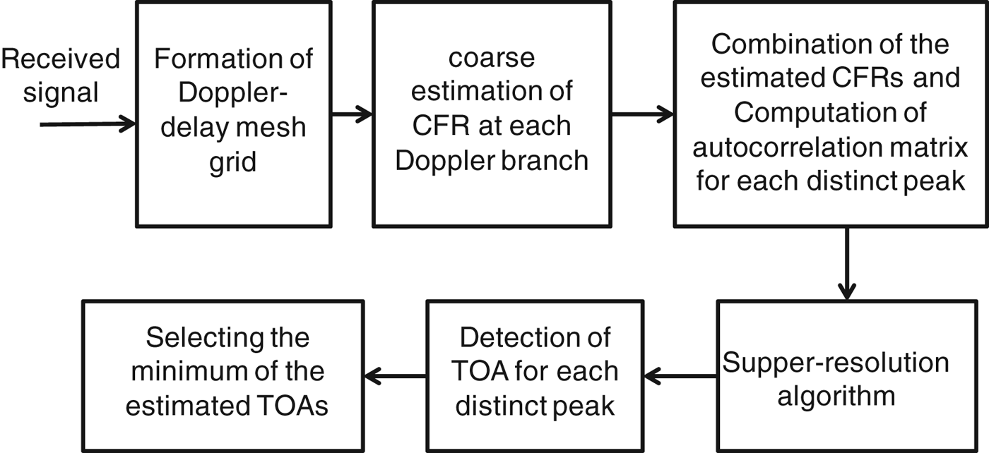
The block diagram of a receiver which employs Doppler combining in super-resolution multipath delay estimation is shown in Figure 1. The delay-Doppler grid of the received signal is first formed at the output of the correlator filter. Next, a rough estimate of the channel frequency response (CFR) is computed for the signal at each Doppler branch (each column of Y in Equation (13)) by spectrum division (Klukas, Reference Klukas1997). The resultant coarse CFRs are combined as defined by Equation (19) to form the channel autocorrelation matrix for each distinct peak (the estimated rough CFRs are located on the columns of ${\bf \hat H}$). Next, singular decomposition (SVD) is applied to the estimated autocorrelation matrix to separate signal and noise subspaces and form the ${\bf P}_{{\bf U}_N} $ matrix. Finally the super-resolution algorithm is used to transform the channel autocorrelation matrix to the super-resolution delay profile, as defined in Equation (26). The estimate of the LOS TOA is then found by detecting the first peak of the delay profile obtained by applying MUSIC to each local maximum of the correlation grid. The final estimate of the TOA will be selected as the minimum of the estimated TOAs for all of the distinct peaks.

Figure 1.

Block diagram of the proposed method.

4.2. When matrix A is singular

Consider the case where the matrix A in Equation (19) is singular with the column rank of M′=2K+1<M. In this case, U_s and U_N have column rank of M′ and L−M′, respectively. Since Equation (24) still holds, multiplying both sides of this equation by ${\bf P}_{{\bf U}_N} $ results in

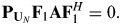(27)$${\bf P}_{{\bf U}_N} {\bf F}_1 {\bf AF}_1^H = 0.$$

By multiplying both sides of Equation (27) by F₁ from the right side and using Equation (18), one obtains

(28)$${\bf P}_{{\bf U}_N} {\bf F}_1 {\bf A} = 0.$$

Moreover, A can be expressed in its singular decomposition form as

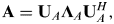(29)$${\bf A} = {\bf U}_A {\bf \Lambda} _A {\bf U}_A^H, $$

where the M×M′ matrix U_A is the vector of the eigenvectors of A and Λ_A is a M′×M′ diagonal matrix with the singular values of A on its diagonal. Substituting Equation (29) into Equation (28) results in

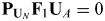(30)$${\bf P}_{{\bf U}_N} {\bf F}_1 {\bf U}_A = 0$$

Since the matrix U_A has the full column rank of M′, Equation (30) implies that ${\bf P}_{{\bf U}_N} $ is orthogonal to M′ independent linear combinations of the columns of F₁. In other words, the column rank of F₁U_A is M′, which is the same as the column rank of the signal space. This fact results in the conclusion that the projection of the matrix F₁U_A is equal to the projection of the signal space (the columns of F₁U_A span the signal space or span{F₁U_A}= span{U_S}), which can be expressed as

(31)$${\bf F}_1 {\bf U}_A {\bf U}_A^H {\bf F}_1^H = {\bf U}_s {\bf U}_s^H. $$

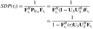
On the other hand, by substituting ${\bf U}_N {\bf U}_N^H = {\bf I} - {\bf U}_S {\bf U}_S^H $ from Equation (22) to the denominator of Equation (26), the SDP function can be rewritten as

(32)$$\eqalign{SDP(\tau _i ) = \displaystyle{1 \over {{\bf F}_{\tau _i} ^H {\bf P}_{{\bf U}_N} {\bf F}_{\tau _i}}} &= \displaystyle{1 \over {{\bf F}_{\tau _i} ^H ({\bf I} - {\bf U}_S {\bf U}_S^H ){\bf F}_{\tau _i}}} \cr \, & = \displaystyle{1 \over {1 - {\bf F}_{\tau _i} ^H (\tau ){\bf U}_S {\bf U}_S^H {\bf F}_{\tau _i}}}} $$

Substituting Equation (31) into Equation (32) results in

(33)$$SDP(\tau _i ) = \displaystyle{1 \over {1 - {\bf F}_{\tau _i} ^H {\bf F}_1 {\bf U}_A {\bf U}_A^H {\bf F}_1^H {\bf F}_{\tau _i}}}. $$

Evaluating the normalized SDP function at different values of the delay while considering that the columns of F are orthonormal results in

(34)$${SDP(\tau _i ) \!=\! \left\{\! {\matrix{ {\displaystyle{1 \over {1 - {\bf F}_{\tau _m} {\bf F}_1^H {\bf U}_A {\bf U}_A^H {\bf F}_1^H {\bf F}_{\tau _m}}} = \displaystyle{1 \over {1 - {\bf U}_A^{(m)} ({\bf U}_A^{(m)} )^H}} \gt 1}& {if\,\,\tau _i = \tau _m \in \{ \tau _0 \,,...,\,\tau _{M - 1} \}} \cr {\displaystyle{1 \over {1 - {\bf F}_{\tau _i} ^H {\bf F}_1 {\bf U}_A {\bf U}_A^H {\bf F}_1^H {\bf F}_{\tau _i}}} = 1} &\hskip-48pt{if\,\,\tau _i \notin \{ \tau _0 \,,...,\,\tau _{M - 1}}}}},\right.$$

where U_A^(m) is the m-th row of U_A. Therefore, the denominator of the SDP function is minimized but non-zero at the delays corresponding to the true multipath delay when A is not full rank and consequently the SDP function is maximized at these points. In other words, in the case where A is rank deficient, the poles of the SDP function are no more located on the unit circle. As the rank of A becomes closer to the number of multipath components, the denominator of the SDP function approaches zero.

In Figure 2, the output of the SDP function is evaluated and plotted for a simulated eight-path channel profile for different values of the rank of the signal autocorrelation matrix.

Figure 2.

(a) CIR of an 8-path channel profile, (b-e) Normalized outputs of the SDP function at signal-to -noise ratios of 20, 10, 5 and 0 dB, respectively.

As can be observed in this figure, the height of the maxima of the function decreases with a decrease in the rank of the autocorrelation matrix. This effect can be so severe that at low SNR values, the peaks due to noise may be even larger than the peaks due to multipath signals, leading to incorrect delay estimations.

It should be noted that the above result was derived based on the assumption that the columns of F were orthogonal to each other. If instead of the DFT matrix, we had chosen F to be the matrix of shifted versions of the ideal autocorrelation function of the PRN code, as is the case in many references (Bouchereau et al., Reference Bouchereau, Brady and Lanzl2001), Equation (34) would not apply. In Figure 3 these two cases are compared for an eight-path simulated channel. It is observed that since the number of diversity branches (N_B=3) is smaller than the number of multipath components (M=7), for the case where the columns of F are the shifted version of the PN correlation function and are not orthogonal (SDP_C), the resulting super-resolution delay profile does not agree with the true simulated channel.

Figure 3.

A comparison between two cases where the columns of F are orthogonal (SDP_D) and non-orthogonal (SDP_C).

5. EXPERIMENTAL RESULTS

In the previous sections, the possibility of taking advantage of frequency shifted copies of the signal in a fast fading channel for the purpose of signal decorrelation in a MUSIC-based delay estimation technique was discussed. In this section, the performance of the proposed estimation technique is assessed by processing a set of real GPS L1 C/A signals captured in a city core, namely downtown Calgary. The environment is an example of an urban canyon with buildings ranging in height from one to over 50 stories. Figure 4 shows the test trajectory (red curve), the sky plot of the constellation at the beginning of the test, the data collection set-up, and the vehicle speed versus time. The part with high buildings is inside the yellow rectangle shown in Figure 4(a). To eliminate the effect of correlated error sources other than multipath, a differential GPS scenario was utilized. Furthermore, an integrated GPS-INS (Inertial Navigation System) was used on the vehicle to obtain continuous reference positions at the one metre level accuracy. These reference positions were employed to assess the positions obtained by the proposed techniques. The computed delay and Doppler shift parameters from the estimated reference data were then passed to a block processing software receiver (GNSRx.ss) and were used to define the centre of the search space.

Figure 4.

(a) Reference trajectory (b) Sky plot of the constellation (c) Vehicle speed (d) Data collection set-up.

A block diagram of the equipment configuration is shown in Figure 5. The GPS signal received by the vehicle-mounted antenna was split into two branches. The first branch was fed into a National Instrument (NI) RF front-end to be amplified, filtered, down-converted and sampled at a rate of 12.5 MHz. The second branch was connected to an integrated GNSS-INS NovAtel SPAN™ system to generate the reference positions. Data from the GNSS portion of the SPAN system was collected by an NI data acquisition board, with a sampling rate of 100 Hz. The antenna and the INS unit were mounted on the vehicle's roof. GPS data was also collected under LOS conditions with another receiver at a base station (reference) for differential processing.

Figure 5.

Data collection architecture.

The raw GPS samples were then processed using GSNRx-ss. In this software receiver, assistance information in the form of broadcast ephemeris, raw data bits and a reference trajectory are utilized to improve tracking sensitivity. The data bits are wiped off using the known data bit information. The signal parameters estimated from the reference trajectory are used to reduce the search space. At each epoch, the reference data, which include position and velocity components, are used to generate the nominal code phase and carrier Doppler that are then passed to the signal processing channels where a grid of correlators is evaluated. Therefore, the output file of the software receiver contains a set of adjustable Doppler-delay correlation grids for each time interval equal to the coherent integration time. The duration of the coherent integration time and the range and resolution of the delay and Doppler values within the correlation grid (the number of Doppler and delay bins) can be set and the output correlation grids are centred on the true LOS delay that is provided by the aiding process. This prior knowledge of the true LOS delay was used to evaluate the performance of the approaches discussed.

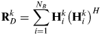
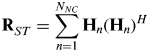
The output correlation grids produced by the software receiver were used for the computation of coarse CFR estimates by applying simple spectrum divisions at each Doppler branch (delay-domain correlation functions corresponding to each Doppler bin) and for each time interval. The outer products of each estimated CFR vector with itself were then computed and averaged depending on each combination approach to form the autocorrelation matrix. In the Doppler combining approach, the self-outer-products of the estimated CFRs on N _B adjacent Doppler branches around each distinct peak were averaged to form the autocorrelation matrix whereas in the spatial-temporal diversity approach, the outer product of the estimated CFRs at the main peak over each N _NC consecutive time snapshots (each equal to the coherent integration time) were averaged to form this matrix. Therefore, the computation of the autocorrelation matrix based on these two techniques can be written as

(35-a)$${\bf R}_D^k = \sum\limits_{i = 1}^{N_B} {{\bf H}_i^k \left( {{\bf H}_i^k} \right)^H} $$

(35-b)$${\bf R}_{ST}^{} = \sum\limits_{n = 1}^{N_{NC}} {{\bf H}_n \left( {{\bf H}_n} \right)^H} $$

where R_D^k is the computed autocorrelation matrix by the Doppler combing technique for the k-th distinct peak, R_ST is the autocorrelation matrix computed by the spatial-temporal diversity technique and H_i^k and H_n are the vectors of estimated CFRs. The ranks of the signal sub-space of R_D^k and R_ST are smaller than or equal to N _B and N _ST, respectively, and the equality holds only if H_i^k (or H_n) are statistically independent (even the independence of only the magnitudes or only the phases of the element of H's suffices).

The MUSIC algorithm was finally applied to the estimated autocorrelation matrices to form the super-resolution delay profiles (SDP) from which the estimates of the LOS times of arrival were obtained. Among all of the peaks in the output SDP that pass a threshold equal to the average magnitude of the SDP, the one that corresponds to the minimum delay is selected as the LOS signal. The difference between the estimated TOAs by the three algorithms discussed above and the one obtained from the SPAN data (the centre of the correlation function), measured in metres, determines the estimated pseudorange error. The values of estimated pseudoranges for all of the visible satellites were finally used to compute the position solution.

It is important to notice that, in practice, during the time interval that it takes to compute every estimate of the autocorrelation matrix from Equation (35-a) or (35-b) which results in a single estimate of the LOS delay, the true value of the delay slightly varies. Therefore, the final estimate is indeed an average of the true delay values within this time period.

Figure 6(a) shows an example of the Doppler-delay correlation function obtained by processing the received signal with PRN 15. In this figure, since the coherent integration time (120 ms) was longer than the coherence time of the channel, three distinct peaks appeared at the correlation surface. These peaks are highlighted in subplot (c). The delay-domain autocorrelation functions corresponding to each peak are shown in subplot (b). Each of these peaks corresponds to a cluster of multipath signals. The speed of the vehicle at the time corresponding to this figure was approximately 9 m/s. For every independent peak, N _B=3 delay-domain correlation functions around the main peak were selected for use in the computation of the CFRs. In Figure 7, the super-resolution delay profiles that correspond to each of the three Doppler branches on peak 1 in Figure 6 and the SDP resulting from their combination using Equation (19) are depicted. As can be seen, the curve representing the combination of Doppler branches includes a clear peak at the centre of the delay range, corresponding to the true LOS time of arrival.

Figure 6.

(a) Example of a Doppler-delay correlation curve with three distinct peaks shown in (c), the delay-domain autocorrelation functions corresponding to each independent peak are shown in (b).

Figure 7.

SDPs corresponding to each of the three Doppler branches on peak 1 in Figure 6 and the resulting SDP from their combination.

Referring to Section 5, the maximum number of effective Doppler branches is $2K + 1 = 2\left\lceil {B_d T} \right\rceil + 1$. Moreover, the relationship between the speed of the receiver and the Doppler spread parameter can be expressed as follows (Rappaport, Reference Rappaport2002):

(36)$$B_d = \displaystyle{v \over \lambda} $$

where v is the speed of the receiver and λ is the wavelength of signal which is almost equal to 0.2 m for L1. It is also important to remember that the coherence time of the channel that limits the effective coherent integration time of the receiver is the inverse of the Doppler spread in Equation (36).

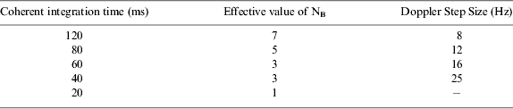
Using Equation (36), for an average speed of 5 m/s, the Doppler spread is around 25 Hz. Considering this approximated value as the Doppler spread of the channel, Table 1 summarises the effective number of Doppler branches and the approximated frequency step size for some different values of coherent integration time.

Table 1.

Effective numbers of Doppler branches for some different values of T.

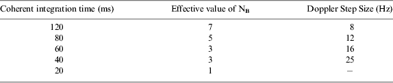
Herein, the range and the resolution of the code delay in the correlation grid were set to ±1 chips (300 m) and 0.03 chips (10 m) respectively, and the range and the resolution of Doppler frequency were set to ±28 Hz and 4 Hz, respectively. Therefore, the size of the correlation grid was 61 by 15. For the first analysis, the coherent integration time of the software receiver was set to T=60 ms. According to Table 1, for this value of coherent integration time, the maximum number of effective Doppler branches is N_B=3. To have comparable results for the Doppler diversity and spatial-temporal diversity techniques, the value of N _NC should be equal to N _B.

Since a slight overestimation of the rank of the signal subspace in the evaluation of Equation (26) does not have a significant effect on the output of the function in practice, N _B and N _NC have been considered as the rank of the signal subspace of R_D^k and R_ST in the computations of Equation (26).

Figure 8 shows the estimated pseudorange errors for all visible PRNs, computed by the Doppler combining-based SDP algorithm (SDP_D), SDP based on spatial-temporal diversity (SDP_ST) and double delta correlator technique.

Figure 8.

Values of estimated pseudorange errors obtained with the three methods.

The correlator spacing parameters for the double delta correlator algorithm was set to 0.1 and 0.2 of a chip (Irsigler and Eissfeller, Reference Irsigler and Eissfeller2003). The coherent integration time for all of the techniques was 60 ms but for the double delta algorithm, the signals on every three successive time snapshots were again coherently averaged for the sake of comparability to the other two combining techniques.

The vehicle entered the high building zone marked by the yellow rectangle in Figure 4(a) at 2000s. Large errors occurred in the estimated pseudoranges for most PRNs as seen in Figure 8. Specifically, the transmitted LOS signals from satellites with lower elevation angels, such as PRN 7, were blocked in some parts of the trajectory. The performance comparisons of the three techniques in terms of pseudorange errors in Figure 8 imply that although exploiting the spatial-temporal diversity could slightly improve the performance of the subspace-based method, this improvement, especially in terms of error bias, is not considerable. For example in Figure 8, large biases can be observed in the values of estimation errors produced by this technique during the time interval 2600–3200 s for PRN 15. The reason is that, in a fast fading situation, the wireless channel observed from the receiver rapidly changes as the antenna moves in the dense multipath environment. For some PRNs such as PRN 15 and 24, even the conventional double delta technique outperforms the temporal diversity-based SDP. On the other hand, taking advantage of only three Doppler branches and combining them in the computation of the signal autocorrelation matrix could result in a noticeable decrease of the estimated biases. Although the resulted improvement is not dramatic for some PRNs, such as 17, a considerable improvement can be observed for PRN 11 and 7. For PRN 28, the estimation errors produced by all the three techniques are very small for the entire test. The reason is that this satellite was located at the zenith during the test time as shown in Figure 4, and this results in a strong LOS signal and insignificant multipath components.

In Figure 9, the RMS values of the computed pseudorange errors for all available PRNs during the yellow area of the test are compared.

Figure 10 shows the corresponding least squares position solution errors using the three methods and in Figure 11, their RMS values are compared.

Figure 9.

Estimated pseudorange error RMS values for the three methods.

Figure 10.

Position solution errors computed by the three algorithms.

Figure 11.

Comparison of the position error RMS values computed by the three methods.

As was expected from the diagrams of the estimated pseudorange errors, the bias values of the position errors computed by the Doppler combining-based method improve as compared to the two other methods. As can be observed in Figure 8, the position errors that correspond to the double delta technique are highly biased in the time duration of 2500–3500 s. The maximum RMS errors produced by the Doppler combining-based method for East and North components are around 20 m (within different PRNs).

In Figures 12 and 13, the pseudorange estimation errors and their RMS values computed by the Doppler combining method for three trade-offs between the receiver's coherent integration time and the number of diversity branches are compared.

Figure 12.

Comparing pseudorange estimation errors for three different values of receiver's coherent integration time.

Figure 13.

RMS values of the pseudorange estimation errors in Figure 12.

The most important point that can be inferred from Figure 13 is that the comparison of the receiver's performance is not the same for all of the satellites. The reason is that the relative velocity between the receiver and each of the satellites and consequently the coherence time of the channel for each satellite is a function of the elevation angle for that satellite. For the satellites with higher elevation angles, such as satellites with PRN numbers of 28 and 26, the coherence time of the channel has a greater value. Therefore they can benefit from longer coherent integration durations at the receiver side. On the other hand for the satellites with the lower elevation angles and lower channel coherence time, long integrations have an adverse effect. For the signals of these satellites, the performance of the receiver can be improved by decreasing the coherent integration and increasing the number of Doppler branches instead. Therefore, depending on the relative velocity between the receiver and a satellite, optimum values for the integration time and the number of diversity branches can be found. For the case of Figure 13, if a fixed integration time is to be considered for all of the satellites, T _c=60 ms seems to be the best choice among the three tested values of the integration time.

It is important to mention here that for those portions of data that corresponded to the sub-urban environment, where the effect of multipath was insignificant, the performance of the three techniques in the sense of pseudorange and positioning errors was similar (as can be observed from the first 500 s in Figures 8 and 10) and the maximum error produced by all of the three techniques was less than 20 m. On the other hand, the computational complexity of a MUSIC-based algorithm is much larger than a classic DLL such as a narrow correlator or a double-delta correlator. This increase in the computational cost is twofold. The first cause of increased complexity is due to applying a large number of correlators to obtain a high-resolution estimate of multipath delays (herein 60 correlators were used for the MUSIC-based technique whereas a narrow correlator only uses three correlators). However, in high sensitivity receivers applying a large bank of correlators is perfectly feasible (SiRFstarIII GSC3e/LP & GSC3f/LP Product Overview). The second cause of complexity is the post correlation matrix manipulations. In the MUSIC algorithm, this complexity mostly results from the singular value decomposition procedure and grows with the third order of the dimension of the autocorrelation matrix (O(N³)) (Trefethen and Bau, Reference Trefethen and Bau1997). Depending on the type of receiver, these computations may require extra software or even hardware to be added to the system. For these reasons, the optimum choice of a signal processing technique is dependent on the application and environment. Specifically, the type of the propagation channel and the expected maximum speed of the mobile device are the main parameters that should be considered.