1 Introduction
The octopus, while not widely praised as a powerful swimmer, performs jet escape manoeuvres with ease and effectiveness, despite its bluff ‘bag-like’ mantle shape in the initial stages of the manoeuvre. Octopodes can be contrasted with squid, whose rigid tunic mantle structures give them a definite advantage in jet propulsion (Gosline & DeMont Reference Gosline and Demont1985). This specialized rigid tunic structure allows the squid to stay streamlined, and does not involve extra expenditure of energy in maintaining mantle length when expelling water for jet propulsion. Octopodes, on the other hand, must spend some metabolic energy maintaining the longitudinal stiffness of its ‘bag-like’ spherical mantle, otherwise radially squeezing of water might cause longitudinal mantle stretching, instead of the intended fluid expulsion to form a jet (Gosline & DeMont Reference Gosline and Demont1985). There is one factor, however, that is overlooked in the literature in giving some fair acknowledgment to the versatility of the ‘bag-like’ shape of the octopus: its large dynamic mantle shape-changing ability, from an initially hyperinflated spherical shape to a streamlined ellipsoidal shape, is shown in this work to aid in added mass energy recovery from the fluid, providing additional thrust and much higher escape velocity than by the jetting alone.
Jet escapes are for avoiding predators, often employed in conjunction with expelling ink to mask the octopus trajectory from the predator. The cycle of normal jet propulsion swimming, that is, mantle hyperinflation, deflation and relaxation, is exaggerated during the more urgent jet escape response and can produce large shape changes in the octopus mantle (Gosline & DeMont Reference Gosline and Demont1985).
The hydrodynamic effect from the shape change is a distinct effect from the jetting alone, as shown by the self-propelled octopus-inspired robot Octobot (Weymouth, Subramaniam & Triantafyllou Reference Weymouth, Subramaniam and Triantafyllou2015). An elastic sheathing is filled with fluid and mounted externally to a rigid streamlined skeleton. When the fluid is released, fluid is expelled to provide jet propulsion forward and also activates shape change of the external elastic sheathing. Image analysis of the shape of the sheath and the speed of the robot shows that the thrust force on the robot is 30 % more than is provided by the jetting alone (Weymouth et al. Reference Weymouth, Subramaniam and Triantafyllou2015). Moslemi & Krueger (Reference Moslemi and Krueger2011) studied pulsed jet propulsion efficiency as a function of Reynolds number, Krieg & Mohseni (Reference Krieg and Mohseni2013) studied non-parallel starting jets to better understand jellyfish and squid jets and Linden & Turner (Reference Linden and Turner2004) discussed optimal vortex ring formation in salps, squid and fish swimming. Gemmell et al. (Reference Gemmell, Costello, Colin, Stewart, Dabiri, Tafti and Priya2013) illuminated the stopping vortex in the deceleration phase of jellyfish swimming as a passive mechanism that gives additional thrust to the jelly. In Gemmell et al. (Reference Gemmell, Costello, Colin, Stewart, Dabiri, Tafti and Priya2013), the stopping vortex mechanism was previously overlooked in contributing to the optimality of the jellyfish jet formation; here, we highlight the distinct contribution and importance of the shape-change mechanism in providing additional escape thrust during the octopus fast jet escape.
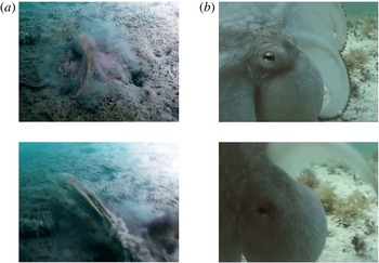
Figure 1(a) shows an example of the shape change employed by octopodes during fast jet escapes (images courtesy of D. J. Schuessler Jr). When the octopus senses danger, it prepares for a fast getaway by taking up extra fluid into its mantle, hyperinflating to an almost spherical mantle shape (top); midway through the jet escape the mantle is much more streamlined in shape (bottom). Figure 1(b) shows a closer view of an octopus preparing to perform a jet escape, showcasing its initially bluff mantle shape (images courtesy of Roger T. Hanlon).
(a) The octopus mantle changes shape drastically from almost spherical (top) to a streamlined shape (bottom) during the course of a jet escape. Images courtesy of D. J. Schuessler Jr. (b) Close-up of an octopus mantle that is nearly spherical in shape, in preparation for a jet escape. Images courtesy of Roger T. Hanlon.

The shape change of octopodes during fast jet escapes allows for added mass energy recovery. Total added mass energy recovery is possible within potential flow for a fixed-shape body; in a viscous flow at least partial energy recovery is still possible, provided large-scale separation does not occur. For a shrinking body it depends on the conditions of body deflation whether energy will be recovered or released to the flow (Weymouth & Triantafyllou Reference Weymouth and Triantafyllou2012): for a deflating body with prescribed kinematics energy is recoverable, provided flow separation is small, while for a ‘melting body’ no energy is recovered. When added mass energy is recovered, conservation of momentum requires that part of the momentum is also transferred back to the body.
Previous work on shape changing bodies demonstrates the concept of added mass energy recovery. Spagnolie & Shelley (Reference Spagnolie and Shelley2009) showed in simulation that for a body changing shape from a circle to an ellipse the sum of body and fluid momenta is conserved. Kanso et al.’s (Reference Kanso, Marsden, Rowley and Melli-Huber2005) work modelled fish swimming as a three-link solid mechanism propelled and steered in potential flow by periodic shape changes, in this case relative rotations between the articulated linkages. Saffman (Reference Saffman1967) studied ways in which manipulating body size, shape and centre of mass would result in added mass energy recovery for net propulsion in an inviscid context. Childress, Spagnolie & Tokieda (Reference Childress, Spagnolie and Tokieda2011) showed that for intermediate Reynolds numbers, recoil locomotion produced by changing both shape and internal mass distribution results in faster swimming speeds as compared with predicted inviscid speeds.
Weymouth & Triantafyllou (Reference Weymouth and Triantafyllou2013) showed that a self-propelled, jetting, shrinking body in simulation, if it is able to avoid massive flow separation, recovers added mass energy to achieve a high escape velocity. In order to focus on the role of the shrinking parameters in the present study, we do not consider the effects of jetting and acceleration. We note that energy recovery is significant, provided that flow separation is prevented; these results are entirely consistent with the results of Weymouth & Triantafyllou (Reference Weymouth and Triantafyllou2013) that include acceleration and jet effects. Weymouth et al. (Reference Weymouth, Subramaniam and Triantafyllou2015) provide an experimental validation that shape change can result in additional thrust due to jet momentum flux, while they introduce a deflation scaling parameter,
 $\unicode[STIX]{x1D70E}^{\ast }$
, based on an analogy with separation prevention through porous suction flow.
In the current work we show through numerical simulations as well as experimental validation that the shrinking speed and Reynolds number are critical parameters, while the specific shape and shrinking amplitude are secondary parameters for successful added mass energy recovery. We also demonstrate that the suction flow analogy is appropriate for shrinking bodies. We adopt the general deflation scaling parameter
 $\unicode[STIX]{x1D70E}^{\ast }=\dot{V}/AU\sqrt{Re}$
from Weymouth et al. (Reference Weymouth, Subramaniam and Triantafyllou2015), where
 $\dot{V}$
is the body volume rate of change,
 $A$
is the frontal area,
 $U$
is the forward velocity and
 $Re$
is the Reynolds number. We define the non-dimensional shrinking parameter here as
 $\unicode[STIX]{x1D70E}^{\ast }={\dot{a}}_{max}/U\sqrt{\mathit{Re }_{0}}$
parameter, where
 ${\dot{a}}_{max}$
is the maximum shrinking speed of the body,
 $U$
is the characteristic forward velocity of the motion and
 $\mathit{Re}_{0}$
is the Reynolds number based on the initial body size, which can predict the degree of success of the added mass energy recovery. Furthermore, the threshold for drag production versus successful thrust production is determined to be
 $\unicode[STIX]{x1D70E}^{\ast }\approx 10$
, and a range of
 $50<\unicode[STIX]{x1D70E}^{\ast }<100$
is shown to result in good recovery performance of 61–82 %.
2 Evaluation of added mass energy recovery performance
2.1 Suction analogy and non-dimensional shrinking parameter
 $\unicode[STIX]{x1D70E}^{\ast }$

Many researchers have investigated separation prevention flow control involving suction through porous walls (Prandtl Reference Prandtl1935; Preston Reference Preston1948; Head Reference Head1959). Prandtl (Reference Prandtl1935) derived the momentum balance equation used to solve for the minimum suction rate needed to prevent incipient separation on a laminar boundary layer. Preston (Reference Preston1948) used similar techniques to show what the threshold suction rate would be on a circle with constant suction applied on the rear half of the circle. Lugt (Reference Lugt1983) explained in layman’s terms that drag reduction techniques such as suction through pores remove fluid particles with low momentum from the boundary layer, thus bringing fresh fluid particles with high momentum to refresh the boundary layer.
Preston’s (Reference Preston1948) equation for the minimum constant suction flow to just avoid laminar separation on a cylinder is
 $v_{1}/U_{0}=3.214\sqrt{\unicode[STIX]{x1D708}/U_{0}D}$
, where
 $v_{1}$
is the suction rate,
 $U_{0}$
is the characteristic flow velocity,
 $\unicode[STIX]{x1D708}$
is the kinematic viscosity and
 $D$
is the diameter of the cylinder. We propose that the form of this suction-based equation can inform our decision of an appropriate non-dimensional parameter to predict and describe the success of added mass energy recovery in shrinking cases. For Preston’s (Reference Preston1948) equation, meeting or exceeding the threshold suction rate prevents boundary layer separation. Analogously, exceeding the threshold shrinking rate prevents massive separation, allowing the wake to reset to follow the instantaneous body size. Since shrinking also imposes a strong normal velocity near the object boundary, we take
 $$\begin{eqnarray}\unicode[STIX]{x1D70E}^{\ast }=\frac{{\dot{a}}_{max}}{U}\sqrt{\mathit{Re }_{0}}\end{eqnarray}$$
to be the shrinking parameter, where
 ${\dot{a}}_{max}$
is the maximum shrinking speed of the body analogous to the suction rate.
2.2 Wake width and added mass recovery ratio
$\unicode[STIX]{x1D702}_{ma}$

Having proposed
 $\unicode[STIX]{x1D70E}^{\ast }$
as the relevant parameter that determines success of the added mass energy recovery, we must also quantify the success of the recovery.
One measure that can indicate whether the energy recovery is successful or not is the wake width. If the width of the wake is larger than the instantaneous body size, we know that momentum is left in the fluid wake and added mass energy recovery is only partial. If the width of the wake is comparable to the instantaneous body size, this is a good indicator that the energy recovery is high.
In addition, we can quantify the recovery through an added mass recovery ratio,
 $$\begin{eqnarray}\unicode[STIX]{x1D702}_{ma}=\frac{\displaystyle \int _{t_{shrink}}F_{x}\,\text{d}t}{U(m_{a,0}-m_{a,f})},\end{eqnarray}$$
where the total impulse of the
 $x$
-direction force
 $F_{x}$
integrated over the entire shrinking time
 $t_{shrink}$
is normalized by the total possible recoverable added mass momentum in the fluid, which is the difference between the initial and final potential flow added masses
 $m_{a,0}-m_{a,f}$
multiplied by the characteristic velocity, in this case the constant towing velocity
 $U$
. The upper limit on this recovery ratio is one, meaning that the entire added mass fluid momentum has been recovered. On the other hand, the recovery ratio can be negative, meaning that there is a net drag on the shrinking body as opposed to net thrust production. The recovery ratio uses the total force in the
 $x$
-direction, including friction and pressure drag; as a consequence, it is different than potential flow would predict, resulting in less recovered energy. When the recovery ratio is zero, there is no net integrated thrust to the body but still some added mass energy has been recovered.
We provide some examples of unsuccessful, moderately high and high energy recovery in shrinking bodies to establish the effect of the principal parameters. In the following three examples the two-dimensional simulated bodies have prescribed kinematics reaching a constant ‘towing’ speed
 $U=1$
from left to right, and experiencing an initial ramped impulsive start from
 $t(U/D)=0$
to
 $t(U/D)=0.1$
, followed immediately by constant towing motion and prescribed body deflation of the instantaneous minor axis length
 $a(t)=a_{0}(1+\unicode[STIX]{x0394}r(t-t_{0}/\unicode[STIX]{x0394}t-\sin (2\unicode[STIX]{x03C0}t-t_{0}/\unicode[STIX]{x0394}t/2\unicode[STIX]{x03C0})))$
, where
 $a_{0}$
is the initial minor axis length,
 $\unicode[STIX]{x0394}r$
is the fraction of shape change (negative for shrinking),
 $t_{0}$
is the time at which shrinking begins and
 $\unicode[STIX]{x0394}t$
is the duration of the shrinking.
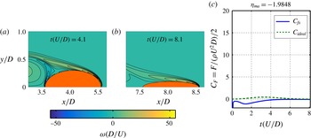
In figure 2, initial Reynolds number
 $\mathit{Re}_{0}=1000$
and maximum shrinking speed
 ${\dot{a}}_{max}=0.1$
give the non-dimensional shrinking parameter to be
 $\unicode[STIX]{x1D70E}^{\ast }=3$
. Figure 2(a) shows the top half of the vorticity wake contours halfway through the shrinking motion and figure 2(b) shows the vorticity contours at the end of the shrinking motion. The wake is clearly massively separated during the shrinking process. Figure 2(c) shows the instantaneous horizontal force on the shrinking body (solid), as well as the potential flow ideal instantaneous horizontal force (dashed), for the entire shrinking motion. Here, the body experiences no thrust production from energy recovery at all, but instead experiences a large drag force, giving a recovery ratio of
 $\unicode[STIX]{x1D702}_{ma}=-2$
. For low
 $\unicode[STIX]{x1D70E}^{\ast }$
we see large wake widths in conjunction with negative
 $\unicode[STIX]{x1D702}_{ma}$
.
Example of non-successful energy recovery for
 $\mathit{Re}_{0}=1000$
and
 ${\dot{a}}_{max}=0.1$
(
 $\unicode[STIX]{x1D70E}^{\ast }=3$
). (a) Vorticity contours halfway through and (b) at end of shrinking motion. (c) The
 $x$
-direction force on body for shrinking times.

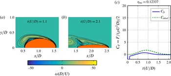
Figure 3 shows an example of moderately high energy recovery (12 %), with initial Reynolds number
 $\mathit{Re}_{0}=1000$
and maximum shrinking speed
 ${\dot{a}}_{max}=0.4$
, giving
 $\unicode[STIX]{x1D70E}^{\ast }=13$
. From figure 3(a,b), the wake follows the instantaneous body size much better than in figure 2, but still exhibits massive separation by the end of the shrinking motion. Looking to figure 3(c), the body experiences thrust production, with a recovery ratio of
 $\unicode[STIX]{x1D702}_{ma}=0.12$
. For this slightly larger
 $\unicode[STIX]{x1D70E}^{\ast }$
we see narrower wake widths and positive
 $\unicode[STIX]{x1D702}_{ma}$
.
Example of moderately high energy recovery for
 $\mathit{Re}_{0}=1000$
and
 ${\dot{a}}_{max}=0.4$
(
 $\unicode[STIX]{x1D70E}^{\ast }=13$
). (a) Vorticity contours halfway through and (b) at end of shrinking motion. (c) The
 $x$
-direction force on body for shrinking times.

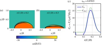
Example of high energy recovery for
 $\mathit{Re}_{0}=1000$
and
 ${\dot{a}}_{max}=4$
(
 $\unicode[STIX]{x1D70E}^{\ast }=127$
). (a) Vorticity contours halfway through and (b) at end of shrinking motion. (c) The
 $x$
-direction force on body for shrinking times.

Lastly, figure 4 shows high energy recovery (87 %), with initial Reynolds number
 $\mathit{Re}_{0}=1000$
and maximum shrinking speed
 ${\dot{a}}_{max}=4$
, giving
 $\unicode[STIX]{x1D70E}^{\ast }=127$
. From figure 4(a,b), the wake follows the instantaneous body size very well throughout the shrinking motion. Figure 4(c) shows that the body experiences thrust very similar to the potential flow ideal, with a recovery ratio of
 $\unicode[STIX]{x1D702}_{ma}=0.87$
. For larger
 $\unicode[STIX]{x1D70E}^{\ast }$
we see narrow wake widths and large positive
 $\unicode[STIX]{x1D702}_{ma}$
.
3 Numerical results
3.1 Numerical set-up
All simulations in this work were performed using a boundary data immersion method (BDIM), as developed by Weymouth & Yue (Reference Weymouth and Yue2011) and improved by Maertens & Weymouth (Reference Maertens and Weymouth2015), with modifications to run the shape change simulations written by the corresponding author. The simulations are fully viscous and can be performed in two and three dimensions.
In all simulations, the body starts with a diameter of
 $D=1$
and experiences a ramped impulsive start from
 $t(U/D)=0$
to
 $t(U/D)=0.1$
. Immediately following this, in all simulations save those testing the influence of the starting timescale in § 3.2, the shrinking profile is superimposed on the constant prescribed forward speed
 $U=1$
. The prescribed radius or minor axis length shrinking kinematics are as follows: instantaneous radius or minor axis length
 $a(t)=a_{0}(1+\unicode[STIX]{x0394}r(t-t_{0}/\unicode[STIX]{x0394}t-\sin (2\unicode[STIX]{x03C0}t-t_{0}/\unicode[STIX]{x0394}t/2\unicode[STIX]{x03C0})))$
and the instantaneous radius/minor axis length shrink speed
 $\text{d}a(t)/\text{d}t=a_{0}\unicode[STIX]{x0394}r/\unicode[STIX]{x0394}t(1-\cos (2\unicode[STIX]{x03C0}t-t_{0}/\unicode[STIX]{x0394}t))$
, where
 $a_{0}$
is the initial radius or minor axis length,
 $\unicode[STIX]{x0394}r$
is the fraction of shape change (negative for shrinking),
 $t_{0}$
is the time at which shrinking begins, and
 $\unicode[STIX]{x0394}t$
is the duration of the shrinking.
A number of three-dimensional simulations were performed to test energy recovery conditions for a sphere shrinking to a prolate spheroid. A Reynolds number range was conducted for
 $\mathit{Re}_{0}=100{-}1100$
and maximum shrink speed range for
 ${\dot{a}}_{max}=0.1{-}4$
.
For two-dimensional simulations, two shape changes were tested: a circle shrinking to a circle and a circle shrinking to an ellipse. Reynolds number range for
 $\mathit{Re}_{0}=100{-}2000$
, maximum shrink speeds
 ${\dot{a}}_{max}=0.1{-}10$
and shrink amplitudes from
 $0.1{-}0.9D$
were also tested.
Convergence tests were performed using simulations of shrinking two- and three-dimensional bodies with identical shrinking kinematics within each convergence testing set. The grid size is geometrically expanding, with the near-body field having a constant, fine grid size
 $h$
.
In two dimensions, a family of three grids of
 $h=1.5\unicode[STIX]{x0394}h_{2D},1.28\unicode[STIX]{x0394}h_{2D},\unicode[STIX]{x0394}h_{2D}$
, where the grid size
 $\unicode[STIX]{x0394}h_{2D}=0.005$
was tested for various Reynolds numbers. Using results from these three grids, an estimate of the convergence rate
 $p$
and true value of the peak force
 $F_{0}$
was calculated from the convergence formula
 $F(h)=F_{0}+ah^{p}$
, where
 $F(h)$
is the peak force value output,
 $a$
is the convergence coefficient and
 $h$
is the grid size. It was found that for two dimensions, based on the convergence requirements that
 $p\geqslant 2$
and the difference between
 $F(h)$
and
 $F_{0}$
is less than
 $2\,\%$
, the shrinking simulations are valid up to a Reynolds number of
 $\mathit{Re}_{0}=2000$
.
In three dimensions, a family of three grids of
 $h=1.6\unicode[STIX]{x0394}h_{3D},1.28\unicode[STIX]{x0394}h_{3D},\unicode[STIX]{x0394}h_{3D}$
, where the grid size
 $\unicode[STIX]{x0394}h_{3D}=0.0101$
was tested for various Reynolds numbers. For the same convergence requirements as stated above, the three-dimensional shrinking simulations are valid up to a Reynolds number of
 $\mathit{Re}_{0}=1100$
.
The BDIM code has also been previously validated for bluff bodies as well as heaving and pitching foils in Maertens & Weymouth (Reference Maertens and Weymouth2015), and has been used in many other works as well, including simulations of shrinking and jetting bodies (Weymouth & Triantafyllou Reference Weymouth and Triantafyllou2013) and retracting foils (Wibawa et al. Reference Wibawa, Steele, Dahl, Rival, Weymouth and Triantafyllou2012).
3.2 Starting timescale
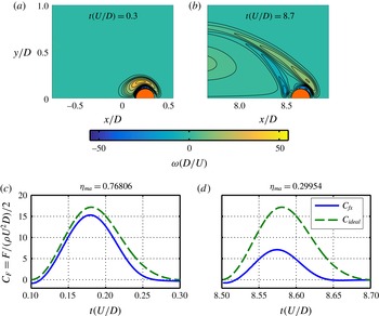
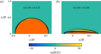
An aspect that influences all of the following results is the specific time when the shrinking motion is triggered. In figure 5, vorticity contours at respective end of shrinking (figure 5
a,b) and corresponding force plots in the shrinking duration (figure 5
c,d) are shown for shrinking circles. The two cases have identical parameters of
 ${\dot{a}}_{max}=4$
,
 $\mathit{Re}_{0}=1000$
and shrink amplitude of
 $0.8D$
, with the key difference that one shrinking motion has started immediately after the impulsive start at time
 $t(U/D)=0.1$
(figure 5
a,c) and the other has started after 8.4 body lengths of travel at
 $t(U/D)=8.5$
, after Kármán street shedding has already occurred.
(a,c) Circle shrinking to a smaller circle right after the impulsive start and (b,d) circle shrinking to a smaller circle after 8.4 body lengths of forward travel. (a,b) Wake vorticity contours at the respective end of shrinking motions, maximum shrink speed and initial Reynolds number held constant at
 ${\dot{a}}_{max}=4$
,
 $\mathit{Re}_{0}=1000$
. (c,d) The
 $x$
-direction force on body for shrinking times.

The wakes of the respective shrinking circles clearly show that the case with the shrinking immediately after the start has boundary layers that closely follow the instantaneous size of the body, while the delayed shrinking case has a large, massively separated wake. The force during shrinking for the first case is also close to the ideal-recovery force (dashed line), while that for the delayed shrinking case is not, giving a recovery ratio of almost 77 % for the first case, versus only 30 % for the delayed deflation case. It should be noted that for the delayed deflation, the flow has separated so that the added mass is significantly different than for attached flow. Owing to these results, all cases following show results for a starting timescale of
 $t(U/D)=0.1$
.
3.3 Maximum shrink speed range
Now we consider numerical simulation results for bodies shrinking from a spherical to prolate spheroidal shape (in three dimensions), or from circular to ellipsoidal shape (in two dimensions) with varying maximum shrink speed. In this set of simulations, all cases were run at
 $\mathit{Re}_{0}=1000$
and shrinking amplitude of
 $0.8D$
on the minor axis. From the force outputs, the recovery ratio
 $\unicode[STIX]{x1D702}_{ma}$
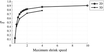
was calculated for each run. From figure 6, for both two- and three-dimensional shrinking bodies, increasing the maximum shrink speed increases the recovery ratio. In addition, the shrinking speed is a critical parameter that can affect whether any energy is recovered at all, since the low speeds 0.1 and 0.2 result in
 $\unicode[STIX]{x1D702}_{ma}<0$
.
Recovery ratio
 $\unicode[STIX]{x1D702}_{ma}$
plotted against maximum shrink speed,
 $\mathit{Re}_{0}=1000$
for two- and three-dimensional simulations.

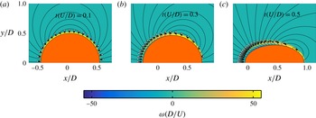
Streamlines of equidistant stream function values, vorticity contours and radially spaced tracer particles, filled lightest to darkest, initially further from the boundary to closer to the boundary layer. Beginning of (a), one-quarter through (b) and halfway through (c) shrinking motion,
 $\mathit{Re}_{0}=1000$
and
 ${\dot{a}}_{max}=1$
.

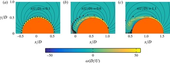
Figures 7 and 8 demonstrate the suitability of considering the shrinking speed as equivalent to suction speed in determining whether the wake separates, as we postulated in § 2.1. Non-dimensional vorticity
 $\unicode[STIX]{x1D714}D/U$
contours, streamlines of equidistant stream function values, the instantaneous body size and position, and radially spaced fluid tracer particles are shown for two simulations. The tracer particles are seeded just outside the boundary layer at non-dimensional time
 $t(U/D)=0.1$
, right at the beginning of the shrinking motion. For figure 7, snapshots are shown at times
 $t(U/D)=0.1,0.3,0.5$
, corresponding to the beginning, one-quarter through and halfway through the complete shrinking motion for a circle shrinking to an ellipse at
 ${\dot{a}}_{max}=1$
. For figure 8, snapshots are shown at times
 $t(U/D)=0.1,0.6,1.1$
, corresponding to the beginning, one-sixteenth through and one-eighth through the complete shrinking motion for a circle shrinking to an ellipse at
 ${\dot{a}}_{max}=0.1$
.
Streamlines of equidistant stream function values, vorticity contours and radially spaced tracer particles, filled lightest to darkest, initially further from the boundary to closer to the boundary layer. Beginning of (a), one-sixteenth through (b) and one-eighth through (c) shrinking motion,
 $\mathit{Re}_{0}=1000$
and
 ${\dot{a}}_{max}=0.1$
.

For the faster shrinking case of figure 7, the tracer particles show that fluid particles from outside the boundary layer, which have high momentum, are brought close to and then inside the boundary layer, injecting increased momentum into the boundary layer, preventing it from separating from the body. Thus, the boundary layer stays close to the body and the wake resets. By contrast, for the slowly shrinking case of figure 8, the fluid particles that are right outside the boundary layer are not drawn in fast enough by the imposed normal velocity of the shrinking body, in order to contribute any momentum addition to the boundary layer. The vorticity contours show the boundary layer to separate from the body, as the wake does not reset to follow the instantaneous body outline.
Hence, we find that the normal velocity imposed by a deflating body can replenish the boundary layer with high-momentum fluid particles to prevent separation, just as the normal velocity imposed by suction flow through pores in a body can replenish the boundary layer with high-momentum fluid particles so that incipient separation is prevented.
3.4 Reynolds number range
Next, results for shrinking recovery ratios
 $\unicode[STIX]{x1D702}_{ma}$
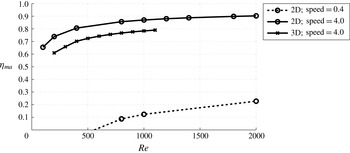
when the Reynolds number is varied are shown in figure 9, for bodies shrinking from spheres to prolate spheroids (in three dimensions) and from circles to ellipses (in two dimensions). All cases in this simulation set were run with shrinking amplitude of
 $0.8D$
on the minor axis.
Recovery ratio
 $\unicode[STIX]{x1D702}_{ma}$
plotted against Re,
 ${\dot{a}}_{max}=0.4$
and
 ${\dot{a}}_{max}=4.0$
for two-dimensional simulations and
 ${\dot{a}}_{max}=4.0$
for three-dimensional simulations.

For all two- and three-dimensional results,
 $\unicode[STIX]{x1D702}_{ma}$
increases with increasing
 $\mathit{Re}_{0}$
, consistent with the physical interpretation that the lower the Reynolds number, the more fluid momentum is diffused out of the boundary layer, impeding the added mass energy recovery. For the two- and three-dimensional results run at a fast shrink speed of
 ${\dot{a}}_{max}=4.0$
, even for low Reynolds number all recovery ratios
 $\unicode[STIX]{x1D702}_{ma}>0$
, whereas for the two-dimensional results run at slow shrink speed
 ${\dot{a}}_{max}=0.4$
for
 $\mathit{Re}_{0}<500$
,
 $\unicode[STIX]{x1D702}_{ma}<0$
. This shows that the shrink speed is critical and that dependence on Reynolds number is important but less critical than shrink speed, consistent with the definition of the non-dimensional shrinking parameter
 $\unicode[STIX]{x1D70E}^{\ast }={\dot{a}}_{max}/U\sqrt{\mathit{Re }_{0}}$
.
3.5 Shape effects
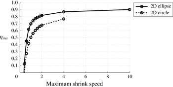
Figure 10 shows recovery ratios against maximum shrinking speed for two different shape changes, from a circle to a smaller diameter circle and from a circle to an ellipse with constant major axis diameter equal to the original circle diameter. All simulations in this set were performed at
 $\mathit{Re}_{0}=1000$
and shrink amplitude
 $0.8D$
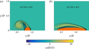
. The results show that for the same shrinking kinematics, shrinking to an ellipse is more effective than shrinking to a circle. Figure 11 shows vorticity contours at the end of shrinking for
 ${\dot{a}}_{max}=1$
for a circle shrinking to both a circle (figure 11
a) and an ellipse (figure 11
b). The circle’s wake is wider than that of the ellipse with identical kinematics, signaling better energy recovery for the ellipse.
Recovery ratio
 $\unicode[STIX]{x1D702}_{ma}$
plotted against maximum shrink speed for circle shrinking to a circle and circle shrinking to an ellipse.

Wake vorticity contours at respective end of shrinking motions for (a) circle shrinking to a smaller circle with 50 % recovery and (b) circle shrinking to an ellipse with 70 % recovery; maximum shrink speed and initial Reynolds number held constant at
 ${\dot{a}}_{max}=1$
,
 $\mathit{Re}_{0}=1000$
.

3.6 Shrink amplitude range
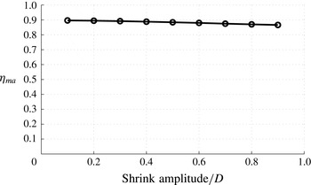
Lastly, we determine the effect of varying the shrinking amplitude. Figure 12 shows the recovery ratios for varying shrinking amplitudes, shown as fractions of the original size
 $D$
, for circles shrinking to ellipses; with
 ${\dot{a}}_{max}=4$
and
 $\mathit{Re}_{0}=1000$
held constant. While there is a decrease in recovery ratio with increasing shrink amplitude, the effect is less than a 5 % difference within the range from 10 % to 90 % shrink amplitude, covering nearly the entire possible range of shrinking amplitude.
Recovery ratio
 $\unicode[STIX]{x1D702}_{ma}$
plotted against shrink amplitude,
 $\mathit{Re}_{0}=1000$
,
 ${\dot{a}}_{max}=4.0$
for two-dimensional simulations.

Although the effect of shrinking amplitude is relatively small, we can explain the decrease of recovery ratio by looking at the near-body vorticity contours. Figure 13 shows the vorticity contours at the end of shrinking for a circle shrinking to an ellipse for 10 % shrinking amplitude (figure 13
a) and 90 % shrinking amplitude (figure 13
b); maximum shrinking speed and initial Reynolds number are held constant at
 ${\dot{a}}_{max}=4$
,
 $\mathit{Re}_{0}=1000$
. As seen, the boundary layer for the larger amplitude is significantly thicker, reducing momentum (and energy) recovery by the body.
Comparison of vorticity contours at the end of two-dimensional shrinking for a circle shrinking to ellipse, and for (a)
 $10\,\%$
and (b)
 $90\,\%$
shrink amplitude; maximum shrink speed and initial Reynolds number held constant at
 ${\dot{a}}_{max}=4$
,
 $\mathit{Re}_{0}=1000$
.

4 Experimental results
4.1 Experimental set-up
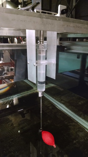
We also validated the energy recovery and wake resetting behaviour experimentally with a deflating and shape-changing body, filled with air and controlled by a linear-actuated 140 cc syringe. The experimental set-up is shown in figure 14. The shape-changing body (‘muscle’) is connected to a thin aluminum hollow tube, which is connected to an actuated air reservoir and allows for air to transfer in and out of the muscle without creating a large disturbance wake. The air reservoir plunger is directly mounted to a Copley Controls STA2504 linear motor, while the reservoir piston is mounted rigidly to the carriage. Optical triggers were set up so that soon after the carriage’s impulsive start, the body deflation begins and continues while the body is towed at constant speed. For flow visualization, the horizontal laser plane is set at half-depth of the shape-changing body, in order to capture the wake at the most representative planar cut through the three-dimensional shape.
Experimental set-up of a deflating body, with air reservoir volume control actuated by a linear motor.

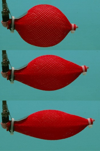
Figure 15 shows the side view of the shape-changing body used, in its fully inflated state (top), partially deflated (middle) and fully deflated (bottom). As in the simulations, the minor axes shrink as the body is deflated; but, due to the design of the body used, the major axis is simultaneously elongated. Nonetheless, the simple construction and repeatable performance of the shape changing body makes this experimental design attractive.
Shape-changing body used in experiments fully inflated (top), partially deflated (middle) and fully deflated (bottom).

4.2 Elongated shape change simulations
First we confirmed that the deflating body’s shape change with simultaneous minor axes shrinking and major axis elongation results in the same overall behaviour as seen in the previous simulations, where the major axis remained constant as the minor axis shrank.
Numerical simulations were performed with this new elongating shape change at
 $\mathit{Re}_{0}=1000$
and three different maximum shrink speeds of
 ${\dot{a}}_{max}=0.1,0.4,4$
(respectively
 $\unicode[STIX]{x1D70E}^{\ast }=3,13,32$
). The elongation of the major axis follows the inverse of the kinematics of the shrinking, with the minor axis shrinking to
 $0.5D$
and the major axis elongating to
 $2D$
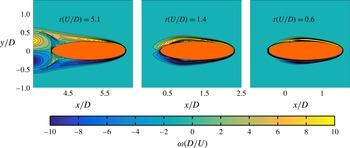
. Figure 16 shows the vorticity contours at the end of respective shrinking motions. The wake massively separates for the slowest shrink speed (left) and resets to follow the instantaneous body size for the faster shrink speeds (middle and right). Thus, the general wake resetting behaviour is the same for the experimental shape changing body as for the previous numerical results.
Elongating shape change simulation vorticity contours at end of respective shrinking motions, for
 $\mathit{Re}_{0}=1000$
and maximum shrink speeds
 ${\dot{a}}_{max}=0.1,0.4,4$
(respectively
 $\unicode[STIX]{x1D70E}^{\ast }=3,13,32$
).

4.3 Particle image velocimetry experimental wake visualizations
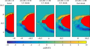
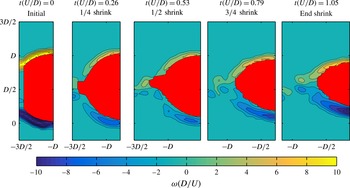
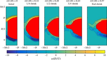
Particle image velocimetry (PIV) results obtained within the half-depth plane of the shape-changing body validate the results of the previous simulations. Figures 17–19 show the experimental near-body vorticity contours of the aft half of the body, from the beginning of the shrinking motion to the end of the shrinking motion, in one-quarter intervals through the shrink motion. Image processing of the raw camera images provide estimates of the shrinking motion duration, instantaneous body shape in the laser plane and shrinking kinematics, since the shape change of the body is not a simple analytic shape change.
Vorticity contours of the near-body wake region of the shape-changing body from experimental PIV data. Snapshots show the wake at one-quarter intervals throughout the shrinking motion. Here
 $\unicode[STIX]{x1D70E}^{\ast }=5$
and the wake is massively separated.

Vorticity contours of near-body wake region of shape changing body, from experimental PIV data. Snapshots show wake at one-quarter intervals throughout shrinking motion. Here
 $\unicode[STIX]{x1D70E}^{\ast }=19$
and the wake successfully resets, with the streamlines following the instantaneous body outline.

Vorticity contours of near-body wake region of shape changing body, from experimental PIV data. Snapshots show wake at one-quarter intervals throughout shrinking motion. Here
 $\unicode[STIX]{x1D70E}^{\ast }=33$
and the wake successfully resets, following the instantaneous body width.

Figure 17 shows the vorticity contours from PIV results, for the shape-changing body at
 $\unicode[STIX]{x1D70E}^{\ast }=5$
. The contours show that the wake is massively separated, consistent with unsuccessful energy recovery. Comparing figure 17 with
 $\unicode[STIX]{x1D70E}^{\ast }=5$
with the left snapshot in figure 16 with
 $\unicode[STIX]{x1D70E}^{\ast }=3$
, we see excellent agreement between the numerical and experimental results.
For figure 18,
 $\unicode[STIX]{x1D70E}^{\ast }=19$
. The experimental vorticity contours here show that the wake resets with the instantaneous body shape, consistent with successful energy recovery. Comparing figure 18 with
 $\unicode[STIX]{x1D70E}^{\ast }=19$
with the middle snapshot in figure 16 with
 $\unicode[STIX]{x1D70E}^{\ast }=13$
, we again see excellent agreement between the numerical and experimental results.
For figure 19,
 $\unicode[STIX]{x1D70E}^{\ast }=33$
. Again the experimental vorticity contours show that the wake resets with the instantaneous body shape, consistent with successful energy recovery. The numerical elongated shape change results show that the
 $\unicode[STIX]{x1D70E}^{\ast }=32$
case, the right snapshot of figure 16, has a narrower wake than the
 $\unicode[STIX]{x1D70E}^{\ast }=13$
case, the middle snapshot of figure 16. We would expect from this numerical results trend that the boundary layers of figure 19 with
 $\unicode[STIX]{x1D70E}^{\ast }=33$
would be thinner than that of figure 18 with
 $\unicode[STIX]{x1D70E}^{\ast }=19$
. Instead we see that the two experimental wakes are very similar. This is attributed to the limited resolution of the experimental PIV seeding close to the body.
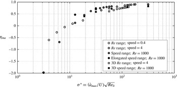
Recovery ratio
 $\unicode[STIX]{x1D702}_{ma}$
plotted against
 $\unicode[STIX]{x1D70E}^{\ast }$
for six simulation sets: two-dimensional simulations of a circle shrinking to an ellipse with (i)
 $\mathit{Re}_{0}=100{-}2000$
with constant shrink speed
 ${\dot{a}}_{max}=0.4$
, (ii)
 $\mathit{Re}_{0}=100{-}2000$
with constant shrink speed
 ${\dot{a}}_{max}=4$
, (iii) shrink speed range
 ${\dot{a}}_{max}=0.1{-}10$
with constant
 $\mathit{Re}_{0}=1000$
, (iv) shrink speed range
 ${\dot{a}}_{max}=0.1{-}4$
for the elongated shape change simulations with constant
 $\mathit{Re}_{0}=1000$
; three-dimensional simulations of a sphere shrinking to a prolate spheroid with (v)
 $\mathit{Re}_{0}=100{-}1100$
with constant shrink speed
 ${\dot{a}}_{max}=4$
and (vi) shrink speed range
 ${\dot{a}}_{max}=0.1{-}4$
with
 $\mathit{Re}_{0}=1000$
held constant.

5 Discussion
Figure 20 shows the compiled numerical results from six of the above numerical data sets, showing the recovery ratio
 $\unicode[STIX]{x1D702}_{ma}$
as the non-dimensional shrinking parameter
 $\unicode[STIX]{x1D70E}^{\ast }$
varies. The sets of data include the following. Two-dimensional simulations of a circle shrinking to an ellipse: (i) varying
 $\mathit{Re}_{0}=100{-}2000$
with shrink speed
 ${\dot{a}}_{max}=0.4$
held constant; (ii) varying
 $\mathit{Re}_{0}=100{-}2000$
with shrink speed
 ${\dot{a}}_{max}=4$
held constant; (iii) varying shrink speed
 ${\dot{a}}_{max}=0.1{-}10$
with
 $\mathit{Re}_{0}=1000$
held constant; and (iv) varying shrink speed
 ${\dot{a}}_{max}=0.1{-}4$
for the elongated shape change simulations with
 $\mathit{Re}_{0}=1000$
held constant. Three-dimensional simulations of a sphere shrinking to a prolate spheroid: (v) varying
 $\mathit{Re}_{0}=100{-}1100$
with shrink speed
 ${\dot{a}}_{max}=4$
held constant and (vi) varying shrink speed
 ${\dot{a}}_{max}=0.1{-}4$
with
 $\mathit{Re}_{0}=1000$
held constant. The prescribed forward speed
 $U=1$
for all simulations.
When plotted against the non-dimensional shrinking parameter
 $\unicode[STIX]{x1D70E}^{\ast }$
, we see that all recovery ratios closely follow the same curve, confirming that
 $\unicode[STIX]{x1D70E}^{\ast }$
is indeed a characteristic parameter of the energy recovery shrinking problem. We also note that our definition here of the non-dimensional shrinking parameter as
 $\unicode[STIX]{x1D70E}^{\ast }={\dot{a}}_{max}/U\sqrt{\mathit{Re }_{0}}$
, where
 ${\dot{a}}_{max}$
is the maximum shrinking speed of the body,
 $U$
is the characteristic forward velocity of the motion and
 $\mathit{Re}_{0}$
is the Reynolds number based on the initial body size, is a more appropriate definition than that introduced previously in Weymouth et al. (Reference Weymouth, Subramaniam and Triantafyllou2015), where the deflation scaling parameter is defined as
 $\unicode[STIX]{x1D70E}^{\ast }=\dot{V}/AU\sqrt{Re}$
, where
 $\dot{V}$
is the body volume rate of change,
 $A$
is the frontal area,
 $U$
is the forward velocity and
 $Re$
is the Reynolds number. For example, in the two-dimensional simulations presented in this work of a circle shrinking to an elongating ellipse, with the major axis elongating as the inverse of the shrinking minor axis of the ellipse, the area is always constant so that the parameter as defined in Weymouth et al. (Reference Weymouth, Subramaniam and Triantafyllou2015) is always zero.
We can extract several overall trends from figure 20 that can be used to exploit the energy and momentum recovery in deflating bodies.
-
(i) The shrinking parameter
$\unicode[STIX]{x1D70E}^{\ast }$
is a good predictor of energy recovery performance and can be used in the design of shrinking and shape-changing robots in the recovery of added mass energy. -
(ii) A threshold value of
$\unicode[STIX]{x1D70E}^{\ast }\approx 10$
is established, to determine whether energy extraction in terms of net thrust is feasible,
$\unicode[STIX]{x1D702}_{ma}>0$
; or not,
$\unicode[STIX]{x1D702}_{ma}<0$
. This is a critical value analogous to the minimum suction rate required to prevent incipient boundary layer separation as described in § 2.1. If this threshold value is exceeded, enough energy recovery for net thrust production is possible. -
(iii) The experimental PIV wake results support the numerical prediction trends based on the
$\unicode[STIX]{x1D70E}^{\ast }$
value. The experimental shape-changing body case with
$\unicode[STIX]{x1D70E}^{\ast }=5$
(figure 17) shows a massively separated wake, consistent with predictions of unsuccessful energy recovery below the threshold value
$\unicode[STIX]{x1D70E}^{\ast }\approx 10$
. The other two experimental shape-changing body cases, with
$\unicode[STIX]{x1D70E}^{\ast }=19,33$
(figures 18 and 19) show wakes consistent with at least partial energy recovery, as predicted for
$\unicode[STIX]{x1D70E}^{\ast }>10$
. -
(iv) A desired performance range of
$50<\unicode[STIX]{x1D70E}^{\ast }<100$
can be established. The performance region
$10<\unicode[STIX]{x1D70E}^{\ast }<30$
is highly transient, with recovery ratio
$\unicode[STIX]{x1D702}_{ma}$
values ranging from 0 to 70 %. Therefore, the less-sensitive region of
$50<\unicode[STIX]{x1D70E}^{\ast }<100$
, with variation of 61–82 % recovery from data points inside the interval, gives a good range of recovery performance. For
$\unicode[STIX]{x1D70E}^{\ast }>100$
there are still recovery gains to be made, but with diminishing returns as compared with merely increasing
$\unicode[STIX]{x1D70E}^{\ast }$
to be beyond the transition range.


We can compare our predictions against some data available on larval squid. Based on experimental measurements of larval squid mantle size and maximum mantle contraction rates during jet escapes available from Thompson & Kier (Reference Thompson and Kier2001) and estimated characteristic swimming velocities of one body length per second, non-dimensional shrinking parameters are estimated to be
 $\unicode[STIX]{x1D70E}^{\ast }\approx 70$
for hatchling squid,
 $\unicode[STIX]{x1D70E}^{\ast }\approx 139$
for young larval squid and
 $\unicode[STIX]{x1D70E}^{\ast }\approx 182$
for larger larval squid. These non-dimensional shrinking parameter estimates are based on squid measurements, because experimental octopus measurements of this kind are scarce; but the shape change present in larval squid show that indeed
 $\unicode[STIX]{x1D70E}^{\ast }$
values obtained from animals agree with the conclusions presented above.
Lastly, we can discuss some aspects of external energy expenditure that must be considered when designing a shrinking machine to take advantage of added mass energy recovery. The fluid-related power is the integral over the exposed body surface (internal and external) of the inner product of the local fluid force (primarily the pressure force) and the local velocity of the body in an inertial frame. This velocity is the vectorial sum of the translational velocity and the local surface-shrinking velocity (relative to the centre of mass of the body), so we can identify two components, one related to the translational and another one related to the shrinking velocity. In a body that is self-propelled, since the latter drives the propulsive jet and the overall manoeuvre, it is expected to be negative when integrated over the total time of the manoeuvre, hence providing the required driving energy. The shrinking energy is expended in accelerating the body, driving the propulsive jet, overcoming the drag force and imparting energy to (or recovering energy from) the fluid in the form of added mass; only the latter energy may be negative since it is recoverable. In self-propelled experiments, the balloon is inflated, storing potential energy in the membrane; this energy is expended for its deflation and is equal to the shrinking energy. Because added mass energy recovery occurs at the later part of the manoeuvre, when the body mass has been reduced as the jet expels mass from the mantle, it has the added beneficial effects of imparting very high final velocity if drag remains small. This is the reason for focusing on the energy recovery aspects of the problem, combined with prevention of separation effects.
6 Conclusions
Octopodes use shape change to recover added mass energy that is first input into the fluid during the onset of a bluff body jet escape manoeuvre. As the octopus releases fluid mass from its mantle to generate thrust, it also deflates and the dynamic shape change allows for recovery of the added mass energy to the energetic advantage of the octopus, since now the simultaneous recovery of the momentum gives a greater burst of escape speed with a lighter mass.
We showed that successful energy recovery is highly dependent on shrinking speed and Reynolds number, with secondary dependence on shape considerations and shrinking amplitude. We confirmed this using numerical results ranging in shrink speed, Reynolds number, shape effects and shrink amplitude, and also validated the results experimentally with a towed and deflating shape-changing body.
The experimental and numerical simulation results when plotted together show that the added mass energy recovery ratio
 $\unicode[STIX]{x1D702}_{ma}$
increases with increasing the non-dimensional shrinking parameter
 $\unicode[STIX]{x1D70E}^{\ast }={\dot{a}}_{max}/U\sqrt{\mathit{Re }_{0}}$
. These results point to a threshold value
 $\unicode[STIX]{x1D70E}^{\ast }\approx 10$
in order to recover energy for net thrust production; below this value not enough energy and momentum are recovered, and, instead, net drag forces develop on the body. The main conclusion is that the shrinking parameter range of
 $50<\unicode[STIX]{x1D70E}^{\ast }<100$
can be targeted in order to achieve significant energy recovery.
Acknowledgements
The authors wish to thank D. J. Schuessler Jr and Roger T. Hanlon for their generous permission to share images from their respective underwater videos of octopodes performing jet escapes. We also wish to thank each anonymous reviewer for their time spent on our paper.