1. Introduction

Studying how evidence is produced and related to theory is an important part of developing and maintaining a discipline. Fields such as psychology, economics, biology, and chemistry have tenured appointments, conferences, societies, and journals (e.g., Psychometrica, Econometrica, Biometrika, Journal of Chemometrics) dedicated to the study and improvement of their methods.

Attention to methods gets increasingly important as matters get more complex and are less well developed. For example, the methods of some parts of economics cry out for attention more so than those of some parts of physics. This is not only because physics is an older discipline and has had time for its methods to mature but also because economics often deals with highly complicated phenomena laden with enormous uncertainties. In such situations, little headway is made without using (and studying, improving, etc.) explicit, typically quantitative, methods for relating evidence to theory.

Whatever else theorizing in linguistics is, it is complex (even if human language is built from just a few relatively simple structural items). Nearly all currently active linguistic projects involve complicated, untamed, and uncharted regions of human language. Moreover, linguistics is a relatively young discipline. Thus, linguistics would seem to be yet another field that would benefit from the incorporation of explicit methods that themselves can be studied, criticized, improved, and so forth. In this article I explore this issue. In section 2, I consider a very basic issue: assessing the size of a given linguistic data set. In section 3, I take an initial step toward explicitly addressing this matter, by suggesting an operationalized characterization of an expression type. In section 4, I consider how this operationalization might help with our assessment. Structurally, the situation is similar to familiar cases involving multivariate data sets, with one exception: the irrelevance of negative associations. This exception, I argue, changes matters considerably. A theorem, proven in the appendix, shows that these negative correlations cannot simply be ignored and that this undesirable phenomenon is quite robust. I conclude in section 5.

The size of one's data set is important; however, my broader goal is to promote greater methodological research in linguistics. Currently, linguists routinely assess large and diverse bodies of evidence almost entirely by informal, holistic, “expert judgments.” Famously, however, in situations vastly less complex than linguistics, expert judgments are much less reliable than they are typically assumed to be (e.g., Dawes Reference Dawes1979; Johnson Reference Johnson and Dreyer2009).

2. Target Issue: Individuating Linguistic Data

I turn now to the basic matter of estimating the size of a linguistic data set. Such a notion is employed, implicitly or explicitly, whenever one judges that a journal article, research project, presentation, and so forth, used “a lot” of data, “not enough” data, a “wide range” of “diverse” data, “more” data than a rival hypothesis is founded on, and so on. Such comments are clearly meant to summarize certain aspects of the evidence and to be part of the overall normative judgment regarding the theory. If “a lot” of data were used, how much was that? More than 15 data points? What were those data points, anyway, and what makes any two of them (if there is more than one) distinct from one another?

The amount of data used in the construction or confirmation of a theory is an utterly fundamental matter across the empirical sciences, especially in those areas where there is great uncertainty and complexity. I will largely take it for granted that it is of similar importance to linguistics to have some (explicit) means for estimating the size of a data set. In general, it is hard to see how progress could be made toward an explicit linguistic methodology if one cannot even say how large one's sample is. (For example, not knowing the size of one's sample severely limits any further analysis or assessment in most experimental designs.)

To begin, let us consider the general type of evidence that mainstream linguists typically employ in actual practice. Simplifying, we can assume the data are linguistic expressions. They are not the psychological data structures realized (under appropriate idealizations, etc.) inside speakers’ heads (e.g., Chomsky Reference Chomsky1986, 25–26). Instead, they are expression types, such as the type of which the physical inscription “the cat is on the mat” is an instance. I will assume that such types can be unproblematically individuated.

In asking how much data were employed by a given linguistic project, a natural first thought would be to just count how many expression types were offered in the project. For example, consider a linguist developing a theory of control, illustrated by sentence 1a.

1. 1a. Sue wants to win.

2. 1b. Sueⁱ wants [PROⁱ to win].

Control structures are noteworthy in that they contain a clause (here, to win) that does not overtly contain a subject. However, in sentence 1a, the subject of this lower clause can only be Sue. This and other such phenomena have led linguists to posit a phonologically null but syntactically and semantically active element, PRO, as the subject of the lower clause (cf. 1b). PRO is “controlled” by Sue, thus mechanically and automatically determining the correct interpretation of the sentence. Suppose that a linguist develops a theory concerning a fragment of human language that includes control structures, which focuses on the phenomenon of “partial control,” illustrated in sentence 2a:

1. 2a. The chair wanted to meet on Tuesday.

2. 2b. Sue wanted to meet on Tuesday.

3. 2c. The chair hoped to meet on Tuesday.

Sentence 2a is noteworthy in that its most natural interpretation is that the chair wanted a group of people, only one of whom is the chair herself, to meet on Tuesday. Thus, the chair only partially determines the subject of the lower clause (i.e., the value of PRO; Landau Reference Landau2000).

The central difficulty with determining how much evidence is used in a theory is that new, redundant data are all too easy to generate. For example, one gathers no new evidence for a theory by adding sentence 2b to a data set containing sentence 2a. Sentences 2a–2b are simply too relevantly similar to count as distinct data points. Of course, sentences 2a–2b have different grammatical properties; for example:

1. 3a. *Crazy old the chair wanted to meet on Tuesday.

2. 3b. Crazy old Sue wanted to meet on Tuesday.

However, it is unlikely that such a difference would be relevant to a theory of control.

What about sentence 2c? The extent to which this expression provides the theory with something new may depend on the nature of the particular theory. As sentences 4 and 5 suggest, sentences 2a and 2c are somewhat different as regards the licensing of possible complement structures:

1. 4a. The chair wanted the committee to meet on Tuesday.

2. 4b. *The chair hoped the committee to meet on Tuesday.

1. 5a. *The chair wanted the committee would meet on Tuesday.

2. 5b. The chair hoped the committee would meet on Tuesday.

However, sentence 6 shows that they behave similarly in other respects, so—depending on the details of the theory at hand—there may be some amount of (relevant) redundancy present.

1. 6a. It was wanted for the committee to meet on Tuesday.

2. 6b. It was hoped for the committee to meet on Tuesday.

These examples show how a pair of expressions may exhibit some degree of redundancy. Importantly, however, redundancy is a holistic affair, potentially involving most or all of the data set. For example, if expressions 7a and 7b are already in the data set, then 7c adds no new information. Similarly, depending on the nature of one's project, expressions 7d and 7e may also be highly redundant with 7a–7b collectively, although not so much with either one individually.

1. 7a. Sue crashed while PRO biking.

2. 7b. Kim wants PRO to be recognized t.

3. 7c. Sue crashed while PRO biking, and Kim wants PRO to be recognized t.

4. 7d. Kim wants PRO to be recognized t while PRO biking.

5. 7e. Kim went unnoticed while PRO wanting PRO to be recognized t.

In sum, an expression may exhibit some degree of redundancy with respect to other elements of a data set. Any such redundancy will always be relative to both a given data set and the particular theory at hand. I will call this phenomenon the “problem of redundancy.” Since linguistic data are used in the construction of a theory as well as its confirmation, what properties of an expression are relevant to an assessment of redundancy—for example, does it license direct objects with controlled complements 4 or tensed clausal complements 5—may not be known a priori. Instead, determining the relevant properties of expressions may be a matter of a “bootstrap” procedure (Glymour Reference Glymour1980) as the theory is developed over time.

The problem of redundancy shows that determining whether one has used “a lot of data” in the construction/confirmation of a linguistic theory is a highly nontrivial matter. If redundancy is not addressed, then there is no difference between any finite data set and a countably infinite one (e.g., augment expression 2a–2b with DP wanted to meet on Tuesday, for every DP). If there is no difference between finite and infinite data sets, then all distinctions regarding the amount of data used collapse.

I suspect that some linguists would see the problem of redundancy as not particularly serious. I also suspect that some linguists feel that as they are constructing or evaluating a theory, they notice such correlations in the behavior of the data and take this into account in an implicit and intuitive manner. In the next two sections, I will attempt to render explicit this purported practice and analyze it.

3. Operationalizing Theoretical Types of Expressions and Their Properties

In linguistic theorizing, we want to relate the evidence of concrete expressions to the theoretical models that produce psychological expressions (e.g., Chomsky Reference Chomsky1986, 25–26). However, we have seen that redundancy threatens to undermine, partially or completely, one of the most basic features of a body of evidence, namely, its size. In this section, I outline a strategy for operationally characterizing the relevant theoretical types of expressions and the relevant properties of these types. Then, in section 4, I consider the problem of redundancy explicitly.

Two key factors motivate our operationalization. First, as sentences 2a–2b and 6 showed, the expressions used as evidence have a great deal of structure, only some of which is relevant to a given project (since we currently have only very partial theories of human language). More generally, a project on control is not likely to be concerned with the highly detailed structures sketched in expressions 8a–8b. Instead, it is more likely to focus on certain schematic aspects of structure that are hypothesized to be those aspects relevant to control, similarly sketched in 8c:

1. 8a. [TP [DP [D′ the chair]] [T′ wanted [VP [CP[TP PRO [T′ to [VP PRO [V′ meet [PP on Tuesday]]]]]]]]]

2. 8b. [TP [DP Sue] [T′ wanted [VP [CP[TP PRO [T′ to [VP PRO [V′ meet [PP on Tuesday]]]]]]]]]

3. 8c. [TP DP [T′ Verb {F ₁, …, F _n} [VP [CP[TP PRO [T′ to [VP PRO [V′]]]]]]]]

The structures in expression 8 are merely illustrative—different theories would posit different structures. However, they show that part of doing linguistics is isolating those structural elements that are/are not relevant to a given project. Because both 2a and 2b have the structure given in expression 8, they count as the same type, and so adding 2b to a data set that contains 2a should not increase the amount of evidence considered.

Of course, we do not have immediate access to the structures in expression 8; determining them is a big part of what linguistics is all about. Here too, linguists often bootstrap into increasingly better theories: the linguist uses current theory to hypothesize some relevant structure thought to be shared by some expressions and thus individuates the data and explores the results so as to arrive at a new (hopefully improved) theory. This new theory is then part of the input that allows the hypothesis of what the relevant types of expressions are that then allows for a new individuation of the data, and so on.

I call theoretical items represented by expression 8c “(theoretical) types.” The difficult task of determining what structure a theoretical type contains belongs mainly to linguists. From the present perspective, however, we can assume that such concrete decisions for particular theories have been made.

The second key fact is that we use expressions like those in sentences 4–6 to explore the nature of theoretical types. In that sense, sentences 4–6 represent what I call “properties” of the types. For example, suppose that the relevant expression types differentiate 2a and 2c—that is, the different kinds of relevant structures that the theory posits are fine-grained enough that one of them applies to 2a and a different one applies to 2c. In such a case, sentence 4 tells us that the type represented with 2a allows direct objects, but the one that 2c represents does not. Similarly, sentence 5 tells us that of the two, only the 2a type allows tensed clauses.

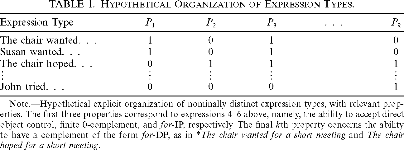
Eventually, in the simplest case, the linguist would posit n theoretical types each examined from the perspective of k properties. The data can then be represented by an matrix, where the ijth element contains a 1 if the ith expression type possesses the jth property, and a 0 otherwise (or by some other coding system if greater discrimination is used). The outcome of this stage of the analysis is represented by table 1: The ith expression type can be operationally defined as the ith row of this matrix, and the jth property can similarly be operationally defined as the jth column. Thus, a theoretical type can also be (operationally) thought of as an equivalence class of expressions all of whose members behave identically across the properties that the linguist has identified as relevant. How reasonable these operationalizations are is largely an empirical matter, to be addressed mainly by linguists.

Table 1Hypothetical Organization of Expression Types.

Expression Type	P 1	P 2	P 3	…	P k
The chair wanted…	1	0	1		0
Susan wanted…	1	0	1		0
The chair hoped…	0	1	1		1
⋮	⋮	⋮	⋮		⋮
John tried…	0	0	0		1

Note Hypothetical explicit organization of nominally distinct expression types, with relevant properties. The first three properties correspond to expressions 4–6 above, namely, the ability to accept direct object control, finite 0-complement, and for-IP, respectively. The final kth property concerns the ability to have a complement of the form for-DP, as in *The chair wanted for a short meeting and The chair hoped for a short meeting.

4. The Problem of Negative Correlations

In section 2, we saw that distinguishing various data points in a linguistic data set is neither trivial nor an all-or-nothing affair. We need to recognize that there can be redundancy in our data sets and that a nominally new addition to a data set may not contribute all that much novel information. Moreover, we saw that the redundancy of an expression may be spread across multiple elements of the data set. We would like to somehow account for this redundancy so as to estimate the true size of our data set.

Fortunately, the issue to which we have reduced our linguistic problem is a familiar one. Intercorrelations in multivariate data sets are a bread-and-butter issue for many fields, and there are numerous statistical techniques for dealing with them. Because we now have explicit representations (from sec. 3) of the relevant aspects of the expressions under study, we can make an assessment of redundancy by considering the amount of “overlap” between the various pairs of theoretical types of expressions. A natural first step would be to consider the correlations between the various types, represented by the n row vectors described above. (In a complete analysis, the k column vectors would be analyzed as well, as there could easily be unwanted redundancy in the relevant properties of the theoretical types. For simplicity's sake, I ignore this matter here.) Such correlations are often the inputs to various techniques for treating redundancy (e.g., Jolliffe Reference Jolliffe2010).

Before turning to these techniques, however, one final empirical consideration must be addressed. The relevant type of redundancy here is only that which corresponds to “positive” correlation. That is, we only care about the extent to which two (operationalized) expression types exhibit the same behavior. In particular, the extent to which they are negatively associated is the same, for the present estimation purposes, as having no association at all. For example, across the right range of properties, pronouns and anaphors are highly negatively correlated. But this high correlation does not suggest that they are redundant; rather, it shows how importantly different they are.

Because negatively correlated theoretical types share no structural redundancy, we might try to disregard them by treating the relevant theoretical types as independent and hence uncorrelated (i.e., having a correlation of zero). At first, this idea seems simple and natural, and it does work in two or three dimensions. Unfortunately, with more than three expressions, there is no guarantee that this strategy will work: the resulting set of correlations often cannot be simultaneously realized. A few remarks may give a sense of why this is so.

When , there are possible correlations. Thus, in fixing these correlations, we have equations of the form (where r is the correlation function), but only n (vectors of) variables to work with. Thus, there is no guarantee that a solution to these equations will always exist.

More can be said. Let , and for any set of n vectors, let be the correlations between each pair of expression types, that is, each pair of k-dimensional vectors. (I assume some canonical ordering of all sets of vectors and of the elements of c.) The “nonnegative variant” of c is the sequence that is just like c except that the negative correlations have been replaced with zeroes. Let us say that c is bad if no set of n vectors could have the correlations of its nonnegative variant. Finally, let . We then have the following robustness theorem, proven in the appendix:

The results just listed apply immediately to the position described at the end of section 3. There I imagined a linguist saying that the problem of redundancy can be dealt with by just noticing and keeping track of the correlations between the data, and accounting for this accordingly, as part of a holistic expert judgment. However, such a strategy simply will not work for a very broad range of data sets and a similarly broad range of measures of association. The reason why has nothing to do with a linguist's expertise; rather, it is a fact about what is mathematically possible.

5. Conclusion

Where does this leave us? We started off by isolating a fundamental issue regarding the evaluation of linguistic theories, counting data. Along the way we helped ourselves to many simplifications, finally ending up with a task vastly simpler than what is routinely performed in linguistic inference. Unfortunately, that simple task is often impossible.

The persistent adherent of informal, holistic expert judgment faces the challenge of demonstrating the accuracy of this method. This may be difficult, as tasks generally do not get easier as they get more complex, and the simple task is not possible. Given the remarkable weakness of such holistic expert judgments in simpler inferential situations, I am not optimistic about these prospects. A more promising strategy, I submit, is to view the present problem as encouragement to follow the other sciences, and begin taking the difficult steps necessary to develop explicit linguistic methods. A first step would be to find a way to estimate the size of a data set, which requires some metric of association to factor out redundancy. I believe common metrics like the correlation are inappropriate for linguistics, which is good since we have just seen that they do not work. But what appropriate metric(s) will work is only one of many questions yet to be addressed.