
1. Introduction
Two-dimensional free-surface capillary flows have been considered by a variety of authors. Due to the assumed incompressibility of the fluid and irrotationality of the flow, most authors make use of complex variable methods. For example, Crapper (Reference Crapper1957) derived an exact solution for periodic capillary waves in infinite depth water (later generalised for finite depth by Kinnersley Reference Kinnersley1976). Unlike periodic wave trains, the model we will consider in this paper has a point where the free surface forcibly separates from a wall.
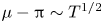
Problems in which the effects of capillarity and gravity are ignored are referred to in the literature as free-streamline problems. In such cases, the constant pressure condition implies that the magnitude of the velocity is constant on the free surface. Consider the cavitating flow past a flat plate, for which there exists a classical Helmholtz–Kirchhoff free-streamline solution. The solution has the property that the curvature at the separation point is unbounded. This does not invalidate the free-streamline solution because the curvature of the free surface does not appear in the boundary conditions. However, it affects the solutions when surface tension is included since there is a term proportional to the curvature of the free surface in the dynamic boundary condition. The effects of surface tension on free-streamline solutions were studied by a variety of authors (Ackerberg Reference Ackerberg1975; Cumberbatch & Norbury Reference Cumberbatch and Norbury1979; Vanden-Broeck Reference Vanden-Broeck1981, Reference Vanden-Broeck1983, Reference Vanden-Broeck1984a). Vanden-Broeck (Reference Vanden-Broeck1981) found a valid asymptotic expansion for small values of the surface tension by allowing a discontinuity in the slope at the separation point. It was found that the angle between the free surface and the solid wall, denoted  $\mu$, varies like
 $\mu -\pi \sim T^{1/2}$, where
 $T$ is the inverse Weber number, given by
 \begin{equation} T = \frac{\sigma}{\rho U^{2} H}. \end{equation}
Here,  $\sigma$ is the surface tension,
 $\rho$ the density of the fluid and
 $U$ and
 $H$ are the reference velocity and length scales, respectively. Hence, as opposed to removing the singularity from the free-streamline solution, the inclusion of surface tension makes the solution more singular by introducing an infinite velocity at the separation point. As well as providing valid asymptotic expansions for
 $T\rightarrow 0$, Vanden-Broeck (Reference Vanden-Broeck1981) also considered the model for large
 $T$. The asymptotic behaviour he found assumed that the
 $T\rightarrow \infty$ solution corresponds to a solution whose free surface was a flat line, extending from the separation point to the flow at infinity. The behaviour described above was also shown via matched asymptotic expansions for the Kirchhoff jet (Vanden-Broeck Reference Vanden-Broeck1984a), and for cavitating flow past a cylinder (Vanden-Broeck Reference Vanden-Broeck1983).
Previous papers considering capillary flows forcibly separating from some solid boundaries have shown that, fixing all the geometry of the model, one finds a single one-parameter branch of solutions for which the flow far away from the solid boundaries is a uniform stream. Starting from a solution with zero surface tension, one finds that as surface tension increases, the profile of the free-surface flattens, and as surface tension is taken to infinity the profile approaches a straight line with zero curvature. This one-parameter branch of solutions was found for the models described above, as well as for the flow under a sluice gate (Tooley & Vanden-Broeck Reference Tooley and Vanden-Broeck2002). A review can be found in Vanden-Broeck (Reference Vanden-Broeck2004).
This paper concerns new limiting configurations for free-surface flows as  $T\rightarrow \infty$. These new solutions all include a point where the flow ‘turns’ at a wall. In this region, high velocities allow the inertial term in Bernoulli's equation to balance the surface tension term. The other components of the free surface are formed of either circles (where the curvature is constant), straight lines (where the curvature is zero) and infinitesimal jets, where large values of the velocity allow for large values of the Bernoulli constant (since the curvature here is also zero). A model exhibiting such solutions is considered, and solved numerically. We discuss the relationship between the velocities and curvatures relative to the inverse Weber number
 $T$ for each limiting configuration. The relations found agree with leading-order balances in the Bernoulli equation. The physical validity of the extreme limiting solutions is certainly doubtful; one would expect viscous effects to play an import role locally at the point where the flow turns near the wall, and more generally in length and velocity scales where surface tension dominates gravity. However, it is still of mathematical interest to explore the solution space of the inviscid model.
2. Formulation
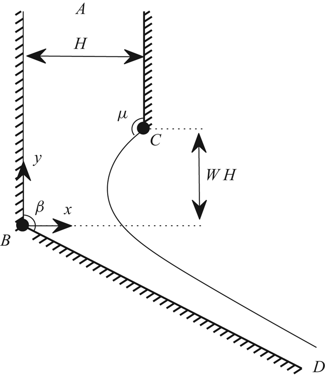
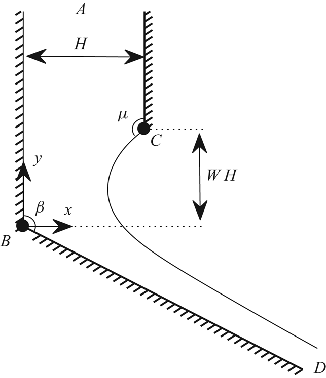
Consider the problem of flow coming in from a two-dimensional channel of width  $H$ with constant velocity
 $U$. One of the walls terminates and forms a free surface, while the other wall meets a second straight wall with an interior angle of
 $\beta$. We choose Cartesian coordinates, where the origin is placed where the two walls meet. We choose
 $x$ to be perpendicular to the channel, and
 $y$ to point in the opposite direction of the uniform stream. We take
 $H$ as the reference length and
 $U$ the reference velocity. The flow separates where the pipe ends with separation angle
 $\mu$. Depending on the value of
 $\beta$, the flow where the two walls meet is either a stagnation point or a point with infinite velocity. The angle at the separation point
 $\mu$ is found as part of the solution. We assume the flow is steady, and the flow configuration is shown in figure 1. We denote by
 $A$ the flow coming in at infinity,
 $B$ the point where the two walls meet,
 $C$ the separation point and
 $D$ the far field. Finally, we denote the non-dimensional distance in the
 $y$-direction between the points
 $B$ and
 $C$ as
 $W$.
Flow configuration in the  $z$-plane.
This model has been considered by a variety of authors with the inclusion of gravity acting in the negative  $y$-direction. When
 $\beta =\pi$, this model was considered with gravity and surface tension by Birkhoff & Carter (Reference Birkhoff and Carter1957), Garabedian (Reference Garabedian1957), Vanden-Broeck (Reference Vanden-Broeck1984a,Reference Vanden-Broeckb, Reference Vanden-Broeck1986), Modi (Reference Modi1985), Couët & Strumolo (Reference Couët and Strumolo1987), Daripa (Reference Daripa2000) and Chandler & Trinh (Reference Chandler and Trinh2018). Due to symmetry, the flow is equivalent to steady rising plane bubbles. When
 $\beta =\pi /2$, Christodoulides & Dias (Reference Christodoulides and Dias2010) and Hocking & Forbes (Reference Hocking and Forbes2010) considered this model with the inclusion of gravity acting in the negative and positive
 $y$-directions, respectively, but no surface tension (in Hocking & Forbes (Reference Hocking and Forbes2010), the passive gas was replaced by a stagnant fluid which was denser than the fluid exiting the pipe). The model in the current paper with both surface tension and gravity for
 $\beta \in [\pi /2,\pi ]$ was considered more recently by Doak & Vanden-Broeck (Reference Doak and Vanden-Broeck2020). None of the above authors considered this geometry with just capillary effects.
We denote the  $x$ and
 $y$ components of the velocity as
 $u$ and
 $v$, respectively. We consider irrotational flow of an incompressible fluid, and hence we can write the velocity field in terms of two harmonic functions, the velocity potential
 $\phi$ and the streamfunction
 $\psi$, defined such that
 \begin{equation} u = \phi_x = \psi_y, \quad v = \phi_y = -\psi_x. \end{equation}
Without loss of generality, we choose  $\phi =0$ at the separation point
 $C$, and
 $\psi =0$ on the streamline
 $ABD$. We denote the velocity potential at
 $B$ as
 $\phi _B$. In this scaling, the streamline
 $ACD$ is given by
 $\psi =1$. We also define the complex potential
 $f=\phi +\textrm {i}\psi$, which is an analytic function of
 $z=x+\textrm {i}y$. The flow domain in the
 $f$-plane is the infinite strip
 $0<\psi <1$. When solving this problem, we will conformally map the flow domain to some auxiliary plane with preferable geometry.
On the free surface (denoted  $x=\eta (y$)), as well as the kinematic boundary condition we also have to satisfy continuity of pressure. This is found by making use of the Bernoulli equation and the Young–Laplace equation. After non-dimensionalisation, this is given by
 \begin{equation} q^{2} + 2 T \kappa = C_B, \quad \text{for} \ x=\eta(y), \end{equation}
where  $q=\lvert \vec {u} \rvert$,
 $\kappa$ is the mean curvature (counted positive when the centre of curvature lies inside the fluid),
 $C_B$ is the Bernoulli constant and
 $T$ is the inverse Weber number, as defined in (1.1). The boundary conditions on
 $\xi$ can then be written as
 \begin{gather} u = 0,\quad \text{for} \ y>0, \ x=0, \end{gather}
 \begin{gather} u = 0,\quad \text{for} \ y\in[W,\infty), \ x=1, \end{gather}
 \begin{gather} u = v\tan\beta,\quad \text{for} \ y<0, \ x=y\tan\beta, \end{gather}
 \begin{gather} q^{2} + 2 T \kappa = C_B, \quad \text{for} \ x=\eta(y). \end{gather}
In the following section, we discuss an exact free-streamline solution, and the numerical method used to solve the flow for non-zero values of  $T$.
3. Free-streamline solution and numerical method
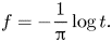
Free-streamline problems were of particular interest in the 19th and early 20th century, since they can often be solved exactly using complex analysis. We find it beneficial to conformally map the flow onto the lower half  $t$-plane via the map
 \begin{equation} f = -\frac{1}{\pi} \log t. \end{equation}
The point  $C$ maps to
 $t=-1$, while the point
 $B$ maps to
 $t=d$, where
 \begin{equation} d = {\rm e}^{-\pi\phi_B}. \end{equation}
The points  $D$ and
 $A$ map to zero and the point at infinity, respectively. The flow in the
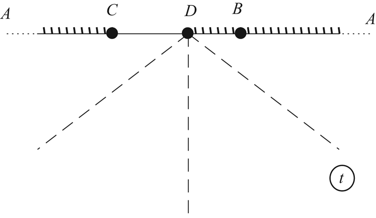
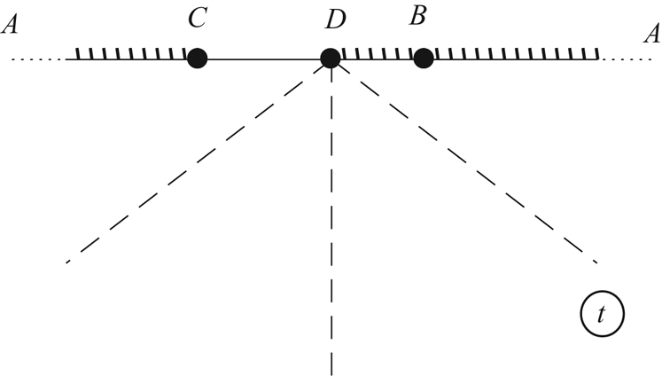
 $t$-plane is shown in figure 2. Following the method proposed by Love (Reference Love1891), one finds that for
 $T=0$, there exists an exact solution given by
 \begin{equation} \log \frac{\textrm{d}z}{\textrm{d}f}(t)= 2 \left(1-\frac{\beta}{\pi} \right) \left[\tanh^{-1}\left(\sqrt{\frac{({d}+1)t}{{d}(t+1)}} \right) - \tanh^{-1}\left( \sqrt{\frac{{d}+1}{{d}}} \right) \right] - \frac{\pi}{2}\textrm{i}. \end{equation}
We find that  $d$ is a free parameter, which has (for any given
 $\beta$) a monotonically increasing dependence on
 $W$. A more in-depth derivation of the above solution is found in Doak & Vanden-Broeck (Reference Doak and Vanden-Broeck2020).
Flow configuration in the  $t$-plane.
When  $T\neq 0$, we need to solve the system numerically. This is done using a boundary integral method. We will not cover the numerical method used in great depth, as many previous authors have deployed such techniques (see Vanden-Broeck (Reference Vanden-Broeck2010) for a review). Applying Cauchy's integral formula on the function
 $\tau -\textrm {i}(\theta +\pi /2)$, where
 \begin{equation} \frac{\textrm{d}f}{\textrm{d}z} = {\rm e}^{\tau-\textrm{i}\theta}, \end{equation}
and where we take the curve of integration to be the union of the real axis and an infinite radius semi-circle in the lower half- $t$-plane, one finds, after some algebra (see Doak & Vanden-Broeck Reference Doak and Vanden-Broeck2020), that for values of
 $\phi _0\in (0,\infty )$ we have
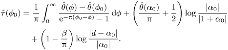 \begin{align} \hat{\tau}(\phi_0) &= \frac{1}{\pi} \int_{0}^{\infty} \frac{\hat{\theta}(\phi) - \hat{\theta}(\phi_0) }{{\rm e}^{-\pi (\phi_0-\phi)} - 1} \, \mathrm{d} \phi + \left(\frac{\hat{\theta}(\alpha_0)}{\pi} + \frac{1}{2}\right) \log \frac{\lvert\alpha_0 \rvert }{\lvert 1+\alpha_0 \rvert} \nonumber\\ &\quad + \left( 1-\frac{\beta}{\pi}\right) \log \frac{\lvert d - \alpha_0 \rvert}{\lvert \alpha_0 \rvert}. \end{align}
Here,  $\hat {\tau }(\phi )$ and
 $\hat {\theta }(\phi )$ refer to values of
 $\tau$ and
 $\theta$ on the free surface, and
 $\alpha _0 = {\rm e}^{-\pi \phi _0}$. The above integral has incorporated the boundary conditions (2.3)–(2.5). Hence, the problem reduces to finding
 $\hat {\tau }$ and
 $\hat {\theta }$ that satisfy (3.5) and the dynamical boundary condition (2.6), which can be written as
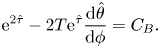 \begin{equation} {\rm e}^{2\hat{\tau}} - 2 T {\rm e}^{\hat\tau} \frac{\textrm{d} \hat{\theta}}{\textrm{d} \phi} = C_B. \end{equation}
We truncate  $\phi$ upstream and downstream to
 $\phi =-\phi _A$ and
 $\phi =\phi _D$, respectively, and we discretise
 $\phi \in [0,\phi _D]$ into
 $N$ equally spaced points. When computing solutions, it must be checked that the solution is invariant to variation in
 $\phi _D$. Taking
 $\hat {\theta }$ at the
 $N$ mesh points as unknowns, we can find values of
 $\hat {\tau }$ in terms of
 $\hat {\theta }$ by satisfying (3.5), where the integral is evaluated numerically using the mid-point rule. One can obtain
 $N-1$ equations by satisfying (3.6) at midpoints (points equally spaced between the
 $N$ mesh points). One also demands a flat far field by setting
 $\hat {\theta }=\pi /2-\beta$ at the final two mesh points. Finally, for a given
 $T$, we fix the value of
 $W$ and allow
 $d$ to vary, where
 $W$ is computed via equation
 \begin{equation} W = \int_{-\phi_A}^{0} y_\phi\lvert_{\psi=1} \, \mathrm{d} \phi - \int_{-\phi_A}^{\phi_B} y_\phi\lvert_{\psi=0} \, \mathrm{d} \phi. \end{equation}
This provides  $N+2$ equations for
 $N+2$ unknowns:
 $\hat {\theta }$ at each mesh point,
 $d$ and
 $C_B$.
Once values of  $\hat {\tau }$ and
 $\hat {\theta }$ have been obtained, one can recover values of
 $\tau$ and
 $\theta$ anywhere in the flow with equations similar to (3.5). One can then obtain streamlines by integrating the identity
 \begin{equation} x_\phi + i y_\phi = {\rm e}^{-\tau+\textrm{i} \theta}, \end{equation}
along lines of constant  $\psi$.
Thus concludes the numerical method used to compute fully nonlinear solutions. For more details, see Doak & Vanden-Broeck (Reference Doak and Vanden-Broeck2020). In the following section, we discuss results.
4. Results
We will focus first on the case of  $\beta =\pi /2$. Fixing the value of
 $W$, we find a one parameter family of solutions. To compute solutions, we can start from the exact solution (3.3) with
 $T=0$. One can then use the method of continuation to find solutions for finite
 $T$. For
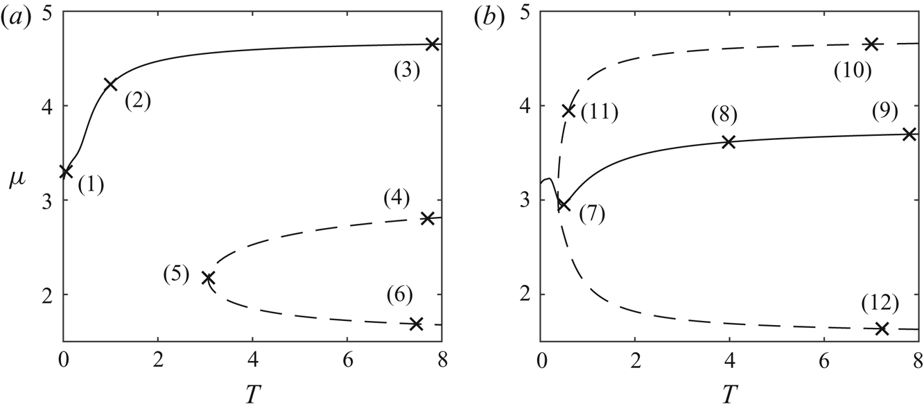
 $W=1$, we find the solution branch one would expect to find; as the value of
 $T$ increases, the separation angle
 $\mu$ monotonically increases from
 $\pi$ (smooth separation at
 $T=0$) to
 $3\pi /2$. As
 $T\rightarrow \infty$, the profile approaches a straight line given by
 $x=-W.$ Denoting the depth of the uniform stream at
 $y\rightarrow \infty$ as
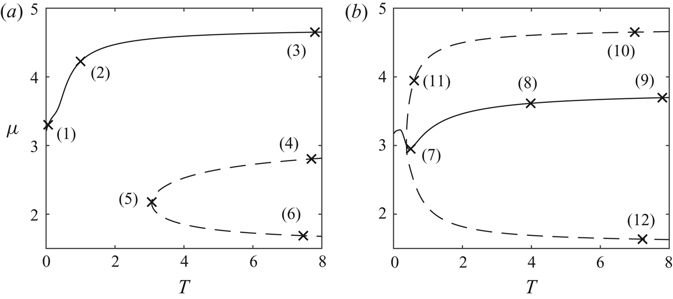
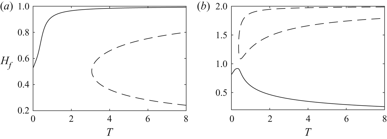
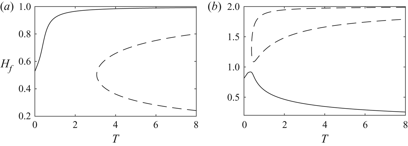
 $H_f$, we plot the branch with a solid curve in
 $(T,\mu )$ and
 $(T,H_f)$ space in figures 3
 $(a)$ and 4
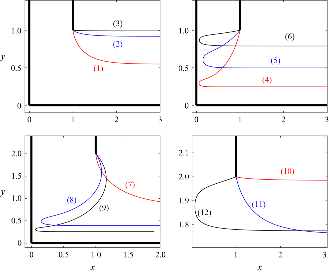
 $(a)$, respectively. Solutions along the branch are shown by the curves (1)–(3) in figure 5.
Panels (a) and (b) are solution branches in  $(T,\mu )$ space for
 $W=1$ and
 $W=2$, respectively. The profiles corresponding to the points (1)–(12) are shown in figure 5.
Panels  $(a)$ and
 $(b)$ are the branches in figure 5 plotted in
 $(T,H_f)$ space for
 $W=1$ and
 $W=2$, respectively.
Solutions corresponding to the points  $(1)$–
 $(12)$ in figure 3.
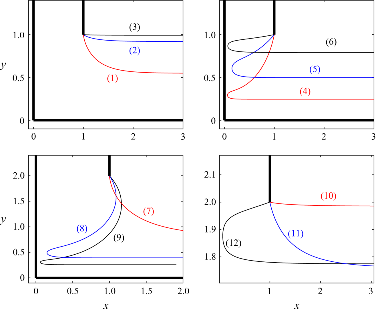
We repeat this computation for  $W=2$. Starting again from the
 $T=0$ solution, we compute the branch for increasing
 $T$. The branch is given by the solid curve in figure 3
 $(b)$, where it is seen that this curve is no longer monotonically increasing. Furthermore, the solution does not approach a flat free surface as
 $T\rightarrow \infty$. Instead, the limiting profile forms a circle whose centre is on the
 $y$-axis, connecting the separation point to the origin. The profile then turns rapidly at the wall, and forms an infinitesimal jet along the
 $x$-axis. One can use the above information to find that the limiting configuration is a circle with centre
 $(0,y_r)$ and a radius
 $R$, where
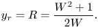 \begin{equation} y_r = R = \frac{W^{2}+1}{2W}. \end{equation}
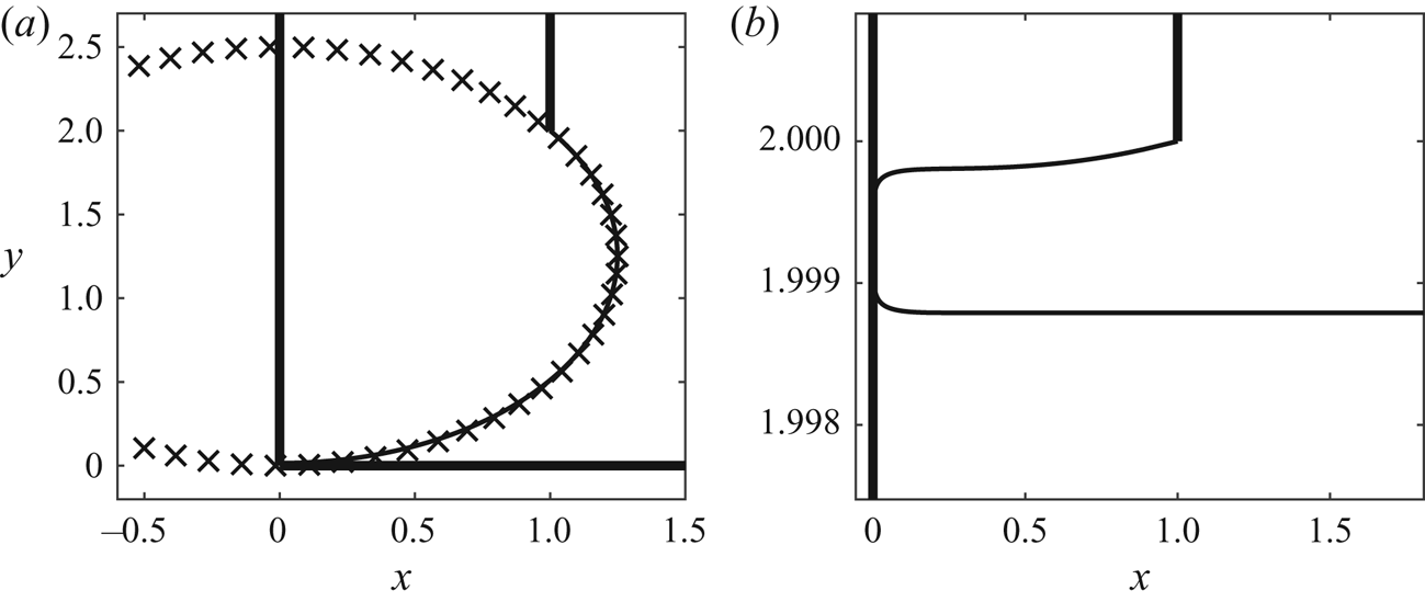
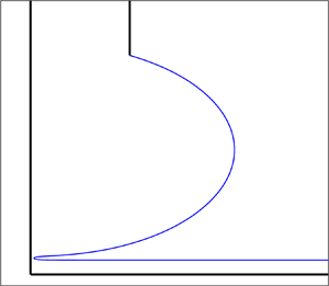
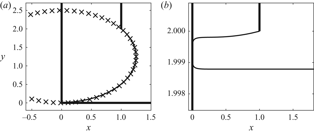
We compare this circle (plotted with crosses) with the solution for  $T=3000$ in figure 6
 $(a)$, where the agreement between the two is found to be very good. Some solutions along the branch for finite
 $T$ are shown by the curves
 $(7)$–
 $(9)$ in figure 5.
Solutions for  $W=2$ and
 $T=3000$, demonstrating the new limiting configurations. Panel (a) shows the solution composed of the arc of a circle, a turning point, and a straight line, while panel (b) shows the solution composed of two straight lines and a turning point. The crosses in panel (a) correspond to a circle with centre (0,R) and radius R, where R is given by equation (4.1).
It is natural to ask what happens along the branch of solutions which contains the purely flat profile for  $T\rightarrow \infty$. Using the method of continuation, this branch is plotted by the dashed curve in figure 3
 $(b)$. It is seen that the solution branch approaches another
 $T\rightarrow \infty$ solution, with
 $\mu =\pi /2$. Some solutions along this branch are shown in figure 5. For large
 $T$, the solution has a flat free surface which goes towards the wall on the
 $y$-axis, forms again this sharp turn and then another flat profile which goes to
 $x\rightarrow \infty$. This solution with
 $T=3000$ is shown in figure 6
 $(b)$. Starting from this large
 $T$ solution, and via continuation in
 $W$, one can find a solution of this type for
 $W=1$. Following the branch, one finds that this branch approaches the other new limiting configuration, which is the profile containing the arc of a circle. This branch is shown in figures 3
 $(a)$ and 4
 $(a)$ by the dashed line.
To help explain these solutions, consider the leading-order balance in the dynamical boundary condition (2.6) for  $T\gg 1$. First, consider the solution characterised by the circle and infinitesimal jet. Along the circle, we have that the curvature is constant, and hence
 $\kappa =O(1)$. Since values of
 $q=O(1)$ here as well, we find that
 $C_B=O(T)$. At the turning point, our numerical results show that here the curvature is negative, and
 $\kappa =O(T)$. These are matched by high values of the velocity, where
 $q=O(T)$. Finally, along the infinitesimal jet,
 $\kappa =0$ and we find that
 $q=O(T)$. This describes how the terms all balance along the three sections of the free surface. For the limiting configuration of two flat lines, one finds that
 $\kappa =0$ along both flat sections. Here,
 $q=O(1)$ and hence
 $C_B=O(1)$. At the turning point, we find the same behaviour as with the turning point for the circle solution, that is
 $q=O(T)$ and
 $K=O(T)$. In both cases, the existence of this additional wall allows a region where high values of negative curvature
 $\kappa =O(T)$ at a turn can be matched with high velocities (due to the thin gap between the wall and the free surface).
We see from figures 3 and 4 that the endpoints of the branches are different for the two values of  $W$. The question arises as to at what value of
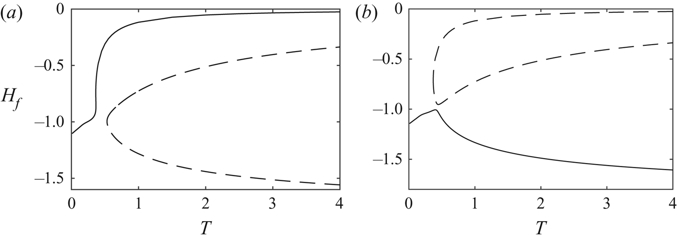
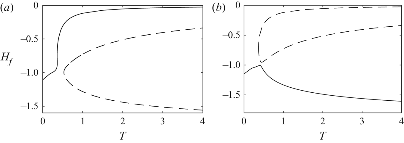
 $W$ does this change occur, and how? In figure 7(a,b), we show the two branches in the
 $(T,H_f)$ for
 $W=1.9$ and
 $W=1.95$, respectively. It can be seen that the endpoints of the two branches have changed at some value of
 $W\,{\in}\,(1.9,1.95)$. We conjecture that, for some critical value of
 $W$, the two branches meet at a bifurcation point.
Solution branches in the  $(T,H_f)$ space for
 $(a)$
 $W=1.9$ and
 $(b)$
 $W=1.95$.
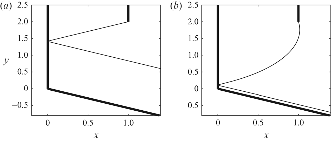
Finally, we note that one can find these new exotic solutions for other values of  $\beta$. We find again two solution branches, connecting four limiting configurations. Two of these are the free-streamline solution and the solution wpproaches
 $\hat {\theta }=\pi /2-\beta$ as
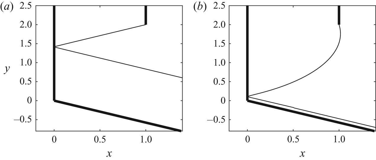
 $T\rightarrow \infty$. The other two limiting configurations are again composed of straight lines and arcs of circles, and are shown figure 8. The solution in figure 8
 $(a)$ is composed of two straight lines and a turning point, while the profile in figure 8
 $(b)$ is composed of the arc of a circle, a turning point, and an infinitesimal jet. They are analogous to the solutions seen in figure 6 for
 $\beta =\pi /2$.
Solutions for large values of  $T$ with
 $\beta =2\pi /3$, demonstrating the new limiting configurations. The solution in panel (a) is composed of two straight lines and a turning point, while the solution in panel (b) is composed of the arc of a circle, a turning point, and an infinitesimal jet.
5. Conclusion
In conclusion, we have found new limiting configurations of capillary free-surface flows. The addition of a boundary which the free-surface can approach and then sharply turn from allows for previously unseen solutions. At the turning point, large values of negative curvature are balanced in Bernoulli's equation with large values of inertia. The limiting configurations are smoothly connected via two one-parameter solution branches. Solutions along these branches with finite  $T$ have been computed, and their behaviour discussed.
Acknowledgments
J.-M.V.-B. was supported in part by EPSRC under grant EP/NO18559/1.
Declaration of interests
The authors report no conflict of interest.