

INTRODUCTION
Benefits of marine reserves for conservation and fisheries management are predicated upon reduced mortality for target organisms inside reserves. Interestingly however, very few studies describe how reserves influence mortality rates (but see Attwood Reference Attwood2003; Willis & Millar Reference Willis and Millar2005; Götz et al. Reference Götz, Kerwath, Attwood and Sauer2008; Taylor & McIlwain Reference Taylor and McIlwain2010). Empirical studies of marine reserves focus on differences in organism density, abundance and size inside versus outside reserves (reviews by Côté et al. Reference Côté, Mosqueira and Reynolds2001; Halpern Reference Halpern2003; Lester et al. Reference Lester, Halpern, Grorud-Colvert, Lubchenco, Ruttenberg, Gaines, Airame and Warner2009), which is sensible because a common objective of conservation is to increase these attributes for depleted populations. Understanding changes in mortality across space in relation to reserve protection is a critical component of evaluating not only the conservation benefit of reserves, but also the contribution of reserves to fisheries management objectives.
Two important fisheries benefits of marine reserves are enhanced by understanding how reserves affect mortality rates of harvested species. The first is the use of populations inside reserves as references for unfished populations (McGilliard et al. Reference McGilliard, Hilborn, MacCall, Punt and Field2010; Wilson et al. Reference Wilson, Prince and Lenihan2010; Babcock & MacCall Reference Babcock and MacCall2011) or for estimating life history parameters used in fishery assessments (Bohnsack Reference Bohnsack1999; MacPherson et al. Reference Macpherson, García-Rubies and Gordoa2000; Taylor & McIlwain Reference Taylor and McIlwain2010; Wilson Reference Wilson2011). A key example of the latter involves estimates of natural mortality (M), which is an essential parameter for many fisheries models (Hilborn & Walters Reference Hilborn and Walters1992), but is difficult to measure, in part because it is confounded by fishing activity in harvested areas outside reserves (Willis & Millar Reference Willis and Millar2005). The second benefit relates to potential increases in fishery yield due to larval export, which results from increased lifetime egg production (LEP) of older, larger and more abundant organisms inside reserves, and the subsequent redistribution of this reproductive output to nearby fished areas (Botsford et al. Reference Botsford, Brumbaugh, Grimes, Kellner, Largier, O'Farrell, Ralston, Soulanille and Wespestad2009). Estimation of reserve-based increases in LEP and fisheries yield is typically based upon individual or population level models that employ estimates of natural and fishing mortality (Beverton & Holt Reference Beverton and Holt1957; Guénette et al. Reference Guénette, Lauck and Clark1998). Consequently, a spatially explicit understanding of how reserves influence mortality is fundamental to understanding if and how reserves can influence LEP and fishery yield.
An additional mechanism by which reserves can benefit fisheries is the net emigration of adults from within reserves to fished areas (spillover). Models of spillover consistently predict that increases in organism abundance and/or biomass inside reserves are lowest near reserve borders because the likelihood of emigration increases near borders, regardless of whether movement is driven by density dependence (Polacheck Reference Polacheck1990; DeMartini Reference DeMartini1993; Sánchez-Lizaso et al. Reference Sánchez-Lizaso, Goñi, Reñones, García-Charton, Galzin, Bayle, Sánchez-Jerez, Pérez-Ruzafa and Ramos2000), diffusion (Hilborn et al. Reference Hilborn, Micheli and De Leo2006; Kellner et al. Reference Kellner, Tetreault, Gaines and Nisbet2007; Walters et al. Reference Walters, Hilborn and Parrish2007), or home ranges that cross reserve borders (Moffitt et al. Reference Moffitt, Botsford, Kaplan and O'Farrell2009). Empirical support for these predictions is mixed (Chapman & Kramer Reference Chapman and Kramer1999; Kaunda-Arara & Rose Reference Kaunda-Arara and Rose2004; Abesamis et al. Reference Abesamis, Russ and Alcala2006; Goñi et al. Reference Goñi, Quetglas and Reñones2006; Harmelin-Vivien et al. Reference Harmelin-Vivien, Le Diréach, Bayle-Sempere, Charbonnel, García-Charton, Ody, Pérez-Ruzafa, Reñones, Sánchez-Jerez and Valle2008), and clear gradients predicted by models are undoubtedly obscured by spatially heterogeneous habitat and ecological processes (García-Charton & Pérez-Ruzafa Reference García-Charton and Pérez-Ruzafa1999). Where present, such gradients might indicate differential mortality inside reserves due to spillover, but no studies have explored changes in mortality as a function of distance from reserve borders. Understanding the magnitude and spatial extent of spillover-mediated fishing mortality inside reserves presents a critical challenge for accurate estimates of biomass or LEP of reserve populations, and for selecting assessment reference sites inside reserves that are not (or are minimally) impacted by spillover.
In this study, we examine how mortality rates for a target organism vary among sites throughout a reserve network and we test two specific predictions: (1) mortality rates are lower inside versus outside reserves, and (2) mortality inside reserves is highest near borders and declines towards reserve centres. To test these hypotheses, we measured mortality rates for California spiny lobster (Panulirus interruptus) on reefs located at varying distances inside and outside borders of three reserves at the Santa Barbara Channel Islands (SBCI) in California, USA. Previous work with P. interruptus at the SBCI reserve network demonstrates robust population increases inside reserves (Kay et al. Reference Kay, Lenihan, Guenther, Wilson, Miller and Shrout2012) and abundance gradients inside reserves that are most likely due to spillover (M. C. Kay, unpublished data 2006–2009). Consequently, this system presents an ideal opportunity to examine how mortality rates vary across space inside and outside of marine reserves. This study is the first to describe spatially explicit and empirical estimates of mortality across multiple reserves in a network.
METHODS
Site selection and sampling
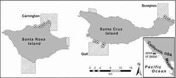
We estimated mortality rates of female California spiny lobster (Panulirus interruptus) populations on 16 reefs inside and outside of three marine reserves at the Santa Barbara Channel Islands (SBCI), California, USA (Fig. 1). General characteristics of the SBCI marine reserve network (CDFG [California Department of Fish and Game] Reference Airarne and Ugoretz2008), as well as the selection process for sites used in this study, are described elsewhere (Kay et al. Reference Kay, Lenihan, Guenther, Wilson, Miller and Shrout2012). Briefly, scientists and commercial lobster fishers worked collaboratively to identify reefs with similar physical, ecological, oceanographic and fishery catch (prior to reserve implementation) characteristics. We sampled six reefs inside or nearby (< 6 km) the Carrington (Santa Rosa Island) and Gull Island (Santa Cruz Island) marine reserves, and we sampled four reefs associated with the Scorpion marine reserve off of Santa Cruz Island (total number of reefs sampled = 6 + 6 + 4 = 16 total). We used GIS (ArcGIS 9.3.1, ESRI) to calculate the distance of the midpoint of each sampling area to the nearest reserve border.
Map showing marine reserves (hashed areas) at Santa Cruz Island and Santa Rosa Island, part of the northern Santa Barbara Channel Islands, in the Southern California Bight (inset). Sampling sites at the Carrington, Gull, and Scorpion reserves are indicated as points within and near each reserve.

We sampled spiny lobster length frequency distributions at each reef using 10–15 replicate lobster traps that were sampled every 1–4 days from August–December 2007 and 2008. Traps were identical to those used in the fishery for P. interruptus at SBCI and are described in detail in Kay et al. Reference Kay, Lenihan, Guenther, Wilson, Miller and Shrout(2012). Traps were deployed in a stratified haphazard array at each reef and were sampled from either commercial fishing vessels or a research vessel equipped with a commercial-grade trap hauler. As each trap was retrieved, we recorded the sex and carapace length (nearest mm using vernier callipers) of all lobsters in the trap. Additionally, lobsters were tagged with an individually numbered T-bar tag (TBA-2 standard, Hallprint Tags, Australia) applied through a thin membrane on the ventral surface between the tail and carapace, such that the ‘T’ portion of the tag was anchored in muscle and persisted through moulting. We minimized stress to lobsters on deck by covering them with wet burlap sacks, placing them in standing seawater, and returning them to the ocean as quickly as possible. After lobsters had been processed, they were returned to the exact location of capture (using GPS coordinates) and released by hand.
Statistical approach
We estimated mortality rates of female lobsters on each reef using a length-based linearized catch curve (LCC) analysis (as described in detail by Sparre & Venema Reference Sparre and Venema1998, Chapter 4). The LCC employs two types of data: (1) length frequency data, as described above, and (2) estimates for parameters of the Von Bertalanffy growth function (VBGF) using:

where Lt is the length of individuals at age t, L∞ is the mean asymptotic length, K is the growth rate and t0 is the theoretical age at which length is zero. We estimated these parameters from lobsters that were tagged and recaptured over a three-year period (2006–2009) at our field sites (Fig. 1). VBGF parameters were estimated using an expression of the VBGF that is explicitly designed for use with tag-recapture data where length at initial tagging, the length at recapture, and time elapsed between tagging and recapture are used to estimate L∞ and K (Quinn & Deriso Reference Quinn and Deriso1999). This can be expressed as:

where ΔLj is the change in length (growth increment) between tagging and recapture for individual lobster j, Lij is the initial length of lobster j at tagging, Δtj is the time elapsed between initial tagging and recapture for individual j, and L∞ and K are free parameters estimated by the model.
Several aspects of recapture data used to estimate L∞ and K warrant mention. (1) t0 is not estimable from tag-recapture data alone and, by convention, we assume t0 = zero. (2) Reliable estimates for L∞ and K were not obtained for male lobsters because annual growth increments for the largest males we tagged and recaptured were as high as the maximum annual values we observed at any size class, and therefore we were not able to reliably estimate L∞ (the mean asymptotic size). Rather than assuming equal growth for both sexes, or forcing a value for male L∞ , we opted for a more conservative approach and proceeded with an analysis that considers growth and mortality for female lobsters only. (3) Recapture data were pooled from all sites in our study. (4) We fitted Eq. (2) to lobsters that were captured within three weeks of the anniversary of their tagging in order to minimize bias that resulted from seasonal and incremental growth over very short time intervals or during time periods that did not include all annual seasons. This required a large number of individual lobsters to be tagged, and the analysis here employed 481 females recaptured from the c. 9756 females tagged. (5) We used data only from lobsters that were tagged and recaptured inside reserves in order to avoid underestimates of K due to differential harvest of fast-growing individuals and underestimates for L∞ due to truncated size structure of fished populations.
Once VBGF parameters were estimated, a LCC was analysed as described by Sparre and Venema (Reference Sparre and Venema1998). The first step was to convert our length frequency size classes (1 mm bins) into age classes. This was accomplished by entering our VBGF parameter estimates from Eq. (2) into the inverse Von Bertalanffy equation:

where AgeL is the age of lobsters at individual size class L (here, 1 mm bins), and t0 , K, and L∞ are as previously described. Next, the proportion of lobsters in each age class in the observed data (namely length frequencies converted to age classes using Eq. 3) was adjusted using the following equation:

where Nadja is the adjusted proportion of lobsters at age a, Na is the proportion of lobsters in age class a from the observed length frequency data (converted to age classes) and Δta is amount of time that a lobster with average growth spends in age class a (estimated directly from results of Eq. 3).
These two steps (Eqs 3 and 4) yield a linear relationship between Nadja (the y-axis variable, hereafter referred to as ln frequency) and each age class (the x-axis variable), to which a least squares linear regression can be fitted:

where Nadja (ln frequency) is the adjusted number of lobsters in each age class a, Xa represents each age class a, Z is the slope of the regression line and b is the y-intercept. The parameter of interest in this regression is Z, whose negative value is the mortality rate. Data for each of our sampling sites (Fig. 1) were plotted separately and Eq. (5) was fitted to data for each site. The age class in which the greatest percentage of lobsters was captured represents age at which animals are fully selected by fishing gear, and Eq. (5) was not fitted to data points to the left of this peak. Finally, in order to measure the effect of marine reserves on mortality rates, Eq. (5) was fitted only to age classes not exposed to fishing pressure prior to reserve implementation in April 2003 (thus age classes above the legal size limit prior to April 2003 were excluded from LCC analyses at all sites).
We characterized uncertainty in our VBGF parameter estimates by fitting Eq. (2) to 1000 bootstrapped subsamples (with replacement) of our tag-recapture data. Similarly, uncertainty in our length frequency data was characterized by bootstrapping (with replacement) 1000 individual subsamples of the observed data. Individual estimates of L∞ and K were then interacted with individual length frequency subsamples (Eq. 3) to produce 1000 unique arrays of age classes. We then applied Eqs (4) and (5) to each of these unique arrays, such that we ultimately attained 1000 estimates of Z (mortality) at each site. The mean (± SD) of these 1000 estimates are reported for each of our 16 sites inside and outside reserves.
Mean estimates of spiny lobster mortality (Z) at our 16 sites were used in linear regression analyses to examine spatial differences in mortality across the Santa Barbara Channel Islands reserve network. To test the hypothesis that reserves decrease mortality for populations within their borders, we specified the following regression model:

where response variable Y is the mortality (Z) we estimated at our sites, α is the intercept (constant), In_reserve is a categorical variable indicating sites inside any reserve, and Scorpion and Carrington are categorical variables for sites associated with the Scorpion and Carrington reserves, with Gull as the omitted category. Coefficient β describes the influence of the In_reserve predictor variable (the location inside versus outside any of the three reserves) on the response variable, coefficients γ and δ account for the average differences in response variables by reserve using Gull as the basis for comparison and ε is the error term (variance not explained by the model).
To test the hypothesis that mean mortality rates at each site change depending upon distance from marine reserve borders, we specified the following model:

where Y is the mortality we estimated at our sites, Distance_in and Distance_out are continuous variables and are vectors of distances of individual trapping sites inside or outside the nearest reserve border, respectively (for sites inside borders, Distance_out values were set to zero, and for sites outside borders, Distance_in values were set to zero), and Gull and Carrington are categorical variables for sites associated with the Gull and Carrington reserves, with Scorpion as the omitted category. Coefficients β1 and β2 describe the influence of Distance_in and Distance_out on the response variable, coefficients φ and δ account for the average differences in response variables by reserve using Scorpion as the basis for comparison, and α and ε are as described above. Regression models were specified to be robust to heterogeneity of variance and were estimated using STATA 9 (StataCorp 2005). Statistical significance was determined at the 0.05 level.
RESULTS
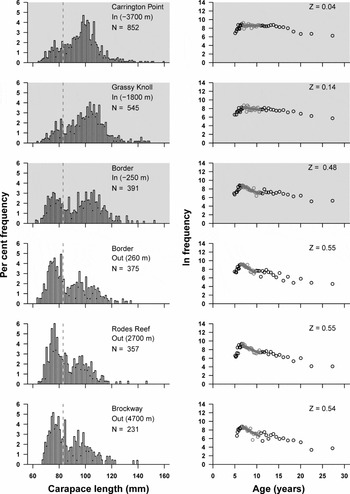
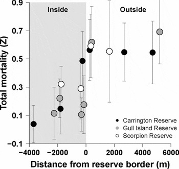
Length frequency data at the innermost Carrington reserve site (Carrington Point, 3700 m from nearest border) showed a clear mode centred at c.100 mm carapace length (Fig. 2). Among all sites within the Carrington reserve, the height of this mode relative to smaller size classes became progressively smaller with proximity to the reserve border. This pattern is reflected in the catch curve mortality estimates at each of these sites, which show a clear relationship between increased mortality and proximity to the border. Specifically, the mortality rates at individual sites ranged from Z = 0.04 at Carrington Point, 0.14 at Grassy Knoll (1800 m inside) and 0.48 at the Border site (250 m inside; Fig. 2). Length frequency data at sites outside the Carrington reserve were comprised of fewer large-sized lobsters than at sites inside the reserve, and corresponding mortality estimates were higher (Z = 0.54–0.55) and far less variable than for sites inside reserves (Fig. 2).
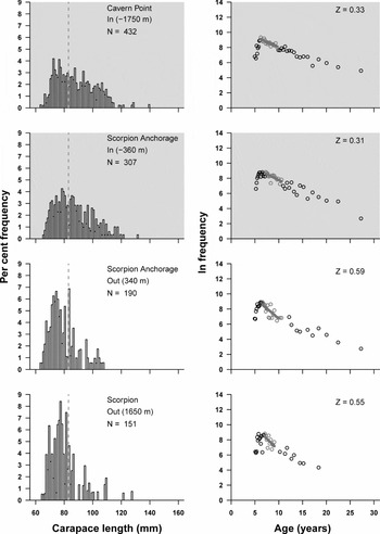
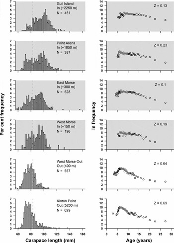
Length frequency distributions (left column of panels) and linearized catch curve (LCC) plots (right column of panels) for female lobsters sampled at sites in or near the Carrington marine reserve. Length frequencies and LCC plots for a single site are adjacent panels, such that data for each sampling site are presented as paired panels in a single row. Sites inside reserves are shaded grey. Also reported in length frequency panels are the distances of sampling sites from the nearest reserve border (negative values for sites inside reserves) and the number of lobsters in each sample. Dashed line represents the minimum legal size limit (82.5 mm). Total mortality (Z) at each site is reported on the LCC panels.

Length frequency data and corresponding mortality estimates for the Scorpion reserve (Fig. 3) indicated important similarities and differences when compared to the Carrington sites. Unlike Carrington, no mode of larger animals was evident in the length frequency data, and mortality estimates for the two sites inside the reserve were both relatively high (Z = 0.33 for Cavern Point, 1750 m inside, and 0.31 for Scorpion Anchorage, 360 m inside). However, as with the Carrington sites, sites outside the reserve had higher mortality than sites inside the reserve (Z = 0.59 at Scorpion Anchorage, 340 m outside, and 0.55 at Scorpion Far, 1650 m outside).

At the Gull Island reserve, length frequency data at the innermost site (Gull Island, 2250 m inside reserve) showed a mode centred on c. 103 mm (Fig. 4) that was absent at Punta Arena (1850 m inside), East Morse (300 m inside) and West Morse (150 m inside). Interestingly, catch curve mortality estimates among these sites are highest at Punta Arena (Z = 0.23), similar at Gull Island and East Morse (Z = 0.10), and intermediate at West Morse Point (Z = 0.19). Mortality estimates at sites outside reserves were much higher than inside (Z = 0.64 and 0.69 at Morse Point Out, 400 m outside border, and Kinton Point, 5200 m outside border).

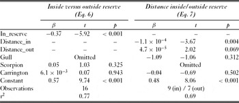
The mean mortality rate among the nine sites inside all three reserves was 0.22 (± 0.05 SE), but was 0.59 (± 0.02 SE) for the seven sites outside reserves, and the difference was significant (Fig. 5, Table 1). The coefficient value of β = −0.37 for Eq. (6) indicates that the average effect of reserves was a Z reduction of 0.37. The relationship between mortality rate and distance from nearest reserve border was significant for sites inside reserves, and the coefficient value β1 = −0.0001 (Table 1) in Eq. (7) indicates a marginal effect of reserves, such that Z was reduced by 0.0001 for every metre moved from reserve borders towards reserve centres. A notable exception to the general pattern was relatively low mortality measured at the East Morse and West Morse sites immediately inside the Gull reserve border.
Mean total mortality (Z), estimated with LCC, and the distance from nearest marine reserve border for of each of the 16 sites associated with the Carrington, Gull, and Scorpion reserves. Grey shading indicates sites inside reserves. Error bars are 95% confidence intervals. Mean values for each site shown in this figure were used in subsequent regression analyses.

Linear regression tests of the effects of location inside versus outside reserves and distance from reserve borders (predictor variables) on mortality (response variable) across sampling sites. Values reported for predictor variables include the coefficient (β), the t-statistic (t) and the p value.

DISCUSSION
This is the first empirical study in which mortality rates for a fished species were examined across multiple reserves and as a function of distance from reserve borders. Drastically reduced mortality for female lobsters inside reserves across the SBCI network (Fig. 5, Table 1) indicates that these reserves are an effective conservation tool. This reduced mortality is likely the primary driver of the increased numbers and sizes of lobsters observed by Kay et al. Reference Kay, Lenihan, Guenther, Wilson, Miller and Shrout(2012) at the same sites, and linking the two results is important because perceived reserve effects can be confounded by high spatiotemporal variability in marine systems (García-Charton & Pérez-Ruzafa Reference García-Charton and Pérez-Ruzafa1999; Willis et al. Reference Willis, Millar, Babcock and Tolimieri2003). Our prediction that mortality inside reserves should be influenced by distance from borders was confirmed statistically, but the only individual reserve to demonstrate the pattern clearly was Carrington. This trend may strengthen over time as lobster abundance and mean size continues to increase inside the relatively young SBCI reserves (for example Kelly et al. Reference Kelly, Scott, MacDiarmid and Babcock2000; Shears et al. Reference Shears, Grace, Usmar, Kerr and Babcock2006).
In general, site-specific mortality rates for female lobsters were far less variable outside reserves than inside reserves. Our spatially explicit regression model (Eq. 7) accounted for 69% of the total variance (Table 1) of Z estimates among sites, and most variability was observed inside reserves. This suggests that spillover-mediated fishing mortality is one of multiple factors that cause highly variable mortality inside reserves.
Variable mortality within reserves has important implications for the use of reserves as fishery management tools. If some fraction of total mortality (Z) experienced by populations immediately inside borders is due to spillover-mediated fishing mortality (F), then sites inside reserves that are used to estimate natural mortality (M) should be located near the interior of reserves. The distance inside reserves at which total mortality is representative of M and not (or very minimally) impacted by F is a function of the relative scales of organism movement and reserve size (Kaunda-Arara & Rose Reference Kaunda-Arara and Rose2004; Moffitt et al. Reference Moffitt, Botsford, Kaplan and O'Farrell2009). Tagging studies at the SBCI indicate that nearly 80% of tagged lobsters are recaptured within 2 km of their initial tagging site, and the distance moved is not time-dependent (Kay et al. Reference Kay, Lenihan, Miller, Barsky, Airame and Ugoretz2008). This scale of movement is smaller than the width (measured as the linear along-shore distance between borders) of the Carrington (c. 7.7 km), Gull (c. 4.7 km of shoreline, but c. 7.7 km maximum width because the reserve extends further west just offshore; see Fig. 1), and Scorpion (c. 4.1 km) reserves. Given these relative spatial scales, sites located c. 2 km or further inside reserve borders in this study provide reasonable estimates of M for female lobsters. Among the five sites not immediately inside reserve borders, the mean estimate of Z was 0.17 (± 0.05 SE). This estimate, and the overall mean estimate from sites within reserves (0.22 ± 0.05 SE), is similar to M values estimated for other temperate spiny lobster species (Pollock Reference Pollock1981; Groenveld Reference Groenveld2000; Caputi et al. Reference Caputi, Melville-Smith, de Lestang, How, Thomson, Stephenson, Wright and Donohue2008; Haist et al. Reference Haist, Breen and Starr2009).
Variable total mortality inside reserves might reflect actual differences in M, but additional explanations include dynamic ecological processes between sites/reserves or biases in the models we used. For example, relatively low mortality at the Gull border sites (East and West Morse Point; Figs 4 and 5), as compared to the Scorpion and Carrington border sites, may be due to two important physical features. First, sampling at the West and East Morse sites occurred near a prominent rocky reef (Morse Point) that provides high relief habitat, reaches the sea surface even at high tide c. 150 m offshore, and has a history (pre-reserve) of high catches. Furthermore, this feature extends offshore within the reserve for many miles as a deepwater (c. 50 m deep) ridge, and the local ecological knowledge (LEK; Hartley & Robertson Reference Hartley and Robertson2009) of fisher collaborators indicates that this might serve as a seasonal migration corridor. These physical attributes may reduce along-shore movement across the nearest reserve border and into fished areas, which would lower mortality rates of populations at this site. This effect is suggested by lower mortality at East Morse (interior side of Morse Point) than at West Morse (border side of Morse Point), even though the two sites are separated by only c.150 m (Fig. 5). No such feature is present at the Carrington border, and relatively high Z estimates at both Scorpion sites may be due in part to the narrow width (and thus higher emigration) of that reserve. The second physical difference is that the Gull reserve is south-facing, whereas the Scorpion and Carrington reserves face north. This is important because large winter storm swells during the fishing season transmit higher energy to nearshore reefs on the north-facing side of the Channel Islands, and such storm events trigger large-scale lobster movements that likely increase emigration rates.
An alternative explanation for lower total mortality measured at the Gull border is that, while M and per caput emigration rates might be the same at all border sites, larger size classes show a behavioural preference for the type of habitat at Gull Border relative to Carrington and Scorpion border sites. This explanation is feasible because commercial and recreational fishers’ LEK suggests that lobsters are often distributed heterogeneously, based on demography (sex and/or size class) and habitat. This is supported by previous observations (M. C. Kay, unpublished data 2008) which recorded a significant relationship between lobster size and the density of lobster dens across the same sites in this study, and the common observation that small size classes use surfgrass (Phyllospadix spp.) as a preferred habitat (Engle Reference Engle1979). Indeed, these ecological relationships might explain why perceived mortality rates at Punta Arena (Z = 0.23) were high relative to those at Gull Island (Z = 0.13), even though the sites are similar distances from reserve borders. Specifically, a large area at the Punta Arena site is a shallow and low-relief surfgrass meadow, whereas Gull Island has greater structural complexity, higher density of lobster dens (M. C. Kay, unpublished data 2008) and a reputation for historically high fishery catches characterized by large lobsters. Consequently, it is possible that the disparity in Z estimates for these two sites is an artefact of bottom-up ecological differences that select for different size classes of lobsters and therefore bias estimates of our length-based model. Although this conclusion is speculative, it underscores the importance of interpreting fisheries models in the local ecological context to which they are applied, and it demonstrates the prudence of estimating M from multiple sites near reserve centres.
Low variability in mortality rates (Z) among sites outside reserves, as compared to Z inside reserves, may be due to spatially heterogeneous fishing effort that is allocated in proportion to the abundance of target organisms. This behaviour is predicted by the ideal free distribution (Abrahams & Healy Reference Abrahams and Healy1990) and is documented under certain circumstances from at least one other crustacean fishery (Swain & Wade 1993). Adherence to the ideal free distribution is variable within and among fisheries (Abernethy et al. Reference Abernethy, Allison, Molloy and Côté2007), but it is possible that mortality imposed through heterogeneous fishing effort at our sites may have masked the high natural variability in Z that was apparent inside reserves.
This study quantifies the conservation value of a reserve network for reducing mortality to female P. interruptus. The fact that we detected a significant mortality-distance relationship inside reserves, but mortality was highly variable, demonstrates the need for further empirical study to elucidate spatially explicit mortality patterns inside and outside marine reserves. Ideally, future studies will explore the generality of distance-mortality relationships inside reserves and relate these to known movement rates for multiple species. Increased mortality for populations immediately inside reserve borders indicates a fundamental trade-off between spillover benefits to adjacent fisheries and benefits to fisheries derived from increased LEP or reserve-based assessments. The inherent trade-off is that spillover effectively connects reserve populations with fished areas, such that some level of fishing mortality is exerted on reserve populations, but LEP and the accuracy of estimates for M are maximized when fishing mortality is absent inside reserves.
CONCLUSION
Linking estimates of mortality inside reserves to rates of spillover is an important frontier in marine reserve research, because doing so allows direct comparison of the trade-offs between spillover (and consequent increased mortality inside reserves) and LEP and the reliability of reserve-based assessments. We demonstrate here that variable mortality inside reserves does not preclude use of reserves in estimating M, but care must be taken in selecting reference sites, especially when ecological heterogeneity can bias models.
ACKNOWLEDGEMENTS
We thank our fishery partners who assisted with trapping of spiny lobsters, especially C. Miller, S. Shrout and S. Davis. Field assistance was provided by S. Horwath, S. Rathbone and J. Heard. D. Hall (Hallprint Tags, Australia) provided expedited support. Funding for this work was provided by California Ocean Protection Council/California Coastal Conservancy research award 07-021 to M. C. Kay, J. R. Wilson and H. S. Lenihan, and California Sea Grant award NA10OAR4170060 to H. S. Lenihan, J. R. Wilson and M. C. Kay. J. R. Wilson was further supported by grants awarded to the Sustainable Fisheries Group (UCSB) from the Waitt Foundation and The Nature Conservancy. The manuscript was improved by the comments of T. Ben-Horin, T. Willis and three anonymous reviewers.