2. MINIMUM CONTRAST ESTIMATION

Let {X_t} be a Gaussian stationary process with mean zero, autocovariance function R(·), and spectral density g(λ), λ ∈ [−π,π] . We consider fitting some parametric family

of spectral densities to the true spectral density g(λ) by minimizing a (distance) criterion. To describe the first-order asymptotics of our estimator it is not strictly necessary to assume Gaussianity of the process. Nevertheless, for discussing the higher order asymptotics, the assumption of Gaussianity seems essential for two reasons: first, because our estimator and many other estimators, e.g., Yule–Walker and Whittle estimators, are not generally first-order asymptotically efficient for non-Gaussian cases; and second because the higher order asymptotics for non-Gaussian cases are tremendously complicated. Hence we will assume Gaussianity of the process throughout this paper.

Initially, we will also make the following assumption.

Assumption 1.

(ii) The fitted model f_θ(λ) belongs to

and is four times continuously differentiable with respect to θ.

Taniguchi (1987) introduces the criterion

which measures the nearness of f_θ to g. Expressions (E1)–(E4), which follow, are typical examples.

This criterion is equivalent to the quasi-Gaussian ML type criterion

(Hosoya and Taniguchi, 1982; Taniguchi and Kakizawa, 2000).

This is given in Taniguchi (1979 and 1981).

defines a family of criterions indexed by α.

This is an α-entropy criterion for a Gaussian process (see Albrecht, 1983).

Let us define a pseudo-true value of θ by

To estimate θ(g), we need to estimate g(λ) because g(λ) is unknown. For this purpose we will use a nonparametric window type estimator, whose window functions W(·), W_n(·), and w(·) satisfy the following assumptions.

Assumption 2.

(i) The function

can be expanded as

It is easy to see that the Parzen window and Daniell window satisfy (i)–(iii) (see Hannan, 1970, p. 279). Throughout this paper we use the following nonparametric spectral estimator:

where

. It is known that

(e.g., Hannan, 1970; Brillinger, 1981). The associated minimum contrast estimator of θ(g) is defined by a value of θ that satisfies the equation

Under certain additional assumptions, Taniguchi (1987) gives the asymptotic distribution of

and shows that

is first-order asymptotically efficient if {X_t} is Gaussian and if g = f_θ; i.e.,

where

.

We will motivate the estimator further by demonstrating the advantages claimed in the introduction over likelihood and QML methods, but first we will show the necessity of using a kernel instead of the raw periodogram.

If D(f_θ,g) is a linear integral functional of g(λ), then we can use the periodogram

in place of

, i.e.,

. The Whittle estimator or quasi-Gaussian ML type criterion is a typical example. If D(f_θ,g) is a nonlinear integral functional of g(λ), however, then

in probability, and the raw periodogram should not be used. This inconsistency can be understood from the following example. Consider

Because

, are asymptotically independent g(λ_j)χ₂²/2 variables (e.g., Brillinger, 1981, p. 126), we can see

Therefore, A_n [nrarr ] 0 (n → ∞), which implies

The point is that if h(.) is a nonlinear function, then in general

and we need to use

instead of the raw periodogram

.

Advantages of

over quasi-Gaussian ML type estimators are as follows: (a1) When the spectral density is contaminated by a sharp peak, the functional defined by K(x) = log{(1 − α) + αx} − α log x, (α ∈ (0,1)), is robust with respect to peak; (a2) for a given g, if we choose K(·) appropriately, then this estimation method provides explicit, noniterative, and asymptotically efficient estimators for various spectral parametrizations.

To see (a1), for

(Assumption 1), let

, which are the functionals of the quasi-Gaussian ML and α-entropy estimators, respectively. For arbitrary given ε > 0 and δ > 0, define

where r > 1 and the interval [λ₀ − δ,λ₀ + ε + δ] is chosen so that [λ₀ − δ, λ₀ + ε + δ] ⊂ [0,π]. Then we can construct a smooth version

satisfying that

on Ω and [λ₀,λ₀ + ε] and that

is differentiable with respect to λ ∈ [0,π] . On the interval [λ₀ + ε, λ₀ + ε + δ] , we can define

where

(see Billingsley, 1968, p. 41). We can make an analogous

. For λ ∈ [−π,0] , we define

. Because

, we can choose positive numbers L₁ and L₂ so that L₁ ≤ f (λ)/g(λ) ≤ L₂. From the definition we have

In (2.6) and (2.7), first taking δ → 0, second taking ε > 0 sufficiently small, we observe that (2.6) tends to infinitely large and that (2.7) tends to zero, which implies that D_α(f,g) is robust with respect to the peak contaminated spectral density

but that D_ML(f,g) is not.

It may be noted that Kakizawa, Shumway, and Taniguchi (1998) discuss discriminating between earthquakes and mining explosions by use of the criterion based on D_α(f,g). They report that the criterion works well for these seismic data.

To illustrate point (a2), suppose that {X_t} is generated by the following MA(p) model:

where {u_t} is a sequence of i.i.d. N(0,σ²) random variables. In this case we use

where

. The criterion (2.8) is a dual version of the criterion (E1) (i.e., K(x) = log x⁻¹ + x). Then, noting that

is independent of θ, we can see that the minimum contrast estimator

based on (2.8) is given by

where

(p × p matrix) and

. In the actual computation, we evaluate the integrals by their Riemann sums. The estimator

is noniterative and asymptotically efficient.

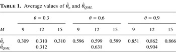
For the particular case with p = 1, σ² = 1, and n = 300, we calculated

and the quasi-Gaussian ML estimator

which minimizes

with respect to θ, and we iterated this procedure 1,000 times for three different values θ = 0.3, 0.6, 0.9. Here we used Daniell's window to calculate

with M = 9, 12, and 15. Table 1 shows the averaged values of

θ_n and

.

Average values of

From this table we observe that the minimum contrast estimation procedure works well, even in comparison with quasi-Gaussian ML type estimators.

Point (a2) can also be understood if we consider the exponential type spectral density

(Bloomfield, 1973), and if we take K(x) = (log x)², then the noniterative asymptotically efficient estimator

for θ = (θ¹,…,θ^p)′ is given by

Of course we could calculate

for the preceding θ by using Newton–Raphson's iterative method, but in this case, we would still need a consistent initial estimator.

Because the function K(·) is only assumed to satisfy (iii) of Assumption 1, we can construct infinitely many first-order asymptotically efficient estimators, and it is desirable to distinguish between them. To analyze their difference we discuss higher order asymptotics of

and related quantities in the next section.

3. HIGHER ORDER ASYMPTOTICS OF FUNDAMENTAL QUANTITIES

In view of the general asymptotic theory, higher order asymptotics of

are most easily described in terms of those of

where a(λ) is a continuous function and A(·) is a four times continuously differentiable function. Expanding

at g(λ) we obtain

where

and A^(j)(x) = (∂^j/∂x^j)A(x). The following lemma asserts that the third term β₃ is negligible in the second-order sense. We have placed the proofs of the lemmas of this paper in the Appendix.

LEMMA 1. Under Assumptions 1 and 2,

The other terms, β₁ and β₂, are evaluated as follows.

LEMMA 2. Under Assumptions 1 and 2,

LEMMA 3. Under Assumptions 1 and 2,

Combining the preceding results gives the following theorem.

THEOREM 1. Under Assumptions 1 and 2, it holds that

It is also easy to show the following lemma.

LEMMA 4. Under Assumptions 1 and 2,

4. HIGHER ORDER ASYMPTOTIC THEORY FOR MINIMUM CONTRAST ESTIMATORS

In this section we discuss higher order asymptotic efficiency of the minimum contrast estimator

defined by (2.5).

Throughout this section we assume g = f_θ, so that efficiency is discussed when the model is correctly specified. This is important for a meaningful comparison between minimum contrast estimators and (quasi-) ML methods. The robustness properties are therefore not analyzed further than in Section 2. We also will not pursue the validity of the Edgeworth expansion and stochastic expansion for

because it is very technical and essentially parallel to the discussion given in Section 4.2 of Taniguchi and Kakizawa (2000). Hence we omit the proofs of Lemmas 5 and 6, and Theorems 2 and 3 (i.e., we only give the proofs of Lemmas 1–3 and 7 in the Appendix).

LEMMA 5. Let ξ be an arbitrary positive number and let C be a compact subset of Θ. Then, there exists a statistic

that solves (2.5) such that for some d > 0,

uniformly for θ ∈ C.

Expanding the right-hand side of

with respect to

at θ, we have

where ∂_i = ∂/∂θⁱ. Here we use the Einstein summation convention: summation is automatically taken over all possible values without an explicit Σ sign for those indices that appear twice in the same term, once as a subscript and once as a superscript.

Because θ is the pseudo-true value defined in equation (2.2) it holds that ∂_i D(f_θ,g) = 0, and we have

Write

It follows from (4.4) that

Solving (4.5) with respect to

we obtain the following lemma (cf. Taniguchi and Kakizawa, 2000, Sec. 4.2).

LEMMA 6. Denote by I^ij the (i,j)th element of the inverse matrix of {I_ij}. Then,

To describe the higher order asymptotics of

we need the following quantities:

The next lemma uses these to give explicit expressions for fundamental quantities.

LEMMA 7. Let the parametric family

contain the true spectral density g. Then under g = f_θ,

Denote by

the (i,j)th element of the inverse matrix of

and let κ = K⁽³⁾(1)/K⁽²⁾(1). From Lemmas 6 and 7 the asymptotic moments (cumulants) of

are evaluated as follows:

The Jth order cumulants of

satisfy

for each J ≥ 3.

From the general Edgeworth expansion formula (e.g., Taniguchi, 1991, p. 14; Taniguchi and Kakizawa, 2000, p. 169) we get the following theorem.

THEOREM 2.

where

,

the multivariate normal distribution, and multivariate Hermite polynomials:

To discuss higher order efficiency and establish unified higher order results we need to restrict the class of estimators to second-order unbiased or second-order median unbiased (cf. Ghosh, 1994; Akahira, 1986; Taniguchi, 1991; Taniguchi and Kakizawa, 2000; Xiao and Phillips, 1998). We restrict the class to second-order median unbiased estimators which are defined as follows. If a consistent estimator

of θ satisfies

then

is said to be second-order asymptotically median unbiased (AMU) (e.g., Akahira, 1986, Sec. 2.5). We denote by

the class of all the second-order asymptotically median unbiased (AMU) estimators of θ. We discuss the second-order asymptotic efficiency of

in the class

.

It can be seen that

is not second-order AMU (cf. Taniguchi, 1991, p. 25). Thus we modify

as follows:

(cf. Akahira, 1986, Sec. 2.5). Then we have the following theorem.

THEOREM 3.

(i) The estimator

is second-order AMU.

(ii) The second-order asymptotic distribution of

is

Remark 1. The bias correction term does not affect the first-order asymptotics. The bias-corrected estimator

therefore inherits the first-order robustness of

, and we can focus on the efficiency of

in the class

without having to trade off efficiency against robustness.

Recall the definition of c^ijk(θ) given by (4.9). It can be seen that if κ = −4, then Edg₂(x,−4) becomes the second-order efficient bound distribution. Also it may be noted that if θ is scalar (and we can drop the indices) (4.14) becomes

where

. Summarizing we have the following result.

THEOREM 4. The bias-corrected minimum contrast estimator

is second-order asymptotically efficient in the class of second-order AMU

, if and only if the contrast function K(·) is such that

The preceding results are remarkable.

Remark 2. In the usual parametric estimation theory it is known that “first-order efficiency implies second-order efficiency” (e.g., Ghosh, 1994, p. 57). However, our results claim that, in semiparametric estimation, “first-order efficiency does not imply second-order efficiency in general.” This is a sharp contrast between the usual parametric estimation and semiparametric estimation and is due to the fact that we may use a wide variety of “nonlinear functionals D of g.”

Remark 3. Theorem 4 can be employed to check whether the estimator based on K(·) leads to a second-order efficient estimator. We give four examples of K(·), which all lead to a first-order asymptotically efficient estimator. Here we examine whether they satisfy the condition κ = K⁽³⁾(1)/K⁽²⁾(1) = −4 or not and are therefore second-order efficient or not. Let us denote

Then it is easily seen that

Remark 4. The bias-corrected Whittle estimator is second-order asymptotically efficient in the class of second-order AMU

, which is not surprising given that the contrast function K₁(·) is of Whittle type. The Whittle estimator can be sensitive, however, and in view of the robustness properties (i) and (ii) of the introduction, it seems important to elucidate the second-order asymptotics of our minimum contrast estimators generally.