


The use of antimicrobials in human and veterinary medicine has brought tremendous benefits to both humans and animals over the past century, benefits increasingly threatened by the development and progression of antimicrobial resistance (AMR). While AMR can be naturally-occurring, antimicrobial use (AMU) in animal agriculture, human medicine, and other settings is a major selection pressure for acquired AMR. AMR and the resulting reduction in drug effectiveness threaten both public and animal health (Marshall and Levy, Reference Marshall and Levy2011; Oliver et al., Reference Oliver, Murinda and Jayarao2011). It is thus vital that antimicrobials be used responsibly in all sectors to preserve their effectiveness and to mitigate AMR.
Globally and nationally, there is much attention to developing approaches to mitigate AMR. For example, the World Health Organization has created a Global Action Plan on Antimicrobial Resistance (2015). Several nations have developed national action plans (European Centre for Disease Prevention and Control, 2016), including the USA; the White House (2015) recently released a National Action Plan for Combating Antibiotic Resistant Bacteria. As a part of the effort, the FDA has initiated a risk-mitigation strategy to promote judicious use of medically important antimicrobials in food animals (FAs). The FDA mitigation strategy has two principles: (1) phasing out growth-promotion use of medically important antimicrobials; and (2) phasing in veterinary oversight on the remaining therapeutic uses of such drugs (FDA, 2012, 2013). The effectiveness of this mitigation strategy will require evaluation; hence, a suitable evaluation method is required.
The National Institute for Mathematical and Biological Synthesis (NIMBioS) is a National Science Foundation (NSF) Synthesis Center supported through NSF's Biological Sciences Directorate via a Cooperative Agreement with the University of Tennessee. NIMBioS supports cutting-edge, cross-disciplinary research at the interface of mathematics and biology. Currently, no suitable integrative systems model of AMU and AMR exists; hence, a NIMBioS Working Group with scientists from the FDA, USDA, CDC, other government agencies, and academia was organized in 2014 (http://www.nimbios.org/workinggroups/WG_amr). This multi-disciplinary Working Group (herein denoted ‘the Working Group’) included veterinarians, epidemiologists, regulatory experts, mathematicians, microbiologists, and system engineers. This Working Group was tasked with using publicly available data and a systems approach, which is a successfully used methodology that has supported decision-making and intervention evaluation in other realms of complex systems, such as engineering, public health and ecology, to assess the efficacy of mitigation of AMR. A systems approach aids in understanding complex systemsFootnote 1 so that the subsystems making up the overall system can be designed, integrated, and tested to effectively study the system's behavior.
A new approach, such as a systems approach, to assess the efficacy of policy changes and strategies to mitigate AMR is needed for a number of reasons. Although individual research activities are highly valuable, they are not sufficient in isolation. At least in the short-to-medium term in the USA, there is little prospect for a more comprehensive resistance surveillance program or a rollout of AMU surveillance. Such surveillance systems in principal are capable of supporting evaluation of policy effects on resistance at the national level. For example, in Denmark surveillance data have been used to evaluate effectiveness of a new piece of legislation introduced in June 2014 of antimicrobials administered in water or feed to treat diarrhea and respiratory diseases in pigs. Since then, AMU has decreased by 17%, although there may have been confounding factors for this decrease, including changes in use practices that took place in the same year (DANMAP, 2015). In the Netherlands, a collaborative effort among government, livestock, and other stakeholders led to AMU in farm animals decreasing by half between 2007 and 2012 (Speksnijder et al., Reference Speksnijder, Mevius, Bruschke and Wagenaar2014). In the European Union as a whole, AMR is recognized as a significant problem, monitoring and surveillance have improved in recent years, and legislation aiming at controlling AMR has been implemented. These changes have resulted in decreased veterinary AMU since 2011 (European Commission, 2016). In the absence of integrated AMU and AMR surveillance in the USA, it is necessary to identify methods suitable for use with the limited available data to evaluate the effects of policy changes. More immediate action, in the form of integrated activities within the framework of a complex, comprehensive system, is urgently needed in both the USA and worldwide, as AMR is a complex, growing problem with dire consequences for veterinary and public health.
Therefore, the purpose of this paper was to develop an analytical framework to determine the effectiveness of the FDA mitigation strategy or other system-wide interventions intended to reduce AMR. Classic epidemiological methods commonly used to assess the effects of AMU on resistance or interventions to reduce AMR must be improved, because of the lack of standardized metrics (including data) on AMU (exposure), the complexity of the measured outcome (patterns or prevalence of AMR), and that a series of epidemiological methods need to be integrated to robustly understand both the subsystems and the overall system behavior and outcomes. The methodology described in this paper will allow much needed evaluation of intended risk reduction policies, providing useful feedback for informing both national and global efforts.
The approach
The Working Group used the following process to develop the modeling framework: formalized the scientific question that the modeling framework will address; established the boundaries of the system to be modeled; identified the analytic methods needed to model the system or subsystem(s) of interest; evaluated the performance of select aspects of the modeling framework; and identified additional data, which were the most important for improving the performance of the framework. The specific subsystems of interest were the animal host (understanding how drug use selects for resistance in enteric bacteria), phenotypic resistance expressed in bacteria at different stages in the food-chain, and molecular aspects of the evolutionary biology underlying resistance. System methods then integrated aspects of these subsystems and other considerations together.
Formalizing the scientific question
To develop a suitable modeling framework, the Working Group needed to specify the underlying scientific question. The proposal that launched the Working Group had the following language: ‘…associating population-level changes in antimicrobial use in livestock with population-level changes in antimicrobial resistance’. The US National Action Plan used the following language for this work as: ‘…assessing the relationship between antibiotic use in livestock (measured at the population level) and the development of antibiotic resistance.’
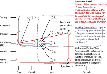
The Working Group discussed the conundrum of needing to demonstrate associations between use and resistance in order to gain support to conduct surveillance. This conflicts with having little real data to parameterize models to determine whether an association exists, resulting in circular discussions. Ultimately, the group determined that this was an epidemiologic question of association between an outcome (typically a disease outcome; in this case, AMR) and one or more explanatory factors (or risk factors; in this case specifically focused on AMU in livestock). Further refining the concept of association to focus on explaining observed variation, the Working Group decided that the fundamental scientific question was “What proportion of the observed variation in antimicrobial resistance within bacteria in the food supply can be explained by the observed variation in antimicrobial use in food-producing animals?” (Fig. 1).
Temporal scale and hierarchical levels at which the scientific questions were posed. The figure indicates (a) the hierarchical level(s) of Use (U) or Resistance (R) of questions posed as indicated by circles and (b) the possible levels to which resistance is implied by the question. For example, the question posed in the US National Action Plan for Combating Antibiotic-Resistant Bacteria points to the development of resistance, which can occur or be influenced at several levels. The initial Working Group posed question addresses resistance at the population level, which could be at the food animal (FA) or societal level, if measuring resistance in the human population. The currently posed question specifically examines resistance at the bacterial level in the food supply and whether any change in that resistance can be attributed to changes in antimicrobial use in the FA populations. Solid boxes capture individual questions (where the only temporal aspect is the implied use before resistance); dashed boxes indicate the temporal scope of answering the questions and the hierarchical level indicates the data required to answer the questions.

There are several important points to note regarding this question. First, the Working Group discussed making the distinction between association and causality, the former being necessary but not sufficient for the latter.
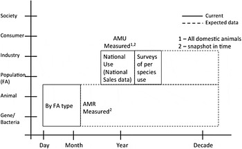
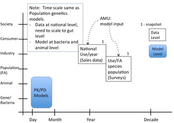
Second, the currently available data are measured at many levels (Fig. 2). As well as potentially missing subtle individual-level effects due to aggregation (and sampling delay), the population-level focus of this question raises concerns of the ‘ecological fallacy.’ This relates to the potential for an effect to be observed at the population level even though there is no effect at the individual level. Thus, while these methods are intended to detect national-level associations, they do not allow us to fully understand underlying mechanisms.
Temporal scale and hierarchical levels at which data are currently measured. Current measures (solid boxes) of the exposure – antimicrobial use (AMU) – are derived from yearly national sales data for food animal (FA) antimicrobials. Current indicators of antimicrobial resistance (AMR) are measured for the type of FA. Both measures provide a snapshot in time (point estimates) of the item measured. Initial models must make assumptions about the extent of time these point estimates cover until more temporal coverage data are obtained. Dashed boxes indicate the data expected to be available for model use in the future.

Third, the outcome (‘AMR within bacteria in the food supply’) is actually a collection of several factors tested on each experimental unit (i.e., it is a multivariate outcome). For example, individual bacterial colonies are typically tested for susceptibility to a long (but nowhere near exhaustive) list of antimicrobials, using one or more different techniques (e.g., broth microdilution assay and/or whole genome sequencing, etc.). This has bearing on the techniques appropriate for analyzing these data.
Fourth, the explanatory factor (‘AMU in food-producing animals’) is neither the biological interaction of interest (exposure of bacteria to antimicrobials), nor does it have a consensus measure. Knowledge of the biology of AMR and the animal-derived food supply system is thus critical to identify the most appropriate measures to characterize this explanatory factor.
Several approaches to model select subsystems of the overall AMU/AMR system were discussed. All have advantages and disadvantages. While simplicity is desired and often requested, the Working Group concluded that no one model could adequately address all aspects of the AMU/AMR system at the same time. Rather, a suite of subsystem models is necessary to provide estimates of uncertainty around the conclusions about associations between AMU and AMR and the effectiveness of policies which may affect either or both. These models can be used independently to answer questions geared toward a specific section of the system or in a combined manner to address questions geared toward the more complete system.
Scope and System Boundaries
Setting the boundaries for the AMR system in this project was both critical and challenging. While policy makers often desire simplicity in systems, to analyze the AMR system appropriately requires addressing the complexity of reality, yet communicating the findings from the model in a simple manner.
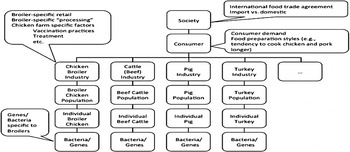
The following list, though not exhaustive, highlights why the AMR system is complex. The relationship between AMU in FAs and AMR in food products is not well understood. Many antimicrobials are used (for production purposes or therapeutically) in FA. Antimicrobials are currently used both singly and in combinations, including in combinations with heavy metals. There are numerous FA types, such as cattle (dairy, beef, veal), chickens (broilers, table egg layers), turkeys, pigs, shellfish, finfish, sheep, goats, etc. Numerous food products are derived from each FA; for example, from cattle, steaks, organ meat, veal, ground beef, and tartar can be produced. Food processing factors, either at or before retail, must be included in a comprehensive approach to investigating the association between AMU and AMR. Antimicrobial-resistant bacteria occur naturally and more species and strains of these bacteria will continue to emerge. Hence, the framework for the study of AMU/AMR should be sufficiently generalizable for future inclusion of new bacteria, resistant strains, and drugs. In addition, numerous genes confer AMR (e.g., dozens of tet genes confer resistance to tetracyclines). Some genetic elements are chromosomal in nature and some are carried on transferable elements (plasmids, transposons, integrons, etc.). Figure 3 illustrates just part of the hierarchies (and aspects within them) involved in answering the AMU/AMR association question, looking only at FA.
Hierarchical nature of the food animal (FA) industry and factors impacting antimicrobial resistance (AMR) with FA-specific factors. Pressures on AMR have many factors dependent on the specific FA and at different scales within the FA industry, consumer and society. For instance, using the lens of broiler chickens, there are resistance genes and bacteria specific to broilers, and commensals and pathogens of public health concern. Broiler-specific factors include vaccination practices, antimicrobial treatment, etc. At the consumer level, demand for specific product types and food preparation styles play a role. At the societal level, factors like international trade agreements and whether a food item is imported or domestic play a role.

In terms of scale, first, population-level effects, particularly at the national scale, were the primary interest of this project. This is not to say that finer scales (e.g., animal and pathogen) of the system are not important, in fact they are likely critical to understanding the issue. However, the Working Group was tasked with focusing on AMU and AMR at the national level. The relevance of international aspects (including movement of people, animals, food products, and drugs) is well-documented, but outside the scope of this particular project. Hence, the geospatial upper bound of our system was the continental USA. The lower bound was the genetic/molecular level.
Second, the National Antimicrobial Resistance Monitoring System (NARMS) provided additional system boundaries, which were both appropriate for this project and practical in terms of data availability. These bounds included: bacteria (i.e., Salmonella, Campylobacter, Escherichia coli, and Enterococcus), animal species (i.e., those that the FDA considers the ‘major food species’: cattle, swine, chickens and turkeys), and sampling sites (e.g., animals at slaughter and retail meat). Although NARMS also samples clinical isolates from humans with enteric infections (Centers for Disease Control and Prevention, 2016), that part of the risk pathway was excluded from the scope of this project due to its distance from the primary biological point of interest (i.e., the lower gastrointestinal tract of FAs) and the expectation that observed effects at this site would be greatly ‘diluted’ by other factors pertinent to human populations. Use of antimicrobials in human medicine is similarly beyond the scope of this project.
Regarding the scope of drugs, the specific drugs NARMS evaluates within the abovementioned target bacteria are based mainly on human clinical relevance, and do not necessarily cover all drugs (or even drug classes) directly impacted by Guidance for Industry (GFI) 213, an FDA document spelling out the processes needed to limit medically important antimicrobials to uses in FA considered necessary to ensure health and that include veterinary oversight or consultation. Furthermore, since we might anticipate (and be greatly interested in) changes in resistance to drugs that are not directly impacted by this (or any other) specific intervention, we are expanding our drugs of interest beyond the NARMS panels to all antimicrobial new animal drugsFootnote 2 approved by the FDA for use in FA. This excludes compounds with antimicrobial activity, which are not considered ‘new animal drugs’ (e.g., disinfectants) or otherwise not currently regulated by the FDA.
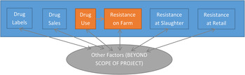
Hence, for this project, the following system restrictions were applied: inclusion only of foodborne bacteria, the major FA species (cattle, pigs, chickens, and turkeys), and the selective pressures due to drug use in FA (Fig. 4). The scientific question posed includes food processing factors as part of the pathway between use and resistance, but current surveillance provides insufficient data to determine the scale of influence of the processing factors. Environmental and climatological factors were not included at this time.
Summary of the scope of this project using the foodborne antimicrobial resistance risk pathway; red = primary focus, blue = in scope, gray = beyond the scope (e.g., disinfectant use in slaughter plants may be linked with some resistances; non-antimicrobial changes in management practices; consumer demand).

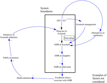
Figure 5 shows boundaries for the food supply system. As the boundary on the system under study becomes tighter, one might think that model results will become more precise. That may sometimes be true, but the Working Group agreed that accuracy is more important than precision in the AMR system.
An example of boundary setting for food supply system (GFI = Guidance for Industry; AMR = antimicrobial resistance). The rectangle denotes the system boundaries. The factors outside the box (public awareness, etc.) were beyond the scope of the AMR system model in this project.

Analytic methods needed to model the system or subsystem(s) of interest
The following subsystems and methods were identified as critical components of our analytic framework.
Antimicrobial use in food animals
Described factors impacting AMU in FA; reviewed indices for AMU; and presented methods for how exposure of enteric bacteria within the animals to the antimicrobials or their active metabolites can be estimated (extending the animal-level estimates to represent the actual antimicrobial exposure of foodborne pathogens).
Phenotypic resistance in bacteria in the animal-derived food supply
Identified methods to model changes in antimicrobial susceptibility of bacteria isolated from various stages in the animal-derived food production system (e.g., farm, slaughter, and retail).
Genotypic resistance in bacteria in the animal-derived food supply
Identified methods to model changes in genotypic patterns associated with antimicrobial susceptibility of bacteria isolated from various stages in the animal-derived food production system (e.g., farm, slaughter, and retail)
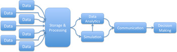
Then, the subsystems were brought together within an overall Systems Approach (a separate method unto itself), which identified methods and considerations for system assumptions, system to be modeled, data requirements, model [result] integration, system boundaries, uncertainties associated with models/model levels/data availability, information needed, and the overall model framework.
The following describes each of the subsystems and overall system. Select aspects of the models were evaluated with existing data (the performance of the models) and for each subsystem additional needed data were identified, which were the most important for improving the performance of the particular model.
Subsystem – antimicrobial use in food animals
Factors affecting the use of antimicrobials in food animals
Many factors affect the use of antimicrobials in FA. These include: (1) the FA population structure such as the numbers of farms and animals of individual species, production classes (e.g., breeder and finisher), and types of production (e.g., organic); (2) the incidence of animal health conditions necessitating AMU for disease prevention, control, therapy, or improving production efficacy; (3) the observation and detection of the animal health conditions, risk perception, responsiveness to intervene by animal caregiver or veterinarian; (4) the antimicrobial arsenal per label and extra-label use allowance given the animal species, production class, type of production, and the health condition; (5) the decision-making/choice of the antimicrobials by the caregiver or veterinarian, including personal perceptions, experiences, and societal pressures; (6) the economics and implementability of the AMU choice; and (7) the availability, economics, and implementability of alternative drugs or management approaches to avert or manage the health condition.
Indices of antimicrobial use in food animals on farms
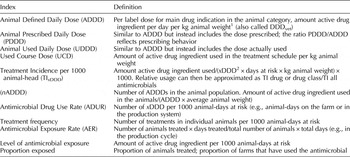
Various indices have been proposed to describe animal AMU (Bager et al., Reference Bager, Madsen, Christensen and Aarestrup1997, Reference Berge, Moore and Sischo2006; Dunlop et al., Reference Dunlop, McEwen, Meek, Black, Clarke and Friendship1998; Kruse et al., Reference Kruse, Johansen, Rorvik and Schaller1999; Jensen et al., Reference Jensen, Jacobsen and Bager2004; Chauvin et al., Reference Chauvin, Le Bouquin-Leneveu, Hardy, Haguet, Orand and Sanders2005; Grave et al., Reference Grave, Jensen, McEwen, Kruse and Aarestrup2006; Timmerman et al., Reference Timmerman, Dewulf, Catry, Feyen, Opsomer, de Kruif and Maes2006; Carson et al., Reference Carson, Reid-Smith, Irwin, Martin and McEwen2008; Harada et al., Reference Harada, Asai, Ozawa, Kojima and Takahashi2008; Varga et al., Reference Varga, Rajic, McFall, Reid-Smith, Deckert, Checkley and McEwen2009a, Reference Varga, Rajic, McFall, Reid-Smith and McEwenb; Deckert et al., Reference Deckert, Gow, Rosengren, Leger, Avery, Daignault, Dutil, Reid-Smith and Irwin2010; Moon et al., Reference Moon, Berke, Avery, McEwen, Reid-Smith, Scott and Menzies2011; Vieira et al., Reference Vieira, Pires, Houe and Emborg2011; Apley et al., Reference Apley, Bush, Morrison, Singer and Snelson2012; Callens et al., Reference Callens, Persoons, Maes, Laanen, Postma, Boyen, Haesebrouck, Butaye, Catry and Dewulf2012; CIPARS, 2012; DANMAP, 2014; Garcia-Migura et al., Reference Garcia-Migura, Hendriksen, Fraile and Aarestrup2014; Merle et al., Reference Merle, Robanus, Hegger-Gravenhorst, Mollenhauer, Hajek, Käsbohrer, Honscha and Kreienbrock2014; MARAN, 2014; SVARM, 2014; Benedict et al., Reference Benedict, Gow, McAllister, Booker, Hannon, Checkley, Noyes and Morley2015; Postma et al., Reference Postma, Sjölund, Collineau, Lösken, Stärk and Dewulf2015; Noyes et al., Reference Noyes, Benedict, Gow, Waldner, Reid-Smith, Booker, McAllister and Morley2016; Stevens et al., Reference Stevens, Piepers, Supré, Dewulf and De Vliegher2016). Commonly used indices are summarized in Table 1. Other indices have been applied for specific uses, e.g., number of intra-mammary doses or the treated disease case rate in the population.
Examples of indices that have been used to describe animal antimicrobial use

1 The indices listed have been standardized as the active drug ingredient amount per kg animal meat, kg animal live weight, or Population Correction Unit (PCU). The PCU is defined as kg live or slaughtered animal weight for the animal category, estimated as the number of live or slaughtered animals × standard or average animal weight at most likely time of the antimicrobial administration (European Medicines Agency ESVAC, 2015).
2 xDDD – either ADDD or PDDD or UDDD.
Indices in Table 1 can describe AMU in a FA category for a farm, region, or country when quantities and frequencies of the antimicrobials used are known. In the absence of such data, some countries use an approach based on the drug's main indication for the FA category: per label drug dosage and schedule are used to derive the Animal Defined Daily Dose (ADDD) and Used Course Dose (UCD); this is combined with the total drug amounts used or sold and population characteristics (number and weight of animals) to approximate the drug use intensity – number of ADDD (nADDD) or Antimicrobial Drug Use Rate (ADUR). Few national surveillance systems collect data on AMU or antimicrobial sales for individual FA species (CIPARS, 2012; ANSES, 2014; DANMAP, 2014; MARAN, 2014; SVARM, 2014); these data have been collected in different manners, for example on farms, from veterinarians, or from pharmacies. Other countries collect only data on total antimicrobial sales for veterinary use (HPRA, 2014; ESVAC, 2016; EVIRA, 2016). Indices to approximate AMU based on the total sales have been proposed, for example Animal Level of Exposure to Antimicrobials (ALEA) for a given FA species (ANSES, 2014). Methods are being developed to stratify the total veterinary antimicrobial sales by animal species, utilizing supportive farm-level AMU data and re-partitioning the sales based on the animal body mass and veterinary prescription patterns (Carmo et al., Reference Carmo, Schüpbach-Regula, Müntener, Chevance, Moulin and Magouras2015).
The USA currently collects data on total veterinary antimicrobial salesFootnote 3 (FDA, 2015). Data on estimated antimicrobial sales for individual FA species will be collected by the FDA starting in 2016 and reported in 2017. Another data source on AMU in FA in the USA are studies conducted by the National Animal Health Monitoring System (NAHMS) of the Animal and Plant Health Inspection Service (APHIS) of the USDA. The main purpose of national-level NAHMS studies is to monitor FA health and production practices, including frequency and management of specific health conditions. For a given FA species, the NAHMS study is conducted on a rotating 5–10-year cycle. Objectives of each study are determined by a needs assessment with stakeholders. Several of the NAHMS studies have included surveys of antimicrobial drug choices for managing animal health and the purposes of AMU.
Relationship between antimicrobial use in food animals and antimicrobial exposure of enteric bacteria within the animals
In FA administered antimicrobials, enteric bacteria are exposed to concentrations of the drugs or their antimicrobially active metabolites that are excreted or passed with the digesta to the intestine. Antimicrobials vary in their metabolism and excretion, and in the processes these drugs and active metabolites undergo in the intestine (e.g., degradation). Thus, the fraction of the administered drug that is in the intestine in active form varies by drug and its formulation, is influenced by a number of further factors (Volkova et al., Reference Volkova, KuKanich and Riviere2016), and relates non-linearly to the quantity administered at the animal level. The concentrations of drugs/active metabolites in the intestine can be determined using animal- or population-level pharmacokinetic (PK)-for-intestine models (Volkova et al., Reference Volkova, Lanzas, Lu and Gröhn2012; Cazer et al., Reference Cazer, Volkova and Gröhn2014; Volkova et al., Reference Volkova, KuKanich and Riviere2016). Experimental studies have started providing in vivo estimates of the intestinal concentrations of antimicrobials (Foster et al., Reference Foster, Jacob, Warren and Papich2016). Combinations of such modeling and experimental efforts can fill the knowledge gap on the antimicrobial exposure of enteric bacteria within animals due to AMU. The effects on enteric bacteria and their AMR from the exposure can be studied using pharmacodynamic (PD) models. Combined modeling of the drug's PK-for-intestine and PD for enteric bacteria can enable evaluating the impact of interventions regarding AMU in FA on AMR in foodborne pathogens.
Figure 6 depicts the levels at which data are required for operation of these models, where the data exist, where the models operate, and at what level the modeling results can answer the AMR question posed in the introduction.
Pharmacokinetic/pharmacodynamic (PK/PD) models. Currently, antimicrobial use (AMU) is surveyed by the US National Animal Health Monitoring System at farm and food animal (FA) levels as point estimates. PK-for-intestine models can be used at animal and population levels to extrapolate to the animals’ intestines, to estimate antimicrobial exposure of enteric bacteria within the animals due to AMU in the animals. PD models can then be used to estimate effects from antimicrobial exposure on enteric bacteria and their antimicrobial resistance (AMR). Outputs that can be derived from PK/PD modeling are changes in AMR at the bacteria, individual animal, and animal population levels.

Example – evaluation of this approach – exploratory work
The following example illustrates estimation of population-level antimicrobial exposure of enteric bacteria in a specific FA production stage, by combining the estimates of a select drug's use in the animals with the PK-for-intestine model. The example also shows the differences in the results provided by various indices for describing AMU at the animal level (Table 1). The example is based on use of a third-generation cephalosporin (ceftiofur) to prevent or control shipping fever in beef feedlot cattle. Ceftiofur use at the animal level was approximated based on the data from a survey of beef feedlots with headage >1000 conducted by the USDA APHIS NAHMS in 2011 in 12 US continental states (USDA APHIS NAHMS, 2011a, b, c). Such feedlots housed 82% of the US beef cattle inventory in 2011 according to the National Agricultural Statistics Service. Of those cattle, 95% were in the 12 states surveyed. Hence, the population surveyed included ~78% of the US beef cattle. In this population, ~60% of cattle were on feedlots with <8000 and ~40% on feedlots with ≥8000 headage. Approximately half of the cattle put on feed in 2011 had an initial body weight (BW) below and the other half above 700 lb (318 kg); we assumed this was similar for feedlots with headage <8000 and ≥8000. For these four animal categories the survey reported the frequency of health conditions necessitating AMU, and frequency of specific antimicrobial choices by purpose. For illustrative purposes, we considered a random sample of 1 million cattle from this population maintained on feed for 6 months. From the survey data, the estimated proportions of cattle treated with an injectable antimicrobial for prevention or control of shipping fever were: 27% of animals placed on feed with a BW < 700 lb on feedlots with headage <8000; 4% of animals at BW ≥700 lb on feedlots with headage <8000; 41% of animals at BW<700 lb on feedlots with headage ≥8000; and 5% of animals at BW ≥ 700 lb on feedlots with headage ≥8000. Ceftiofur was the drug of choice for the estimated 26% of those treated on feedlots with <8000 and 13% on feedlots with ≥8000 headage; we assumed this was similar for cattle with BW below and above 700 lb at placement. We assumed an animal received one ceftiofur treatment (a non-sustained-release drug formulation) by injection for this purpose during the 6 months on feed, following the label daily dosage of 2.2 mg kg−1 BW for 5 days.
We considered that an average or standard animal in the feedlot system weighed 800 lb (363 kg). For the categories placed on feed with BW below and above 700 lb, we considered a 650 lb (295 kg) BW animal and an 850 lb (386 kg) BW animal, respectively, receiving the 5-day ceftiofur treatment. Further, a simplified assumption was made to enable the illustrative estimations, that at the time of ceftiofur treatment all cattle placed on feed at BW < 700 lb weighed 650 lb, all cattle placed on feed at BW > 700 lb weighed 850 lb, and, to consider the overall population – all cattle were of average BW of 800 lb at the time of treatment. Table 2 summarizes the estimated animal-level indices of ceftiofur use for these two sub-categories of weight and for the overall population. If appropriate, the indices were standardized by kg of animal live BW at the time of drug administration. The estimates (Table 2) highlighted that the AMU indices standardized per kg of animal BW do not reflect differences in the antimicrobial exposure at the animal level arising from the differences in BW at the time of drug administration.
Use of ceftiofur for prevention or control of shipping fever in US beef feedlot cattle – at the animal-level and various population-levels

BW, body weight; ADDD, Animal Defined Daily Dose; UCD, Used Course Dose; ADUR, Antimicrobial Drug Use Rate; AER, Antimicrobial Exposure Rate; MIL, Million.
1 Drug – active ingredient amount.
Ceftiofur is rapidly metabolized in the animal body; a large fraction of the metabolites retains antimicrobial activity (Ritter et al., Reference Ritter, Kirby and Cerniglia1996; Salmon et al., Reference Salmon, Watts and Yancey1996; Hornish and Kotarski, Reference Hornish and Kotarski2002). Utilizing a published model of ceftiofur PK-for-intestine that is based on experimental data (Beconi-Barker et al., Reference Beconi-Barker, Roof, Vidmar, Hornish, Smith, Gatchell and Gilbertson1996; Volkova et al., Reference Volkova, Lanzas, Lu and Gröhn2012), we assumed 25–35% of the active ingredient administered daily to cattle can reach their lower intestines in the form of the antimicrobially-active metabolites excreted in bile. The metabolites likely undergo biotic degradation by enzymes produced by enteric bacteria to antimicrobially-inactive compounds (Gilbertson et al., Reference Gilbertson, Hornish, Jaglan, Koshy, Nappier, Stahl, Cazers, Nappier and Kubicek1990; Hornish and Kotarski, Reference Hornish and Kotarski2002). We assumed the degradation occurred for 6 h before the metabolites reach the lower intestine, and used a published estimate of the degradation rate (Volkova et al., Reference Volkova, Lanzas, Lu and Gröhn2012). The projected quantities of the active metabolites reaching the lower intestine daily were 49–68 mg in a 650 lb and 64–89 mg in an 850 lb animal (Table 3). Further, we used a published allometric model to approximate the volume of cattle large intestine based on BW (Cazer et al., Reference Cazer, Volkova and Gröhn2014). Given the metabolite quantities, their degradation, and intestinal volume, projected maximum concentrations of the active metabolites in the lower intestine were 1.7–2.4 µg ml−1 in either a 650 or 850 lb animal (these concentrations occurred after each of the five daily injections) (Table 3). The estimated concentrations compared well with experimental data (Foster et al., Reference Foster, Jacob, Warren and Papich2016). Thus, even though the metabolite quantities reaching the intestine may be higher in an animal with larger BW, the antimicrobial concentration to which enteric bacteria are exposed may be similar to that in a smaller animal treated under the same schedule (because of associated differences in the intestinal volume).
Use of ceftiofur for prevention and control of shipping fever in US beef feedlot cattle

Estimates of the antimicrobial exposure of enteric bacteria of the lower intestine for individual cattle, and hypothetical (based on a hypothetical No Observable Effect Level (NOEL)) estimates of the population-level indices summarizing the exposure of enteric bacteria for the population, and sub-categories of the population in terms of the body weights when placed on feed.
BW, body weight; MIL, million.
1 Metabolites – amount of antimicrobially active ceftiofur metabolites.
2 Selective pressure – occasion when the concentration of the antimicrobially active ceftiofur metabolites in lower intestine(s) exceeds the NOEL.
Next, we proposed three population-level indices of antimicrobial exposure of enteric bacteria within animals due to AMU in the FA category (population of interest); the illustrative estimates of the indices for the example of ceftiofur use for prevention and control of shipping fever in beef cattle are given in Table 3. The first index is the projected quantity of the drug/its active metabolites reaching the animal lower intestines, standardized per 1000 animal-days. In the example, it is estimated by summing the quantities of active ceftiofur metabolites reaching the lower intestines during the 5-day schedule in all cattle administered the schedule, standardized per 1000 total animal-days during the 6 month production cycle. Yet, as shown above, antimicrobial concentrations in the lower intestine may be similar in animals in which the antimicrobial quantities reaching the intestine are different (because of the allometric relationships between animal body size and intestinal volume).
A concept of an antimicrobial's No Observable Effect Level (NOEL) has been proposed (Perrin-Guyomard et al., Reference Perrin-Guyomard, Cottin, Corpet, Boisseau and Poul2001; FDA-CVM, 2004, 2012; Carman et al., Reference Carman, Simon, Petzold, Wimmer, Batra, Fernandez, Miller and Bartholomew2005). We considered that the NOEL may be defined as the maximum antimicrobial concentration in the intestines in the FA category at which there are still no observable (measurable by currently available methods) effects on the intestinal microbiome's structure, or, alternatively, on the microbiome's resistome (the entirety of AMR genes in the bacteria). (The NOEL may also be defined for a specific enteric bacterial species, as the maximum antimicrobial concentration in the intestines in the FA category, at which there are still no observable effects on AMR in that bacterial species). We derived the other two candidate population-level indices of selective exposure on enteric bacteria within animals in the FA category due to use of the antimicrobial in the animals as: (1) duration of selective pressure, the total hours the antimicrobial's concentrations in the lower intestines of treated animals in the FA category exceeded the antimicrobial's NOEL, standardized by the total animal-hours in the FA category in the period of interest; and (2) the frequency of selective pressure, the total number of days the antimicrobial's concentrations in the lower intestines in treated animals in the FA category exceeded the antimicrobial's NOEL, standardized by total animal-days in the FA category in the period of interest.
For the example, we defined the NOELresistome as the concentration of antimicrobially active ceftiofur metabolites in the lower intestines of beef feedlot cattle at which there are still no detectable changes in the intestinal microbiome's resistome. We hypothetically assumed the NOELresistome was 0.05 µg ml−1. Given the projected active metabolite concentration dynamics in the lower intestines (as detailed above, utilizing a model of ceftiofur PK-for-intestine (Volkova et al., Reference Volkova, Lanzas, Lu and Gröhn2012) and experimental data (Foster et al., Reference Foster, Jacob, Warren and Papich2016)), the concentrations exceeded the hypothetical NOELresistome for 18 h each day of the 5-day schedule in either a 650 or 800 or 850 lb animal. With these assumptions, we derived:
-
(1) Duration of selective pressure: Total hours the concentrations of antimicrobially active ceftiofur metabolites in the lower intestines of cattle that received the 5-day ceftiofur schedule for shipping fever control exceeded the NOELresistome per 100,000 total animal-hours in the 6 months on feed considered. The estimates are given in Table 3.
-
(2) Frequency of selective pressure: Total number of days in cattle that received the 5-day ceftiofur schedule for shipping fever control when the concentrations of antimicrobially active ceftiofur metabolites in the lower intestines exceeded the NOELresistome per 1000 total animal-days in the 6 months on feed considered. The estimates are given in Table 3.
This example outlines the methods that could be used to estimate the selective pressure on enteric bacteria of FA receiving antimicrobials (for any purpose), directly assessing the pressure relevant for AMR in foodborne pathogens. The selective pressure as a proportion of the AMU at the animal (or animal aggregate on farms) level will differ among antimicrobial drug classes and individual drugs and their formulations. Generalizable frameworks for theoretically comparing antimicrobials in the pressure extorted on enteric bacteria (Toutain et al., Reference Toutain, Ferran, Bousquet-Mélou, Pelligand and Lees2016) and for developing the PK-for-intestine models to estimate the selective pressure (Volkova et al., Reference Volkova, KuKanich and Riviere2016) have been laid down. Once the models are developed for representative drugs of each class, administration route, and FA species, accumulation and standardization of the data and modeling techniques streamlining further applications will be possible. The outputs as the selective pressure indices (as in the example above) for animal groups and populations can directly enter epidemiological and systems analyses, and be tested for associations with AMR outcomes in specific foodborne pathogens. The latter outcomes can be captured via the phenotypic and genotypic methods outlined in Sections ‘Subsystem – Evaluation of Phenotypic Antimicrobial Resistance in the Food Supply’ and ‘Subsystem – Evolutionary Genetic Perspectives on Antimicrobial Dynamics’, respectively. Alternatively, the selective pressure indices for enteric bacteria in FA can be defined via the NOEL or similar metrics. Estimating the NOEL for the resistome of the enteric microbiome (or the entire subset of potential foodborne pathogens in it) for major FA species, age groups, and antimicrobials could be cost-effective in terms of research investment compared to tracing the impact on each pathogen (densities and antimicrobial susceptibilities of the pathogens vary greatly within and between FA species and sub-populations). The example shows that this approach can provide significant insights into associating and choosing resistance mitigation approaches that target AMU in FA to mitigate AMR. In the example, the selection pressure on enteric bacteria in hours and days was greater for lighter animals than for heavier animals treated by the same antimicrobial and protocol in one production system. Hence, these types of models can enable creating population-specific therapeutic guidelines, which directly consider the selective pressure of the antimicrobial on enteric bacteria, offering more precise and better targeted antimicrobial stewardship recommendations.
Subsystem – evaluation of phenotypic antimicrobial resistance in the food supply
Current data availability
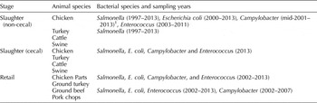
The NARMS tests antimicrobial susceptibility of human clinical isolates of enteric pathogens and bacteria in retail meats and FA. The NARMS public-release isolate-level data contain susceptibility test results for each isolate (105,922 isolates in total) from samples collected at slaughter and in participating states, at the retail level (Table 4). NARMS reports minimum inhibitory concentrations (MICs) for a panel of antimicrobials tested for each isolate. The MIC is usually measured by a broth microdilution method; an isolate's growth is evaluated when exposed to successive 2-fold dilutions of antimicrobials. The test outcome, the MIC, is the lowest concentration with no visible growth after a specific time period, so the MIC for each bacteria–antimicrobial combination is a discrete variable. To aid interpretation of the susceptibility tests, MICs are often categorized into three classes (susceptible, intermediate, and resistant) using breakpoints.
Animal and bacterial species data available in the National Antimicrobial Resistance Monitoring System (NARMS) dataset

1 Isolation of Campylobacter from chicken at slaughter began in 1998, but nalidixic acid susceptibility and cephalothin resistance were used by the USDA as identification criteria for Campylobacter jejuni/coli until mid-2001, which likely resulted in underreporting of quinolone-resistant Campylobacter during this time period.
Surveillance data collected before implementation of the FDA's interventions provide a baseline to compare changes in resistance outcomes. Changes in AMR levels after the policy implementation might be linked to the policy.
Analytic methods – strengths and limitations
Trends in AMR phenotypic changes observed through NARMS are often analyzed and summarized using univariate approaches such as the percentage of non-susceptible isolates to drugs of interest in bacteria species for which resistance is of great concern. Clinically, this is an important and useful parameter to help guide therapy, but it is less informative for monitoring effects of mitigation strategies on resistance for several reasons, including: (1) changes in MIC distribution that do not occur near the breakpoints may go undetected; (2) the background prevalence of resistance is high for some combinations of antimicrobials and bacteria species, making detection of changes due to mitigation strategies difficult, as stochastic variation may be large; and (3) for Salmonella specifically these percentages are highly influenced by serotype composition of the sample.
Metrics identifying shifts in resistance should be refined; common ones such as percentage resistant based on breakpoints are not the most sensitive ones to evaluate resistance trends. The MIC values themselves may be a better choice than categorizing MIC as susceptible or non-susceptible. Also, NARMS data are multivariate. Each isolate has an MIC value for each antimicrobial in the panel. The number of antimicrobials included in a given panel varies by bacteria and year and ranges from 9 to 16 drugs. Covariance between MIC values is likely to be positive for some drug–bacteria combinations. Some drugs share biochemical mechanisms that confer resistance. Other drugs can be positively correlated if genetic linkage exists between their resistance genes. Frequency of multidrug resistance thus exceeds what would be expected by chance. Methods that expand beyond univariate approaches are needed to understand relationships among antimicrobials.
Resistance patterns have been analyzed using multivariate methods, e.g., principal component analysis or factor analysis (Wagner et al., Reference Wagner, Salman, Dargatz, Morley, Wittum and Keefe2003; Jaspers et al., Reference Jaspers, Ganyani, Ensoy, Faes and Aerts2016). These have been used to reduce the measured variables into fewer components that capture data variability. The main limitation of multivariate approaches that perform dimension reduction is the difficulty in interpreting the meaning of the created variables. Principal components are easier to interpret when clear separation of antimicrobials exists among principal components, e.g., if each principal component represents a drug class (Poupard et al., Reference Poupard, Brown, Gagnon, Stanhope and Stewart2002).
Graphical modeling can represent the multivariate relationships that exist within MIC data without performing dimension reduction. Markov networks, a form of undirected graphical models, can be used to represent variables in a set of data, where the variables are the vertices and the correlations between variables are represented by edges connecting the vertices (Taskar and Getoor, Reference Taskar and Getoor2007). In applying graphical models to NARMS data, a vertex represents each drug resistance and edges joining drugs indicate drugs that are not conditionally independent. The most common types of graphical models are Bayesian networks (BNs) and Markov networks.
Example – evaluation of phenotypic modeling approaches to evaluate interventions
Our exploratory work had two phases. The first focused on variation of resistance to individual antimicrobials (Zawack et al., Reference Zawack, Li, Booth, Love, Lanzas and Gröhn2016) and the second on patterns of co-occurrence of resistance for multiple drugs (Love et al., Reference Love, Zawack, Booth, Gröhn and Lanzas2016).
The aim of the first phase was to study baseline AMR and how the information gained can be used to assess changes in policy. To do this, we studied historical NARMS data (2004–2012), looking at various microbe, host, and antimicrobial combinations. Having gained an understanding of the variation in these data, we wanted to know how much data should be collected to find a statistically significant difference in resistance, before and after a policy change. Our objectives were to: (1) evaluate the baseline trend and variations in the NARMS data; (2) examine the structure of the variation in resistance within/between years, and across geographic regions; and (3) using this baseline, estimate how much data must be collected to determine if the change in FDA policy had an effect.
The aim of the second phase was to develop methods to describe patterns in multidrug (>1 antimicrobial in the resistance pattern) resistance (MDR) and how these patterns change over time. Our objectives were to: (1) estimate the Markov networks describing AMR relationships using the graphical least absolute shrinkage and selection operator (lasso); (2) apply log-linear models of contingency tables to infer more complex multi-drug relationships; and (3) understand how these patterns have changed across time.
Phase 1
To gain a basic understanding of AMR changes over time and across slaughter and retail in the food supply chain, we explored resistance data for each microbe/host/antimicrobial combination (Zawack et al., Reference Zawack, Li, Booth, Love, Lanzas and Gröhn2016). We focused on chicken as the host species and resistance of Campylobacter jejuni to tetracycline, C. coli to erythromycin, Salmonella Typhimurium to ampicillin, and E. coli to streptomycin. Chicken had the most consistent data across all time points and stages. Bacteria were chosen for their significance as pathogens, number of observations, and MIC distribution patterns. The time frame of 2004–2012 was chosen because both slaughter and retail data for chicken were available then.
To assess AMR trends, we built simple models of resistance with AMR as a binary variable in logistic regression and as a censored continuous variable in linear regression, using log2 (MIC). We used logistic regression to model the log odds of resistance versus non-resistance as a function of slaughter/retail and year. We also treated MIC as continuous, and mean log2 MIC was modeled as a linear function of stage and year. To study the sources of variation in resistance, log2 MIC was modeled as a function of a fixed intercept for state and a random intercept for year, in a linear fixed effects model.
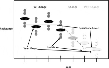
To evaluate the effectiveness of the FDA policy change in line with our analyses, we created a model with a constant base level of resistance around which yearly levels varied, a period of change, and then anticipated that a new resistance level would be established (Fig. 7). A hypothesis test of mean resistance level before and after policy change can assess change in resistance. Different variation within and between years was assumed; hence, the test was carried out on mean yearly resistance. This test can be done with either percent resistance or MIC values. Power analysis was performed to benchmark the test's efficacy. Calculating power requires knowledge of standard deviation (SD), sample size, and magnitude of the effect to be detected. For the t-test of mean log2 MIC, SDs were chosen by calculating the empirical distribution for the SD of the mean log2 MIC per year. Number of isolates per year was assumed to be 200, a number generally exceeded in historical data. The current 9 years of data were used as pre-policy change sample size. Post-policy change, sample sizes were assumed to be between 1 and 10 years. The desired detectable effect was taken to be between 0 and 1 log2 MIC. Power curves were drawn.
The model of antimicrobial resistance used in evaluating policy changes. It is assumed there is a constant base level of resistance around which the yearly levels vary, a period of change, and then a new resistance level is established.

Resistant/susceptible counts are binomial quantities; their SDs are functions of proportions. Data are from a mix of conditions such as geographical location, season, and production quality, so the proportions are overdispersed with respect to binomial variation; the SD will also be a function of this overdispersion parameter. Plotting the empirical distribution of each quantity yielded reasonable proportions and overdispersion parameters. Isolates per year was set to 200, pre-policy change sample size was 9 years, post-change sample size was between 1 and 10 years, and effect sizes were chosen to be detectable with such sample sizes.
Phase 2
To study collateral resistance patterns we used the resistance measurements for all drugs against E. coli from chickens at both slaughter and retail. Collateral resistance is the positive or negative impact of one drug resistance trait on other resistances. When a bacteria population is exposed to an antimicrobial, resistant bacteria are selected for and prevalence of resistance to the antimicrobial in the population increases. Other resistances correlated with the selected resistance will also change frequency in the population. We developed Markov networks to describe these collateral resistances and evaluated changes in resistance patterns (Love et al., Reference Love, Zawack, Booth, Gröhn and Lanzas2016). Presence or absence of specific edges at various times can provide information about resistance relationships between the specific drugs. Edges consistently present during the study period represent stable resistance relationships, and are expected to be found among drugs that share common mechanisms for resistance. For example, stable relationships are expected among drugs in the β-lactam class because β-lactamase enzymes are effective, albeit to varying degrees, in all drugs in the class. Edges that were absent during early time periods, yet which become consistently present in later time periods, may represent emergent patterns of drug resistance in the microbial population. The NARMS data were stratified by year; MIC values were log2 transformed. A Spearman rank correlation matrix of the transformed MIC values was calculated, and the associated penalized precision matrix was estimated using the graphical least absolute shrinkage and selection operator (GLASSO method) (Friedman et al., Reference Friedman, Hastie and Tibshirani2008). This step removed trivial partial correlations, making the resultant Markov networks sparser.
Modeling collateral resistance as graphical models provides a number of advantages. First, graphical models provide excellent visualization of the systems they represent. Another advantage is that a wide variety of parameters have been described to summarize the structure of networks. These parameters include but are not limited to: density, modularity, vertex degree, and vertex centrality. These parameters describe different structural characteristics and can be tracked over time to summarize structural trends. Algorithms also exist to find particularly dense subregions of networks. These correlate with sets of potentially important phenotypic resistance traits in Markov networks of resistance.
Building on the graphical models inferred using GLASSO, we examined the AMR data with a log-linear model, providing a different means of inferring pairwise dependencies and of inferring multi-way dependencies. Log2 MIC for each antimicrobial test was converted to a binary susceptible/resistant value and collected in a contingency table. A log-linear model was then built for the joint density of the cells in this table, using forward inclusion, manually enforcing the hierarchy principle.
Once we had a strong understanding of the MDR patterns in single years, we examined trends in the patterns over time. For the GLASSO models we inspected changes in the graphical model parameters. For the log-linear approach, year was included as a random effect.
Results
Slaughter and retail had similar trends. It was important to consider both AMR proportion and MIC; each captured different AMR changes over time. Most variation was within, not between, years; little additional variation was explained by accounting for geographic location (state) in retail data where this information was available. We estimated at current rates of data collection, a 1-fold change in MIC should be detectable in 5 years and a 6% decrease in percent resistance could be detected in 6 years following establishment of the new resistance rate. As most variation is within years, the number of isolates tested each year is important in determining this power. The current level of 200 samples per year provides a high degree of power; the standard power threshold of 0.8 could be achieved with 100 samples per year.
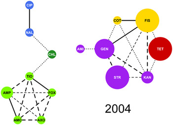
Figure 8 shows an example of a Markov network for MIC data for 2004. During the 9 years of the study, 33 unique edges of the 119 possible were identified, and 19 were present in 6 years or more. The remaining unique edges that were identified tended to be weak and only sporadically present. Graphical density describes the proportion of all edges that are present and represents overall graph interconnectivity (m = m obs/ k C2). The density of AMR Markov networks ranged from 16.2 to 24.8% and did not appear to change over time (Spearman's ρ = −0.14, P = 0.71). Modularity in these networks describes how frequently resistance to similar drugs was connected (Newman, Reference Newman2004; Gomez et al., Reference Gomez, Jensen and Arenas2009). Assortativity was always positive in these networks and did not change significantly over time (Spearman's ρ = −0.48, P = 0.18). Two subgraphs of high density appeared frequently. The first contained the β-lactam antimicrobials (penicillins and cephalosporins) and in all years was complete, that is, all possible edges were present (m = 5C2 = 10). The other dense subgraph contained sulfonamides, tetracycline and most of the aminoglycosides. This subgraph had a density of 50% or more in 6 of the 9 years in the study.
Markov network of drug resistance relationships in Escherichia coli isolated from chicken collected in 2004 and tested by the FDA and USDA. The following 15 drugs from the NARMS panel for E. coli were included in the graph: ampicillin (AMP), amoxicillin and clavulanic acid (AMC), ceftriaxone (AXO), cefoxitime (FOX), ceftiofur (TIO), amikacin (AMI), gentamicin (GEN), kanamycin (KAN), streptomycin (STR), nalidixic acid (NAL), ciprofloxacin (CIP), sulfisoxazole (FIS), trimethoprim and sulfamethoxazole (COT), chloramphenicol (CHL), and tetracycline (TET). Vertex color indicates antimicrobial class as follows: β-lactams (light green), quinolones (blue), aminoglycosides (purple), sulfonamides (yellow), amphenicols (dark green), and tetracyclines (red). Vertex size is proportional to the percentage of non-susceptible isolates. The presence of an edge between two drugs indicates that the two drugs are correlated, when all other variables are controlled. Line weight reflects the strength of the partial correlation defining the edge.

Subsystem – evolutionary genetic perspectives on antimicrobial dynamics
AMR is often divided into intrinsic and acquired resistance. Intrinsic resistance may be referred to as insensitivity, as it occurs in a group of bacteria (a species, genus, or even a larger group) that have never been susceptible to the drug, because of some structural or functional trait common to all members of that group. For example, Enterobacteriaceae are considered insensitive to erythromycin. Acquired resistance, about which we are concerned here, is a trait associated with only some strains of a particular species. Acquired resistance is due to a genetic change in the bacterial genome, which can be due to a mutation (endogenous resistance) or horizontal acquisition of foreign genetic information (exogenous resistance). Either way, acquired resistance is due to the genetic complement of that strain (i.e., its DNA sequence information). Exogenous resistance involves uptake by bacteria of free pieces of DNA (or plasmids) through transformation, transfer of DNA by bacteriophages via transduction or cell-to-cell transfer via conjugation. Exogenous resistance can involve entire genes, groups of genes, or fragments of genes that are incorporated in the recipient genome via homologous recombination. Endogenous resistance involves mutations that occur spontaneously in antimicrobial target genes, that are fixed through the process of natural selection, and which confer resistance to those antimicrobials.
Decades of research subsequent to the development and widespread use of antimicrobials has gradually identified genes and mutations within genes responsible for conferring resistance to commonly used antimicrobials, for the vast majority of important pathogens. With this knowledge, combined with the advent of the polymerase chain reaction (PCR), molecular diagnostics became a valuable tool for characterizing the resistance profile of bacteria isolates. For many antimicrobials, no single gene, but multiple genes, are responsible for resistance, so multiplex PCR was the germane approach for molecular diagnosis of resistance, followed by microarray analysis which enabled screening of many molecular targets simultaneously. Today we are in another revolution in molecular technology, with the advent of NGS (Next Generation Sequencing) technologies and their progressively decreasing cost, which has made whole genome sequencing (WGS) of bacteria isolates a rapid, cost-effective way to obtain all of the DNA sequence information for a bacterial strain and thus all relevant genetic information associated with its resistance genotype. WGS accompanied by the library of accumulated information on antimicrobial relevant genes and target mutations now enables the prediction of an isolate's resistance profile from its genome sequence information (Gordon et al., Reference Gordon, Price, Cole, Everitt, Morgan, Finney, Kearns, Pichon, Young, Wilson, Llewelyn, Paul, Peto, Crook, Walker and Golubchik2014; Bradley et al., Reference Bradley, Gordon, Walker, Dunn, Heys, Huang, Earle, Pankhurst, Anson, de Cesare, Piazza, Votintseva, Golubchik, Wilson, Wyllie, Diel, Niemann, Feuerriegel, Kohl, Ismail, Omar, Smith, Buck, McVean, Walker, Peto, Crook and Iqbal2015; Walker et al., Reference Walker, Kohl, Omar, Hedge, Del Ojo Elias, Bradley, Iqbal, Feuerriegel, Niehaus, Wilson, Clifton, Kapatai, Ip, Bowden, Drobniewski, Allix-Béguec, Gaudin, Parkhill, Diel, Supply, Crook, Smith, Walker, Ismail, Niemann and Peto2015; Zhao et al., Reference Zhao, Tyson, Chen, Li, Mukherjee, Young, Lam, Folster, Whichard and McDermott2015; McDermott et al., Reference McDermott, Tyson, Kabera, Chen, Li, Folster, Ayers, Lam, Tate and Zhao2016). This has led to development of software tools that can do this rapidly, in a user-friendly fashion, on laptop computers (Bradley et al., Reference Bradley, Gordon, Walker, Dunn, Heys, Huang, Earle, Pankhurst, Anson, de Cesare, Piazza, Votintseva, Golubchik, Wilson, Wyllie, Diel, Niemann, Feuerriegel, Kohl, Ismail, Omar, Smith, Buck, McVean, Walker, Peto, Crook and Iqbal2015).
Current data availability
The key to understanding the bacterial genetics underlying the effectiveness of new regulations and policies on AMU and AMR is access to collections of bacterial strains, and ultimately, if further details on origins of resistance are desired, possibly also host microbiome samples. In terms of the bacterial strains, ideally this would involve collections of different key foodborne pathogens – from (a) archived samples over a time period dating back several years and from different states (the control group; the pre-regulation sample set), and (b) contemporary samples collected over the next few years (the experimental group; the post-regulation sample set) that would serve as a direct comparison with the archived samples. Samples involving several key pathogenic species and commensals, including non-typhoidal Salmonella, E. coli, and possibly Enterococcus and Campylobacter, derived from farms (or slaughterhouses), for both swine and beef cattle (ideally poultry as well, if the metadata are available) are desirable. To have the experimental group as meaningful a comparison as possible, with the control group, the post-regulation picture should involve sampling isolates of the same pathogen species from farms, comprising the same states (ideally the same farms) included in the control. That is, the post-regulation sample should mirror as much as feasible, the control sample. An ideal set of farm samples (or identification of the animals from these farms at slaughter), comprising both the pre- and post-regulation period, would cover a period of several years – 2 or 3 years pre-regulation, and 3–5 years post-regulation. Having multiple years pre-regulation will allow evaluation of stochastic fluctuations in genotypes and resistance profiles, and having multiple years post-regulation will provide an opportunity to evaluate changes that might not be immediately evident.
The ideal sampling regime proposed above may not be readily attainable; if isolates from replicate farms are unavailable, within states, both pre- and post-regulations, the most germane plan would be to drop replicate farms within a given state, while keeping one farm from each of more than one state and have those same states (ideally same farms) represented both pre- and post-samplings.
Genetic data
Genome sequences of bacterial isolates derived using NGS technology represent the current best source of genetic data to evaluate changes in AMR. Acquiring the genome sequence of an isolate is a more rapid and cheaper approach than for example, multiplex PCR of relevant resistance genes, and having the complete genome sequence has other benefits like the ability to determine changes in clonal composition over time. To attain an effective picture of changes in resistance pre and post new regulations, and the genetics underlying them, many genome sequences (at least several hundred – e.g., 500–800) are needed from each bacteria species, from both hosts, from each farm, at every time point. This is a great deal of data, but due to the genetic diversity of the pathogens and because genetic changes over this relatively short time may be quite subtle, it is the only effective way to get a reasonable approximation of actual changes in genotypes and in the prevalence of resistance substitutions. Costs associated with NGS have dropped sharply; with the relatively small size of these bacterial genomes many strains can be indexed and run on a single run. Sequencing entire bacterial genomes has now become much less expensive than doing seven gene PCR-based multi-locus sequencing typing (MLST), with the advantage of having all of the genome sequence and not just fragments of seven genes. The entire genome sequence can provide a much higher resolution genotype than just MLST. A single MLST clonal group is often comprised of multiple distinct genetic lineages when examined at the genome level (e.g. Hall et al., Reference Hall, Ehrlich and Hu2010; Maiden et al., Reference Maiden, Jansen van Rensburg, Bray, Earle, Ford, Jolley and McCarthy2013) but more importantly, for the present problem, it provides the ability to examine resistance substitutions in all the relevant resistance conferring loci and to employ powerful new tools for examining the genetics of resistance that are based on the analysis of genome sequences.
Genetic analysis – general comments
Genetically, AMR is ultimately due to: (a) a subset of bacteria strains within a species carrying particular resistance conferring loci (i.e., not all strains of the same species carry the same set of genes, and some strains may not carry a resistance conferring locus), or (b) key substitutions in some strains, in potentially resistance conferring loci (generally the target locus of a particular antimicrobial), that are carried by most strains of that species (in this case the vast majority of strains carry the gene in question, but some strains have nucleotide changes (substitutions) in that gene, that confer resistance to particular antimicrobials). Thus, if one can evaluate changes in the frequency of these genes or substitutions within genes, over time, within bacteria populations, one can determine changes in AMR. This is one level of understanding of the problem – the first, most basic, and necessary level of understanding – with additional levels of genetic detail about why such changes might have transpired, and their origins, requiring further investigation. For example, changes in resistance could be because of: (a) changes in the clonal composition (represented lineages) over time – that is, clones carrying resistance being more or less represented in the population at different time points and the origins and/or spread of resistance loci could be through such clonal dissemination or (b) via lateral gene transfer (LGT) from other bacteria within the environment – either conspecifics, or other species represented in the host microbiome.
The genetic analysis of changes in AMR in the context of the present problem has two phases, with different levels of understanding. The first phase examines changes in the presence/absence of resistance loci and in resistance conferring substitutions in target loci over time. This is essential; if no additional level of understanding about why or how this might have occurred is needed, it might be considered adequate. That is, one could address the basic questions of whether there were changes in resistance and in the genetic basis underlying that resistance, by doing only this. However, knowing something about the roles of clonal dissemination, LGT and the microbiome in explaining those observed genetic changes requires more analyses (second phase, not discussed here). Similarly, the present issue, like all biological questions, can be considered at both proximate and ultimate levels of causation. The proximate cause for changes in AMR is genetic change in key resistance conferring loci; this can be influenced by, or have as separate components, the above-mentioned factors (clonal dissemination, etc.). The ultimate causation is changes in selection pressure, i.e., changes in antimicrobial usage practices.
Changes in frequency of resistance loci and resistance substitutions
Genome-based prediction of resistance
Some resistance loci, such as those carried on plasmids, are more or less represented in a population of bacteria isolates and thus lead to more or less resistance. Other loci, such as antimicrobial target loci, occur in nearly all bacteria isolates of a certain species, but may have different key substitutions within that gene, leading to more or less resistance. Sequencing bacteria genomes would recover both such pieces of genetic information. One can now use genome sequence data to provide accurate genotypic assays of susceptibility or resistance to relevant antimicrobials. This has been shown to be effective for a number of pathogens, including Mycobacterium tuberculosis (Bradley et al., Reference Bradley, Gordon, Walker, Dunn, Heys, Huang, Earle, Pankhurst, Anson, de Cesare, Piazza, Votintseva, Golubchik, Wilson, Wyllie, Diel, Niemann, Feuerriegel, Kohl, Ismail, Omar, Smith, Buck, McVean, Walker, Peto, Crook and Iqbal2015; Walker et al., Reference Walker, Kohl, Omar, Hedge, Del Ojo Elias, Bradley, Iqbal, Feuerriegel, Niehaus, Wilson, Clifton, Kapatai, Ip, Bowden, Drobniewski, Allix-Béguec, Gaudin, Parkhill, Diel, Supply, Crook, Smith, Walker, Ismail, Niemann and Peto2015), Staphylococcus aureus (Gordon et al., Reference Gordon, Price, Cole, Everitt, Morgan, Finney, Kearns, Pichon, Young, Wilson, Llewelyn, Paul, Peto, Crook, Walker and Golubchik2014), Salmonella (McDermott et al., Reference McDermott, Tyson, Kabera, Chen, Li, Folster, Ayers, Lam, Tate and Zhao2016), and Campylobacter (Zhao et al., Reference Zhao, Tyson, Chen, Li, Mukherjee, Young, Lam, Folster, Whichard and McDermott2015).
Correlating resistance gene substitutions with MICs
Despite the power and utility of the genome sequencing approach for the present problem, classical MIC testing of these genome-sequenced isolates is also needed; such phenotypic data are a fundamental component in an evaluation of resistance change. This is because some resistance mechanisms, such as efflux pumps, may make it difficult to specifically correlate genotype with resistance phenotypes. The MIC data have a range of values and the genome sequencing approaches and their associated software (e.g., Bradley et al., Reference Bradley, Gordon, Walker, Dunn, Heys, Huang, Earle, Pankhurst, Anson, de Cesare, Piazza, Votintseva, Golubchik, Wilson, Wyllie, Diel, Niemann, Feuerriegel, Kohl, Ismail, Omar, Smith, Buck, McVean, Walker, Peto, Crook and Iqbal2015) tend to generate a result that predicts an isolate to be resistant or susceptible based on currently recognized MIC interpretive breakpoints (clinical or epidemiological, human, or veterinary). Changes in resistance may be evident from a reduced proportion of the bacteria population with resistance carrying alleles – i.e., a greater proportion of the population below the recognized breakpoint – but may also be evident in overall lower MIC values. Reduction in frequency of isolates with MIC of 64 to 32 mg l−1 for an antimicrobial such as streptomycin represents a change but not below the resistant/susceptible breakpoint for organisms such as E. coli and Salmonella. So, MIC data for at least a subset of these genome sequenced isolates are a valuable source of information to augment the genome derived picture of resistance change. Having the genome sequence means we can enumerate all the substitutions of resistance loci, whether they are currently recognized as key to resistance or not.
Although most of the principal resistance-conferring substitutions are known for most resistance genes, for many organisms and antimicrobials, MICs are more subtly altered by secondary substitutions in the same genes (see Stanhope et al., Reference Stanhope, Lefébure, Walsh, Becker, Lang, Pavinski Bitar, Miller, Italia and Amrine- Madsen2008). If we obtain MIC data for a subset of strains for which we also have genome sequence data, then we can correlate the substitutions with MIC values and acquire a detailed picture of genetic change in resistance genes and their relationship with conferring lower or higher MICs. This is an additional significant cost, when one is considering thousands of isolates, but we believe that acquiring both MIC and genome sequence data for a subset of the total genome sequenced set, for each time point, increases the potential predictive value of the genome sequence data, particularly in identifying minor substitutions, which could be linked to subtle modifications of MIC.
A useful method to make correlations of sequence data with MIC values involves correspondence discriminant analysis (CDA), a multivariate statistical method that can be used on contingency tables. Classical discriminant analysis is limited to quantitative variables; CDA can be used on frequency tables. Thus, CDA can incorporate codon or amino acid frequencies from sequence data. One may also test for sites (genetic codons) within the resistance conferring loci that are under positive selection – Darwinian selection at the molecular level. Positive selection is the fixation of advantageous mutations driven by natural selection, and is a fundamental process behind adaptive changes in genes and genomes. Powerful methods can assess positive selection pressure using both phylogenetic and population genetic approaches (e.g., Yang and Nielsen, Reference Yang and Nielsen2000; Cornejo et al., Reference Cornejo, Lefébure, Bitar, Lang, Richards, Eilertson, Do, Beighton, Zeng, Ahn, Burne, Siepel, Bustamante and Stanhope2013). Stanhope et al. (Reference Stanhope, Lefébure, Walsh, Becker, Lang, Pavinski Bitar, Miller, Italia and Amrine- Madsen2008) have performed such analyses with over 1000 penicillin-binding protein (pbp; targets of β-lactam antimicrobials) sequences from Streptococcus pneumoniae isolates and correlated the positively selected sites, and other mutations in these genes not identified as being under positive selection, with amoxicillin MIC values, using CDA. Stanhope et al. (Reference Stanhope, Lefébure, Walsh, Becker, Lang, Pavinski Bitar, Miller, Italia and Amrine- Madsen2008) analysis revealed that not only known resistance substitutions, but also many previously unrecognized substitutions that were under positive selection, were important in discriminating different amoxicillin MICs. They found evidence of positive selection in all three of these pbp sequences with many positively selected sites strongly correlated with discriminating amoxicillin MICs, sometimes discriminating low from intermediate MICs, and for other sites, intermediate from fully resistant. Many of the positively selected sites could be directly associated with functional inferences based on the crystal structures of these proteins.
Similar analysis could be used to understand MIC associations with resistance loci in foodborne pathogens proposed here for genome sequencing. This will work better for some of the bacterial species and loci than for others, due to levels of sequence divergence typical of some species and genes. Phylogenetic-based methods of positive selection, although having a very low Type I error, require a moderate level of sequence divergence (at least a few percentage points). Whether one wants to perform positive selection analysis or not, it would be of significant benefit to simply correlate all substitutions in resistance conferring loci sampled at different time points with the MICs obtained for those same time points. The MICs indicate what temporal changes have occurred; CDA analysis of substitutions and MICs provide more specific molecular information on what substitutions in these genes may have been associated with changes in MICs.
Systems framework – integration of methods and remaining uncertainty
Traditionally, one first compartmentalizes the whole system into convenient subsystems or parts of subsystems. Each part is described, and one tries to understand the system as a whole by aggregating knowledge of its parts. However, this approach ignores interdependence and instead simplifies what are actually quite complex, multidirectional relationships into convenient, unidirectional, relationships. Importantly, this approach ignores that in complex systems the dynamics of the whole is a non-linear (not a summation) function of the parts.
The structure of the system model to address the complexity of AMR in the food supply system encloses, at its core, the food industry sectors interconnected with food safety and public health authorities, industry self-monitoring agencies, and media outlets. A food supply chain consists of producers, processors, retail outlets, and consumers. The system model allows time-dependent assessment of food safety standards, while locating potential hot spots of AMR risk in specified food sectors.
Another quantitative perspective on AMR is the economic impact it has on business and governance costs for implementing tests and controls; for example, in response to regulatory interventions. Key interventions imposed on the industry and the correlation with economic costs act, in turn, as feedback loops to modeling pathogen emergence and spread in the food supply system. In its internal optimization, a complex system often lacks centralized control; as such, actors may have different objectives. The overall optimization of AMU policies has therefore a dual and competing role that aims to minimize risk of AMR and, at the same time, observes the allocated economic costs for preventing potential spread of AMR.
Because media/consumer feedback may be an important but neglected influence in models addressing AMR, the media should be included as a modulatory element affecting all constituencies. The media is the most widespread and connected component of the systems epidemiology scheme in our model. The strength of the ‘media feedback’ may influence whether industry and government take reactive versus preventive actions on AMR. A weak/short-lived media feedback that does not translate into sustained consumer activism and/or government actions may favor short-term, limited reactive actions, but does not translate into longer-term, far-reaching changes in legislation/regulation. Yet, capturing such intricate connectivity demands input from social sciences, connective media, networks, and behavioral studies. For now, we assume that the behavioral component accounting for human attitudes and motivation in each food industry sector, among policy makers, and consumers, is accounted for in the system model through self-regulatory feedback loops internalized in response to such media-related influences.
Some of the methods proposed in previous sections can be applied to evaluate the efficacy of interventions in the absence of quantitative data on AMU in FA. For example, changes in phenotypic and genotypic AMR before and after the intervention can be evaluated using the methods described in previous sections. However, these types of ‘before and after’ studies have weaknesses, as changes are assumed to be linked to the policy when no other data on AMU or possible confounders are available. Changes in the quantitative AMU and AMR trends before and after implementation of the guidelines would provide stronger evidence.
Historically, several methods have been used to integrate data on AMU and AMR. Time series have been used to analyze the relationship between AMU and AMR surveillance data and evaluate the efficacy of antimicrobial stewardship interventions at the population level (Monnet et al., Reference Monnet, López-Lozano, Campillos, Burgos, Yagüe and Gonzalo2001; Willmann et al., Reference Willmann, Marschal, Hölzl, Schröppel, Autenrieth and Peter2013). Time series analyses are statistical methods for data series with non-independent observations (i.e., for variables measured repeatedly over time). To quantify the effect of AMU on resistance, transfer function models in which AMU is an input variable and AMR the output series have been built (Willmann et al., Reference Willmann, Marschal, Hölzl, Schröppel, Autenrieth and Peter2013). Population genetics and biology frameworks have been used to quantify the relationship between the frequency of AMR and AMU (e.g., Austin et al., Reference Austin, Kakehashi and Anderson1997, Reference Austin, Kristinsson and Anderson1999). Population genetics models track changes in the frequency of genes (or DNA haplotype data). Longitudinal data on the frequency of AMR have been fitted to simple haploid models of selection to estimate changes in fitness of sensitive and resistant genotypes during periods of presence or absence of AMU (Johnsen et al., Reference Johnsen, Townsend, Bøhn, Simonsen, Sundsfjord and Nielsen2011). AMU effects on AMR are mediated by direct effects at the individual-level and indirect population-level effects by changes in bacterial colonization and transmission (Lipsitch and Samore, Reference Lipsitch and Samore2002). Population biology models address explicitly the transmission dynamics of resistance. Population genetics and biology frameworks have been integrated to address the effects of AMU on AMR and relate to observed population-level changes in AMR (Austin et al., Reference Austin, Kristinsson and Anderson1999).
Overall, the analytic frameworks described above require longitudinal data on AMU and AMR, but currently available data on AMU and AMR are limited and highly uncertain (see the section ‘Sources of model uncertainty’, below). Ideally, one needs to know the levels at which data are required for model operation for the network and time-series models, where data exist for the model type, where the model operates, and at what level the model results answer the desired AMR question. Overall, available AMU (sales) and AMR data are insufficient for the modeling approaches used in the past to evaluate AMU and AMR associations.
Example of systems model – dynamic BN
Few frameworks exist which are suitable for modeling systems having much uncertainty and allow integration of diverse data types, like expert knowledge or accumulated data. Probabilistic graphical models use a graph-based representation to represent complex distributions. In the section ‘Subsystem - Evaluation of Phenotypic Antimicrobial Resistance in the Food Supply’, we proposed the use of Markov graphical models to characterize multidrug resistance outcomes. Another type of probabilistic graphical model is the BN. In the following section, we discuss this emerging modeling technique that integrates multiple sources of complex data and provides a practical and explicit mathematical approach. The dynamic Bayesian network (DBN) is a particular form of the BN that allows representation of the evolution of stochastic processes through time.
The BN is a directed acyclic graph encapsulating a joint distribution over all variables and their probabilistic dependencies. Recently, DBN has been applied to model complex dynamical systems affected with uncertainty (Baudrit et al., Reference Baudrit, Sicard, Wuillemin and Perrot2010; Izadi et al., Reference Izadi, Charland and Buckeridge2014). Complexity is dealt with through a hierarchical structure incorporating available data expressed as different characteristics (e.g., numerical and categorical), at multiple scales (e.g., animal, bacteria, and genes), and from diverse sources (e.g., expert opinions, databases, and equations); the uncertainty pertaining to the system is accounted for by quantifying probabilistic dependencies between variables (Baudrit et al., Reference Baudrit, Sicard, Wuillemin and Perrot2010). Prior probabilities of variables and parameters can be continuously updated using new data (Smid et al., Reference Smid, Swart, Havelaar and Pielaat2011). The DBN would thus be an intuitive and effective tool to synthesize and integrate the multiple facets of AMU and AMR monitoring systems and assess the associations between the two as the FDA implements its risk mitigation strategy.
To model the AMR system we could break it into three conceptual modules. The first examines dynamics of AMR over time, especially in response to two simultaneous interventions: phase out growth-promotion claims and phase in veterinary oversight for AMU in FA. The second looks at dynamics across FA slaughter and retail. The third examines MDR. Each module will be constructed from a single basic building block (Fig. 9), expressing the true, hidden prevalence of the acquired resistance as a function of a known testing specificity and sensitivity and observed prevalence with measurement error. This module provides a more accurate estimate of prevalence by accounting for errors in the resistance data and making it possible to study effects of different types and rates of error on the ability to correctly infer AMR prevalence. This module can be thought of as inferring the prevalence based on a single time point (e.g., month or year) of collected data. Data from different locations can be aggregated to infer AMR prevalence at regional or national scales.
Diagram of the basic building block showing the relationships among prevalence, sensitivity, specificity, positives, negatives, and observations. Circles are inferred values, squares are known values.

To investigate changes in AMR over time – the first conceptual model – multiple instances of this basic building block can be connected in series (Fig. 10(a)) to model a data set that is being continually updated over time. Comparing the results of a model of this type constructed before a change in policy to one constructed after the change provides a natural framework for evaluating the effect of the policy, e.g., for each major Salmonella serotype. Through simulation studies one may determine which measurements are most critical to making high-quality inferences and how many of these measurements are necessary.
(a) Diagram of three basic building blocks connected in series to jointly model antimicrobial resistance (AMR) over three time periods. (b) Diagram of two basic building blocks connected to form a sub-module modeling AMR across slaughter and retail, which is in turn connected in series to a second copy of the same sub-module to simultaneously model AMR across time.

For the second conceptual model, the AMR dynamics across slaughter and retail can be modeled by combining two basic building blocks to simultaneously estimate AMR prevalence in both settings. This sub-module can be connected in series into an object-oriented Bayesian Network (OOBN) (Philippe and Lionel, Reference Philippe and Lionel2006) describing stochastic changes of AMR in two discrete time scales: across slaughter and retail stages and over calendar sampling time (Fig. 10(b)). Again, simulation studies can be carried out to optimize the data-gathering process.
Although insights can be gained from examining effects of each antimicrobial in isolation, a true systems approach requires modeling the effects of all antimicrobials jointly, to uncover interactions between them. Statistical power may also be gained through such a meta-analysis involving multiple drugs. Analysis of the dynamic changes of patterns of MDR – the third conceptual model – is needed to foresee complex responses to FDA interventions and resistance emergence (because it is caused by genes linked in transferable resistance elements.
Sources of model uncertainty
Despite the care with which the modeling framework was developed, uncertainty will remain in the results. This is true for any data analysis, modeling, or simulation effort. What is important is that the uncertainty be quantified or bound and communicated to stakeholders so that the meaning of results is understood. This understanding is required for science-based decision-making.
Uncertainty can arise from numerous sources, including data (e.g., data quality issues), processes conducted on the data (e.g., data extraction/cleaning), use of proxy data, data aging, model selection, data analytics, and simulation uncertainty (Fig. 11). Communicating uncertainty to stakeholders, including decision-makers, can also add uncertainty, or provide an opportunity to clarify what the results (including the uncertainty) mean, and enable the decision-maker to effectively act upon the results.
Data-to-decision pipeline and potential sources of uncertainty. Uncertainty can occur at each node in the pipeline, along each link in the pipeline, and in the overall model.

Uncertainty in data includes potential observation bias, collection errors, compilation errors, and data quality issues such as missing, incorrect or incomplete data. Processes performed on the data (data aggregation, scaling, etc.) and use of proxy data introduces uncertainty. For instance, national antimicrobial sales data are used as a proxy for national AMU (presuming a certain percentage of sales is used); the actual amount of antimicrobials used is uncertain. Also, AMR data are available at the FA group/species level. To correctly compare AMU and AMR, one must make further divisions of the national ‘sales to use’ data to determine the amount of antimicrobials used in an animal species/group. As the exact numbers of animals in a group vary at least daily and estimates are available at a gross level, uncertainty occurs in the amount of antimicrobials used per animal group. Uncertainty also occurs when the data are a snapshot in time (measured once) of a naturally continuously occurring factor or outcome.
For models, simulations or analysis, stochasticity inherent in the problem space (e.g., different FA feeding or treatment practices) adds uncertainty. Furthermore, it is important to understand how uncertainty propagates through the ‘pipeline’ (data and modeling effort) (Fig. 11).
Confidence bounds on quantitative results have long been used to communicate the scale of uncertainty. Uncertainty can also be effectively communicated using graphic visualization approaches and by other means.
Uncertainty reduction
The amount of uncertainty in assessing the association between population-level changes in AMU and AMR may appear enormous given the multiple and varied sources of uncertainty described above. It is no doubt a significant issue. Recognizing this is one matter; doing something about it is another. Suggestions for the reduction of uncertainty include moving the observation of data closer to the need for the data; e.g., measure on farm use of antimicrobials. This may not be practical; however, there are other means such as veterinary disclosure or farm self-reporting, which carry their own biases. Reduction of uncertainty can also be achieved by increasing the frequency at which data are collected. For example, measure the use of antimicrobials more frequently (monthly, seasonally, etc.). Increasing the location(s) at which data are collected may also decrease the uncertainty. An exploratory analysis of the NARMS data, however, shows that geography explained little variation in AMR (Zawack et al., Reference Zawack, Li, Booth, Love, Lanzas and Gröhn2016), and therefore location data may not be helpful in reducing that uncertainty in AMR. Still, they can help reduce the uncertainty in determining the use per animal since there is regional clustering of animals, diseases, and associated use practices. However, the lack of regional differences in NARMS could be due to the shortcomings in the data rather than an actual lack of regional differences. To enhance confidence in the findings, the analysts should report the data collection processes with the data, including any data-cleaning processes that may have been conducted, as well as identify model uncertainty and error propagation.
This is not an exhaustive list of actions that can be taken to reduce uncertainty; however, they are necessary first steps to enable the effective modeling and subsequent communication of the association between population-level use of and resistance to antimicrobials. Note that there will always remain some uncertainty in the results, regardless of the steps taken, because the factors associated with AMU and AMR are not static and, at least at this point, are not all known and thus cannot be considered in this or any AMR modeling framework.
Conclusions/future directions
AMR is a growing threat with serious implications for human and veterinary medicines, the food supply, animal agriculture, and the economy. The FDA has thus proposed some restrictions on AMU in FA, in order to phase out growth-promotion use of medically important antimicrobials, and phase in veterinary oversight on the remaining therapeutic uses of such drugs (FDA, 2012, 2013). This may have consequences for food production and pricing. It is thus essential to understand historical baseline resistance trends and ensure it will be possible to assess the effects of the policy change on future levels of resistance. Our systems approach and subsystem models have the capacity to model interventions, though current data limitations hamper full performance testing of these approaches. Both the overall system and each subsystem could also benefit from further iterative methodological development.
Within the AMU subsystem, the provided example analysis demonstrated the need for further development of methods for informative estimation and assessment of AMU in FA at the population, category, animal, and within-animal levels, to determine the selection pressures imposed. At the animal level, standardizing AMU indices per kg of animal BW may mask differences in AMU in different categories in a FA species experiencing extensive growth in BW during the production lifespan. Development of the PK-for-intestine models and PD models for enteric bacteria can allow, respectively, determining the selection pressure (antimicrobial concentrations to which enteric bacteria within animals are exposed) and associated impacts on AMR in foodborne pathogens. This will enable projecting the effects of interventions into AMU in FA on AMR in foodborne pathogens. A recent review outlined antimicrobial drug properties that most contribute to their administration impacting the enteric bacteria (Toutain et al., Reference Toutain, Ferran, Bousquet-Mélou, Pelligand and Lees2016). A generalized framework for PK-for-intestine modeling has also been proposed (Volkova et al., Reference Volkova, KuKanich and Riviere2016); examples of the applied models include those for cattle for the cephalosporin ceftiofur administered parenterally (Volkova et al., Reference Volkova, Lanzas, Lu and Gröhn2012) and chlortetracycline administered per os (Cazer et al., Reference Cazer, Volkova and Gröhn2014). An example of in vivo experiments to support the PK-for-intestine model development is Foster et al. (Reference Foster, Jacob, Warren and Papich2016). An approach for the PD modeling for enteric bacteria has also been proposed (Volkova et al., Reference Volkova, KuKanich and Riviere2016). Such new approaches will be required for the PD modeling for enteric bacteria, significantly more complex than current PD models used to project treatment efficacy of antimicrobials against pathogenic bacteria. This is because FA enteric bacteria are composed of dense sub-populations with variable antimicrobial susceptibilities, and are affected in their growth by the nutrient and aeration conditions, as well as by the rest of the microbiome components.
For modeling phenotypic resistance, our exploratory analysis with select bacteria–drug combinations showed that over the past decade, the percent resistance and mean log2 MIC at both slaughter and retail have fluctuated up and down in a bacteria–drug-specific manner. Logistic and linear models confirmed this; both year and stage showed significant effects on apparent resistance. Logistic and linear models revealed the same overall trends, but each provided a distinctly useful lens on AMR. Logistic regression provides a straightforward characterization of situations where a known epidemiologic cutoff or clinical breakpoint between resistant and susceptible bacteria exists. Logistic regression, however, is highly sensitive to choice of the breakpoint and difficult to interpret when no clear breakpoint exists, such as for C. coli-erythromycin resistance, among others (Jaspers et al., Reference Jaspers, Aerts, Verbeke and Beloeil2014). In our exploratory work, linear regression using the MIC itself provided a more straightforward characterization of resistance patterns. Also, because linear regression explains the mean resistance level, it can in general provide a more holistic lens on AMR.
Our analysis showed that by performing a hypothesis test comparing the frequency of resistance before and after an intervention, one can detect a change in resistance level as small as 1 log2 MIC in 5 years or a 6% change in resistance in only 6 years. Moreover, the current 200 isolates per year of data collection by NARMS by stage provided sufficient power and could drop to 100 samples per year without significant reduction in power to detect such changes in this time-frame. It might be interesting to test the change in slope of the trend line before and after a policy change, but our analysis showed that resistance patterns do not often have clear trends, so we focused on a comparison test of resistance frequencies. Although with the current sampling effort it would take 6 years to detect a change in AMR after the new prevalence had been reached, which may itself take several years, this is a fairly short period of time on a policy-making scale. Thus, although it may be difficult to predict the outcome of the current changes in FDA policy, it may not be difficult to assess net changes in AMR after several years of the intervention. An implicit assumption of the proposed approach is that changes in AMR frequencies after policy implementation are due largely to the policy rather than confounders. Combined analysis of AMU and resistance would provide more evidence (EFSA, 2006); one method has been proposed within this document (see the section ‘Systems Framework – Integration of Methods and Remaining Uncertainty’). However, as previously stated, in the USA the proxy AMU data are limited to sales of active compounds aggregated by drug class intended for use in all FA since 2009, and data for some antimicrobial classes cannot be independently reported (FDA, 2013).
Overall, the Markov networks of AMR showed a relatively stable collateral resistance structure in this example population of E. coli. Many of the edges found were consistently present in most or all years during the study. The density did not change significantly over time and had less than a 10% range. There may be evidence of change in modularity over time. The correlation between modularity and time was substantial, but was not found to be statistically significant. If more years had been included in the study, the trend may have been found to be significant. Decreasing modularity over time would indicate that collateral resistance involving drugs of different classes was becoming more frequent, which could in turn mean less predictable evolution of MDR strains of bacteria. For the GLASSO models we inspected changes in the graphical model parameters; application of more objective comparison methods, including multivariate time series, is planned for future work. The major issue for doing a comprehensive assessment of AMR phenotypic data is the limited metadata associated with them, which limits our ability to characterize sources of AMR variation.
Modeling the genetics of AMR involves several layers of understanding, but with the development of NGS technology concomitant with convenient new approaches to analyze these genome sequence data for resistance substitutions, the principal genetic goals of the present program can be relatively simply attained: is there any change in resistance after onset of new regulations and what are the key genetic changes which can be linked to any changes in resistance? Additional levels of understanding like the role of clonal dissemination versus LGT and the role of the microbiome composition would require more detailed analysis and sampling. Although such additional analyses would provide a more satisfactory picture of the overall biological details behind development and spread (or decline) of AMR, they are not absolutely necessary for addressing the principal question of the AMR association with AMU in FA.
Optimizing strategies to control AMR must occur through understanding of the system as a whole, including all its complexities. This requires merging disciplines ranging from molecular biology to applied math to social sciences to gain a better understanding of complex systems like AMR dynamics and influential factors in the food supply chain. One such method that could be utilized is DBN modeling with the additional application of OOBNs. In general and across the system and subsystem models proposed, limitations relate to gaps in knowledge and data, especially at the farm, animal product processing, and consumer levels, on the AMU and AMR dynamics of interest. Until such data are available, this can be overcome by using slaughter and retail data: the former reflect ‘collective’ AMR outcome (i.e., both farm and potential contamination and changes during transport and processing), and the latter tell us what consumers are receiving. Also, when using only the slaughter and retail data, an inaccurate network structure specification may occur, and hinder model learning/inference, affecting the validity of predicted dynamics. This can be overcome by incorporating more measurements in monitoring systems and expert knowledge, to reduce model uncertainty and obtain more reliable predictions. This systems approach could be further refined through another NIMBioS Working Group.
By exploring systematically several metrics of AMU and AMR, including MDR patterns, we will better understand what changes can be expected due to the FDA guidance, and provide a methodology to maximize the information generated from analysis of costly longitudinal surveillance data on AMR. The intended goal model will present an explicit overview of AMR dynamics and improve our understanding of the complex ecological and evolutionary processes at play. This quantitative analytical framework will allow one to determine the impact of the FDA's policy changes on AMR, and not only identify a prioritized list of important quantitative variables, but also the optimal sampling frequency and sample size for AMU and AMR data, which are critical for improving the existing national monitoring systems. For immediate application, due to the unlikely prospect of comprehensive AMU and AMR surveillance in the USA in the short to medium term, a new approach, fulfilling the need to evaluate policy changes and mitigation strategies in reducing AMR, is urgently needed. Various mitigation strategies could be readily assessed within the proposed framework. A systems approach, incorporating the data and modeling methods described in this paper, along with subsequently well-informed policy decisions, appears to be the best way forward to tackling the growing problem of AMR.
Acknowledgments
The authors would like to acknowledge the National Institute for Mathematical and Biological Synthesis (NIMBIOS) Working Group ‘Modeling Antimicrobial Resistance (AMR) Intervention’ that inspired this study. The NIMBioS is sponsored by the National Science Foundation through NSF Award #DBI-1300426, with additional support from The University of Tennessee, Knoxville.
Members of the Working Group
Craig Lewis1,3, DVM, MPH: DHHS/FDA/CVM; Kathe Bjork3, DVM, MSPH, PhD: USDA/APHIS/VS/CEAH; Carolee Carson3, BSc, DVM, PhD: Centre for Foodborne, Environmental and Zoonotic Infectious Diseases, Public Health Agency of Canada; Laura Hungerford3, DVM, MPH, PhD: DHHS/FDA/CVM; Beth Karp3, DVM, MPH: DHHS/CDC/OID; Cristina Lanzas2, DVM, PhD: Population Health and Pathobiology, College of Veterinary Medicine, North Carolina State University; Laura Pullum3, DSc: Health Data Sciences Institute, Oak Ridge National Laboratory; Michael J. Stanhope2, PhD: Population Medicine and Diagnostic Sciences, College of Veterinary Medicine, Cornell University; Victoriya Volkova2, DVM, PhD: Diagnostic Medicine/Pathobiology, Institute of Computational Comparative Medicine, College of Veterinary Medicine, Kansas State University; Yrjö T. Gröhn1,,2, DVM, MPVM, MS, PhD: Population Medicine and Diagnostic Sciences, College of Veterinary Medicine, Cornell University.
1Organizers of the Working Group, 2Corresponding authors, 3The views and conclusions contained in this document are those of the Working Group and should not be interpreted as representing official policies of the US Department of Agriculture, US Department of Health and Human Services, US Food and Drug Administration, Centers for Disease Control and Prevention, Oak Ridge National Laboratory, and Public Health Agency of Canada.