1 Introduction
The upper ocean involves various complex, multiscale, turbulent processes while regulating air–sea exchanges of momentum, heat, humidity and other quantities affecting climate, biodiversity and a host of other important phenomena. Foremost among ocean-mixed-layer (OML) flow states is Langmuir turbulence – formed in response to simultaneously present wind and wave loading – resulting in the formation of Langmuir cells. Langmuir cells stimulate vertical transport and mixing in the OML. Langmuir cells form under the coexistence of wave orbital drift (Stokes drift) and aerodynamic wind stress, resulting in the tilting of vorticity from the vertical direction, which serves as a donor in the balance of streamwise vorticity. In natural settings, realizations of precise coalignment between the wind and wave forcing are expected to be the exception, not the norm, and yet physical examples of Langmuir turbulence and resultant cells appear to exhibit some measure of stability even when the required forcing is aligned at angles oblique to the resultant Langmuir cells. In the preliminary stages of Langmuir turbulence modelling, Craik–Leibovich (CL) theory (Craik & Leibovich Reference Craik and Leibovich1976; Craik Reference Craik1977; Leibovich Reference Leibovich1977) was typically predicated upon coaligned wind and wave forcing; there was, however, interest in characterizing the response of Langmuir cells to forcing obliquity (Leibovich Reference Leibovich1983; Polonichko Reference Polonichko1997). Later, Gnanadesikan & Weller (Reference Gnanadesikan and Weller1995) studied this problem in detail and concluded that the resultant Langmuir cells are coaligned with the maximum Lagrangian shear direction, which is also the line of maximum instability (this alignment angle invariably falls between the wind- and wave-forcing alignment). This hypothesis was further confirmed by Polonichko (Reference Polonichko1997), through linear stability analysis (see also Cox Reference Cox1997). Much later, Van Roekel et al. (Reference Van Roekel, Fox-Kemper, Sullivan, Hamlington and Haney2012) reconsidered this problem and performed a detailed numerical and theoretical study characterizing the dependence of resultant Langmuir cells on the misalignment angle through energy and vorticity budgets, and also succeeded in predicting the resultant Langmuir cell orientation angle for the given directions of the wind and wave fields; that work addressed open-ocean conditions, which differs intrinsically from the present article. Hamlington et al. (Reference Hamlington, VanRoekel, Fox-Kemper, Julien and Chini2014) considered the influence of submesoscale eddies on Langmuir turbulence under misaligned wind and wave forcing scenarios, and studied their multiscale interactions. Most recently, Fan et al. (Reference Fan, Jarosz, Yu, Rogers, Jensen and Liang2018) studied the effect of strong horizontal density gradients on Langmuir cells and concluded that pressure-gradient directions can modulate the alignment of the resultant Langmuir cell roll axis. All the above-mentioned studies focused on open-ocean scenarios, where the confounding influence of bottom-boundary-layer shear is non-existent. Yet, coastal zones are of pivotal importance due to proximity to elevated anthropogenic loading of combustion products, etc.
A minority of preceding studies have addressed Langmuir cell characteristics in realistic coastal environments (misaligned wind and wave scenarios), perhaps because of the added complexity associated with coastal bathymetry. In addition, the impact of mean currents – whether associated with tides or large-scale eddies – on Langmuir cell characteristics in the coastal ocean has also received relatively less attention. Yet, the mean current is responsible for bottom-bed shear and thus additional channel-like mixing, which interacts with ambient Langmuir cells (Kukulka et al.
Reference Kukulka, Pleuddemann, Trowbridge and Sullivan2011; Shrestha, Anderson & Kuehl Reference Shrestha, Anderson and Kuehl2018). Most prior studies assume insignificant changes in coastal Langmuir cell characteristics due to prevailing weak tidal velocity
 $({<}50{-}60~\text{cm}~\text{s}^{-1})$
(Gargett et al.
Reference Gargett, Wells, Tejada-Martínez and Grosch2004; Gargett & Wells Reference Gargett and Wells2007; Gerbi et al.
Reference Gerbi, Trowbridge, Terry, Plueddemann and Kukulka2009), and thus exclude the role of this component in large-eddy simulations (LES) of Langmuir turbulence (Tejada-Martínez & Grosch Reference Tejada-Martínez and Grosch2007; Tejada-Martínez et al.
Reference Tejada-Martínez, Akan, Grosch, Sinha and Martinat2013; Sinha, Tejada-Martínez & Akan Reference Sinha, Tejada-Martínez and Akan2015). A notable exception is the recent work by Kukulka et al. (Reference Kukulka, Pleuddemann, Trowbridge and Sullivan2011), Martinat et al. (Reference Martinat, Xu, Grosch and Tejada-Martínez2011), Li et al. (Reference Li, Li, Gerbi and Song2013) and Shrestha et al. (Reference Shrestha, Anderson and Kuehl2018). However, Gargett & Wells (Reference Gargett and Wells2007) pointed out that Langmuir turbulence will be increasingly disrupted by the bottom-bed stress when tidal currents are stronger than
 ${\approx}50{-}60~\text{cm}~\text{s}^{-1}$
.
Sullivan, McWilliams & Patton (Reference Sullivan, McWilliams and Patton2014) considered the dynamical response of the atmospheric surface layer (ASL) to monochromatic surface wave fields at a variety of angles oblique to the prevailing ASL transport direction, but this study did not consider dynamically coupled ASL–OML evolution. The importance of two-way coupled models to describe ASL–OML long-term evolution is widely recognized, but progress is inhibited by the confounding influence of a wide spectrum of energy-containing scales, multiphase flow, etc. However, improvements in such models in marine forecasting over shorter time scales – especially in coastal regimes – have seen increasing progress with major scientific team efforts (Edson et al. Reference Edson, Crawford, Crescenti, Farrar, Frew, Gerbi, Helmis, Hristov, Khelif and Jessup2007). As such, efforts on advancing numerical approaches have been made to address dynamically coupled air–sea interactions, and have seen substantial progress over the years with varied range of applications. Examples are wind-induced surface drift (Wu Reference Wu1973), turbulent transport air–sea interface (Liu et al. Reference Liu, Kermani, Shen and Yue2009), wave evolution due to wind forcing (Yang & Shen Reference Yang and Shen2010), coupling of two layers of viscous flows with a undulating surface (Yang & Shen Reference Yang and Shen2011a ,Reference Yang and Shen b ) and wind turbulence over breaking waves (Yang, Deng & Shen Reference Yang, Deng and Shen2018). Among them, coupled simulations performed by Liu et al. (Reference Liu, Kermani, Shen and Yue2009) have used flat air–sea interface and coupled two layers of viscous flows prescribed with respective density and viscosity by imposing continuity of velocity and shear stress at the interface. A follow-up study based on a two-way coupled model for non-breaking wave applications applies fully nonlinear free-surface boundary conditions at the free surface and uses body-fitted curvilinear grids for resolving free-surface boundary-layer structures (Xuan & Shen Reference Xuan and Shen2019). It involves a finite difference discretization scheme for the vertical direction and a hybrid pseudospectral method for the horizontal direction, and fractional time step for time integration. This approach exhibits strong conservation properties and is applicable to high-Reynolds-number flow simulations of Langmuir circulations, which is our problem of interest.
Kukulka et al. (Reference Kukulka, Pleuddemann, Trowbridge and Sullivan2011) showed significant disruption to the structural attributes of coastal-zone Langmuir circulations under the influence of crosswind tidal currents, and put forward two mechanisms to explain the observed distortion of cells: (i) cell shearing and (ii) attraction of upwelling and downwelling regions. Martinat et al. (Reference Martinat, Xu, Grosch and Tejada-Martínez2011), too, worked to elucidate fundamental interaction mechanisms associated with coastal-zone Langmuir cell structure under tidal currents aligned both parallel and orthogonal to the prevailing atmospheric winds. Further, Shrestha et al. (Reference Shrestha, Anderson and Kuehl2018) studied the effect of downwind pressure-gradient force on the spatial length scales and structure of Langmuir turbulence in coastal environments.
For this study, we have used a comprehensive numerical modelling campaign (using LES) to assess coastal-zone Langmuir turbulence under a wide-ranging variation of salient forcing parameters that encompass a range of realistic natural states. This is accomplished via an imposed pressure-gradient forcing – which induces a non-zero Reynolds-averaged bottom-boundary-layer hydrodynamic stress – and simultaneously imposed atmospheric stress and wave orbital velocity (Stokes drift). This work differs intrinsically from that of Kukulka et al. (Reference Kukulka, Pleuddemann, Trowbridge and Sullivan2011), since we consider Langmuir turbulence for wind–wave–tidal forcing obliquity. The transient Langmuir cells induce fluctuations in bathymetric stress, which are superimposed upon the Reynolds-averaged value. The atmospheric stress and wave orbital velocity are imposed at a range of oblique angles (discussion to follow). The resultant datasets are used a posteriori to develop a prognostic model for the orientation and structure of Langmuir cells. Researchers have developed diagnostics in terms of root-mean-square velocity components to assess the coherence and strength of coastal Langmuir cells from field measurements (e.g. see Savidge & Gargett Reference Savidge and Gargett2017). These diagnostics depend upon the orientation of the velocity coordinate system with respect to the Langmuir cells, and thus prediction of Langmuir cell orientation is crucial.
The numerical technique and case details are presented in § 2, while § 3 presents a series of results and scientific deductions. In order to provide a comprehensive theoretical basis for the results presented herein, in § 4 we show how the budgeting of streamwise vorticity changes with obliquity angles. Concluding remarks are provided in § 5.
2 Methods
2.1 Governing equations: open-ocean conditions
When modelling Langmuir turbulence in open-ocean conditions (i.e. absent bathymetric stresses), the grid-pass-filtered and wave-averaged non-dimensional CL equations are
 $$\begin{eqnarray}\displaystyle & \displaystyle \unicode[STIX]{x1D735}\boldsymbol{\cdot }\tilde{\boldsymbol{u}}=0 & \displaystyle\end{eqnarray}$$
and
 $$\begin{eqnarray}\displaystyle & \displaystyle \frac{\unicode[STIX]{x2202}\tilde{\boldsymbol{u}}}{\unicode[STIX]{x2202}t}+\frac{1}{2}\unicode[STIX]{x1D735}(\tilde{\boldsymbol{u}}\boldsymbol{\cdot }\tilde{\boldsymbol{u}})-\tilde{\boldsymbol{u}}\times \tilde{\unicode[STIX]{x1D74E}}=-\unicode[STIX]{x1D735}\tilde{\unicode[STIX]{x03C0}}-\unicode[STIX]{x1D735}\boldsymbol{\cdot }\unicode[STIX]{x1D749}+La_{t}^{-2}\boldsymbol{f}^{\unicode[STIX]{x1D714}}, & \displaystyle\end{eqnarray}$$
where
 $\widetilde{\ldots }$
denotes a grid-filtered LES quantity,
 $\tilde{\unicode[STIX]{x1D74E}}=\unicode[STIX]{x1D735}\times \tilde{\boldsymbol{u}}$
is vorticity,
 $\tilde{\unicode[STIX]{x03C0}}$
is dynamic pressure and defined as
 $\tilde{\unicode[STIX]{x03C0}}=\tilde{p}/\unicode[STIX]{x1D70C}+(1/2)[|\tilde{\boldsymbol{u}}+\boldsymbol{u}_{s}|^{2}-|\tilde{\boldsymbol{u}}|^{2}]$
,
 $\unicode[STIX]{x1D70C}$
is the fluid density,
 $La_{t}$
and
 $\boldsymbol{f}^{\unicode[STIX]{x1D714}}$
are parameters specific to modelling OML turbulence (discussion to follow) and
 $\unicode[STIX]{x1D749}=\widetilde{\boldsymbol{u}^{\prime }\otimes \boldsymbol{u}^{\prime }}-\tilde{\boldsymbol{u}}^{\prime }\otimes \tilde{\boldsymbol{u}}^{\prime }$
is the subgrid-scale stress tensor. In (2.1) and (2.2), velocity and length are normalized by the shear velocity associated with imposed drag from the aloft atmospheric boundary layer,
 $u_{w}$
, and the OML depth,
 $H$
, respectively. During numerical integration of (2.1) and (2.2), the viscous stress tensor is omitted due to the inertial-dominated conditions typical of the OML. When normalizing by
 $u_{w}$
and
 $H$
, the viscous stress tensor is preceded by a prefactor,
 $R_{w}^{-1}=\unicode[STIX]{x1D708}/(u_{w}H)\sim O(10^{-6})$
, where
 $\unicode[STIX]{x1D708}$
is the kinematic viscosity of water. In (2.2),
 $\boldsymbol{f}^{\unicode[STIX]{x1D714}}=\boldsymbol{u}_{s}\times \tilde{\unicode[STIX]{x1D74E}}$
is a vortex force representing the tilting of vertical vorticity due to a Stokes drift profile. Under the ‘typical’ conditions in which the imposed wind forcing and Stokes drift are coaligned, expansion of the vortex forcing term yields
 $$\begin{eqnarray}\displaystyle \boldsymbol{f}^{\unicode[STIX]{x1D714}}=0\hat{i} -u_{s}(\unicode[STIX]{x2202}_{x}\tilde{v}-\unicode[STIX]{x2202}_{y}\tilde{u} ){\hat{j}}+u_{s}(\unicode[STIX]{x2202}_{z}\tilde{u} -\unicode[STIX]{x2202}_{x}\tilde{w})\hat{k},\quad & & \displaystyle\end{eqnarray}$$
where the vorticity terms have been substituted, while
 $u_{s}$
denotes the streamwise component of the Stokes drift vector, which is a distinguishing feature of the CL equations (Phillips Reference Phillips1966). This profile represents the aggregate orbital dynamics due to surface waves, assumed to be monochromatic in this study, and captures the tilting of vertical vorticity. This tilting provides a gain in streamwise-aligned Langmuir cells. For open-ocean conditions, the profile is commonly defined with
 $$\begin{eqnarray}\displaystyle \boldsymbol{u}_{s}=\unicode[STIX]{x1D719}_{s}(z)\hat{i} +0{\hat{j}}+0\hat{k},\quad \text{where }\unicode[STIX]{x1D719}_{s}(z)=\exp (2k[z-H]), & & \displaystyle\end{eqnarray}$$
where
 $z=H$
is the average surface height, with the
 $z$
direction pointing upward, and
 $k$
is the wavenumber of the monochromatic surface wave field. The dimensionless number associated with the vortex force is the turbulent Langmuir number (McWilliams, Sullivan & Moeng Reference McWilliams, Sullivan and Moeng1997), which is defined as
 $$\begin{eqnarray}\displaystyle La_{t}=\left(\frac{u_{w}}{U_{s}}\right)^{1/2}, & & \displaystyle\end{eqnarray}$$
where
 $U_{s}$
is the Stokes drift surface velocity magnitude.
2.2 Governing equations: coastal conditions
The present research differs from preceding contributions by virtue of two features. Firstly, we consider coastal conditions, such that an additional right-hand-side forcing associated with local tides or larger-scale circulations must be included. In the present work, this is accomplished with the addition of the following streamwise-aligned pressure-gradient forcing:
 $$\begin{eqnarray}\displaystyle \boldsymbol{f}^{p}=-\unicode[STIX]{x1D6F1}\hat{i} +0{\hat{j}}+0\hat{k},\quad \text{where }\unicode[STIX]{x1D6F1}={\displaystyle \frac{\unicode[STIX]{x1D70F}_{\ast }}{\unicode[STIX]{x1D70C}H}}={\displaystyle \frac{\text{d}P}{\text{d}x}}{\displaystyle \frac{1}{\unicode[STIX]{x1D70C}}}={\displaystyle \frac{u_{\ast }^{2}}{H}}, & & \displaystyle\end{eqnarray}$$
where
 $u_{\ast }$
is a shear velocity associated with the balance of linear momentum between the ambient pressure gradient,
 $\text{d}P/\text{d}x$
, and the resultant hydrodynamic bathymetric stress,
 $\unicode[STIX]{x1D70F}_{\ast }$
. With this,
 $u_{\ast }$
emerges as an alternative shear velocity in the normalization of (2.2), resulting in
 $$\begin{eqnarray}\displaystyle \frac{\unicode[STIX]{x2202}\tilde{\boldsymbol{u}}}{\unicode[STIX]{x2202}t}+\frac{1}{2}\unicode[STIX]{x1D735}(\tilde{\boldsymbol{u}}\boldsymbol{\cdot }\tilde{\boldsymbol{u}})-\tilde{\boldsymbol{u}}\times \tilde{\unicode[STIX]{x1D74E}}=-\unicode[STIX]{x1D735}\tilde{\unicode[STIX]{x03C0}}-\unicode[STIX]{x1D735}\boldsymbol{\cdot }\unicode[STIX]{x1D749}+{\displaystyle \frac{U_{s}}{u_{\ast }}}\boldsymbol{f}^{\unicode[STIX]{x1D714}}-\boldsymbol{e}_{x}\unicode[STIX]{x1D6F1}{\displaystyle \frac{H}{u_{\ast }^{2}}}. & & \displaystyle\end{eqnarray}$$
Upon normalization, it is apparent that the fourth term on the right-hand side is unity, owing to the standard definition of the shear velocity,
 $\unicode[STIX]{x1D70F}_{\ast }=\unicode[STIX]{x1D70C}u_{\ast }^{2}$
(2.6). The introduction of
 $u_{\ast }$
necessitates a different metric for describing the inertial state of the system. First, a new parameter is introduced to quantify the relative aerodynamic stress imposed by the atmosphere relative to the hydrodynamic stresses imposed by the OML:
 $$\begin{eqnarray}\displaystyle \unicode[STIX]{x1D6F9}_{1}={\displaystyle \frac{u_{w}}{u_{\ast }}}. & & \displaystyle\end{eqnarray}$$
In addition to this new parameter, we also define
 $\unicode[STIX]{x1D6F9}_{2}$
, which slightly resembles
 $La_{t}$
, but is in fact an intrinsically different ratio specific to coastal environments. That is, the equation (2.2) vortex force prefactor,
 $La_{t}^{-2}$
(2.5), is now replaced by the parameter
 $$\begin{eqnarray}\displaystyle \unicode[STIX]{x1D6F9}_{2}={\displaystyle \frac{U_{s}}{u_{\ast }}}, & & \displaystyle\end{eqnarray}$$
where
 $U_{s}$
is the Stokes drift vector magnitude (to be formally defined below), but now an alternative definition of this drift function is needed for coastal environments. We adopt the general Stokes drift profile, as opposed to the deep-water profile (2.4), owing to the focus on coastal environments (Tejada-Martínez & Grosch Reference Tejada-Martínez and Grosch2007):
 $$\begin{eqnarray}\displaystyle \unicode[STIX]{x1D719}_{s}(z)=\frac{\cosh [2kz]}{2\sinh ^{2}[kH]}, & & \displaystyle\end{eqnarray}$$
where
 $z=H$
is the average surface height, with the
 $z$
direction pointing upward, into the column, and
 $k$
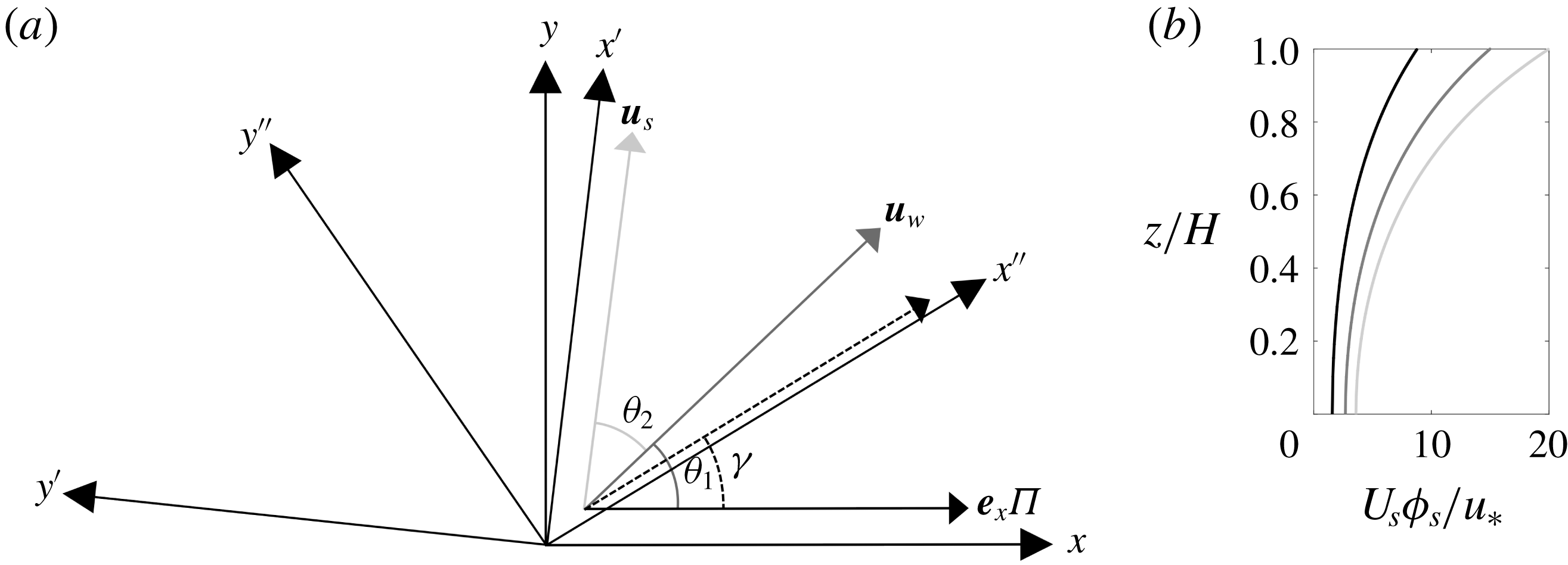
is the dominant wavenumber of surface waves (Phillips Reference Phillips1966). For scenarios in which the wind, wave and pressure-gradient forcing are coaligned – a scenario seldom expected in natural settings – equations (2.1) and (2.7) would nevertheless capture evolution of coastal Langmuir turbulence. In this article we further generalize the scope to consider arrangements in which the wind and wave forcing are aligned oblique to the column pressure gradient, as per figure 1(a), which is the second distinguishing feature of present study relative to prior articles.
Schematic of article parameters. (a) Misaligned forcing conditions. Annotations are included for the surface wind
 $\boldsymbol{u}_{w}$
, imposed at angle
 $\unicode[STIX]{x1D703}_{1}$
, and Stokes drift
 $\boldsymbol{u}_{s}$
, imposed at angle
 $\unicode[STIX]{x1D703}_{1}+\unicode[STIX]{x1D703}_{2}$
. Mean current,
 $\boldsymbol{e}_{x}\unicode[STIX]{x1D6F1}$
, is always aligned with
 $x$
direction. Through systematic variation of parameters (case details summarized in table 1), we have recovered the resultant Langmuir cell inclination,
 $\unicode[STIX]{x1D6FE}$
, for each case. In addition to Cartesian coordinate system used for LES, we also include the local coordinates,
 $\{x^{\prime },y^{\prime },z\}$
and
 $\{x^{\prime \prime },y^{\prime \prime },z\}$
, where the former and latter are aligned with the Stokes drift and resultant Langmuir cells, respectively. (b) Vertical profiles of the Stokes drift (2.12), aligned in the
 $x^{\prime \prime }$
direction, for
 $\unicode[STIX]{x1D6F9}_{2}=8.8$
(black), 15 (grey) and 20 (light grey), which correspond to cases
 $C_{1211}$
,
 $C_{2211}$
and
 $C_{3211}$
, respectively, summarized in table 1. This panel provides perspective on the magnitude of the Stokes drift magnitude, when viewed in a plane parallel with
 $\boldsymbol{u}_{s}$
.

Figure 1(a) is a planform view of the horizontal coordinates,
 $x$
and
 $y$
, with annotations for imposed pressure-gradient forcing (always aligned with
 $x$
in the present study), the prevailing atmospheric wind stress (imposed at angle
 $\unicode[STIX]{x1D703}_{1}$
) and the Stokes drift vector (imposed at angle
 $\unicode[STIX]{x1D703}_{1}+\unicode[STIX]{x1D703}_{2}$
). With this, the vortex forcing in (2.7) exhibits a different form:
 $$\begin{eqnarray}\displaystyle \boldsymbol{f}^{\unicode[STIX]{x1D714}}=u_{s,y}(\unicode[STIX]{x2202}_{x}\tilde{v}-\unicode[STIX]{x2202}_{y}\tilde{u} )\hat{i} -u_{s,x}(\unicode[STIX]{x2202}_{x}\tilde{v}-\unicode[STIX]{x2202}_{y}\tilde{u} ){\hat{j}}+[u_{s,x}(\unicode[STIX]{x2202}_{z}\tilde{u} -\unicode[STIX]{x2202}_{x}\tilde{w})-u_{s,y}(\unicode[STIX]{x2202}_{y}\tilde{w}-\unicode[STIX]{x2202}_{z}\tilde{v})]\hat{k}, & & \displaystyle\end{eqnarray}$$
where the vorticity terms have been substituted, while terms multiplied by
 $u_{s,z}$
immediately vanish since the vertical component of the Stokes drift vector is always zero. In fact, readers will immediately recognize that under the standard, aligned conditions,
 $u_{s,y}$
is also zero, thus defaulting (2.11) to the standard arrangement in which a spanwise and vertical force sustain the Langmuir cells (i.e. (2.3)). With (2.11), it is thus necessary to define the
 $y$
component of the Stokes drift, which is
 $$\begin{eqnarray}\displaystyle \boldsymbol{u}_{s}=\unicode[STIX]{x1D719}_{s}(z)\cos (\unicode[STIX]{x1D703}_{1}+\unicode[STIX]{x1D703}_{2})\hat{i} +\unicode[STIX]{x1D719}_{s}(z)\sin (\unicode[STIX]{x1D703}_{1}+\unicode[STIX]{x1D703}_{2})~{\hat{j}}+0\hat{k}, & & \displaystyle\end{eqnarray}$$
where
 $\unicode[STIX]{x1D719}_{s}(z)$
has been defined with (2.12). Equation (2.11) can thus be restated once more, as
 $$\begin{eqnarray}\displaystyle \boldsymbol{f}^{\unicode[STIX]{x1D714}} & = & \displaystyle \unicode[STIX]{x1D719}_{s}(z)\sin (\unicode[STIX]{x1D703}_{1}+\unicode[STIX]{x1D703}_{2})(\unicode[STIX]{x2202}_{x}\tilde{v}-\unicode[STIX]{x2202}_{y}\tilde{u} )\hat{i} -\unicode[STIX]{x1D719}_{s}(z)\cos (\unicode[STIX]{x1D703}_{1}+\unicode[STIX]{x1D703}_{2})(\unicode[STIX]{x2202}_{x}\tilde{v}-\unicode[STIX]{x2202}_{y}\tilde{u} ){\hat{j}}\nonumber\\ \displaystyle & & \displaystyle +\,\unicode[STIX]{x1D719}_{s}(z)[\cos (\unicode[STIX]{x1D703}_{1}+\unicode[STIX]{x1D703}_{2})(\unicode[STIX]{x2202}_{z}\tilde{u} -\unicode[STIX]{x2202}_{x}\tilde{w})-\sin (\unicode[STIX]{x1D703}_{1}+\unicode[STIX]{x1D703}_{2})(\unicode[STIX]{x2202}_{y}\tilde{w}-\unicode[STIX]{x2202}_{z}\tilde{v})]\hat{k}.\end{eqnarray}$$
By imposing the presence of oblique wave forcing, we can nevertheless use the underlying vortex forcing form to develop an
 $x$
-component forcing, as is seen in (2.13). Figure 1(b) shows the Stokes drift profiles in the
 $x^{\prime }$
–
 $z$
plane (i.e. aligned in the direction of maximum Stokes shear; see also figure 1
a).
Quick inspection of (2.13) shows that for ideal cases with all forcing aligned in the primary transport direction (tentatively the streamwise direction,
 $x$
),
 $\unicode[STIX]{x1D703}_{1}=\unicode[STIX]{x1D703}_{2}=0$
, resulting in
 $\sin (\unicode[STIX]{x1D703}_{1}+\unicode[STIX]{x1D703}_{2})=0$
and
 $\cos (\unicode[STIX]{x1D703}_{1}+\unicode[STIX]{x1D703}_{2})=1$
, and recovery of the ‘standard’ vortex forcing conditions (i.e. (2.3), but for a coastal-zone Stokes drift profile,
 $\unicode[STIX]{x1D719}_{s}(z)$
). Here, the Stokes drift surface velocity is
 $U_{s}=f_{w}ka^{2}\coth kH$
, where
 $f_{w}=(gk\tanh kH)^{1/2}$
is the frequency,
 $k=2\unicode[STIX]{x03C0}/\unicode[STIX]{x1D6EC}$
is the dominant wavenumber, where
 $\unicode[STIX]{x1D6EC}$
corresponds to the dominant wavelength, and
 $a$
is the dominant amplitude of surface waves (see Gargett & Wells (Reference Gargett and Wells2007) for calculation of these wave characteristics from field measurements).
The introduction of
 $\unicode[STIX]{x1D6F9}_{1}$
and
 $\unicode[STIX]{x1D6F9}_{2}$
is necessary since we have the additional complexity of
 $u_{\ast }$
(similar to Martinat et al.
Reference Martinat, Xu, Grosch and Tejada-Martínez2011; Gargett & Grosch Reference Gargett and Grosch2014; Shrestha et al.
Reference Shrestha, Anderson and Kuehl2018). These ratios enable quantification of the aggregate shearing due to simultaneous top and bottom drag, and are thus appropriate for the present article. In subsequent sections, we will define
 $\unicode[STIX]{x1D6F9}_{1}$
and
 $\unicode[STIX]{x1D6F9}_{2}$
for different simulations, and it is emphasized that the parameters are always based on the magnitudes and not the value of Stokes drift or wind drag in a certain direction.
In this article, we wish to explore how the OML and, in particular, the alignment of Langmuir cells,
 $\unicode[STIX]{x1D6FE}$
, vary with changes to what are presumed to be the dependent parameters,
 $\unicode[STIX]{x1D6F9}_{1}$
,
 $\unicode[STIX]{x1D6F9}_{2}$
,
 $\unicode[STIX]{x1D703}_{1}$
and
 $\unicode[STIX]{x1D703}_{2}$
(see also figure 1
a). That is, we wish to define the function
 $$\begin{eqnarray}\displaystyle \unicode[STIX]{x1D6FE}=\unicode[STIX]{x1D6FE}(\unicode[STIX]{x1D6F9}_{1},\unicode[STIX]{x1D6F9}_{2},\unicode[STIX]{x1D703}_{1},\unicode[STIX]{x1D703}_{2}). & & \displaystyle\end{eqnarray}$$
To our knowledge, theoretical deduction is not possible, rendering rigorous parametric assessment the only plausible approach. This variation of parameters will enable recovery of the resultant streamwise obliquity of Langmuir cells,
 $\unicode[STIX]{x1D6FE}$
, as per figure 1. In §§ 2.3 and 2.4, we provide information on the obliquely forced Langmuir turbulence cases considered in this study.
During numerical integration of the transport equations, an incompressible flow is maintained by computing the divergence of (2.7) and imposing (2.1), which yields a Poisson equation of dynamic pressure. Solution of this Poisson equation results in the pressure correction, which preserves (2.1). By virtue of spectral discretization in the horizontal directions, periodic boundary conditions are applied on vertical faces of the domain. The top domain boundary condition is imposed with a constant aerodynamic surface stress, which captures imposed atmospheric drag:
 $$\begin{eqnarray}\displaystyle \unicode[STIX]{x1D70F}_{iz,w}=\unicode[STIX]{x1D70F}_{w}\hat{n}_{i,w}=\{\unicode[STIX]{x1D70F}_{w}\cos \unicode[STIX]{x1D703}_{1},\unicode[STIX]{x1D70F}_{w}\sin \unicode[STIX]{x1D703}_{1}\}, & & \displaystyle\end{eqnarray}$$
where
 $\unicode[STIX]{x1D70F}_{w}$
is the ambient imposed atmospheric stress and
 $\hat{n}_{i,w}$
is a unit vector representing the constituent magnitudes of stress based on aloft winds. Herein, for simplicity, we instead decompose the imposed stress via the obliquity angle,
 $\unicode[STIX]{x1D703}_{1}$
, which is shown in figure 1(a). In addition, we impose the non-penetration condition for vertical velocity,
 $\tilde{w}|_{z/H=1}=0$
. A localized version of the logarithmic equilibrium wall model is implemented for the bottom-boundary-layer hydrodynamic stress (see details in Shrestha et al.
Reference Shrestha, Anderson and Kuehl2018):
 $$\begin{eqnarray}\displaystyle {\displaystyle \frac{\unicode[STIX]{x1D70F}_{iz,\ast }(x,y,t)}{\unicode[STIX]{x1D70C}}}=\left[{\displaystyle \frac{\unicode[STIX]{x1D705}U(x,y,z,t)}{\log (z/z_{0})}}\right]^{2}{\displaystyle \frac{\widehat{\tilde{u} }_{i}(x,y,z,t)}{U(x,y,z,t)}},\quad i=1,2, & & \displaystyle\end{eqnarray}$$
where
 $U(x,y,z,t)$
is the local magnitude of the test-filtered velocity, which is denoted by
 $\widehat{\tilde{\ldots }}$
in (2.16) (Meneveau & Katz Reference Meneveau and Katz2000; Pope Reference Pope2000; Bou-Zeid, Meneveau & Parlange Reference Bou-Zeid, Meneveau and Parlange2005; Anderson & Meneveau Reference Anderson and Meneveau2011). This ‘local’ application of the logarithmic law for bed stress is necessitated during wall-modelled LES, which is a necessary condition for closure of the system (Pope Reference Pope2000). We recognize that conditions in the bottom boundary layer may diverge sharply from logarithmic scale, which may undermine the simulations by deployment of a logarithmic stress model. To this extent, we contend that the logarithmic model should be viewed as a means to define a transfer function for momentum fluxes, i.e.
 $C_{m}(z)=-[\unicode[STIX]{x1D705}/\log (z/z_{0})]^{2}$
, where
 $z_{0}/H=10^{-2}$
is the predefined surface roughness length for the seafloor undulations (in this work, our treatment of ‘coastal zones’ encompasses only those regions wherein bathymetric spatial undulations are negligible) and
 $\unicode[STIX]{x1D705}=0.4$
is the von Kármán constant. Deng et al. (Reference Deng, Yang, Xuan and Shen2019) have presented evidence that the disrupted logarithmic layer reported at lower Reynolds number reappears at high Reynolds number (Tejada-Martínez et al.
Reference Tejada-Martínez, Grosch, Sinha, Akan and Martinat2012).
Centred, second-order finite differencing is used to evaluate vertical gradients, and the second-order Adams–Bashforth scheme has been used for time integration. The nonlinear advective term is dealiased with the
 $3/2$
rule (Orszag Reference Orszag1970). Note that in this article, averaging of test quantity,
 $\unicode[STIX]{x1D703}(a)$
, over its independent dimension,
 $a$
, is denoted by
 $\langle \unicode[STIX]{x1D703}\rangle _{a}$
. Reynolds averaging is denoted by
 $\langle \ldots \rangle _{T}$
; Reynolds-averaged quantities presented herein are based upon averaging over
 $TU_{0}H^{-1}=91$
large-eddy turnovers, and averaging is not performed until the flow attains equilibrium with the imposed forcing. The LES code is an extension of the Johns Hopkins University LES code (Albertson & Parlange Reference Albertson and Parlange1999; Bou-Zeid et al.
Reference Bou-Zeid, Meneveau and Parlange2005), with generalizations made to capture coastal-zone Langmuir turbulence (Shrestha et al.
Reference Shrestha, Anderson and Kuehl2018). The code has been used for nearly two decades to study a diverse range of inertia-dominated geophysical shear flows (Bou-Zeid et al.
Reference Bou-Zeid, Meneveau and Parlange2005; Anderson & Meneveau Reference Anderson and Meneveau2011; Graham & Meneveau Reference Graham and Meneveau2012). In a recent article (Shrestha et al.
Reference Shrestha, Anderson and Kuehl2018), we demonstrated the efficacy of the code for modelling the OML relative to benchmark datasets in the literature (McWilliams et al.
Reference McWilliams, Sullivan and Moeng1997).
2.3 Base flow set-up
For this study, we have considered the inclusion of a mean current forcing – designed to capture the modulation of Langmuir turbulence by tides or by larger-scale circulation, for example those associated with the Gulf of Mexico’s Loop Current and associated shed eddies impinging upon the coastal zones (DiMarco, Howard & Reid Reference DiMarco, Howard and Reid2000; Oye, Ezer & Lee Reference Oye, Ezer and Lee2005; Lipphardt et al.
Reference Lipphardt, Poje, Kirwan, Kantha and Zweng2008; Kuehl & Sheremet Reference Kuehl and Sheremet2014; Kuehl et al.
Reference Kuehl, DiMarco, Spencer and Guinasso2014; Spencer et al.
Reference Spencer, DiMarco, Wang, Kuehl and Brooks2016) – in LES of Langmuir turbulence. The majority of the monochromatic surface wave parameters are based on field observation data recovered from shallow, coastal zones (i.e.
 $H=15~\text{m}$
water depth) in the shelf coastal region of New Jersey (Gargett et al.
Reference Gargett, Wells, Tejada-Martínez and Grosch2004; Gargett & Wells Reference Gargett and Wells2007, their ‘Record 43.025’). The computational domain is a rectangular prism;
 $L_{x}=L_{y}=2\unicode[STIX]{x03C0}H$
, with depth,
 $H=15~\text{m}$
, with
 $[192\times 192\times 192]$
grid points used for the computational resolution. The domain size is smaller than used in comparable prior studies, for example Tejada-Martínez & Grosch (Reference Tejada-Martínez and Grosch2007). However, we also note that a recent article by Shrestha et al. (Reference Shrestha, Anderson and Kuehl2018) performed dynamically equivalent simulations with domains of different sizes, and found no size dependence. The present LES code has been used for many years to model inertia-dominated turbulent channel flows (and subset problems, such as the present application to coastal Langmuir turbulence), and in preceding work no resolution sensitivity has been reported (Bou-Zeid et al.
Reference Bou-Zeid, Meneveau and Parlange2005; Anderson & Meneveau Reference Anderson and Meneveau2011; Stevens, Wilczek & Meneveau Reference Stevens, Wilczek and Meneveau2014). The LES computational mesh resolution is uniform in all directions, and thus no grid refinement predicated upon local shear is possible (some use near-wall refinement to enhance resolution of the associated elevated mixing, but herein we assume that the subgrid-scale treatment sufficiently captures the effects of elevated near-wall processes). We prescribe
 $u_{w}=3.22\times 10^{-3}~\text{m}~\text{s}^{-1}$
. With these values, we estimate a shear Reynolds number,
 $R_{w}=u_{w}H/\unicode[STIX]{x1D708}\sim O(10^{4})$
. This very large
 $Re_{\ast }$
provides overwhelming support for treatment of coastal-zone Langmuir turbulence as a ‘fully rough’ phenomenon, which underpins the study in two ways: (i) this
 $Re_{\ast }$
justifies omission of the viscous stress tensor in (2.2) and (ii) ‘fully rough’ mixing enables comparison of LES and field results under the existence of dynamic similarity (inertia-dominated mixing). In the interest of brevity, we have not included results of sensitivity testing of resolution or grid aspect ratio, since we performed such testing in a very recent article (Shrestha et al.
Reference Shrestha, Anderson and Kuehl2018).
The base case with coaligned wind, wave and mean current forcing (i.e.
 $\unicode[STIX]{x1D703}_{1}=\unicode[STIX]{x1D703}_{2}=0$
in figure 1) has a constant wind stress,
 $\unicode[STIX]{x1D70F}_{w}=0.01~\text{N}~\text{m}^{-2}$
, on the top boundary of the shallow water column. Surface waves are characterized by frequency,
 $f_{w}=0.82~\text{rad}~\text{s}^{-1}$
; amplitude,
 $a=0.67~\text{m}$
; wavenumber,
 $k=0.08~\text{rad}~\text{m}^{-1}$
corresponding to wavelength
 $\unicode[STIX]{x1D6EC}=79~\text{m}$
(
 $\unicode[STIX]{x1D6EC}/H=5.26$
); and Stokes drift surface velocity,
 $U_{s}=0.036~\text{m}~\text{s}^{-1}$
. As per (2.5), these values result in
 $La_{t}=0.3$
, and non-dimensional wavenumber,
 $kH=1.2$
. Since the mean current force is imposed in the LES via pressure gradient,
 $\boldsymbol{e}_{x}\unicode[STIX]{x1D6F1}$
, calculations yield a mean current speed,
 $U_{c}=1.27~\text{m}~\text{s}^{-1}$
, using the relation
 $\unicode[STIX]{x1D70F}_{\ast }=\unicode[STIX]{x1D70C}C_{d}U_{c}^{2}$
, where
 $C_{d}=2.5\times 10^{-3}$
is a candidate value for the drag coefficient (Sternberg Reference Sternberg1968; Sherwood, Lacey & Voulgaris Reference Sherwood, Lacey and Voulgaris2006),
 $\unicode[STIX]{x1D70F}_{\ast }$
is the bottom-boundary-layer surface stress and
 $U_{c}$
is a mean current velocity due to the ‘Loop Current ring’, shed from the Loop Current. The value of
 $U_{c}=1.27~\text{m}~\text{s}^{-1}$
falls within the range (peak speed
 ${\sim}1.8~\text{m}~\text{s}^{-1}$
) observed by Oye et al. (Reference Oye, Ezer and Lee2005). The
 $u_{\ast }$
-normalized Stokes drift magnitude and atmospheric shear velocity have already been defined with (2.8) and (2.9), respectively (Martinat et al.
Reference Martinat, Xu, Grosch and Tejada-Martínez2011; Gargett & Grosch Reference Gargett and Grosch2014). The flow is presumed to exist under high-Rossby-number conditions, thereby eliminating the need to consider Corilois accelerations during integration of (2.2). Moreover, thermal gradients are presumed to have been homogenized by ambient, shear-driven mixing, and for this reason no vertical buoyancy flux is included during numerical integration of (2.2). These conditions are supported by field observations (Gargett et al.
Reference Gargett, Wells, Tejada-Martínez and Grosch2004; Gargett & Wells Reference Gargett and Wells2007), and are consistent with preceding numerical studies of coastal-zone Langmuir turbulence (Tejada-Martínez & Grosch Reference Tejada-Martínez and Grosch2007; Kukulka, Pleuddemann & Sullivan Reference Kukulka, Pleuddemann and Sullivan2012; Shrestha et al.
Reference Shrestha, Anderson and Kuehl2018).
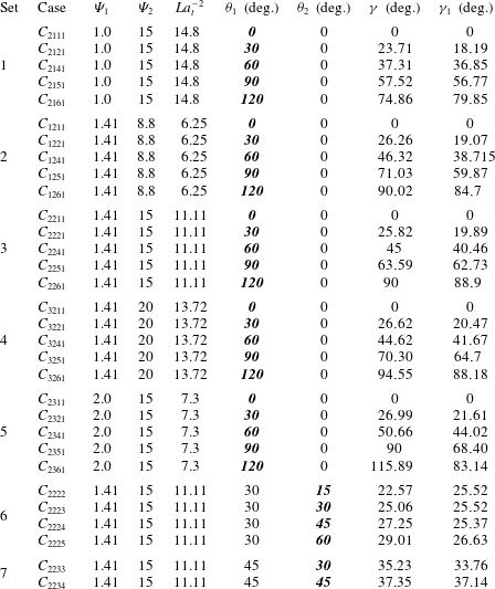
Summary of forcing conditions and cases studied for this article (see also (2.14) and accompanying text). The simulation campaign is composed of seven distinct sets, where each set was designed to isolate the role of a single dependent parameter. The simulations address the full parameter space –
 $\unicode[STIX]{x1D6F9}_{1}$
,
 $\unicode[STIX]{x1D6F9}_{2}$
,
 $\unicode[STIX]{x1D703}_{1}$
and
 $\unicode[STIX]{x1D703}_{2}$
– through systematic variation of forcing magnitude and obliquity relative to the ambient, streamwise pressure-gradient forcing. Here
 $\unicode[STIX]{x1D6FE}$
is the orientation of resultant Langmuir cells (see also figure 1
a) and is derived from the spatial correlation map of fluctuating resolved spanwise velocity,
 $\unicode[STIX]{x1D70C}_{\tilde{v}^{\prime }\tilde{v}^{\prime }}$
(3.1). As part of this work, prognostic models for
 $\unicode[STIX]{x1D6FE}$
have been developed, and output values from a prognostic model are summarized in the table (
 $\unicode[STIX]{x1D6FE}_{1}$
, equation (3.5)). In order to isolate the dependence of
 $\unicode[STIX]{x1D6FE}$
upon its dependent parameters, 29 discrete cases were selected, where case is denoted by
 $C_{ijpq}$
, where the indices denote the case. In the table, parameters in bold and italics are being varied, while
 $i=1$
, 2 and 3 correspond to
 $U_{s}/u_{\ast }=8.8$
, 15 and 20, respectively;
 $j=1$
, 2 and 3 correspond to
 $u_{w}/u_{\ast }=1.0$
, 1.41 and 2.0, respectively;
 $p=1$
, 2, 3, 4, 5 and 6 correspond to
 $\unicode[STIX]{x1D703}_{1}=0^{\circ }$
,
 $30^{\circ }$
,
 $45^{\circ }$
,
 $60^{\circ }$
,
 $90^{\circ }$
and
 $120^{\circ }$
;
 $q=1$
, 2, 3, 4 and 5 correspond to
 $\unicode[STIX]{x1D703}_{2}=0^{\circ }$
,
 $15^{\circ }$
,
 $30^{\circ }$
,
 $45^{\circ }$
and
 $60^{\circ }$
, respectively.

2.4 Misalignment cases
The effects of misaligned wind, wave and mean current forcing are studied through different case set-ups of varying forcing parameters and misalignment angles, as summarized in table 1. The angles (
 $\unicode[STIX]{x1D703}_{1}$
,
 $\unicode[STIX]{x1D703}_{2}$
and
 $\unicode[STIX]{x1D6FE}$
) are summarized in table 1, and are graphically displayed in figure 1(a). This study is based on the assumption that the resultant Langmuir cell orientation is affected by the magnitude of underlying forcing parameters and their directional misalignment. For a systematic study of the role of each parameter in defining
 $\unicode[STIX]{x1D6FE}$
, different simulation cases are selected such that the role of dependent parameters can be thoroughly isolated. In this regard, a series of simulation cases is uniquely identified by the given case nomenclature,
 $C_{ijpq}$
, where the indices vary as shown in table 1. In the nomenclature,
 $C$
denotes ‘coastal’ conditions, while
 $i=1$
to 3 (i.e. three values of
 $U_{s}/u_{\ast }$
),
 $j=1$
to 3 (i.e. three values of
 $u_{w}/u_{\ast }$
),
 $p=1$
to 6 (i.e. six values of
 $\unicode[STIX]{x1D703}_{1}$
) and
 $q=1$
to 5 (i.e. five values of
 $\unicode[STIX]{x1D703}_{2}$
). We have established that this range of parameters is sufficient to identify the dependence – and the hierarchical dependence – of
 $\unicode[STIX]{x1D6FE}$
upon dependent parameters.
The study may be interpreted as being composed of seven sets of simulations, where each set has been highlighted in table 1 and is itself composed of a series of cases; the table has been prepared such that the dependent parameter being varied is in bold and italics. The influence of
 $\unicode[STIX]{x1D703}_{1}$
is tested in Sets 1 to 5, for varying
 $\unicode[STIX]{x1D6F9}_{2}$
(Sets 2, 3 and 4), and varying
 $\unicode[STIX]{x1D6F9}_{1}$
(Sets 1 and 5). The magnitude ranges,
 $8.8\leqslant \unicode[STIX]{x1D6F9}_{2}\leqslant 20$
and
 $1.0\leqslant \unicode[STIX]{x1D6F9}_{1}\leqslant 2.0$
, are within ‘typical’ coastal values (Gargett et al.
Reference Gargett, Wells, Tejada-Martínez and Grosch2004; Gargett & Wells Reference Gargett and Wells2007; Kukulka et al.
Reference Kukulka, Pleuddemann, Trowbridge and Sullivan2011; Martinat et al.
Reference Martinat, Xu, Grosch and Tejada-Martínez2011; Li et al.
Reference Li, Li, Gerbi and Song2013; Shrestha et al.
Reference Shrestha, Anderson and Kuehl2018), while the obliquity angles encompass the range of possible departures from the ‘pure’ case of
 $\unicode[STIX]{x1D703}_{1}=\unicode[STIX]{x1D703}_{2}=0$
(although these values are included, too, in order to provide context for the oblique-forcing cases).
In the simulations, the direction of mean current is fixed in the streamwise direction and the direction of Stokes drift and wind stress are varied to provide the required misalignment. It is important to note here that these misalignment cases involve forcing vectors aligned in different directions, which consequently alters the vortex forcing term in the momentum equation (2.2). A wider parameter range of external forcing conditions are tested by varying non-dimensional parameters
 $\unicode[STIX]{x1D6F9}_{1}$
(wind forcing) and
 $\unicode[STIX]{x1D6F9}_{2}$
(wave forcing), while keeping the mean current speed fixed, i.e.
 $U_{c}=1.27~\text{m}~\text{s}^{-1}$
(see also § 2.3). For context, table 1 includes corresponding values for
 $La_{t}^{-2}$
; this helps to give readers a physical intuition for the nature of the flows relative to open-ocean cases, and for the relative magnitude of
 $\unicode[STIX]{x1D6F9}_{2}$
relative to
 $La_{t}^{-2}$
.
3 Results
This section is composed of results and deductions on the changing spatial nature of coastal-zone Langmuir turbulence, as salient parameters governing the orientation are changed (i.e. equation (2.14)). The presentation of results begins with computation of the inclination angle,
 $\unicode[STIX]{x1D6FE}$
, from two-point correlation of the resolved fluctuating velocity, and implications of this for resultant hydrodynamic bed stresses. We also show sensitivity testing results on the systematic variation of salient parameters upon
 $\unicode[STIX]{x1D6FE}$
, and leverage these results to propose new prognostic closures for
 $\unicode[STIX]{x1D6FE}$
; results from the new model are compared against existing empirical models based upon Lagrangian shear (foremost among them being the contribution from Van Roekel et al. (Reference Van Roekel, Fox-Kemper, Sullivan, Hamlington and Haney2012), which was based upon open-ocean conditions, absent hydrodynamic bathymetric shear). We also show vertical profiles for first- and second-order turbulent quantities, and for constituent terms within the transport equation for turbulent kinetic energy,
 $tke$
.
3.1 Coastal-zone Langmuir cell alignment
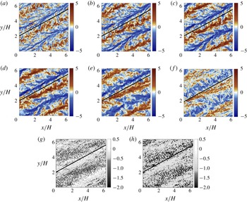
In order to provide some initial, qualitative illustration of the nature of coastal Langmuir turbulence, we show figure 2. Figure 2(a–f) shows instantaneous resolved vertical velocity,
 $\tilde{w}(x,y,z,t)/u_{\ast }$
, at depths noted in the caption, while figure 2(g,h) shows the associated bottom-bed hydrodynamic (bathymetric) stresses, as per (2.16) (see § 2.2). Results are shown for Case
 $C_{2221}$
(table 1), which corresponds to a case of coaligned wind and wave forcing and forcing magnitudes,
 $\unicode[STIX]{x1D6F9}_{1}=1.41$
and
 $\unicode[STIX]{x1D6F9}_{2}=15$
, imposed at an angle oblique to the streamwise direction. Owing to the oblique wind and wave forcing, relative to the ambient pressure-gradient forcing, the resultant Langmuir cells are also oblique to streamwise. Note, however, that the actual inclination of the cells is less than that of the wind and wave forcing, i.e.
 $\unicode[STIX]{x1D6FE}<\unicode[STIX]{x1D703}_{1}=30^{\circ }$
. This can be deduced from cursory assessment of the figures: since
 $(L/H)\tan (30^{\circ })\approx 3.5$
, one can infer that the cells are aligned at an angle less than
 $\unicode[STIX]{x1D703}_{1}$
. In the absence of a coastal pressure-gradient forcing (and bottom-bed shear), the Langmuir cells would be aligned precisely in the direction of the coaligned wind and wave forcing. But, owing to the competing influence of the bottom bed shear and wind and wave shear, the cells align themselves at an intermediate angle,
 $0\leqslant \unicode[STIX]{x1D6FE}<\unicode[STIX]{x1D703}_{1}$
. In fact, this is a recurrent result that we observe throughout the study. The concluding stages of the results section provide theoretical justification for this result.
Comparison of structural orientation of the resultant Langmuir cells for Case
 $C_{2221}$
. (a–f) Instantaneous resolved vertical velocity at column depths
 $z/H=0.9$
(a),
 $z/H=0.8$
(b),
 $z/H=0.7$
(c),
 $z/H=0.6$
(d),
 $z/H=0.4$
(e) and
 $z/H=0.2$
(f). Instantaneous hydrodynamic bed stress (g)
 $\unicode[STIX]{x1D70F}_{xz,\ast }(z,y)/u_{\ast }^{2}$
and (h)
 $\unicode[STIX]{x1D70F}_{yz,\ast }(x,y)/u_{\ast }^{2}$
(see also (2.16)). For reference, panels include line denoting the angle
 $\unicode[STIX]{x1D703}_{1}+\unicode[STIX]{x1D703}_{2}$
.

The signature of the Langmuir cells is evident in figure 2(a–f) by virtue of self-organization into rows of predominant upwelling (
 $\tilde{w}(x,y,z,t)/u_{\ast }>0$
, red) and downwelling (
 $\tilde{w}(x,y,z,t)/u_{\ast }<0$
, blue), where figures 2(a) and 2(f) correspond to horizontal planes closest to the ocean surface and seafloor, respectively. Moreover, the cells appear to be most coherent at the intermediate depths (i.e. figure 2
d or 2
e). This result is a natural consequence of the lower turbulent kinetic energy,
 $tke$
, and shear production of turbulence at mid-depths; closer to the wall or ocean surface, where hydrodynamic shear is most pronounced, the presence of vigorous mixing attenuates the largest scales of the cells. We note that the orientation of the cells does not exhibit a strong ‘spiral’ pattern over the depth of the column, and instead the angle,
 $\unicode[STIX]{x1D6FE}$
, is essentially depth-insensitive. There is a negligible spiral, which can be appreciated by the reference line in figure 2(a–h), but in general the aggregate forcing yields a coherent self-organization to Langmuir cells at angle
 $\unicode[STIX]{x1D6FE}$
. This result is general to the full range of simulations summarized in table 1, and not specific to Case
 $C_{2221}$
. Note, also, that in the absence of bottom-bed stress (i.e. open-ocean settings), the cells would be aligned precisely with the coaligned wind and wave forcing – as per the preceding results from Van Roekel et al. (Reference Van Roekel, Fox-Kemper, Sullivan, Hamlington and Haney2012) – but the presence of bottom-boundary stress induces a realignment away from
 $x^{\prime }$
, toward
 $x$
(see figure 1 for reference).
Finally, figure 2(g,h) shows the instantaneous components of hydrodynamic bed stress, as imposed during LES with (2.16). Figures 2(g) and 2(h) correspond to the streamwise-vertical and spanwise-vertical momentum fluxes, respectively, and as such correlate closely with figures 2(a–f). Within locations of downwelling, there is a relative excess of streamwise velocity, and as such the zones of elevated
 $\unicode[STIX]{x1D70F}_{xz,\ast }(x,y,t)$
correlate precisely with regions of
 $\tilde{w}<0$
. Similarly, at the base of downwelling zones, conservation of mass dictates a lateral outflow, which results in the regions of equal and opposite
 $\unicode[STIX]{x1D70F}_{yz,\ast }(x,y,t)$
in figure 2(h) (effectively, the
 $\unicode[STIX]{x1D70F}_{yz,\ast }(x,y,t)$
pattern is identical to
 $\unicode[STIX]{x1D70F}_{xz,\ast }(x,y,t)$
, but is phase shifted in the
 $y^{\prime \prime }$
direction, again due to the lateral outflow at the base of downwelling zones).
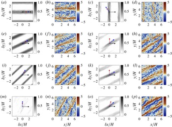
Numerical experiments on the effect of oblique wind, wave and mean current forcing. Panels (a,c,e,g,i,k,m,o) (i.e. first and third columns) show two-point correlation contour maps,
 $\unicode[STIX]{x1D70C}_{\tilde{v}^{\prime }\tilde{v}^{\prime }}(\unicode[STIX]{x1D6FF}z,\unicode[STIX]{x1D6FF}y,z)$
(3.1); superimposed upon the colour contours are coloured arrows to denote the direction of forces: red arrow indicates wave direction, blue arrow indicates wind direction and black arrow indicates mean current direction. Panels (b,d,f,h,j,l,n,p) (i.e. second and fourth columns) show instantaneous, resolved vertical velocity at column depth. For all panels, the results are shown at depth
 $z/H=0.18$
. Results are shown for table 1 cases:
 $C_{2211}$
(a,b),
 $C_{2261}$
(c,d),
 $C_{2221}$
(e,f),
 $C_{2234}$
(g,h),
 $C_{2241}$
(i,j),
 $C_{2225}$
(k,l),
 $C_{2251}$
(m,n) and
 $C_{2233}$
(o,p).

Figure 3(b,d,f,h,j,l,n,p) (i.e. the second and fourth columns of figure 3) shows instantaneous, resolved vertical velocity for cases noted in the figure caption at column depth
 $z/H=0.18$
. Figure 3(a,c,e,g,i,k,m,o) (i.e. the first and third columns of figure 3) shows the corresponding contours of two-point correlation of resolved spanwise velocity, computed as
 $$\begin{eqnarray}\displaystyle \unicode[STIX]{x1D70C}_{\tilde{v}^{\prime }\tilde{v}^{\prime }}(\unicode[STIX]{x1D6FF}x,\unicode[STIX]{x1D6FF}y,z)={\displaystyle \frac{\langle \tilde{v}^{^{\prime }}(x,y,z)\tilde{v}^{^{\prime }}(x+\unicode[STIX]{x1D6FF}x,y+\unicode[STIX]{x1D6FF}y,z)\rangle _{T}}{\unicode[STIX]{x1D70E}_{y}(z)\unicode[STIX]{x1D70E}_{y}(z)}}, & & \displaystyle\end{eqnarray}$$
where
 $\unicode[STIX]{x1D6FF}x$
and
 $\unicode[STIX]{x1D6FF}y$
are spatial separation in the streamwise and spanwise direction, respectively, and
 $\unicode[STIX]{x1D70E}_{y}$
is the root-mean-square value of resolved spanwise velocity. Spanwise velocity provided the most clarity on cell orientation. The time averaging spans
 ${\approx}10^{2}$
large-eddy turnovers after the turbulence statistics have become stationary. Fluctuations are based upon subtraction of a plane average – where spatial undulation of the Langmuir cells is presumed to impose a modest influence relative to the remaining turbulent fluctuations, thereby enabling the assumption of horizontal homogeneity for the purpose of computing turbulence statistics. In testing performed during preparation of this article, we found that the cells exhibit a negligible ‘spiral’ in the vertical direction (results omitted for brevity), and thus the results at
 $z/H=0.18$
are representative of the entire column. The original directions of constant wind, monochromatic surface wave and constant mean current are shown with blue, red and black arrows, respectively (this can be cast against the figure 1(a) results, which show the local coordinate systems,
 $\{x^{\prime },y^{\prime },z\}$
and
 $\{x^{\prime \prime },y^{\prime \prime },z\}$
). Note that periodicity is observed for the local maxima and minima in the correlation map of spanwise velocity fluctuation, owing to the characteristic convergence and divergence zones of Langmuir turbulence that increases the strength of spanwise velocity (Leonardi et al.
Reference Leonardi, Orlandi, Djenidi and Antonia2004; Tejada-Martínez & Grosch Reference Tejada-Martínez and Grosch2007). It can be understood that the local maxima are separated by the distance between consecutive downwelling limbs between adjacent Langmuir cells.
Characterization of Langmuir cell orientation (i.e. deduction of resultant angle
 $\unicode[STIX]{x1D6FE}$
) is assessed by datafit of a linear ‘best fit’ profile to the two-point correlation contours, where the
 $\unicode[STIX]{x1D6FE}$
values are summarized in table 1. As expected, in all cases the resultant
 $\unicode[STIX]{x1D6FE}$
is intermediate to the combined wind, wave and pressure-gradient forcing. The correlation contours agree closely with the instantaneous visualizations, although we emphasize that
 $\unicode[STIX]{x1D70C}_{\tilde{v}^{\prime }\tilde{v}^{\prime }}(\unicode[STIX]{x1D6FF}x,\unicode[STIX]{x1D6FF}y,z)$
is predicated upon a Reynolds average while the visualizations are instantaneous. The Langmuir cells are transient in nature – their intensity varies, and they undulate in the
 $y^{\prime \prime }$
direction (see figure 1
a) – but a coherent signature can still be attained from
 $\unicode[STIX]{x1D70C}_{\tilde{v}^{\prime }\tilde{v}^{\prime }}(\unicode[STIX]{x1D6FF}x,\unicode[STIX]{x1D6FF}y,z)$
.
Note, finally, that measures of coherence demonstrate an attenuation in the coherence of the Langmuir cells with changing obliquity. Consider, for example, a measure of the integral length based upon integration in the resultant cell direction:
 $$\begin{eqnarray}\displaystyle \unicode[STIX]{x1D706}(z)=\int _{-\infty }^{\infty }\unicode[STIX]{x1D70C}_{\tilde{v}^{\prime }\tilde{v}^{\prime }}(x^{\prime \prime },0,z)\,\text{d}x^{\prime \prime }, & & \displaystyle\end{eqnarray}$$
where the two-point correlation has been mapped into the
 $\{x^{\prime \prime },y^{\prime \prime },z\}$
coordinate system. It is clear that for Cases
 $C_{2211}$
(figure 3
a,b),
 $C_{2261}$
(figure 3
e,f) and
 $C_{2221}$
(figure 3
i,j) – that is, cases for which the wind and wave forces are coaligned, and not normal to the streamwise direction – the coherence is strongest and, thus,
 $\unicode[STIX]{x1D706}(z)$
would be greatest. In contrast, when the wind and wave forcing is imposed at an angle normal (Case
 $C_{2251}$
, figure 3
m,n) or greater than normal (Case
 $C_{2261}$
, figure 3
c,d), or when the wind and wave forcing is not coaligned (Cases
 $C_{2234}$
,
 $C_{2225}$
and
 $C_{2233}$
, shown in figures 3
g,h, 3
k,l and 3
o,p, respectively), the correlation weakens. Even when the cell coherence is weakest – for example, Case
 $C_{2251}$
(figure 3
m,n) – some record of Langmuir cells is nevertheless present. Although the focus of this article is deduction of the resultant angle,
 $\unicode[STIX]{x1D6FE}$
, for variable coastal forcing conditions, it is notable that the self-organization process leading to Langmuir cells is robust for such complex conditions.
Development of prognostic models for a priori prediction of resultant Langmuir cell orientation angle is a major component of this work. In § 3.1, we showed how this angle varied for a range of cases (figure 3 and accompanying text), while table 1 includes
 $\unicode[STIX]{x1D6FE}$
from all the cases considered in this article. Fundamentally, the production and sustenance of Langmuir circulations are associated with the tilting of spanwise and vertical vorticity by Lagrangian shear and, thus, the resultant cells must be aligned with the direction of mean Lagrangian shear. As a preliminary effort, we consider an a priori prediction model involving wind, wave and mean current, inspired by the model developed by Van Roekel et al. (Reference Van Roekel, Fox-Kemper, Sullivan, Hamlington and Haney2012). They considered the scenario of wind and wave forcing in open-ocean conditions, with the wind directed in the streamwise direction; their model for resultant Langmuir cell orientation,
 $\unicode[STIX]{x1D6FC}$
, is
 $$\begin{eqnarray}\displaystyle \unicode[STIX]{x1D6FC}=\arctan \left({\displaystyle \frac{\left\langle {\displaystyle \frac{\text{d}v_{s}}{\text{d}z}}\right\rangle _{z}}{\left\langle {\displaystyle \frac{\text{d}u_{s}}{\text{d}z}}\right\rangle _{z}+\left\langle {\displaystyle \frac{\text{d}u|_{w}}{\text{d}z}}\right\rangle _{z}}}\right), & & \displaystyle\end{eqnarray}$$
where
 $u_{s}$
and
 $v_{s}$
are the horizontal components of Stokes drift,
 $u|_{w}$
is the streamwise velocity profile due to the imposed wind shear (approximated by the law of wall) and
 $\langle \rangle _{z}$
denotes vertical averaging from the surface to twice the e-folding depth of the Stokes drift.
The present coastal ocean context is a generalized scenario of the above, for which the mean current forcing affects the dynamics and the resultant cell alignment. However, since shear is the underlying driver of Langmuir cell intensity and generation, it is self-evident that the arguments upon which (3.3) were developed are also valid in coastal settings. To this extent, equation (3.3) can be reformulated to obtain resultant coastal-zone Langmuir cell orientation angle,
 $\unicode[STIX]{x1D6FE}_{1}$
, as follows:
 $$\begin{eqnarray}\displaystyle \unicode[STIX]{x1D6FE}_{1}=\arctan \left({\displaystyle \frac{\left\langle {\displaystyle \frac{\text{d}v_{s}}{\text{d}z}}\right\rangle _{z}+\left\langle {\displaystyle \frac{\text{d}v|_{w}}{\text{d}z}}\right\rangle _{z}}{\left\langle {\displaystyle \frac{\text{d}u_{s}}{\text{d}z}}\right\rangle _{z}+\left\langle {\displaystyle \frac{\text{d}u|_{w}}{\text{d}z}}\right\rangle _{z}+\left\langle {\displaystyle \frac{\text{d}u_{b}}{\text{d}z}}\right\rangle _{z}}}\right), & & \displaystyle\end{eqnarray}$$
where
 $\text{d}u|_{w}/\text{d}z$
and
 $\text{d}v|_{w}/\text{d}z$
are the horizontal components of the Eulerian shear induced by surface wind shear – again defined here with the logarithmic law for the purpose of developing a prognostic model – and
 $\text{d}u_{b}/\text{d}z$
is the Eulerian shear induced by the mean current (also defined with the logarithmic law). It is to be noted here that the direction of the mean current is fixed in the streamwise direction and the direction of the wind and wave varies. Substitution of the definitions of the Stokes drift profile (2.12) and parameters
 $\unicode[STIX]{x1D6F9}_{1}$
and
 $\unicode[STIX]{x1D6F9}_{2}$
(2.8) and (2.9) yields the reduced form of (3.4):
 $$\begin{eqnarray}\displaystyle \unicode[STIX]{x1D6FE}_{1}=\left\{\begin{array}{@{}ll@{}}\arctan (\unicode[STIX]{x1D712})\quad & \text{for }\unicode[STIX]{x1D712}>0,\\ \unicode[STIX]{x03C0}+\arctan (\unicode[STIX]{x1D712})\quad & \text{for }\unicode[STIX]{x1D712}\leqslant 0,\end{array}\right. & & \displaystyle\end{eqnarray}$$
where substitution of terms yields the definition for
 $\unicode[STIX]{x1D712}$
 $$\begin{eqnarray}\displaystyle \unicode[STIX]{x1D712}={\displaystyle \frac{{\displaystyle \frac{\unicode[STIX]{x1D6F9}_{2}\unicode[STIX]{x1D705}}{\langle z^{-1}\rangle _{z}}}\left\langle {\displaystyle \frac{\text{d}\unicode[STIX]{x1D719}_{s}(z)}{\text{d}z}}\right\rangle _{z}\sin (\unicode[STIX]{x1D703}_{1}+\unicode[STIX]{x1D703}_{2})+\unicode[STIX]{x1D6F9}_{1}\sin (\unicode[STIX]{x1D703}_{1})}{{\displaystyle \frac{\unicode[STIX]{x1D6F9}_{2}\unicode[STIX]{x1D705}}{\langle z^{-1}\rangle _{z}}}\left\langle {\displaystyle \frac{\text{d}\unicode[STIX]{x1D719}_{s}(z)}{\text{d}z}}\right\rangle _{z}\cos (\unicode[STIX]{x1D703}_{1}+\unicode[STIX]{x1D703}_{2})+\unicode[STIX]{x1D6F9}_{1}\cos (\unicode[STIX]{x1D703}_{1})+1}}, & & \displaystyle\end{eqnarray}$$
where
 $$\begin{eqnarray}\displaystyle & \displaystyle {\displaystyle \frac{\text{d}u_{s}}{\text{d}z}}=\cos (\unicode[STIX]{x1D703}_{1}+\unicode[STIX]{x1D703}_{2}){\displaystyle \frac{\text{d}\unicode[STIX]{x1D719}_{s}(z)}{\text{d}z}},\quad {\displaystyle \frac{\text{d}v_{s}}{\text{d}z}}=\sin (\unicode[STIX]{x1D703}_{1}+\unicode[STIX]{x1D703}_{2}){\displaystyle \frac{\text{d}\unicode[STIX]{x1D719}_{s}(z)}{\text{d}z}}, & \displaystyle\end{eqnarray}$$
 $$\begin{eqnarray}\displaystyle {\displaystyle \frac{\text{d}u|_{w}}{\text{d}z}}={\displaystyle \frac{u_{w}}{\unicode[STIX]{x1D705}z}}\cos (\unicode[STIX]{x1D703}_{1}),\quad {\displaystyle \frac{\text{d}v|_{w}}{\text{d}z}}={\displaystyle \frac{u_{w}}{\unicode[STIX]{x1D705}z}}\sin (\unicode[STIX]{x1D703}_{1}) & & \displaystyle\end{eqnarray}$$
and
 $$\begin{eqnarray}\displaystyle {\displaystyle \frac{\text{d}u_{b}}{\text{d}z}}={\displaystyle \frac{u_{\ast }}{\unicode[STIX]{x1D705}z}}. & & \displaystyle\end{eqnarray}$$
Substitution of the gradients summarized in (3.7), (3.8) and (3.9), and modest algebra, yields (3.6). The development leading to (3.6) is predicated upon the assumption of logarithmic scaling due to imposed aerodynamic shear, and we must emphasize that this differs from numerical treatment of this boundary within the LES code (see § 2.2).
Study of the dependence of resultant Langmuir cell orientation,
 $\unicode[STIX]{x1D6FE}$
, on parameters
 $\unicode[STIX]{x1D6F9}_{1}$
,
 $\unicode[STIX]{x1D6F9}_{2}$
,
 $\unicode[STIX]{x1D703}_{1}$
and
 $\unicode[STIX]{x1D703}_{2}$
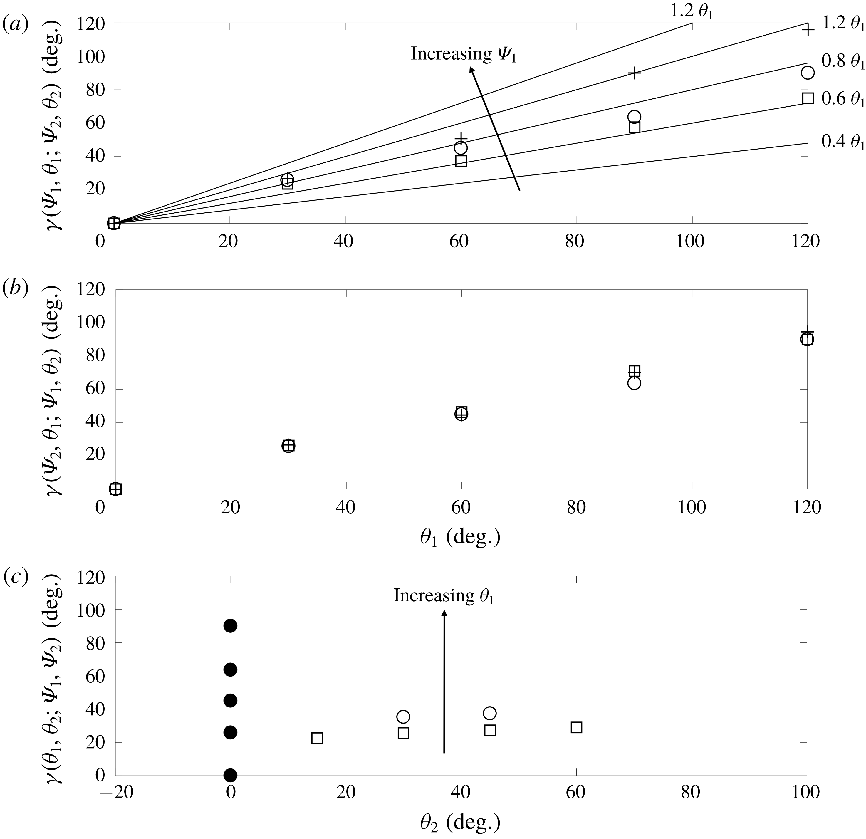
as defined by (2.14). Panel (a) shows
 $\unicode[STIX]{x1D6FE}$
for changing
 $\unicode[STIX]{x1D703}_{1}$
, with fixed
 $\unicode[STIX]{x1D6F9}_{2}=15$
and
 $\unicode[STIX]{x1D703}_{2}=0^{\circ }$
, and increasing
 $\unicode[STIX]{x1D6F9}_{1}$
values (Sets 1, 3 and 5, which are denoted by squares, circles and ‘+’ signs, respectively). Panel (b) shows
 $\unicode[STIX]{x1D6FE}$
for changing
 $\unicode[STIX]{x1D703}_{1}$
, with fixed
 $\unicode[STIX]{x1D6F9}_{1}=1.41$
and
 $\unicode[STIX]{x1D703}_{2}=0^{\circ }$
, and increasing
 $\unicode[STIX]{x1D6F9}_{2}$
values (Sets 2, 3 and 4, which are denoted by squares, circles and ‘+’ signs, respectively). Panel (c) shows
 $\unicode[STIX]{x1D6FE}$
for changing
 $\unicode[STIX]{x1D703}_{2}$
, with fixed
 $\unicode[STIX]{x1D6F9}_{1}=1.41$
and
 $\unicode[STIX]{x1D6F9}_{1}=15$
, and increasing
 $\unicode[STIX]{x1D703}_{1}$
(Sets 3, 6 and 7, which are denoted by filled circles, open squares and open circles, respectively). In (a), linear profiles of
 $\unicode[STIX]{x1D6FE}\sim \unicode[STIX]{x1D703}$
, with increasing slopes, are shown for perspective.

Note that (3.5) is undermined by the presence of
 $\langle z^{-1}\rangle _{z}$
, which is infinity for
 $z/H=0$
. In order to mitigate the influence of this, we consider a slightly narrower range of values,
 $10^{-3}\leqslant z/H\leqslant 10^{0}$
. In (3.5), some deductions on the changing role of different parameters can be made. First, for
 $\unicode[STIX]{x1D703}_{1}=\unicode[STIX]{x1D703}_{2}=0$
,
 $\unicode[STIX]{x1D6FE}_{1}=0$
, which corresponds to the case of coaligned Langmuir cells aligned in the prevailing transport direction (
 $x$
). Similarly, for
 $\unicode[STIX]{x1D703}_{2}=0$
– i.e. coaligned wind and wave forcing – one can deduce that
 $\unicode[STIX]{x1D6FE}_{1}$
always lags
 $\unicode[STIX]{x1D703}_{1}$
, which is consistent with the LES results. Here
 $\unicode[STIX]{x1D6FE}<\unicode[STIX]{x1D703}_{1}+\unicode[STIX]{x1D703}_{2}$
for all input arguments, which is justified through theoretical explanations in § 4.
Comparisons of
 $\unicode[STIX]{x1D6FE}$
and
 $\unicode[STIX]{x1D6FE}_{1}$
for different misalignment set-ups can be made in table 1, which shows their good agreement (within
 $\pm 6^{\circ }$
). The only exception is the simulation set with
 $\unicode[STIX]{x1D6F9}_{1}=2$
(higher wind stress) and
 $\unicode[STIX]{x1D6F9}_{2}=15$
, and for
 $\unicode[STIX]{x1D703}_{1}\geqslant 90^{\circ }$
(Cases
 $C_{2351}$
and
 $C_{2361}$
). When
 $\unicode[STIX]{x1D703}_{1}\geqslant 90^{\circ }$
, Langmuir turbulence attenuates and diminishes the role of waves in the generation and sustenance of Langmuir cells, which further diminishes the interaction with the ambient bathymetric drag turbulence. Moreover, if the large obliquity is accompanied with a higher wind stress condition (as in the above case), the stronger wind stress dominates in orientating the direction of resultant weaker Langmuir cells. Thus, Langmuir cells align closer to the wind direction, inducing larger deviation from the
 $\unicode[STIX]{x1D6FE}_{1}$
estimation. Similar deviations from the actual Langmuir cell orientation angle by
 $\unicode[STIX]{x1D6FC}$
(3.3) in large obliquity cases have been reported in open-ocean conditions by Van Roekel et al. (Reference Van Roekel, Fox-Kemper, Sullivan, Hamlington and Haney2012). Note that the model proposed by Van Roekel et al. (Reference Van Roekel, Fox-Kemper, Sullivan, Hamlington and Haney2012) is based on averaging over twice the
 $e$
-folding depth, which is designed to capture the region of the layer affected by shear-driven mixing (associated with Langmuir turbulence and hydrodynamic shear). For the cases chosen here, the Stokes profile is non-zero at the seafloor (see also figure 1
b); to this extent, the column depth – which acts to constrain the growth of shear-driven structures – is the most plausible length over which averaging should be performed.
In order to associate the dependence of resultant Langmuir cell orientation angle (
 $\unicode[STIX]{x1D6FE}$
) on the misalignment angles (
 $\unicode[STIX]{x1D703}_{1}$
,
 $\unicode[STIX]{x1D703}_{2}$
) and various forcing scenarios (
 $\unicode[STIX]{x1D6F9}_{1}$
,
 $\unicode[STIX]{x1D6F9}_{2}$
) through LES, the data points in table 1 are summarized in figure 4. The figure presents the results of Sets 1, 3 and 5 (figure 4
a), Sets 2, 3 and 4 (figure 4
b) and Sets 3, 6 and 7 (figure 4
c), where inspection of the table demonstrates that this is the only plotting approach that allows isolation of the influence of all four parameters.
Figure 4(a) indicates a linear relationship,
 $\unicode[STIX]{x1D6FE}\sim \unicode[STIX]{x1D703}_{1}$
, where linear profiles with different slopes have been superimposed for perspective. We also added an annotation for the direction of increasing
 $\unicode[STIX]{x1D6F9}_{1}$
for the three sets considered. From this figure, we can conclude that both
 $\unicode[STIX]{x1D703}_{1}$
and
 $\unicode[STIX]{x1D6F9}_{1}$
impose a strong influence on
 $\unicode[STIX]{x1D6FE}$
, and we may conclude that
 $\unicode[STIX]{x1D6FE}(\unicode[STIX]{x1D6F9}_{1},\unicode[STIX]{x1D703}_{1};\unicode[STIX]{x1D6F9}_{2};\unicode[STIX]{x1D703}_{2})=\unicode[STIX]{x1D706}\unicode[STIX]{x1D6F9}_{1}\unicode[STIX]{x1D703}_{1}$
, where
 $\unicode[STIX]{x1D706}<1$
, and is a non-dimensional constant of proportionality. Since
 $\unicode[STIX]{x1D6F9}_{1}$
defines imposed atmospheric drag, its role in ‘turning’ the cells can be understood simply by the decomposition of the imposed stress with increasing angle. Note that in all cases,
 $\unicode[STIX]{x1D6FE}/\unicode[STIX]{x1D703}_{1}<1$
– that is, the cells never align precisely in the direction of the imposed wind and wave forcing, with the exception of the case for which all forces are aligned in
 $x$
– this result having been reported in the preceding qualitative results (figure 3 and accompanying text). Note that these data points are all summarized in table 1.
Interestingly, figure 4(b) reveals a far weaker influence of
 $\unicode[STIX]{x1D6F9}_{2}$
upon the resultant cell alignment, indicating that
 $\unicode[STIX]{x1D6FE}(\unicode[STIX]{x1D6F9}_{2},\unicode[STIX]{x1D703}_{1};\unicode[STIX]{x1D6F9}_{1};\unicode[STIX]{x1D703}_{2})=\unicode[STIX]{x1D706}\unicode[STIX]{x1D703}_{1}$
, where
 $\unicode[STIX]{x1D706}<1$
, and is a non-dimensional constant of proportionality. Thus, this result suggests that
 $\unicode[STIX]{x1D6F9}_{2}$
– a measure of the influence of the Stokes drift profile – has a virtually negligible effect on the resultant inclination of the cells. This result, however, makes no measure of the intensity of the cells – which could, for example, be measured by circulation in the
 $y^{\prime \prime }$
–
 $z$
plane. Indeed, inspection of (2.13) confirms that increasing
 $\unicode[STIX]{x1D6F9}_{2}$
corresponds to stronger Langmuir forcing. We again observe that
 $\unicode[STIX]{x1D6FE}$
never attains the value of
 $\unicode[STIX]{x1D703}_{1}$
, which is consistent with all previous results and is a consequence of the competing shear from the pressure gradient, wind and wave forcing (see also (3.5)). Others have observed that
 $U_{s}$
has a relatively modest influence on alignment (Polonichko Reference Polonichko1997).
Finally, figure 4(c) provides insight on how the cell alignment results to wind and wave forcing both imposed at differing obliquity angles (see also figure 1
a for perspective). The presentation format,
 $\unicode[STIX]{x1D6FE}(\unicode[STIX]{x1D703}_{1},\unicode[STIX]{x1D703}_{2};\unicode[STIX]{x1D6F9}_{1};\unicode[STIX]{x1D6F9}_{2})$
, provides rich insight on how the variability of the angles associated with each force affects the result inclination. For Set 3 (filled circles), there is a systematic increase in
 $\unicode[STIX]{x1D6FE}(\unicode[STIX]{x1D703}_{1},\unicode[STIX]{x1D703}_{2};\unicode[STIX]{x1D6F9}_{1};\unicode[STIX]{x1D6F9}_{2})$
for each
 $\unicode[STIX]{x1D703}_{1}$
, while the data points for Sets 6 and 7 suggest a relatively weaker influence of
 $\unicode[STIX]{x1D703}_{2}$
for the given physically motivated wind and wave forcing conditions. This is consistent with the results from figure 3(a,b), where it was shown that
 $\unicode[STIX]{x1D6F9}_{2}$
, again under forcing regimes listed in table 1, imposes a virtually negligible influence on the resultant inclination. In the following section, we will further these results by demonstrating how the resultant Langmuir cell streamwise vorticity changes as the imposed forcing angle deviates from
 $\unicode[STIX]{x1D6FE}$
. These results provide a theoretical basis for the results.
3.2 Turbulence statistics
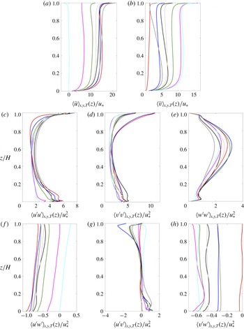
Having established that Langmuir cells with varying levels of coherence remain present under a range of realistic forcing conditions in coastal environments, it is prudent now to assess how turbulence statistics vary within the column. This analysis will provide yet more insight on how the intensity of mixing affects levels of large-scale coherence within the column. For the purpose of this article, first- and second-order turbulence statistics are sufficient, which are shown in figure 5. Figures 5(a,b) and 5(c–h) show first- and second-order statistics, respectively. Note that the stresses shown in figure 5(c–h) are the ‘total’, or Reynolds, stresses, which are recovered from LES as a post-processing exercise via addition of the resolved and subgrid-scale components,
 $\langle \boldsymbol{u}^{\prime }\otimes \boldsymbol{u}^{\prime }\rangle _{T}=\langle \tilde{\boldsymbol{u}}^{\prime }\otimes \tilde{\boldsymbol{u}}^{\prime }\rangle _{T}+\boldsymbol{\unicode[STIX]{x1D70F}}$
. Specific details of the cases are provided in the figure caption, and in table 1.
Vertical profiles of (a,b) first-order and (c–h) second-order flow quantities of different misalignment cases. Axis labels denote quantities, where stresses in (c–h) represent ‘total’, or Reynolds-averaged, which are the sum of the subgrid-scale and resolved stresses. Red:
 $\unicode[STIX]{x1D703}_{1}=0^{\circ }$
,
 $\unicode[STIX]{x1D703}_{2}=0^{\circ }$
(Case
 $C_{2211}$
); blue:
 $\unicode[STIX]{x1D703}_{1}=30^{\circ }$
,
 $\unicode[STIX]{x1D703}_{2}=0^{\circ }$
(Case
 $C_{2221}$
); green:
 $\unicode[STIX]{x1D703}_{1}=60^{\circ }$
,
 $\unicode[STIX]{x1D703}_{2}=0^{\circ }$
(Case
 $C_{2241}$
); magenta:
 $\unicode[STIX]{x1D703}_{1}=90^{\circ }$
,
 $\unicode[STIX]{x1D703}_{2}=0^{\circ }$
(Case
 $C_{2251}$
); cyan:
 $\unicode[STIX]{x1D703}_{1}=120^{\circ }$
,
 $\unicode[STIX]{x1D703}_{2}=0^{\circ }$
(Case
 $C_{2261}$
); black:
 $\unicode[STIX]{x1D703}_{1}=45^{\circ }$
,
 $\unicode[STIX]{x1D703}_{2}=45^{\circ }$
(Case
 $C_{2234}$
); dark grey:
 $\unicode[STIX]{x1D703}_{1}=30^{\circ }$
,
 $\unicode[STIX]{x1D703}_{2}=60^{\circ }$
(Case
 $C_{2225}$
); light grey:
 $\unicode[STIX]{x1D703}_{1}=45^{\circ }$
,
 $\unicode[STIX]{x1D703}_{2}=30^{\circ }$
(Case
 $C_{2233}$
). Note that the profiles shown correspond to all of Set 3 (
 $C_{22i1}$
, red, blue, green, magenta and cyan), all of Set 7 (
 $C_{223i}$
, light grey and black) and a single case from Set 6 (
 $C_{2225}$
, dark grey).

The Reynolds-averaged streamwise (figure 5
a) and spanwise (figure 5
b) velocity profiles provide major insights into the bulk transport of the column under changing conditions. In figure 5(a), the limiting maximum profile of Case
 $C_{2211}$
(red) corresponds with coaligned wind, wave and column pressure-gradient forcing, while the limiting minimum profile of Case
 $C_{2261}$
(cyan) corresponds with wind and wave forcing imposed at
 $\unicode[STIX]{x1D703}_{1}=120^{\circ }$
and
 $\unicode[STIX]{x1D703}_{2}=0$
(i.e. opposing the ambient column pressure gradient). Between these limiting profiles, the velocities vary monotonically as the role of wind and wave forcing alters the balance of streamwise momentum. For the limiting maximum profile, this case also imposes the largest hydrodynamic drag (evidenced by the bottom-boundary-layer wall-normal gradient). The profiles all exhibit a pronounced gradient at
 $z/H\approx 0.9$
: this gradient is induced by atmospheric surface layer drag, which is imposed at the sea surface level (and defined via the
 $\unicode[STIX]{x1D6F9}_{1}$
parameter). As expected, the vertical profiles for spanwise velocity are effectively a reverse (in terms of order, not magnitude) of the streamwise profiles. Although every effort was made to attain a true Reynolds average, it is apparent from figure 5(b), for Case
 $C_{2211}$
(red), that some transience is retained within the averages (for this case, since the imposed forcing is all aligned in the streamwise direction, Reynolds-averaged spanwise transport should be zero). Nevertheless, a modest value remains. As the wind and wave forcing is rotated through a range of obliquity angles, the value of
 $\langle \tilde{v}\rangle _{xyT}(z)/u_{\ast }$
increases, which occurs as a momentum balance develops in the spanwise direction. Note, too, that for the oblique cases (where the asymptotic example in figure 5
b corresponds to Case
 $C_{2261}$
), a pronounced bottom boundary layer develops, even though the pressure gradient – which would ordinarily be responsible for bottom-boundary-layer shear – is aligned in the
 $x$
direction.
Figures 5(c–e) and 5(f–h) correspond to the normal and shear components of the Reynolds stress tensor, as denoted by the abscissa labels. Beginning firstly with the streamwise-normal component of the stress tensor (figure 5
c), it is clear, firstly, that the largest bottom-boundary-layer value occurs for
 $C_{2211}$
– the case for which all forces are coaligned in the streamwise direction and for which the bottom-bed shear is greatest (figure 5
a). The bottom-boundary-layer streamwise-normal stresses decrease monotonically until Case
 $C_{2261}$
. In the upper regions, however, there is a seeming reversal in the values of
 $\langle \tilde{u} ^{\prime }\tilde{u} ^{\prime }\rangle _{xyT}/u_{\ast }^{2}$
, with the largest values being associated with Cases
 $C_{2221}$
(blue) and
 $C_{2225}$
(dark grey). Recall, however, that figure 3(k,l) provides instantaneous and two-point correlation contours for these cases, which indicated that these exhibited the lowest
 $\unicode[STIX]{x1D6FE}$
(also summarized in table 1). With this, it is clear that the largest
 $\langle \tilde{u} ^{\prime }\tilde{u} ^{\prime }\rangle _{xyT}/u_{\ast }^{2}$
values occur, in general, when the cells are aligned with the streamwise direction. Likewise, the spanwise stresses show similar patterns, where elevated mixing in the upper layer is most pronounced due to fluctuations superimposed upon the counter-rotating large-scale Langmuir cells (see profiles for Cases
 $C_{2211}$
, red; and
 $C_{2221}$
, blue).
For all cases, figure 5(e) shows elevated
 $\langle \tilde{w}^{\prime }\tilde{w}^{\prime }\rangle _{xyT}/u_{\ast }^{2}$
within the central regions of the column,
 $0.4\lesssim z/H\lesssim 0.8$
, where the streamwise- and spanwise-normal stresses were smallest. This is a product of the vertical transport associated with convergence and divergence at the surface, which directs high-
 $tke$
fluid in the vertical (figure 6, indeed, confirms that shear production of
 $tke$
is dominant at the surface and bottom-boundary-layer regions (McWilliams et al.
Reference McWilliams, Sullivan and Moeng1997; Harcourt Reference Harcourt2013; Sinha et al.
Reference Sinha, Tejada-Martínez and Akan2015; Deng et al.
Reference Deng, Yang, Xuan and Shen2019).
Figure 5(f–h) shows the Reynolds shear stress profiles,
 $\langle \tilde{u} ^{\prime }\tilde{w}^{\prime }\rangle _{xyT}/u_{\ast }^{2}$
(figure 5
f),
 $\langle \tilde{u} ^{\prime }\tilde{v}^{\prime }\rangle _{xyT}/u_{\ast }^{2}$
(figure 5
g) and
 $\langle \tilde{v}^{\prime }\tilde{w}^{\prime }\rangle _{xyT}/u_{\ast }^{2}$
(figure 5
h). Here
 $\langle \tilde{u} ^{\prime }\tilde{w}^{\prime }\rangle _{xyT}/u_{\ast }^{2}$
represents the column streamwise–wall-normal momentum fluxes, and at the domain bottom and top represents the bottom-bed shear and imposed atmospheric drag, respectively, for the case of coaligned forcing. Indeed, the Case
 $C_{2211}$
profile (red) indicates the largest bottom-bed stresses, which corresponds to linear momentum balance against the imposed pressure-gradient forcing (
 $\boldsymbol{e}_{x}\unicode[STIX]{x1D6F1}(H/u_{\ast }^{2})$
in (2.7), and accompanying text). As the forces are imposed at larger obliquity angles, we observe a monotonic decrease in the imposed bottom-bed stress.
Vertical profiles of normalized
 $tke$
shear production,
 ${\mathcal{P}}$
(a), dissipation,
 $\unicode[STIX]{x1D716}$
(b), and production by Stokes drift (c); see also (3.10) and accompanying text. The
 $tke$
terms are normalized by
 $u_{\ast }^{3}/H$
. Red:
 $\unicode[STIX]{x1D703}_{1}=0^{\circ }$
,
 $\unicode[STIX]{x1D703}_{2}=0^{\circ }$
(Case
 $C_{2211}$
); blue:
 $\unicode[STIX]{x1D703}_{1}=30^{\circ }$
,
 $\unicode[STIX]{x1D703}_{2}=0^{\circ }$
(Case
 $C_{2221}$
); green:
 $\unicode[STIX]{x1D703}_{1}=60^{\circ }$
,
 $\unicode[STIX]{x1D703}_{2}=0^{\circ }$
(Case
 $C_{2241}$
); magenta:
 $\unicode[STIX]{x1D703}_{1}=90^{\circ }$
,
 $\unicode[STIX]{x1D703}_{2}=0^{\circ }$
(Case
 $C_{2251}$
); cyan:
 $\unicode[STIX]{x1D703}_{1}=120^{\circ }$
,
 $\unicode[STIX]{x1D703}_{2}=0^{\circ }$
(Case
 $C_{2261}$
); black:
 $\unicode[STIX]{x1D703}_{1}=45^{\circ }$
,
 $\unicode[STIX]{x1D703}_{2}=45^{\circ }$
(Case
 $C_{2234}$
); dark grey:
 $\unicode[STIX]{x1D703}_{1}=30^{\circ }$
,
 $\unicode[STIX]{x1D703}_{2}=60^{\circ }$
(Case
 $C_{2225}$
); light grey:
 $\unicode[STIX]{x1D703}_{1}=45^{\circ }$
,
 $\unicode[STIX]{x1D703}_{2}=30^{\circ }$
(Case
 $C_{2233}$
). Note that the profiles shown correspond to all of Set 3 (
 $C_{22i1}$
, red, blue, green, magenta and cyan), all of Set 7 (
 $C_{223i}$
, light grey and black) and a single case from Set 6 (
 $C_{2225}$
, dark grey).

Figure 6 shows vertical profiles of constituent right-hand-side terms in the Reynolds-averaged
 $tke$
transport equation:
 $$\begin{eqnarray}\displaystyle \tilde{\boldsymbol{u}}\boldsymbol{\cdot }\unicode[STIX]{x1D735}\langle tke\rangle _{T}=\underbrace{{\mathcal{T}}}_{\mathit{Transport}}-\underbrace{\langle \boldsymbol{u}^{\prime }\otimes \boldsymbol{u}^{\prime }\rangle _{T}\boldsymbol{ : }\unicode[STIX]{x1D735}\langle \tilde{\boldsymbol{u}}\rangle _{T}}_{\mathit{Production},\,{\mathcal{P}}}-\underbrace{\langle \unicode[STIX]{x1D749}\rangle _{T}\boldsymbol{ : }\langle \unicode[STIX]{x1D64E}\rangle _{T}}_{\mathit{Dissipation},\,\unicode[STIX]{x1D716}}+\underbrace{{\displaystyle \frac{\unicode[STIX]{x1D6F9}_{2}}{\unicode[STIX]{x1D6F9}_{1}}}\;\unicode[STIX]{x1D753}_{s}\times \langle \tilde{\unicode[STIX]{x1D74E}}^{\prime }\otimes \tilde{\boldsymbol{u}}^{\prime }\rangle _{T}}_{\mathit{CL\,vortex\,forcing}},\quad & & \displaystyle\end{eqnarray}$$
where all quantities have been normalized by
 $u_{\ast }^{3}/H$
. Other researchers have used this equation to establish the contribution to
 $tke$
in different conditions (e.g. Harcourt Reference Harcourt2013; Sinha et al.
Reference Sinha, Tejada-Martínez and Akan2015; Deng et al.
Reference Deng, Yang, Xuan and Shen2019). Figure 6(a) plots production of
 $tke$
by mechanical shear, which indicates – as expected – that shear production is most pronounced in the lower and upper regions. This is a product of bottom-boundary-layer shear and Stokes shear. For all cases, the upper regions (
 $0.6\lesssim z/H\lesssim 0.9$
) indicate the potential for negative production, which is a product of the negative vertical gradient in streamwise velocity due to the Langmuir cells (i.e. figure 5
a,f; observed also by Kukulka et al. (Reference Kukulka, Pleuddemann and Sullivan2012)). Suzuki & Fox-Kemper (Reference Suzuki and Fox-Kemper2016) have developed a ‘momentum sorting’ mechanism to explain the
 $tke$
production in this region of the column, although attribution of the present results to this mechanism is beyond the scope of the present work. Since
 $tke$
is a scalar, there is no directional dependence, which simplifies comparison between cases. It is known that
 $tke$
production due to Stokes drift shear decreases with increasing misalignment (Van Roekel et al.
Reference Van Roekel, Fox-Kemper, Sullivan, Hamlington and Haney2012). Figure 6(b) plots
 $tke$
dissipation, where the profiles are similar to those reported by others for coastal-zone Langmuir turbulence (Kukulka et al.
Reference Kukulka, Pleuddemann and Sullivan2012; Tejada-Martínez et al.
Reference Tejada-Martínez, Grosch, Sinha, Akan and Martinat2012). Finally, figure 6(c) shows contributions to
 $tke$
due to the vortex forcing (‘CL vortex forcing’ in (3.10)). For the very high
 $Re_{\unicode[STIX]{x1D70F}}$
values considered for this article, the transport term contribution is negligible with the exception of locations closest to the bed and surface that are not resolved during LES (Kim, Moin & Moser Reference Kim, Moin and Moser1987). Note that the figure panels have been slightly truncated in the vertical direction at the top and bottom. The values for production and dissipation are extremely large in the bottom boundary layer and upper regions of the Stokes layer, while Stokes drift production is largest near the top of the domain. The figures show that these quantities also do not vary significantly in the interior with respect to misalignment. The figures are consistent with observations from figure 2, where we showed that the large-scale cells were least correlated in the upper and lower regions, due to strong shear and vigorous mixing.
4 Vorticity transport equation
In order to finalize the results presented in this article, we present the following development based upon streamwise vorticity transport aligned in the
 $x^{\prime \prime }$
local axis denoted in figure 1(a). We begin, first, with the transport equation for phase-averaged vorticity, which is obtained via the curl of (2.7). Phase averaging eliminates transient effects, but preserves the counter-rotating Langmuir cells, which vanish as the averaging period approaches infinity. The curl operation yields
 $$\begin{eqnarray}\displaystyle \frac{\unicode[STIX]{x2202}\tilde{\unicode[STIX]{x1D74E}}}{\unicode[STIX]{x2202}t}+\tilde{\boldsymbol{u}}\boldsymbol{\cdot }\unicode[STIX]{x1D735}\tilde{\unicode[STIX]{x1D74E}}=\tilde{\unicode[STIX]{x1D74E}}\boldsymbol{\cdot }\unicode[STIX]{x1D735}\tilde{\boldsymbol{u}}-\unicode[STIX]{x1D735}\times (\unicode[STIX]{x1D735}\boldsymbol{\cdot }\unicode[STIX]{x1D64F})+\frac{\unicode[STIX]{x1D6F9}_{2}}{\unicode[STIX]{x1D6F9}_{1}}\unicode[STIX]{x1D735}\times \boldsymbol{f}^{\unicode[STIX]{x1D714}}, & & \displaystyle\end{eqnarray}$$
where the pressure correction term and pressure-gradient forcing vanish following application of the curl operation. Here, we are interested in the component of vorticity aligned with the
 $x^{\prime \prime }$
direction (figure 1), which by definition exceeds all other vorticity components since it is aligned with the resultant Langmuir cells. Thus, we consider the relevant component of (4.1):
 $$\begin{eqnarray}\displaystyle \frac{\unicode[STIX]{x2202}\tilde{\unicode[STIX]{x1D714}}_{x^{\prime \prime }}}{\unicode[STIX]{x2202}t}+\tilde{\boldsymbol{u}}\boldsymbol{\cdot }\tilde{\unicode[STIX]{x1D714}}_{x^{\prime \prime }}=\tilde{\unicode[STIX]{x1D74E}}\boldsymbol{\cdot }\unicode[STIX]{x1D735}\tilde{u} -\unicode[STIX]{x1D716}_{1jk}\unicode[STIX]{x2202}_{j}\unicode[STIX]{x2202}_{p}\unicode[STIX]{x1D61B}_{kp}+\frac{\unicode[STIX]{x1D6F9}_{2}}{\unicode[STIX]{x1D6F9}_{1}}\unicode[STIX]{x1D716}_{1jk}\unicode[STIX]{x2202}_{j}\,f_{k}^{\unicode[STIX]{x1D714}}, & & \displaystyle\end{eqnarray}$$
where
 $\unicode[STIX]{x1D716}_{ijk}$
is the alternating unit tensor. Owing to homogeneity in the
 $x^{\prime \prime }$
direction, all partial derivatives in this direction can be eliminated from (4.2). This results in omission of the first term on the right-hand side – the stretching and tilting term,
 $\tilde{\unicode[STIX]{x1D74E}}\boldsymbol{\cdot }\unicode[STIX]{x1D735}\tilde{u} =\tilde{\unicode[STIX]{x1D714}}_{x}\unicode[STIX]{x2202}_{x}\tilde{u} +\tilde{\unicode[STIX]{x1D714}}_{y}\unicode[STIX]{x2202}_{y}\tilde{u} +\tilde{\unicode[STIX]{x1D714}}_{z}\unicode[STIX]{x2202}_{z}\tilde{u}$
– where the first term automatically vanishes, while the second and third terms cancel one another following substitution of
 $\tilde{\unicode[STIX]{x1D714}}_{y}$
and
 $\tilde{\unicode[STIX]{x1D714}}_{z}$
and expansion. The second term on the right-hand side, hereafter called turbulent torque, can be simplified upon introduction of Boussinesq model,
 $\unicode[STIX]{x1D64F}=-2\unicode[STIX]{x1D708}_{t}(\unicode[STIX]{x1D64E})+(2/3)\unicode[STIX]{x1D739}tke$
, where
 $\unicode[STIX]{x1D708}_{t}$
is a turbulent viscosity,
 $\unicode[STIX]{x1D64E}$
is the strain-rate tensor,
 $\unicode[STIX]{x1D739}$
is the Kronecker delta and
 $tke$
is turbulent kinetic energy (Pope Reference Pope2000). In the following development,
 $\unicode[STIX]{x1D708}_{t}$
is presumed to exhibit weak spatial heterogeneity as a matter of convenience. The purpose of this section is mathematical explanation of the observed attenuation in Langmuir cell intensity with diverging imposed forces: generalization for spatial heterogeneity in
 $\unicode[STIX]{x1D708}_{t}$
is not expected to substantially influence the deductions reported below. Following a series of algebraic developments, it can be shown that the Laplacian of vorticity emerges:
 $$\begin{eqnarray}\displaystyle -\unicode[STIX]{x1D735}\times (\unicode[STIX]{x1D735}\boldsymbol{\cdot }\unicode[STIX]{x1D64F})=-{\textstyle \frac{1}{2}}\unicode[STIX]{x1D708}_{t}(\unicode[STIX]{x2202}_{z}^{2}\tilde{\unicode[STIX]{x1D714}}_{x^{\prime \prime }}+\unicode[STIX]{x2202}_{y^{\prime \prime }}^{2}\tilde{\unicode[STIX]{x1D714}}_{x^{\prime \prime }}). & & \displaystyle\end{eqnarray}$$
The last term on the right-hand side is the curl of the vortex forcing term, which is responsible for sustenance of the Langmuir circulations, and needs more attention. We have seen that a new
 $\{x^{\prime \prime },y^{\prime \prime },z\}$
coordinate system has been assigned, from which it follows that the Stokes drift is aligned at an angle,
 $\unicode[STIX]{x1D703}_{1}+\unicode[STIX]{x1D703}_{2}-\unicode[STIX]{x1D6FE}$
, from the
 $x^{\prime \prime }$
direction (figure 1). Here, let us define that
 $\unicode[STIX]{x1D6FE}^{\ast }=\unicode[STIX]{x1D703}_{1}+\unicode[STIX]{x1D703}_{2}-\unicode[STIX]{x1D6FE}$
. Hence, in the
 $\{x^{\prime \prime },y^{\prime \prime },z\}$
coordinate system, equation (2.13) becomes
 $$\begin{eqnarray}\displaystyle \boldsymbol{f}^{\unicode[STIX]{x1D714}} & = & \displaystyle \unicode[STIX]{x1D719}_{s}(z,k)\sin (\unicode[STIX]{x1D6FE}^{\ast })(\unicode[STIX]{x2202}_{x^{\prime \prime }}\tilde{v}-\unicode[STIX]{x2202}_{y^{\prime \prime }}\tilde{u} )\hat{i} -\unicode[STIX]{x1D719}_{s}(z,k)\cos (\unicode[STIX]{x1D6FE}^{\ast })(\unicode[STIX]{x2202}_{x^{\prime \prime }}\tilde{v}-\unicode[STIX]{x2202}_{y^{\prime \prime }}\tilde{u} ){\hat{j}}\nonumber\\ \displaystyle & & \displaystyle +\,\unicode[STIX]{x1D719}_{s}(z,k)[\cos (\unicode[STIX]{x1D6FE}^{\ast })(\unicode[STIX]{x2202}_{z}\tilde{u} -\unicode[STIX]{x2202}_{x^{\prime \prime }}\tilde{w})-\sin (\unicode[STIX]{x1D6FE}^{\ast })(\unicode[STIX]{x2202}_{y^{\prime \prime }}\tilde{w}-\unicode[STIX]{x2202}_{z}\tilde{v})]\hat{k}.\end{eqnarray}$$
Then, taking the curl of
 $\boldsymbol{f}^{\unicode[STIX]{x1D714}}$
and further simplifying, we recover the
 $\hat{i}$
component, as
 $$\begin{eqnarray}\displaystyle \unicode[STIX]{x1D735}\times \boldsymbol{f}^{\unicode[STIX]{x1D714}}=-\left(\frac{\unicode[STIX]{x2202}\tilde{u} }{\unicode[STIX]{x2202}y^{\prime \prime }}\frac{\text{d}}{\text{d}z}(\unicode[STIX]{x1D719}_{s}(z,k)\cos (\unicode[STIX]{x1D6FE}^{\ast }))+\unicode[STIX]{x1D719}_{s}(z,k)\sin (\unicode[STIX]{x1D6FE}^{\ast })\frac{\unicode[STIX]{x2202}\tilde{\unicode[STIX]{x1D714}}_{x^{\prime \prime }}}{\unicode[STIX]{x2202}y^{\prime \prime }}\right)\hat{i} . & & \displaystyle\end{eqnarray}$$
Based on preceding developments, equation (4.2) reduces to
 $$\begin{eqnarray}\displaystyle \tilde{v}\frac{\unicode[STIX]{x2202}\tilde{\unicode[STIX]{x1D714}}_{x^{\prime \prime }}}{\unicode[STIX]{x2202}y^{\prime \prime }}+\tilde{w}\frac{\unicode[STIX]{x2202}\tilde{\unicode[STIX]{x1D714}}_{x^{\prime \prime }}}{\unicode[STIX]{x2202}z} & = & \displaystyle -\frac{1}{2}\unicode[STIX]{x1D708}_{t}\left(\frac{\unicode[STIX]{x2202}^{2}}{\unicode[STIX]{x2202}z^{2}}\tilde{\unicode[STIX]{x1D714}}_{x^{\prime \prime }}+\frac{\unicode[STIX]{x2202}^{2}}{\unicode[STIX]{x2202}{y^{\prime \prime }}^{2}}\tilde{\unicode[STIX]{x1D714}}_{x^{\prime \prime }}\right)\nonumber\\ \displaystyle & & \displaystyle -\,\frac{\unicode[STIX]{x1D6F9}_{2}}{\unicode[STIX]{x1D6F9}_{1}}\left(\frac{\unicode[STIX]{x2202}\tilde{u} }{\unicode[STIX]{x2202}y^{\prime \prime }}\frac{\text{d}}{\text{d}z}(\unicode[STIX]{x1D719}_{s}(z,k)\cos (\unicode[STIX]{x1D6FE}^{\ast }))+\unicode[STIX]{x1D719}_{s}(z,k)\sin (\unicode[STIX]{x1D6FE}^{\ast })\left(\frac{\unicode[STIX]{x2202}}{\unicode[STIX]{x2202}y^{\prime \prime }}\tilde{\unicode[STIX]{x1D714}}_{x^{\prime \prime }}\right)\right).\nonumber\\ \displaystyle & & \displaystyle\end{eqnarray}$$
In its present form, further deductions from (4.6) are not possible, owing to the presence of spanwise and vertical gradients. This, however, does not preclude local consideration of (4.6), where careful selection does enable further simplifications. One such location is a vertical profile placed at the centre of a Langmuir cell, where
 $\tilde{w}=0$
and
 $\unicode[STIX]{x2202}_{y^{\prime \prime }}\tilde{\unicode[STIX]{x1D714}}_{x^{\prime \prime }}=0$
. One such transect, A–A, is shown on the idealized schematic of figure 7. Moreover, the system reductions can be appreciated from introduction of a leading-order model for the Langmuir cells in the form of a streamfunction:
 $$\begin{eqnarray}\displaystyle \unicode[STIX]{x1D713}(y^{\prime \prime },z)=\unicode[STIX]{x1D712}\sin (k_{y^{\prime \prime }}\unicode[STIX]{x03C0}y^{\prime \prime })\sin (k_{z}\unicode[STIX]{x03C0}z), & & \displaystyle\end{eqnarray}$$
where
 $k_{y^{\prime \prime }}=2/H$
,
 $k_{z}=1/H$
and
 $\unicode[STIX]{x1D712}$
is an amplitude. With the streamfunction, we can recover all flow components in the
 $y^{\prime \prime }{-}z$
plane:
 $$\begin{eqnarray}\displaystyle & \displaystyle \tilde{\unicode[STIX]{x1D714}}_{x^{\prime \prime }}(y^{\prime \prime },z)=-\unicode[STIX]{x1D6FB}^{2}\unicode[STIX]{x1D713}=\unicode[STIX]{x1D712}(k_{y}^{2}+k_{z}^{2})\unicode[STIX]{x03C0}^{2}\sin (k_{y^{\prime \prime }}\unicode[STIX]{x03C0}y^{\prime \prime })\sin (k_{z}\unicode[STIX]{x03C0}z), & \displaystyle\end{eqnarray}$$
 $$\begin{eqnarray}\displaystyle & \displaystyle \tilde{v}(y^{\prime \prime },z)=\unicode[STIX]{x2202}_{z}\unicode[STIX]{x1D713}=\unicode[STIX]{x1D712}k_{z}\unicode[STIX]{x03C0}\sin (k_{y^{\prime \prime }}\unicode[STIX]{x03C0}y^{\prime \prime })\cos (k_{z}\unicode[STIX]{x03C0}z) & \displaystyle\end{eqnarray}$$
and
 $$\begin{eqnarray}\displaystyle & \displaystyle \tilde{w}(y^{\prime \prime },z)=-\unicode[STIX]{x2202}_{y^{\prime \prime }}\unicode[STIX]{x1D713}=-\unicode[STIX]{x1D712}k_{y^{\prime \prime }}\unicode[STIX]{x03C0}\cos (k_{y^{\prime \prime }}\unicode[STIX]{x03C0}y^{\prime \prime })\sin (k_{z}\unicode[STIX]{x03C0}z), & \displaystyle\end{eqnarray}$$
with (4.8), (4.9) and (4.10), it is evident that at
 $y^{\prime \prime }=L/4$
,
 $\unicode[STIX]{x2202}_{y^{\prime \prime }}\tilde{\unicode[STIX]{x1D714}}_{x^{\prime \prime }}=\tilde{w}=0$
by virtue of the cosine function in (4.8) and (4.10).
Schematic of idealized (leading-order projection) Langmuir cells in the
 $y^{\prime \prime }{-}z$
plane. Transect A–A used in § 4 development is shown, for perspective.

Applying these conditions, and only at the centre of the Langmuir cell, equation (4.6) reduces to
 $$\begin{eqnarray}\displaystyle \frac{1}{2}\unicode[STIX]{x1D708}_{t}{\displaystyle \frac{\text{d}^{2}\tilde{\unicode[STIX]{x1D714}}_{x^{\prime \prime }}}{\text{d}z^{2}}}=-\frac{\unicode[STIX]{x1D6F9}_{2}}{\unicode[STIX]{x1D6F9}_{1}}{\displaystyle \frac{\text{d}}{\text{d}z}}(\unicode[STIX]{x1D719}_{s}(z,k)\cos (\unicode[STIX]{x1D6FE}^{\ast })){\displaystyle \frac{\unicode[STIX]{x2202}\tilde{u} }{\unicode[STIX]{x2202}y^{\prime \prime }}}. & & \displaystyle\end{eqnarray}$$
Integration of (4.11) with respect to
 $z$
yields
 $$\begin{eqnarray}\displaystyle \frac{1}{2}\unicode[STIX]{x1D708}_{t}{\displaystyle \frac{\text{d}\tilde{\unicode[STIX]{x1D714}}_{x^{\prime \prime }}}{\text{d}z}}=-\frac{\unicode[STIX]{x1D6F9}_{2}}{\unicode[STIX]{x1D6F9}_{1}}\;\unicode[STIX]{x1D719}_{s}(z,k)\cos (\unicode[STIX]{x1D6FE}^{\ast }){\displaystyle \frac{\unicode[STIX]{x2202}\tilde{u} }{\unicode[STIX]{x2202}y^{\prime \prime }}}. & & \displaystyle\end{eqnarray}$$
Upon further integration with respect to
 $z$
, and following a series of modest algebraic developments, we recover
 $$\begin{eqnarray}\displaystyle \tilde{\unicode[STIX]{x1D714}}_{x^{\prime \prime }}=-\frac{2}{\unicode[STIX]{x1D708}_{t}}\;\frac{\unicode[STIX]{x1D6F9}_{2}}{\unicode[STIX]{x1D6F9}_{1}}\;\cos (\unicode[STIX]{x1D6FE}^{\ast }){\displaystyle \frac{\unicode[STIX]{x2202}\tilde{u} }{\unicode[STIX]{x2202}y^{\prime \prime }}}\int _{0}^{H}\left[\frac{\cosh [2kz]}{2\sinh ^{2}[kH]}\right]\text{d}z. & & \displaystyle\end{eqnarray}$$
In the above equation, the integrand,
 $\unicode[STIX]{x1D719}_{s}(z,k)$
, is only a function of
 $k$
(wavenumber) and
 $z$
, where
 $k$
can be assumed from physically motivated wave parameters as in § 2.3, and can be integrated with respect to
 $z$
. However, in the present context where we seek to understand the influence of
 $\unicode[STIX]{x1D6FE}^{\ast }$
on the vorticity dynamics, we can simplify the development through introduction of the parameter
 $\unicode[STIX]{x1D701}(z)=-2/\unicode[STIX]{x1D708}_{t}(\unicode[STIX]{x2202}_{y^{\prime \prime }}\tilde{u} )\int _{0}^{H}\unicode[STIX]{x1D719}_{s}(z,k)\text{d}z$
, which yields
 $$\begin{eqnarray}\displaystyle \tilde{\unicode[STIX]{x1D714}}_{x^{\prime \prime }}=\unicode[STIX]{x1D701}(z)\cos (\unicode[STIX]{x1D6FE}^{\ast })\frac{\unicode[STIX]{x1D6F9}_{2}}{\unicode[STIX]{x1D6F9}_{1}}. & & \displaystyle\end{eqnarray}$$
Equation (4.14) explains that the magnitude of
 $\tilde{\unicode[STIX]{x1D714}}_{x^{\prime \prime }}$
is maximum when
 $\unicode[STIX]{x1D6FE}^{\ast }$
is
 $0$
, i.e. when the wind, wave and mean current directions are coaligned, and diminishes as
 $\unicode[STIX]{x1D6FE}^{\ast }$
deviates from
 $0$
, as seen in figure 8. Moreover, the equation also confirms a linear dependence upon
 $\unicode[STIX]{x1D6F9}_{2}$
, and a dependence on wind stress as
 ${\sim}\unicode[STIX]{x1D6F9}_{1}^{-1}$
. In order to place this development in a context relevant to the figure 4 results, which always showed that
 $\unicode[STIX]{x1D6FE}<(\unicode[STIX]{x1D703}_{1}+\unicode[STIX]{x1D703}_{2})$
, equation (4.14) can be advanced further:
 $$\begin{eqnarray}\displaystyle \unicode[STIX]{x1D6FE}^{\ast }=\arccos \left({\displaystyle \frac{\tilde{\unicode[STIX]{x1D714}}_{x^{\prime \prime }}}{\unicode[STIX]{x1D701}(z)}}{\displaystyle \frac{\unicode[STIX]{x1D6F9}_{1}}{\unicode[STIX]{x1D6F9}_{2}}}\right)=\unicode[STIX]{x1D703}_{1}+\unicode[STIX]{x1D703}_{2}-\unicode[STIX]{x1D6FE}, & & \displaystyle\end{eqnarray}$$
from which it can be shown that
 $$\begin{eqnarray}\displaystyle {\displaystyle \frac{\unicode[STIX]{x1D6FE}}{\unicode[STIX]{x1D703}_{1}+\unicode[STIX]{x1D703}_{2}}}=1-{\displaystyle \frac{\arccos \left({\displaystyle \frac{\tilde{\unicode[STIX]{x1D714}}_{x^{\prime \prime }}}{\unicode[STIX]{x1D701}(z)}}{\displaystyle \frac{\unicode[STIX]{x1D6F9}_{1}}{\unicode[STIX]{x1D6F9}_{2}}}\right)}{\unicode[STIX]{x1D703}_{1}+\unicode[STIX]{x1D703}_{2}}}. & & \displaystyle\end{eqnarray}$$
This development constitutes a theoretical justification for the prior results on the relationship between
 $\unicode[STIX]{x1D6FE}$
and angles
 $\unicode[STIX]{x1D703}_{1}$
and
 $\unicode[STIX]{x1D703}_{2}$
, and specifically addresses the question of why
 $\unicode[STIX]{x1D6FE}<(\unicode[STIX]{x1D703}_{1}+\unicode[STIX]{x1D703}_{2})$
. Figure 8 presents profiles for the normalized vorticity with respect to
 $\unicode[STIX]{x1D6FE}^{\ast }$
, and for increasing
 $\unicode[STIX]{x1D6F9}_{2}$
. The profiles are precisely as expected – the strongest values occur for coalignment, and systematic misalignment monotonically decreases the resultant streamwise vorticity (again, where ‘streamwise’ denotes the
 $x^{\prime \prime }$
direction). It would be desirable to perform quantitative comparison of the predictions from LES with the model results. However, such point-to-point comparison is not possible due to the need to define unknown parameters a priori (
 $\unicode[STIX]{x1D708}_{t}$
,
 $\tilde{\unicode[STIX]{x1D714}}_{x^{\prime \prime }}$
and quantities defining
 $\unicode[STIX]{x1D701}(z)$
). We stress, however, that the present derivation was not intended to yield predictions for
 $\unicode[STIX]{x1D6FE}$
; rather, we were seeking to establish a basis for the results in § 3.1, wherein
 $\unicode[STIX]{x1D6FE}$
was always intermediate to the imposed forces. To this extent, the derivation is useful, but its prognostic utility is limited – the existing model from Van Roekel et al. (Reference Van Roekel, Fox-Kemper, Sullivan, Hamlington and Haney2012) (equation (3.3)) is ideally suited for such purposes for open-ocean conditions, or the version generalized for coastal conditions presented here (3.4).
Plot of
 $\tilde{\unicode[STIX]{x1D714}}_{x^{\prime \prime }}/\unicode[STIX]{x1D701}(z)$
versus
 $\unicode[STIX]{x1D6FE}^{\ast }$
. The figure illustrates the diminishing strength of Langmuir cells with increasing misalignment between the wind, wave and mean current forcing. The profiles correspond to
 $\unicode[STIX]{x1D6F9}_{2}/\unicode[STIX]{x1D6F9}_{1}=10$
(inner profile), 15, 20, 25 and 30 (outer profile) in (4.14), where the values of
 $\unicode[STIX]{x1D6F9}_{2}/\unicode[STIX]{x1D6F9}_{1}$
are based on table 1 cases.

5 Conclusion
We investigated the influence of misaligned mean current, interacting with wind and wave, on the orientation and structure of coastal Langmuir cells. There has been prior work on the spatial and dynamical nature of Langmuir turbulence in coastal environments (Gargett et al.
Reference Gargett, Wells, Tejada-Martínez and Grosch2004; Gargett & Wells Reference Gargett and Wells2007; Tejada-Martínez & Grosch Reference Tejada-Martínez and Grosch2007; Martinat et al.
Reference Martinat, Xu, Grosch and Tejada-Martínez2011; Li et al.
Reference Li, Li, Gerbi and Song2013; Shrestha et al.
Reference Shrestha, Anderson and Kuehl2018; Deng et al.
Reference Deng, Yang, Xuan and Shen2019), but the overwhelming majority of such work has focused on the case of coaligned wind, wave and current forcing – an arrangement expected to be the exception, not the norm, in realistic settings. In this article, we have used LES to study the nature of Langmuir turbulence under a range of variable forcing conditions – forcing magnitude and obliquity – and the results have been used to characterize the aggregate response of resultant cells. Foremost among the results presented herein is evidence that the oblique forcing, nevertheless, yields coherent cells aligned at an angle intermediate to the range of imposed forces. The coherence diminishes, but never vanishes entirely, for extreme obliquity angles. We found that the cell coherence was strongest throughout the intermediate depths of the column, and this was further explained by the presentation of vertical profiles of the Reynolds stress components and constituent terms in the
 $tke$
transport equation.
Results for the aggregate cell alignment,
 $\unicode[STIX]{x1D6FE}$
, were always intermediate to the wind/wave forcing and the pressure-gradient forcing. This result was further explained via presentation of a prognostic model for cell inclination, inspired by an earlier model from Van Roekel et al. (Reference Van Roekel, Fox-Kemper, Sullivan, Hamlington and Haney2012). As a final effort, we performed an assessment of the terms affecting sustenance of streamwise vorticity about a local axis aligned with the cells,
 $x^{\prime \prime }$
. The theoretical development offered further support for the simulation results. In all the cases considered,
 $\unicode[STIX]{x1D703}_{2}>0$
, such that
 $\unicode[STIX]{x1D703}_{1}+\unicode[STIX]{x1D703}_{2}>0$
. As an additional effort, we could have considered cases with
 $\unicode[STIX]{x1D703}_{2}<0$
– such that the Stokes drift is imposed at an angle between the wind and pressure-gradient directions. However, the results presented in figure 4(c) showed that the dependence on
 $\unicode[STIX]{x1D703}_{2}$
was almost negligible, relative to
 $\unicode[STIX]{x1D703}_{1}$
, while assessment of the vorticity transport equation (§ 4) shows that
 $\unicode[STIX]{x1D6FE}$
will always be intermediate to the imposed forces.
Acknowledgements
This research was supported by the Texas General Land Office, Oil Spill Program (Program Manager: S. Buschang) under TGLO contract nos 16-019-0009283 and 18-130-000-A670. Computational resources were provided by Texas Advanced Computing Center at the University of Texas at Austin.