


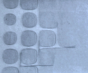



1. Introduction
In a reactive medium, the transformation from a fresh state to a fully reacted state might occur homogeneously, i.e. at the same rate at all places. However, due to local initiations in the bulk or at boundaries, it actually takes place inhomogeneously, i.e. with a progress variable depending on space and time. Then, the competition between diffusion and reaction causes the change of the medium to occur by the propagation of a front which separates the fresh and fully reacted phases and displays a definite thickness and a definite velocity (Fischer Reference Fischer1937; Kolmogorov, Petrovskii & Piskunov Reference Kolmogorov, Petrovskii and Piskunov1937; Field & Burger Reference Field and Burger1985; Williams Reference Williams1985; Goriely Reference Goriely1995; van Saarloos Reference van Saarloos2003).
In many situations of practical interest, the reactive medium is a fluid that is usually stirred by flows for intrinsic (buoyancy, instability) or extrinsic (moving boundaries, rotational force field) reasons. This is the case in chemical engineering (Ottino Reference Ottino1994) or in combustion (Williams Reference Williams1985) but also in epidemics (Russell et al. Reference Russell, Smith, Waller, Childs and Real2004), chemohydrodynamics (De Wit Reference De Wit2020; Mukherjee & Paul Reference Mukherjee and Paul2022), environment (Edouard et al. Reference Edouard, Legras, Lefèvre and Eymard1996) or ecology (Abraham Reference Abraham1998; Abraham et al. Reference Abraham, Law, Boyd, Lavender, Maldonado and Bowie2000). Then, an additional transport phenomenon, advection, competes with diffusion and reaction. Depending on the scale of the vortices, it can simply transport the reacting medium at distant locations or, more intrusively, mix the reactive species within the front thickness.
An interesting situation to highlight the implication of advection on front propagation relates to steady closed flows (Audoly, Berestycki & Pomeau Reference Audoly, Berestycki and Pomeau2000; Abel et al. Reference Abel, Celani, Vergni and Vulpiani2001, Reference Abel, Cencini, Vergni and Vulpiani2002; Cencini et al. Reference Cencini, Torcini, Vergni and Vulpiani2003; Vladimirova et al. Reference Vladimirova, Constantin, Kiselev, Ruchayskiy and Ryzhik2003; Paoletti & Solomon Reference Paoletti and Solomon2005; Pocheau & Harambat Reference Pocheau and Harambat2006, Reference Pocheau and Harambat2008; Mahoney et al. Reference Mahoney, Bargteil, Kingsbury, Mitchell and Solomon2012; Tzella & Vanneste Reference Tzella and Vanneste2014, Reference Tzella and Vanneste2015, Reference Tzella and Vanneste2019; Beauvier, Bodea & Pocheau Reference Beauvier, Bodea and Pocheau2016, Reference Beauvier, Bodea and Pocheau2017). Then, as streamlines are confined to compact regions, no large-scale advection of the medium and thus no net kinematic effect are expected at long times on fluid particles. However, due to the ability of fronts to cross streamlines, there nevertheless appears a net effect of advection on front propagation through a global enhancement of the mean front velocity and, ultimately, of the reacting rate of the stirred media (Williams Reference Williams1985; Audoly et al. Reference Audoly, Berestycki and Pomeau2000; Abel et al. Reference Abel, Celani, Vergni and Vulpiani2001, Reference Abel, Cencini, Vergni and Vulpiani2002; Cencini et al. Reference Cencini, Torcini, Vergni and Vulpiani2003; Vladimirova et al. Reference Vladimirova, Constantin, Kiselev, Ruchayskiy and Ryzhik2003; Paoletti & Solomon Reference Paoletti and Solomon2005; Pocheau & Harambat Reference Pocheau and Harambat2006, Reference Pocheau and Harambat2008; Mahoney et al. Reference Mahoney, Bargteil, Kingsbury, Mitchell and Solomon2012; Tzella & Vanneste Reference Tzella and Vanneste2014, Reference Tzella and Vanneste2015, Reference Tzella and Vanneste2019; Beauvier et al. Reference Beauvier, Bodea and Pocheau2016, Reference Beauvier, Bodea and Pocheau2017). Depending on the system, this can be beneficial (reduced time in chemical industry, increased power of internal combustion engines) or detrimental (increased spread of epidemic, growth of the ozone hole). In both cases, progress in our understanding of the behaviour of a propagating front in stirred media will be of great help in promoting or controlling this phenomenon.
Of course, the velocity enhancement of a reaction–diffusion (RD) front by stirring flows is directly related to the vortex amplitude  $U$. However, certain spatial scales of the system, vortex scales, front thickness and container dimensions, may also play a role. This study aims at examining experimentally whether, and to what extent, these spatial scales actually influence the mean velocity of a RD front propagating in a stirred medium. In addition to an improved understanding of the advection–reaction–diffusion (ARD) mechanisms, this should help to discriminate regimes where spatial scales have to be taken into account from those where they can be overlooked.
Our experiment addresses the propagation of a RD front in a Hele-Shaw cell stirred by a vortex lattice induced by magnetohydrodynamic forcing. Since the reaction is athermal, no additional convective flow is generated. Vortices have the same width  $L$ and a depth
 $d$ that is fixed by that of the cell. They provide closed steady cellular flows involving no mean flow. As they extend over a lattice comprising several lines, all of them undergo stress-free boundary conditions (b.c.), except those adjacent to the sidewalls. In addition to the front thickness
 $\lambda$, the vortex scales
 $L$ and
 $d$ provide the relevant spatial scales of this ARD system. The proper front velocity, i.e. the propagation velocity of a planar front in a fluid at rest, will be denoted
 $V_0$ and will be used to non-dimensionalize vortex amplitude and mean front velocity.
Here, we seek to experimentally determine the role of these spatial scales on the propagation of fronts, in particular on their mean propagation velocity  $V$ over the stirred medium. A previous study concluded to the independence of the mean reduced velocity
 $V/V_0$ on the aspect ratio
 $L/d$ of vortices (Beauvier et al. Reference Beauvier, Bodea and Pocheau2016, Reference Beauvier, Bodea and Pocheau2017). Following it, we will focus attention on the dependence of
 $V/V_0$ on the vortex to front scale ratio
 $L/\lambda$.
We find a scale-invariant regime at small  $U/V_0$ and a scale-dependent one at large
 $U/V_0$, and we characterize the transition between them. We then determine the relationships between
 $V/V_0$,
 $U/V_0$ and
 $L/\lambda$ in both regimes and compare with numerical simulations (Vladimirova et al. Reference Vladimirova, Constantin, Kiselev, Ruchayskiy and Ryzhik2003) and theoretical analysis (Tzella & Vanneste Reference Tzella and Vanneste2014, Reference Tzella and Vanneste2015, Reference Tzella and Vanneste2019) of ARD dynamics in a plane. Altogether, our study thus improves the characterization of front propagation in stirred flows and provides a detailed identification of a scale-invariant regime where spatial scales may be overlooked and of a scale-dependent regime where they significantly influence front propagation.
The paper is organized as follows. We first review in § 2 the main variables and regimes involved in ARD systems, with emphasis on the scale dependence of the mean front velocity. In particular, we recall previous experimental results on the independence towards the vortex aspect ratio  $L/d$ and report the various regimes found in numerical simulations and theoretical analysis. We then describe in § 3 the experimental set-up and how its available ranges of variables match with the expected regimes. The experimental results are reported and analysed in § 4. They are followed in § 5 by a discussion of the regimes encountered and their transition. A general conclusion ends the study.
2. Front propagation in cellular flows: variables and regimes
We consider a reacting medium stirred by steady cellular vortex flows involving no mean flow. We track the evolution of the reaction by a single progress variable  $\theta$,
 $0\leq \theta \leq 1$, where
 $\theta =0$ denotes the fresh state where reaction has not yet started and
 $\theta =1$ the burn state where reaction is complete. We label
 $D$ the molecular diffusivity of species,
 $\tau$ the characteristic time of the reaction,
 $f(\theta )/\tau$ the reaction rate and
 $\boldsymbol {U}(\boldsymbol {r},t)$ the vortex flow field.
A local initiation of the reaction results in the formation of a propagating front. It corresponds to a progressive wave which, in absence of flow, is expressed as  $\theta \equiv \theta (\boldsymbol {r} - \boldsymbol {V}_0 t)$, where
 $\boldsymbol {V}_0$ denotes the front proper velocity.
We recall below the nature of this progressive wave and the relation linking its velocity  $V_0$ and thickness
 $\lambda$ to the diffusivity
 $D$ and the reaction rate
 $f(\theta )/\tau$. We then discuss the variables involved when the medium is stirred by a vortex flow and focus attention on the relationship between the mean front velocity, the flow magnitude and the spatial scales.
2.1. Reaction–diffusion
Following reaction and diffusion, the progress variable  $\theta (\boldsymbol {r}, t)$ satisfies the RD equation
 \begin{equation} \frac{\partial \theta}{\partial t} = D {\rm \Delta} \theta + \frac{f(\theta)} {\tau}, \end{equation}
where the form of the reaction term  $f(\theta )$ depends on the nature of the reaction (Fischer Reference Fischer1937; Kolmogorov et al. Reference Kolmogorov, Petrovskii and Piskunov1937; Field & Burger Reference Field and Burger1985; Williams Reference Williams1985). In combustion, where the reaction involves a strong activation energy,
 $f(\theta )$ is peaked around the value of
 $\theta$ corresponding to the energy barrier (Williams Reference Williams1985). In usual oxidation–reduction reactions in solutions, this barrier can be neglected so that
 $f(\theta )$ takes a smooth polynomial form starting from the fresh state
 $\theta =0$ and ending at the fully reacted state
 $\theta =1$:
 $f(0)=f(1)=0$;
 $f(\theta ) > 0, \forall \, \theta \in ]0,1[$ (Fischer Reference Fischer1937; Kolmogorov et al. Reference Kolmogorov, Petrovskii and Piskunov1937; Field & Burger Reference Field and Burger1985). As the present experiment stands in the latter case, we will focus our attention on such polynomial
 $f({\cdot } )$ from now on. As
 $f(\theta )$ and
 $\tau$ are undetermined up to a common prefactor, we shall use hereafter the normalization condition
 $f'(0)=1$, where
 $f'({\cdot } )$ denotes the derivative of
 $f({\cdot } )$.
Following Kolmogorov, Petrovskii & Piscounov (Kolmogorov et al. Reference Kolmogorov, Petrovskii and Piskunov1937), an additional feature for  $f(\theta )$, corresponding to the so-called KPP type, proves to yield relevant implications:
 $f(\theta )< f'(0) \theta ;\ \forall \, \theta \in ]0,1]$. It is in particular satisfied for concave
 $f({\cdot } )$ and in practice applies to many, but not all, cases.
For all reaction rates, it appears that a continuous family of travelling-wave solutions with front velocities  $V$ larger than a minimum
 $V_m$ could be solution of the RD equation (Fischer Reference Fischer1937; Kolmogorov et al. Reference Kolmogorov, Petrovskii and Piskunov1937; Goriely Reference Goriely1995; van Saarloos Reference van Saarloos2003). This minimum velocity corresponds to the spreading velocity that would display the front edge close to the fresh medium
 $\theta =0$ for a linearized reaction rate
 $f(\theta ) \equiv f'(0) \theta$. However, when compact or steep enough initial conditions are considered, as is the case for localized initiations, a single nonlinear travelling-wave solution with a specific velocity is selected among the above family for dynamical reasons (Fischer Reference Fischer1937; Kolmogorov et al. Reference Kolmogorov, Petrovskii and Piskunov1937; Goriely Reference Goriely1995; van Saarloos Reference van Saarloos2003).
When the reaction rate  $f({\cdot } )$ is of a KPP type, the selected velocity, i.e. the actual proper front velocity
 $V_0$, corresponds to the linear spreading velocity
 $V_m$ (Fischer Reference Fischer1937; Kolmogorov et al. Reference Kolmogorov, Petrovskii and Piskunov1937; Goriely Reference Goriely1995; van Saarloos Reference van Saarloos2003) which reads
 \begin{equation} V_{0} = 2 f'(0)^{1/2} \left(\frac{{D}}{\tau}\right)^{1/2} = \alpha \left(\frac{{D}}{\tau}\right)^{1/2}, \end{equation}
where  $\alpha =2 f'(0)^{1/2}$. As the front dynamics is set by the leading edge
 $\theta \approx 0$ close to the fresh medium, this case is referred to as a pulled dynamics (van Saarloos Reference van Saarloos2003).
The front thickness  $\lambda$ may be defined as the characteristic size of the variation zone of
 $\theta (\boldsymbol {r},t)$ in between the two asymptotes
 $\theta =0$ and
 $\theta =1$. For dimensional reasons, it should be of order
 $\sqrt {D\tau }$. In particular, considering it as the length required to connect the front asymptotes by the linear profile tangent to the real profile at its inflection point
 $I$, we obtain, for a symmetric profile,
 $\lambda = |\theta '(I)|^{-1}$ with
 $\theta ''(I)=0$ where a prime denotes the
 $x$-derivative
 $\partial /\partial x$ and where, by symmetry,
 $\theta (I)=1/2$. The expression of
 $\lambda$ can then be deduced from the RD equation (2.1) for a planar front
 $\theta \equiv \theta (x-V_0 t)$ propagating at velocity
 $\boldsymbol {V}_0 = V_0 \boldsymbol {e}_x$,
 $V_0>0$, from the burnt state
 $\theta (-\infty )=1$ to the fresh state
 $\theta (+\infty )=0$. At the inflection point
 $I$, the RD equation gives
 $- V_0 \theta '(I) = f[\theta (I)]/\tau$ and, finally
 $\lambda =V_{0}\tau /f(1/2)$. This, together with (2.2), yields
 \begin{equation} \lambda = 2 \frac{f'(0)^{1/2}}{f(1/2)} (D \tau)^{1/2} = \beta (D \tau)^{1/2}, \end{equation}
where the prefactor  $\beta$ reads
 $\beta =2 f'(0)^{1/2}/f(1/2)$.
The relations (2.2) and (2.3) for  $V_0$ and
 $\lambda$ are often expressed for a KPP type reaction term
 $f({\cdot } )$ corresponding to a polynomial of order two, satisfying
 $f(0)=0$,
 $f(1)=0$ and
 $f'(0)=1$. This yields
 $f(\theta ) = \theta (1-\theta )$ and
 $f(1/2)=1/4$, so that the prefactors
 $\alpha$ and
 $\beta$ read
 $\alpha =2$ and
 $\beta =8$.
In practice, for the present case of autocatalytic oxidation–reduction reactions in solution, the reaction term might be a polynomial of order three or slightly more (Field & Burger Reference Field and Burger1985), in conjunction with an increasing number of relevant coupled chemical equations. Although this would yield slightly different prefactors, we prefer to keep reference to the above quadratic KPP case, given its large use in the literature. Accordingly, we will retain hereafter the values  $(\alpha,\beta )=(2,8)$ for the prefactors.
2.2. Advection–reaction–diffusion
When the reactive solution is stirred by a cellular flow  $\boldsymbol {U}(\boldsymbol {r}, t)$, the dynamics of the progress variable
 $\theta (\boldsymbol {r}, t)$ exhibits an advection term yielding the ARD equation
 \begin{equation} \frac{\partial \theta}{\partial t} + \boldsymbol{U} \boldsymbol{\cdot} \boldsymbol{\nabla} \theta = D {\rm \Delta} \theta + \frac{f(\theta)} {\tau}. \end{equation}
This still yields a progressive wave  $\theta (\boldsymbol {r}, t)$, i.e. a propagation front, but which then evolves at a mean velocity
 $\boldsymbol {V}$ different than
 $\boldsymbol {V}_0$ and with space–time periodic modulations
 $P(\boldsymbol {r}, t)=P(\boldsymbol {r}+ \boldsymbol {L}, t+L/V)$ implied by the periodic effect of vortices of width
 $L$ and lattice generator
 $\boldsymbol {L}$:
 $\theta (\boldsymbol {r}, t) = P(\boldsymbol {r}, t) \tilde {\theta }(\boldsymbol {r} - \boldsymbol {V} t)$.
Here,  $\boldsymbol {V}$ corresponds to the effective velocity of the front in the stirred medium, i.e. to the velocity at which it transforms the medium beyond the periodic modulations
 $P(\boldsymbol {r}, t)$. It thus stands as the extrapolation of
 $\boldsymbol {V}_0$ when a stirring flow is present and is actually larger:
 $V > V_0$. The common objective of studies in this domain is to understand the role of transport phenomena in the velocity enhancement
 $V/V_0>1$ and to express its relation with the various relevant parameters.
Together with the flow variables  $L$ (vortex width),
 $d$ (vortex depth) and
 $U$ (the magnitude of the flow
 $\boldsymbol {U}$), the ARD equation (2.4) provides five independent variables,
 $L$,
 $d$,
 $\tau$,
 $D$,
 $U$ on which the effective front velocity
 $V$ therefore depends:
 $V\equiv V(L, d, \tau, D, U)$ or, equivalently, since
 $D=\tau V_0^2/\alpha ^2$ from relation (2.2),
 $V\equiv V(L, d, \tau, V_0, U)$.
Let us render this expression non-dimensional by using the spatial variable  $L$ and the velocity variable
 $V_0$. As, from (2.2) and (2.3),
 $V_0 \tau = (\alpha /\beta ) \lambda$, this provides the set of non-dimensional variables
 $(1, d/L, \lambda /L, 1, U/V_0)$ on which the reduced velocity
 $V/V_0$ therefore depends. Accordingly, the determination of
 $V/V_0$ can be reformulated as the search for the following function
 $f({\cdot }, {\cdot }, {\cdot })$ of three non-dimensional variables:
 $V/V_0 = f(U/V_0, L/\lambda, L/d)$.
This is the natural representation for experiments since  $U$,
 $L$ and
 $d$ are control parameters for them. However, other equivalent choices of non-dimensional variables may be taken. In particular, the non-dimensionalization of the ARD equation (2.4) by the vortex width
 $L$ and the vortex amplitude
 $U$ yields, with the non-dimensional variables
 $\hat {t}=t U/L$,
 $\hat {\boldsymbol {U}}=\boldsymbol {U}/U$ and operators
 $\hat {\boldsymbol {\nabla }}=L \boldsymbol {\nabla }$,
 $\hat {{\rm \Delta} }=L^2 {\rm \Delta}$, the non-dimensional ARD equation
 \begin{equation} \frac{\partial \theta}{\partial \hat{t}} + \hat{\boldsymbol{U}} \boldsymbol{\cdot} \hat{\boldsymbol{\nabla}} \theta = Pe^{{-}1} \hat{{\rm \Delta}} \theta + Da\ f(\theta), \end{equation}
where  $Pe=UL/D$ and
 $Da=L/(U\tau )$ denote the Péclet number and the Damköhler number, respectively. Accordingly, the determination of the reduced effective velocity
 $V/V_0$ can also be formalized as the search for the function
 $g({\cdot },{\cdot },{\cdot })$ satisfying
 $V/V_0 = g(Pe, Da, L/d)$. This is the representation actually considered in numerical simulations and in theoretical analysis, since both take the non-dimensional ARD equation (2.5) as their starting point.
Given the time scales provided by advection  $\tau _u=L/U$, diffusion
 $\tau _D=L^2/D$ and reaction
 $\tau _r=\tau$, the Péclet and Damköhler numbers may be expressed as the following ratios:
 $Pe=\tau _D/\tau _u$,
 $Da=\tau _u/\tau _r$. Accordingly, they may be used to determine whether advection dominates diffusion (
 $\tau _u \ll \tau _D$;
 $Pe\gg 1$) or reaction (
 $\tau _u \ll \tau _r$;
 $Da \ll 1$) or is dominated by them (
 $Pe\ll 1$;
 $Da\gg 1$).
Using (2.2) and (2.3), the link between  $Pe$ or
 $Da$ and the variables
 $U/V_0$ and
 $L/\lambda$ is provided by
 \begin{gather} Pe = (\alpha \beta) L/\lambda\ U/V_0 = 16 L/\lambda\ U/V_0, \end{gather}
 \begin{gather}Da = (\beta/\alpha) L/\lambda (U/V_0)^{{-}1} = 4 L/\lambda (U/V_0)^{{-}1}, \end{gather}
and conversely by
 \begin{gather} Pe Da = \beta^2 (L/\lambda)^2 = 64 (L/\lambda)^2, \end{gather}
 \begin{gather}Pe/Da = \alpha^2 (U/V_0)^2 = 4 (U/V_0)^2. \end{gather}
2.3. Scale invariance versus scale dependence
The reduced velocity may thus be expressed either in terms of the group of variables  $(U/V_0, L/\lambda, L/d)$,
 $(Pe, Da, L/d)$ or, equivalently,
 $(Pe/Da, Pe Da, L/d)$:
 \begin{equation} \frac{V}{V_0} = f \left(\frac{U}{V_0}, \frac{L}{\lambda}, \frac{L}{d}\right) = g\left(Pe, Da, \frac{L}{d}\right) =h\left(\frac{Pe}{Da}, Pe Da, \frac{L}{d}\right). \end{equation}
In both cases, it a priori depends on both the scale ratios  $L/d$ and
 $L/\lambda$, either implicitly in
 $g({\cdot } ,{\cdot } ,{\cdot } )$ or explicitly in
 $f({\cdot } ,{\cdot } ,{\cdot } )$ and
 $h({\cdot } ,{\cdot } ,{\cdot } )$ following (2.8) and (2.9). In particular, in the latter case, scale invariance would mean independence of
 $h({\cdot } ,{\cdot } ,{\cdot } )$ with respect to
 $Pe Da$. More generally, the above scale dependence means that the vortex width
 $L$ may directly influence the effective front velocity, either because of the ARD process in the case of a dependence on
 $L/\lambda$ or because of the vortex structure in the case of a dependence on
 $L/d$.
2.3.1. Invariance with respect to the vortex aspect ratio  $L/d$

So far, as numerical and theoretical studies have been restricted to a two-dimensional (2-D) space (Audoly et al. Reference Audoly, Berestycki and Pomeau2000; Abel et al. Reference Abel, Celani, Vergni and Vulpiani2001, Reference Abel, Cencini, Vergni and Vulpiani2002; Cencini et al. Reference Cencini, Torcini, Vergni and Vulpiani2003; Vladimirova et al. Reference Vladimirova, Constantin, Kiselev, Ruchayskiy and Ryzhik2003; Tzella & Vanneste Reference Tzella and Vanneste2014, Reference Tzella and Vanneste2015, Reference Tzella and Vanneste2019), i.e. to propagation in a plane, they could not address the effect of the vortex structure on front propagation. However, this is an issue accessible to experiments providing the change in the vortex structure is controlled.
In order to test the dependence of the effective velocity  $V$ on
 $d$ and thus on its aspect ratio
 $L/d$, we have considered in the same set-up as that used here, different cell depths
 $d$ with the same vortex width
 $L$ (Beauvier et al. Reference Beauvier, Bodea and Pocheau2016, Reference Beauvier, Bodea and Pocheau2017). In all of these cases, the vortices underwent no-slip b.c. at the top and bottom plates of the cells. Since Ekman pumping (Ekman Reference Ekman1905) is negligible at the flow magnitude considered in this study (Kelley & Ouellette Reference Kelley and Ouellette2011; Beauvier et al. Reference Beauvier, Bodea and Pocheau2017), these top/bottom rigid b.c. resulted in planar flows with a Poiseuille profile. However, vortices involved other b.c. on their lateral sides, which differed depending on whether they composed a single line or a multiline lattice, as follows.
(i) Vortex line – mixed no-slip/stress-free lateral b.c.
In a vortex line, all vortices make contact with the channel walls on two of their sides and with their neighbouring vortices on their two other sides. The former contacts involve a no-slip b.c. whereas the latter results in stress-free b.c.
(ii) Vortex array – complete stress-free lateral b.c.
In a vortex array, vortices involve contact with neighbouring vortices on all their sides, except the vortices adjacent to the walls which involve a no-slip b.c. there. However, since propagation is dominated by the bulk vortices, one may ignore the implication of wall vortices and conclude that propagation is driven by vortices which experience stress-free b.c. on all their lateral sides.
The dependence of the effective velocity  $V$ on
 $d$ has been found to actually differ depending on these two configurations (Beauvier et al. Reference Beauvier, Bodea and Pocheau2016, Reference Beauvier, Bodea and Pocheau2017), as follows.
(i) Mixed no-slip/stress-free lateral b.c. – dependence on
$d$In a vortex line,
$V$ appeared to noticeably decrease for larger $d$. This was related to a larger boundary layer at the cell walls with an implication on front advection and thus on the effective front velocity. In particular, the evolution of $V$ with $d$ has been shown to be consistent with a front propagation obeying a least time criterion within the imposed vortex flow (Pocheau & Harambat Reference Pocheau and Harambat2006, Reference Pocheau and Harambat2008).(ii) Complete stress-free lateral b.c. – independence of
$d$In a vortex array,
$V$ appeared not to depend on $d$. This was related to the fact that, for stress-free lateral b.c., the only implication of $d$ on the planar flow was on the Poiseuille profile (Beauvier et al. Reference Beauvier, Bodea and Pocheau2017). Then, as the front appeared to first propagate in the midplane where the flow velocity is the largest before invading the whole vortex, the flow velocity on the other planes, and thus the distance $d$ between the top/bottom b.c., was irrelevant for the propagation of the front head in the vortex array.


In this study, as we shall restrict attention to vortex lattices, i.e. to free lateral b.c., the effective velocity will be actually independent of  $d$ and thus of the vortex aspect ratio
 $L/d$. Accordingly, the possible dependence of the effective velocity on variables will reduce to
 $V/V_0 = f(U/V_0, L/\lambda )$ or
 $V/V_0 = g(Pe, Da)$.
2.3.2. Dependence on the vortex to front scale ratio $L/\lambda$

Physically, one may guess that, when the front thickness  $\lambda$ is much less than the vortex width
 $L$,
 $\lambda \ll L$, the actual front thickness no longer matters, so that the front may be considered as an infinitely thin interface:
 $\lambda \equiv 0$. One should then expect the effective velocity to be independent of the vortex to front scale ratio
 $L/\lambda$ in this asymptotic, and actually scale-invariant, regime:
 $L/\lambda \approx \infty$;
 $V/V_0 = f(U/V_0, \infty )$.
Conversely, when the vortex width  $L$ becomes so small that it gets comparable to the front thickness
 $\lambda$,
 $L = O(\lambda )$, it can be expected that, in the fluid frame, the RD process will be disturbed by flow advection within the transition zone between fresh and reacted species. The effective velocity should then depend on the ratio
 $L/\lambda$.
However, between these expected asymptotic behaviours, determining where will the dependence on  $L/\lambda$ actually occur and how it will affect the effective velocity stands as a relevant issue. Accordingly, although one may expect a regime independent of the vortex to front scale ratio
 $L/\lambda$ at large
 $L/\lambda$ and dependent on it at small
 $L/\lambda$, a specific study is mandatory to confirm and detail this picture. This is the purpose of the remainder of the paper.
Before presenting it, we summarize below the results obtained from numerical simulations and theoretical analysis of the ARD equation in a 2-D space.
2.4. Analysis of the dependence on the vortex to front scale ratio $L/\lambda$ from the ARD equation

Numerical (Vladimirova et al. Reference Vladimirova, Constantin, Kiselev, Ruchayskiy and Ryzhik2003) and theoretical (Tzella & Vanneste Reference Tzella and Vanneste2014, Reference Tzella and Vanneste2015, Reference Tzella and Vanneste2019) studies of the effective propagation provided by the ARD equation have been conducted in a 2-D space. Whereas they cannot address the effect of the overlooked transverse dimension and thus of the vortex structure, they may be relevant for the front propagation in a three-dimensional (3-D) fluid stirred by a planar flow, in particular regarding the implication of the vortex to front scale ratio  $L/\lambda$ in a vortex lattice. The reason for this is the same as that which leads to the independence of front propagation on
 $d$ in § 2.3.1: in a vortex lattice, fronts first invade the midplane where the flow velocity is the largest, so that their effective propagation actually takes place in a 2-D space.
All the numerical and theoretical studies reported below have been performed in a large Péclet number regime,  $Pe\gg 1$, i.e. according to (2.6), at
 $U/V_0\gg (16 L/\lambda )^{-1}$. They all considered a KPP-like reaction term
 $f(\theta )$ and the sinusoidal stream function
 $\psi (x,y)=U L/{\rm \pi} \sin ({\rm \pi} x/L)\sin ({\rm \pi} y/L)$ which provides steady closed cellular flows with no mean flow.
We report below the regimes found when varying the Damköhler number  $Da$ at large Péclet number,
 $Pe\gg 1$.
2.4.1. Numerical analysis
In Vladimirova et al. (Reference Vladimirova, Constantin, Kiselev, Ruchayskiy and Ryzhik2003), a parametric study of front propagation in cellular flows has been performed by direct numerical simulation of the ARD equation in a plane, using the quadratic KPP reaction term  $f(\theta )=\theta (1- \theta )$.
The different regimes found may be summarized by considering increasing Damköhler numbers. However, as the control parameter of our experiment is  $U/V_0$ at
 $L/\lambda$ mainly fixed, we shall also express the regimes in terms of these variables, thanks to the relations (2.6) to (2.9).
In each regime, the numerical data provided an approximate relationship between velocity enhancement  $V/V_0$, reduced flow intensity
 $U/V_0$ and vortex to front scale ratio
 $L/\lambda$.
A. Regime
${\rm A}$: $Da\ll Pe^{-1} \ll 1$ .From (2.6),
$Pe \gg 1$ yields $(16 L/\lambda )^{-1} \ll U/V_0$.From (2.7),
$Da \ll 1$ yields $4 L/\lambda \ll U/V_0$.From (2.8),
$Pe Da \ll 1$ yields $L/\lambda \ll 1/8$ and $4L/\lambda \ll 1/2 \ll (16 L/\lambda )^{-1}$.Accordingly, the velocity range of this regime is
$4 L/\lambda \ll 1/2 \ll (16 L/\lambda )^{-1} \ll U/V_0$, at small $L/\lambda$: $L/\lambda \ll 1/8$.The reduced velocity was then found to evolve as
(2.11)\begin{align} V/V_0 &\propto (U/V_0)^{1/4} (L/\lambda)^{1/4}\nonumber\\ &\propto Pe^{1/4}. \end{align}B. Regime
${\rm B}$: $Pe^{-1} \ll Da \ll 1$.As above, relations (2.6) and (2.7) yield, for
$Pe \gg 1$ and $Da \ll 1$, both $4 L/\lambda \ll U/V_0$ and $(16 L/\lambda )^{-1} \ll U/V_0$.However, here,
$Pe Da \gg 1$ implies from (2.8), $L/\lambda \gg 1/8$ and $(16 L/\lambda )^{-1} \ll 1/2 \ll L/\lambda$.Altogether, the velocity range of this regime is thus
$(16 L/\lambda )^{-1} \ll 1/2 \ll 4 L/\lambda \ll U/V_0$, at large $L/\lambda$: $L/\lambda \gg 1/8$.The reduced velocity was then found to evolve as
(2.12)\begin{align} V/V_0 &\propto (U/V_0)^{1/4} (L/\lambda)^{3/4}\nonumber\\ &\propto Pe^{1/2} Da^{1/4}. \end{align}C. Regime
${\rm C}$: $Pe^{-1} \ll 1\ll Da$.From (2.6),
$Pe \gg 1$ yields $(16 L/\lambda )^{-1} \ll U/V_0$.From (2.7),
$Da \gg 1$ yields $U/V_0 \ll 4 L/\lambda$.As above,
$Pe Da \gg 1$ yields $L/\lambda \gg 1/8$ and $(16 L/\lambda )^{-1} \ll 1/2 \ll 4 L/\lambda$.Altogether the velocity range of this regime is thus
$(16 L/\lambda )^{-1} \ll U/V_0 \ll 4 L/\lambda$, at large $L/\lambda$: $L/\lambda \gg 1/8$.The reduced velocity was then found to evolve as
(2.13)\begin{align} V/V_0 &\propto (U/V_0)^{3/4}\nonumber\\ &\propto (Pe/Da)^{3/8}. \end{align}We notice that another evolution,
$V/V_0 \propto (U/V_0) / \ln (U/V_0)$, proposed on the basis of heuristic arguments (Vladimirova et al. Reference Vladimirova, Constantin, Kiselev, Ruchayskiy and Ryzhik2003), has been found to equally fit the numerical data. Also, in the framework of the geometrical optics limit for sharp fronts (the so-called G-equation), this kind of relationship has been found to emerge as a solution to the one-dimensional (1-D) dynamics of the front head along the mean propagation axis, the effect of the evolution on the transverse coordinate being averaged (Cencini et al. Reference Cencini, Torcini, Vergni and Vulpiani2003). However, we shall retain here the power law evolution which is more adapted to our analysis.


The range of validity of these regimes as well as their expression for the relative velocity  $V/V_0$ are summarized in table 1. In figure 1, we report a sketch of the position of these regimes, first on a
 $Da$-axis and then, on a
 $U/V_0$-axis with a distinction between the
 $L/\lambda \ll 1/8$ and
 $L/\lambda \gg 1/8$ cases. The domain
 $Pe\ll 1$, which falls out of the scope of the analysis, is displayed as a dashed line.
Synthesis of the regimes found in numerical analysis (§ 2.4.1) (Vladimirova et al. Reference Vladimirova, Constantin, Kiselev, Ruchayskiy and Ryzhik2003) and by theoretical analysis (§ 2.4.2) (Tzella & Vanneste Reference Tzella and Vanneste2014, Reference Tzella and Vanneste2015, Reference Tzella and Vanneste2019) at  $Pe \gg 1$. For each regime, the range of validity and the relationships for the relative velocity
 $V/V_0$ are expressed with respect to
 $(Pe, Da)$ or to
 $(U/V_0, L/\lambda )$. The order of magnitude of
 $L/\lambda$ is also reported.

Numerical simulation (Vladimirova et al. Reference Vladimirova, Constantin, Kiselev, Ruchayskiy and Ryzhik2003) at large Péclet number  $Pe\gg 1$. Sketch of the regimes as a function of the value of
 $Da$ versus
 $Pe$ (a) or of the value of
 $U/V_0$ versus
 $L/\lambda$ (b), both for arbitrary units. The domain
 $Pe\ll 1$, which falls out of the scope of the analysis, is displayed as a dashed line. The regimes, labelled A, B, C, are specified in the text with the corresponding velocity enhancement. In (b), the regime A takes place for
 $L/\lambda \ll 1/8$ while the remaining regimes B and C occur for the opposite condition
 $L/\lambda \gg 1/8$. The red segments indicate the experimental range swept in our study, as specified in § 3.2.2.

2.4.2. Theoretical analysis
A theoretical analysis has been performed by Tzella & Vanneste (Reference Tzella and Vanneste2014, Reference Tzella and Vanneste2015, Reference Tzella and Vanneste2019) to determine the front velocity in the long time limit as a solution to an eigenvalue problem in connection with large-deviation theory. It has been completed by numerical simulations of the ARD equation to compare with the theoretical results. While theory considered general reaction terms of a KPP type, numerical simulations used its quadratic form  $f(\theta )=\theta (1-\theta )$. Different regimes are identified in which the velocity enhancement is provided with respect to
 $Pe$ and
 $Da$ in terms of solutions of different kinds of issues depending on the regimes (ordinary differential equation, integral eigenvalue problem, optimization problem). Their closed-form expressions are obtained by determining their asymptotic limits far from the domains
 $DaPe=O(1)$,
 $Da \ln (Pe)=O(1)$ and
 $Da/Pe=O(1)$. Both the eigenvalue solutions and their closed-form expressions are confirmed by numerical solutions of the eigenvalue problem and by numerical simulations of the ARD equation.
As above, we report the different regimes found by considering increasing Damköhler numbers and by discussing the evolution of  $U/V_0$ at small or large
 $L/\lambda$. In each of them, we report the explicit closed-form relationships between
 $V/V_0$,
 $U/V_0$ and
 $L/\lambda$.
1. Regime 1:
$Da \ll Pe^{-1} \ll 1$.The domain of this regime is the same as that of the regime
${\rm A}$ of the previous § 2.4.1: $4 L/\lambda \ll 1/2 \ll (16 L/\lambda )^{-1} \ll U/V_0$ and $L/\lambda \ll 1/8$.The reduced velocity evolves as
$V/V_0 \propto (U/V_0) Pe^{-1/4} Da^{1/2}$ or, equivalently, from (2.6) and (2.7), as $V/V_0 \propto Pe^{1/4}$, i.e. $V/V_0 \propto (U/V_0)^{1/4} (L/\lambda )^{1/4}$, as in the ${\rm A}$ regime (2.11).2. Regime 2:
$Pe^{-1} \ll Da \ll [\ln (Pe)]^{-1}$.From (2.8), the first inequality
$Pe Da \gg 1$ gives $L/\lambda \gg 1/8$ and thus $(16 L/\lambda )^{-1}\ll 1/2 \ll 4L/\lambda$. The second inequality, $Da \ll [\ln (Pe)]^{-1}$, yields, still from (2.8), $64 (L/\lambda )^2 \ll Pe/\ln (Pe)$.Notice that, in the present large Péclet number domain,
$Pe/\ln (Pe)$ increases with $Pe$. This yields the following three results.
(i) First, calling
$Pe_T$ the value of $Pe$ at which $Pe_T/\ln (Pe_T) = 64 (L/\lambda )^2$ and $(U/V_0)_T = Pe_T (16 L/\lambda )^{-1} = 4L/\lambda \ln (Pe_T)$ the corresponding velocity ratio deduced from (2.6), we obtain $Pe_T \ll Pe$ and $(U/V_0)_T \ll U/V_0$.(ii) Second, both
$Pe_T$ and $(U/V_0)_T$ increase with $L/\lambda$ up to infinity.(iii) Third, as
$Pe \gg 1$, $\ln (Pe_T)\gg 1$ so that $(U/V_0)_T \gg 4L/\lambda$.
Therefore, the velocity range of this regime satisfies
$(16 L/\lambda )^{-1} \ll 1/2 \ll 4L/\lambda \ll (U/V_0)_T \ll U/V_0$, at large $L/\lambda$: $L/\lambda \gg 1/8$.The reduced velocity then evolves as
$V/V_0 \propto (U/V_0) Da^{3/4} [\ln (Pe]^{-1/4}$ or, equivalently, as
(2.14)\begin{align} V/V_0 &\propto (U/V_0)^{1/4} (L/\lambda)^{3/4} [\ln(16 L/\lambda\ U/V_0)]^{{-}1/4}\nonumber\\ &\propto Pe^{1/2} Da^{1/4} [\ln(Pe]^{{-}1/4}. \end{align}3. Regime 3:
$Pe^{-1} \ll [\ln (Pe)]^{-1} \ll Da \ll Pe$.As above,
$Pe Da\gg 1$ implies $L/\lambda \gg 1/8$ and thus $(16L/\lambda )^{-1}\ll 1/2$. From (2.9), $Da\ll Pe$ yields $1/2 \ll U/V_0$. Furthermore, the inequality $[\ln (Pe)]^{-1} \ll Da$ gives, similarly as above, $Pe \ll Pe_T$ and $U/V_0 \ll (U/V_0)_T$. All in all, the velocity range of this regime is thus $(16 L/\lambda )^{-1} \ll 1/2 \ll U/V_0 \ll (U/V_0)_T$ with $L/\lambda \gg 1/8$.This regime provides the following evolution for the reduced velocity of the front
$V/V_0 = {\rm \pi}(U/V_0) / W_p(8 Pe/Da)$ where $W_p({\cdot } )$ denotes the principal branch of the Lambert W function (Tzella & Vanneste Reference Tzella and Vanneste2014, Reference Tzella and Vanneste2015, Reference Tzella and Vanneste2019). With (2.9), this yields
(2.15)Notice that, as\begin{align} V/V_0 &= {\rm \pi}(U/V_0) / W_p[ 32 (U/V_0)^2 ]\nonumber\\ &= {\rm \pi}/2 (Pe/Da)^{1/2} / W_p(8 Pe/Da). \end{align}$Pe/Da \gg 1$ in our data range, the approximation $W_p(x) \approx \ln (x) - \ln [\ln (x)] + o(1)$ as $x\rightarrow \infty$ (Tzella & Vanneste Reference Tzella and Vanneste2019) is valid to better than $5\,\%$ for $U/V_0 >7$. Notice also that, in practice, this expression is close to the power law (2.13) of regime C. In particular, their ratio varies by less than $6.5\,\%$ at $U/V_0=100$.4. Regime 4:
$Pe \ll Da$.As above,
$Pe Da\gg 1$ implies $L/\lambda \gg 1/8$ and therefore $(16 L/\lambda )^{-1}\ll 1/2 \ll 4L/\lambda$. From (2.9), $Pe\ll Da$ gives $U/V_0\ll 1/2$ with still $4L/\lambda \ll (U/V_0)_T$ as found in regime 2, since $\ln (Pe_T)\gg 1$. Finally, $Pe\gg 1$ yields $(16 L/\lambda )^{-1}\ll U/V_0$. Altogether, the velocity range of this regime is thus $(16 L/\lambda )^{-1} \ll U/V_0 \ll 1/2 \ll 4L/\lambda \ll (U/V_0)_T$ with $L/\lambda \gg 1/8$.The reduced velocity is then found to evolve as
$V/V_0= 2 (U/V_0) (Da/Pe)^{1/2} (1+ 3/16\, Pe/Da)$ or, from (2.9), as $V/V_0 = 1 + 3/16\, Pe/Da$, i.e. $V/V_0 = 1 + 3/4 (U/V_0)^2$ (Tzella & Vanneste Reference Tzella and Vanneste2014, Reference Tzella and Vanneste2015, Reference Tzella and Vanneste2019).


In both regimes 3 and 4, the reduced velocity  $V/V_0$ appears to depend only on
 $Pe/Da$ so that, following (2.8), (2.9) and (2.10), it is actually independent of
 $L/\lambda$.
The range of validity of these regimes as well as their expression for the relative velocity  $V/V_0$ are summarized in table 1. In figure 2, we report a sketch of the position of these regimes, first on a
 $Da$-axis and, then, on a
 $U/V_0$-axis with a distinction between the
 $L/\lambda \ll 1/8$ and
 $L/\lambda \gg 1/8$ cases. The domain
 $Pe\ll 1$, which falls out of the scope of the analysis, is displayed as a dashed line.
Theoretical analysis (Tzella & Vanneste Reference Tzella and Vanneste2015) at large Péclet number  $Pe\gg 1$. Sketch of the regimes depending on the values of
 $Da$ versus
 $Pe$ (a) or on those of
 $U/V_0$ versus
 $L/\lambda$ (b), both for arbitrary units. The domain
 $Pe\ll 1$, which fall out of the scope of the analysis, is displayed as a dashed line. The regimes, labelled by their number
 $1$ to
 $4$ are specified in the text with the corresponding closed-form of the velocity enhancement. In (b), the regime 1 takes place for
 $1/2 \ll (16 L/\lambda )^{-1}$, i.e.
 $L/\lambda \ll 1/8$, while the remaining regimes
 $2$,
 $3$ and
 $4$ occur for the opposite condition
 $(16 L/\lambda )^{-1} \ll 1/2$, i.e.
 $L/\lambda \gg 1/8$. The red segments indicate the experimental range swept in this study, as specified in § 3.2.2.

We note that the regimes  $1, 2, 3, 4$ reported here correspond to the subregimes, respectively, labelled
 $Ia, Ib/IIa, IIb/IIIa, IIIb$ in the analysis by Tzella & Vanneste (Reference Tzella and Vanneste2015).
2.4.3. Renormalization analysis
Several theoretical studies have sought to renormalize the ARD equation in order to take into account the implication of cellular advection on diffusion and reaction (Audoly et al. Reference Audoly, Berestycki and Pomeau2000; Abel et al. Reference Abel, Celani, Vergni and Vulpiani2001, Reference Abel, Cencini, Vergni and Vulpiani2002). They did this heuristically by considering the modifications of diffusion and reaction separately, before either looking for the asymptotic behaviour of the modified ARD equation (Audoly et al. Reference Audoly, Berestycki and Pomeau2000) or introducing the renormalized diffusion coefficient and the renormalized reaction term in the expression (2.2) of the proper front velocity (Abel et al. Reference Abel, Celani, Vergni and Vulpiani2001, Reference Abel, Cencini, Vergni and Vulpiani2002).
They thus obtained the following.
(i) At  $Da\ll 1$:
 $V/V_0 \approx (U/V_0)^{1/4} (L/\lambda )^f$ with formally
 $f=0$, since the dependence on
 $L/\lambda$ falls out of the scope of the study (Audoly et al. Reference Audoly, Berestycki and Pomeau2000);
 $V/V_0 \approx Pe^{1/4} \approx (U/V_0)^{1/4} (L/\lambda )^{1/4}$ (Abel et al. Reference Abel, Celani, Vergni and Vulpiani2001, Reference Abel, Cencini, Vergni and Vulpiani2002), in agreement with regime A and regime 1, but not with regime B nor regime 2.
(ii) At  $Da\gg 1$:
 $V/V_0 \approx Pe^{1/4} Da^{-1/2} \approx (U/V_0)^{3/4} (L/\lambda )^{-1/4}$ (Abel et al. Reference Abel, Celani, Vergni and Vulpiani2001, Reference Abel, Cencini, Vergni and Vulpiani2002), in disagreement with the scale invariance of regime C, regime 3 and regime 4.
Since the numerical analysis 2.4.1 and the theoretical analysis 2.4.2 are more detailed and complete as to the validity of scalings, we shall refer to them in the following.
2.5. Scope and objective of this study
Numerical simulations (Vladimirova et al. Reference Vladimirova, Constantin, Kiselev, Ruchayskiy and Ryzhik2003) and the theoretical analysis (Tzella & Vanneste Reference Tzella and Vanneste2014, Reference Tzella and Vanneste2015, Reference Tzella and Vanneste2019) show many convergences but also some noticeable differences regarding the localization of regimes (figures 1 and 2) and their expressions of velocity enhancement.
Regarding the convergences, we first notice that the A and  $1$ regimes involve the same range and the same velocity enhancement with in particular a slight dependence on
 $L/\lambda$:
 $V/V_0 \propto (U/V_0)^{1/4} (L/\lambda )^{1/4}$. Moreover, this last dependence is strengthened in both the following regimes B and
 $2$ with a variation of
 $V/V_0$ in
 $(L/\lambda )^{3/4}$:
 $V/V_0 \propto (U/V_0)^{1/4} (L/\lambda )^{3/4} g(Pe)$ with
 $g({\cdot } )\equiv 1$ in regime B and
 $g(Pe)= [\ln (Pe)]^{-1/4}$ in regime 2. Then, both the regimes C and
 $3$ show the same kind of variation with
 $U/V_0$, with no longer any dependence on
 $L/\lambda$:
 $V/V_0 \propto (U/V_0) / \ln (U/V_0) \propto (U/V_0)^{3/4}$. Consequently, the overall evolutions regarding the dependence of
 $V/V_0$ on
 $L/\lambda$ as well as its main expressions with respect to both
 $U/V_0$ and
 $L/\lambda$ agree in the two studies.
However, some differences appear concerning the location of the transition between the regimes and the detail of the dependence of the velocity enhancement on  $U/V_0$. In particular, it appears that the regime B spans both the regime 2 and a part of the regime 3 (figures 1 and 2). This results from the difference of transition criteria:
 $Da=O(1)$ (or
 $U/V_0=O(4 L/\lambda$)) between regimes B and C in numerical simulations (Vladimirova et al. Reference Vladimirova, Constantin, Kiselev, Ruchayskiy and Ryzhik2003) in contrast to
 $Da=O( [\ln (Pe)]^{-1} )$ (or
 $U/V_0=O( (U/V_0)_T )$) between regimes
 $2$ and
 $3$ in theoretical analysis (Tzella & Vanneste Reference Tzella and Vanneste2015). Notice that these criteria actually significantly differ since, in the present large Péclet regime,
 $(U/V_0)_T \gg 4 L/\lambda$. Furthermore, the velocity enhancement exhibits in regime 2 an additional slow logarithmic dependence on
 $U/V_0$ (
 $g(Pe)= [\ln (Pe)]^{-1/4}$) that is absent from regime B. In addition, its expressions in regime C and regime 3, although quantitatively close, formally differ. Finally, in the range
 $(16 L/\lambda )^{-1} \ll U/V_0 \ll 4 L/\lambda$, the regime C is split into the two regimes
 $3$ and
 $4$.
The origin of the differences regarding the location of the regimes stands in the fact that, in numerical simulations (Vladimirova et al. Reference Vladimirova, Constantin, Kiselev, Ruchayskiy and Ryzhik2003), regimes are defined as domains in which the characteristic times  $\tau _u$,
 $\tau _r$ and
 $\tau _D$ largely differ, whereas in the theoretical study (Tzella & Vanneste Reference Tzella and Vanneste2014, Reference Tzella and Vanneste2015, Reference Tzella and Vanneste2019), they result from a definite analysis. Not surprisingly, the latter provides a more detailed picture of how the velocity enhancement evolves in the parameter space. In a similar vein, while the expressions for the velocity enhancement result from data fits in numerical simulations (Vladimirova et al. Reference Vladimirova, Constantin, Kiselev, Ruchayskiy and Ryzhik2003), they correspond to closed-form asymptotic expressions of definite solutions of an eigenvalue problem in the theoretical study (Tzella & Vanneste Reference Tzella and Vanneste2014, Reference Tzella and Vanneste2015, Reference Tzella and Vanneste2019). Again, one may expect the latter to provide more precise expressions. However, we emphasize that, in both studies, the expressions for the velocity enhancement stand as intermediate asymptotic limits, whose validity begins at some distance from the transition between the regimes shown in figures 1 and 2, i.e.
 $Da=Pe^{-1}$ and
 $Da=1$ in the numerical study (Vladimirova et al. Reference Vladimirova, Constantin, Kiselev, Ruchayskiy and Ryzhik2003) and
 $DaPe=O(1)$,
 $Da \ln (Pe)=O(1)$,
 $Da/Pe=O(1)$ in the theoretical study (Tzella & Vanneste Reference Tzella and Vanneste2015).
Beyond the differences between these studies regarding regimes and velocity enhancements, it thus appears valuable to determine the behaviour of front propagation both in the vicinity of regime transitions and far from them. Despite the experimental difficulties in sweeping a wide range of parameters, this has motivated the present experiment, in particular to clarify the emergence of a dependence of the velocity enhancement on  $L/\lambda$. For this purpose, the vicinity of the transition between the B and C regimes or between the
 $2$ and
 $3$ regimes seems the most suitable. In anticipation of the experimental report, figures 1 and 2 show the experimental range studied here. It is found to a priori stand around the transition between the B and C regimes and close to that between the
 $2$ and
 $3$ regimes. However, as the values of transitions are given up to some prefactor, this will have to be confirmed by analysis of the experiment outcomes.
3. Experiment
The experiment is designed to allow the study of front propagation in stirred flows under controlled conditions in terms of reaction, flow and geometry. For this purpose, we considered an athermal oxidation–reduction reaction in a solution confined in a Hele-Shaw cell stirred by magnetohydrodynamic flows (Pocheau & Harambat Reference Pocheau and Harambat2006, Reference Pocheau and Harambat2008; Beauvier et al. Reference Beauvier, Bodea and Pocheau2016, Reference Beauvier, Bodea and Pocheau2017).
Since the reaction provides no source or sink of heat, it induces no convective flows. Thus, the only flows that stir the solution will be those deliberately induced there. In order to control not only the amplitude but also the structure of the flows, we chose to avoid flows generated by instability (e.g. thermoconvective, or Couette instabilities) and focussed on flows forced by an external controllable source. This led us to opt for magnetohydrodynamic flows. These flows are then forced by Laplace forces induced in the solution by both a steady electric current and a static magnetic field generated by magnets (figure 3).
Sketch of the chemical solution stirred by magnetohydrodynamic forcing. (a) Magnetohydrodynamic forcing results from Laplace forces induced by an electric current  $\boldsymbol {j}$ flowing over alternate magnetic fields
 $\boldsymbol {B}$ induced by magnets. The solution fills a Hele-Shaw cell of depth
 $d=2$ mm much smaller than its width
 $l$ or its length. (b) Square lattice of vortices induced by square magnets of size
 $L$.

In order to obtain a square array of vortices, we used a square array of magnets and a rectangular cell of appropriate size to fit with the vortex array. Finally, to obtain a simple vortex structure despite the sharp decrease of the magnetic field with the distance to magnets, we considered a thin cell, i.e. a Hele-Shaw cell, with magnets placed just below it. This allowed the magnetic field to be nearly constant on the direction of the cell depth, thus minimizing the dissymmetry of the flow between the top and bottom of the cell. By using a flow amplitude small enough to match the Stokes regime, this allowed us to obtain planar flows with a near Poiseuille profile (Beauvier et al. Reference Beauvier, Bodea and Pocheau2017) and an amplitude adjustable from either the current density or the magnetic field.
We describe below the experimental set-up in more detail and report its available ranges regarding the relevant dimensional or non-dimensional variables.
3.1. Chemical reaction, magnetohydrodynamic forcing and set-up
The chemical reaction used is the chlorite-iodide oxidation–reduction reaction in aqueous solution:
 \begin{gather} {\rm ClO}^{-}_{2} + 4 {\rm I}^{-} + 4 {\rm H}^{+} \to {\rm Cl}^{-} + 2 {\rm I}_{2} + 2 {\rm H}_{2}{\rm O}, \end{gather}
 \begin{gather}5 {\rm ClO}^{-}_{2} + 2 {\rm I}_{2} + 2 {\rm H}_{2}{\rm O} \to 5 {\rm Cl}^{-} + 4 {\rm IO}^{-}_{3} + 4 {\rm H}^{+}, \end{gather}
 \begin{gather}{\rm IO}^{-}_{3} + 5 {\rm I}^{-} + 6 {\rm H}^{+} \to 3 {\rm I}_{2} + 3 {\rm H}_{2}{\rm O}. \end{gather}
Here, iodide  ${\rm I}^{-}$ is oxidized not only in reaction (3.1) but also in reaction (3.3). In particular, a product of iodide oxidation in reaction (3.1), namely iodine
 ${\rm I}_{2}$, turns out to generate by reaction (3.2) iodate
 ${\rm IO}^{-}_{3}$, which ultimately serves to improve iodide consumption by reaction (3.3). Thus, iodide consumption is enhanced by one of its product: it thus appears as an autocatalytic process. Here, this generates a front of iodide depletion that invades the medium at a proper normal velocity
 $V_0$. It is made visible by adding beforehand a starch indicator which forms a blue starch-triiodide complex with iodide and iodine. The iodide depletion induced by the passage of the front then makes the medium change from blue (initial ‘fresh’ state
 $\theta \equiv 0$) to colourless (final ‘burnt’ state
 $\theta \equiv 1$). The frontier between these visible areas allows the optical localization of the reacting front (figure 4).
Images of front propagation at various vortex size  $L$, channel width
 $l$ and thus number of vortices
 $n$ on this width. Reactants are dark blue (dark grey) and products are light blue (light grey). The reacting fronts stand at the frontier between the corresponding domains. They move from the light blue (reacted) domains to the dark blue (unreacted) domains so as to increase the former at the expense of the latter. The mean direction of propagation on these images is thus from left to right and, inside vortices, from the vortex periphery to the vortex centre. All images are
 $17$ cm long, irrespective of the channel length. Lines represent vortex length. (a)
 $L=5$ mm,
 $l=100$ mm,
 $n=20$; (b)
 $L=12$ mm,
 $l=144$ mm,
 $n=12$; (c)
 $L=15$ mm,
 $l=120$ mm,
 $n=8$; (d)
 $L=20$ mm,
 $l=100$ mm,
 $n=5$; (e)
 $L=40$ mm,
 $l=120$ mm,
 $n=3$; (f)
 $L=45$ mm,
 $l=135$ mm,
 $n=3$; (g)
 $L=48$ mm,
 $l=144$ mm,
 $n=3$.

Following the analysis of RD recalled in § 2.1, a relevant question emerges as to whether the reaction term  $f$ of the chemical reaction expressed in terms of a suitable progress variable
 $\theta$ is of KPP type. The most direct way to answer it would be to explicitly consider the form of
 $f(\theta )$. However, a large number of elementary reactions stand behind the above reactions so that their chemical kinetics stands as a high dimensional dynamical system. Although it may likely be reduced to a 1-D dynamical system in
 $\theta$ in view of the irreversible dynamics attached to front propagation, this has not yet been completed in the chemical kinetics literature (Epstein & Kustin Reference Epstein and Kustin1985; Citri & Epstein Reference Citri and Epstein1987; de Kepper, Boissonade & Epstein Reference de Kepper, Boissonade and Epstein1990), not only for this autocatalytic reaction but for many similar ones (Field & Burger Reference Field and Burger1985; Scott Reference Scott1994). Nevertheless, some hints support a KPP type for these kinds of reactions. First, the initial state
 $\theta =0$ is unstable, as evidenced by the irreversible reaction towards the final burnt state
 $\theta =1$, so that
 $f'(0) >0$. Second, no other steady state exists in between the initial and the final state, so that
 $f(\theta ) >0$ for
 $0 < \theta <1$. Finally, chemical kinetics usually yields
 $f(\theta )$ to express as
 $f(\theta ) = \theta g$ where
 $g\equiv g(\theta _i)$ is a function of the reactants' concentrations
 $\theta _i$. Ordinarily,
 $g$ decreases with the reactants’ concentrations until vanishing when the reaction is completed. Then, expressing
 $g$ in terms of the progress variable
 $\theta$ using kinetics reduction and stoichiometry, the above feature corresponds to
 $g(\theta )< g(0)$ for
 $\theta > 0$. As
 $f'(0)=g(0)$, this finally yields
 $f(\theta ) = g(\theta ) \theta < f'(0) \theta$, which is the criterion for the reaction term to be of KPP-type.
In practice, the front needs a germ to develop. Here, we force it by initiating, at one end of the set-up, a localized depletion of iodide induced by oxidation–reduction at a steel plate dipped into the solution. We notice that the proper front velocity  $V_0$ depends slightly on both the temperature of the solution due to Arrhenius factors controlling the chemical kinetics and on the electric current density due to its implication on ionic transport (Hanna, Saul & Showalter Reference Hanna, Saul and Showalter1982; Saul & Showalter Reference Saul and Showalter1985). The former dependence has been frozen by stabilizing the temperature of the whole system at
 $20\,^{\circ }$C. As for the latter dependence, it appears to be weaker when the front propagates on a direction opposite to the electric current (Pocheau & Harambat Reference Pocheau and Harambat2008). Therefore, to minimize the dependence of
 $V_0$ at the leading part of the front, initiation has been made so that the mean direction of propagation is opposite to that of the electric current.
The chemical solution fills a long parallelepipedal container made of glass plates of  $2$ mm thickness (figure 3). The whole is placed on a lattice of square magnets whose magnetic fields
 $\boldsymbol {B}$, normal to their faces, alternate directions between neighbours. The depth
 $d$ of the solutions is fixed by a top plate resting on spacers and is set at
 $d=2$ mm in the whole study. This value of
 $d$ has been found as minimizing the difference between b.c. regarding the velocity enhancement (Beauvier et al. Reference Beauvier, Bodea and Pocheau2016, Reference Beauvier, Bodea and Pocheau2017). As it is much smaller than the length and width of the recipient, the configuration for the solution corresponds to a Hele-Shaw cell.
Two electrodes put at the extremities of the cell generate in the ionic solution a controlled current density  $\boldsymbol {j}$ that is both constant and uniform. The small residual bubbles induced were naturally evacuated through a free space left at the end of the top plate without causing any detectable flow disturbance. Together with the magnetic field
 $\boldsymbol {B}$, the current density
 $\boldsymbol {j}$ yields a density of Laplace force
 $\boldsymbol {f}_L = \boldsymbol {j} \wedge \boldsymbol {B}$ which gives rise to a density of vorticity source
 $\boldsymbol {\varOmega }=\boldsymbol {\nabla } \wedge \boldsymbol {f}_L$ that amounts to
 $\boldsymbol {\varOmega }= - (\,\boldsymbol {j} \boldsymbol {\cdot} \boldsymbol {\nabla }) \boldsymbol {B}$ since
 $\boldsymbol {\nabla } \boldsymbol {B} = 0$ and
 $\boldsymbol {j}$ is uniform. With a current density
 $\boldsymbol {j} = j \boldsymbol {e}_x$ where
 $\boldsymbol {e}_x$ points towards the longest direction of the cell and
 $\boldsymbol {B}\approx B_z \boldsymbol {e}_z$ where
 $\boldsymbol {e}_z$ denotes the vertical direction, the vorticity source writes as
 $\boldsymbol {\varOmega } \approx - j (\partial B_z / \partial x) \boldsymbol {e}_z$. As the cell depth is small compared with the characteristic decay length of the magnetic field component
 $B_z$, one may neglect the decrease of
 $\boldsymbol {\varOmega }$ with
 $z$ in the fluid layer. Then, as we have kept the current density
 $j$ low enough to remain in the Stokes regime, the vertical vorticity gives rise to planar vortex flows displaying the same width as the magnets, alternate senses between neighbours and a near Poiseuille profile in the
 $z$ direction:
 $\boldsymbol {U} \approx \boldsymbol {U}_M [ 4 z (d-z) / d^2 ]$ with the plane
 $z=0$ located at the lower plate and where
 $\boldsymbol {U}_M$ denotes the maximum of
 $\boldsymbol {U}$ (Beauvier et al. Reference Beauvier, Bodea and Pocheau2017). Again, due to the Stokes regime, the response of the system is linear. In particular, the flow intensity
 $U$ is proportional to the Laplace force density
 $f_L$ and thus to both
 $j$ and
 $B_z$. This offers two possibilities to handle
 $U$. Both will be used in the following, the variation of
 $B_z$ being induced by a distance
 $\delta$ between the magnets and the solution.
The flow induced by magnetohydrodynamic forcing involves the same symmetries as the magnet lattice. It is thus spatially periodic with period  $2L$, antisymmetric with respect to vortex separatrices and involves no mean flow. Its actual form has been determined by solution of the Stokes equation using Fourier decomposition (Beauvier et al. Reference Beauvier, Bodea and Pocheau2017). The harmonics of the magnetic field
 $\boldsymbol {B}$ are then found to induce similar harmonics on the stream function
 $\psi$. Even harmonics vanish due to the symmetry of
 $\boldsymbol {B}$ with respect to the magnet centres, so that the vortex separatrices of the fundamental mode remain those of the complete flow. This means in particular that streamlines are closed so that the flow is actually a cellular flow. Moreover, evaluation of harmonics amplitude from the Fourier expansion showed that the fundamental mode is largely dominant at least by a factor 10 compared with the third harmonic, the same hierarchy being valid on the whole harmonics cascade. This validates the relevance of the sinusoidal stream function
 $\psi (x,y)=U L/{\rm \pi} \sin ({\rm \pi} x/L)\sin ({\rm \pi} y/L)$ in our set-up, as confirmed by PIV measurements (Beauvier et al. Reference Beauvier, Bodea and Pocheau2017).
Figure 4 and supplementary movies available at https://doi.org/10.1017/jfm.2023.536 display typical states and evolutions of fronts propagating in vortex arrays. Reactants are dark blue (dark grey) and products are light blue (light grey), the reacting fronts standing at the frontier between the corresponding domains. Front propagation is such that it increases the reacted light blue domains at the expense of the unreacted dark blue ones. In figure 4 and in supplementary movies, the mean direction of front propagation is thus from left to right and, inside vortices, from the vortex periphery to the vortex centre.
As detailed in the present set-up (Pocheau & Harambat Reference Pocheau and Harambat2008) and in agreement with simulations and analysis (Abel et al. Reference Abel, Celani, Vergni and Vulpiani2001, Reference Abel, Cencini, Vergni and Vulpiani2002; Cencini et al. Reference Cencini, Torcini, Vergni and Vulpiani2003; Vladimirova et al. Reference Vladimirova, Constantin, Kiselev, Ruchayskiy and Ryzhik2003; Tzella & Vanneste Reference Tzella and Vanneste2015), reaction of vortices first proceeds from their periphery before extending towards their centre. Fronts are thus quickly rolled up along streamlines before invading the vortex on directions normal to streamlines. Meanwhile, the contamination of neighbour vortices occurs by propagation across vortex separatrices before the advection rolls up again the front in the contaminated vortex.
Figure 4 refers to all the vortex sizes spanned in this study. For the representative points selected in this figure, we list herewith the corresponding values of  $L$ (mm),
 $U/V_0$,
 $V/V_0-1$,
 $Pe$,
 $Da$ and
 $Da \ln (Pe)$ in the form (
 $L$,
 $U/V_0$,
 $V/V_0-1$;
 $Pe$,
 $Da$,
 $Da \ln (Pe) )$: figures 4(a) (
 $5, 22.2, 6.5$;
 $1016, 0.52, 3.6$), 4(b) (
 $12, 37.6, 7.7$;
 $4507, 0.80, 6.7$), 4(c) (
 $15, 45.7, 11.7$;
 $6849, 0.82, 7.3$), 4(d) (
 $20, 50.8, 13.4$;
 $10588, 1.02, 9.5$), 4(e) (
 $40, 63.4, 16.6$;
 $25342, 1.58, 1.6$), 4(f) (
 $45, 48.8, 10.8$;
 $20137, 2.11, 20.9$), 4(g) (
 $48, 111.4, 23.8$;
 $53458, 1.08, 11.7$).
Supplementary movies show propagation at  $L=5$ mm,
 $U/V_0=22.2$ (supplementary movie
 $1$), at
 $L=20$ mm,
 $U/V_0=50.8$ (supplementary movie
 $2$) and at
 $L=40$ mm,
 $U/V_0=63.4$ (supplementary movie
 $3$). They refer to figures 4(a), 4(d) and 4(e), respectively.
Following the velocity gradient implied by the Poiseuille profile, the front displays some curvature in between the cell plates. Its global velocity in the cell plane,  $\boldsymbol {V}$, then depends linearly on the flow intensity:
 $\boldsymbol {V}=V_0 \boldsymbol {n} + <\boldsymbol {U}>$ where
 $\boldsymbol {n}$ denotes the front normal in the cell plane (Edwards Reference Edwards2002; Leconte et al. Reference Leconte, Martin, Rakotomalala and Salin2003; Nevins & Kelley Reference Nevins and Kelley2019). In the narrow-gap limit where diffusion plays a significant role,
 $\langle \boldsymbol {U}\rangle$ corresponds to the depth-averaged value of
 $\boldsymbol {U}$. However, in the opposite wide-gap limit where the present experiment belongs (Beauvier et al. Reference Beauvier, Bodea and Pocheau2016, Reference Beauvier, Bodea and Pocheau2017),
 $\langle \boldsymbol {U} \rangle$ stands as the maximum
 $\boldsymbol {U}_M$ of
 $\boldsymbol {U}$ on the cell depth.
The position of the front is detected as the boundary between dark blue and light blue domains (figure 4) and the front evolution is recorded for later measurement of front velocity or analysis of front shape. Here, as similar distortions and wrapping of fronts in vortices are observed at various vortex widths  $L$, the analysis will focus on quantitative features, especially the relationship between reduced front velocity, reduced vortex intensity and reduced characteristic lengths.
As discussed previously in § 2.3.1, in the present Hele-Shaw cell, the front head propagates in the midplane where the flow velocity is the largest. In addition, in the present vortex arrays, front propagation is dominated by bulk vortices which involve stress-free conditions. Accordingly, the forthcoming results may be deemed as referring to front propagation in a 2-D space stirred by flows undergoing stress-free lateral b.c., as considered in numerical simulations (Vladimirova et al. Reference Vladimirova, Constantin, Kiselev, Ruchayskiy and Ryzhik2003) and theoretical analysis (Tzella & Vanneste Reference Tzella and Vanneste2014, Reference Tzella and Vanneste2015, Reference Tzella and Vanneste2019).
3.2. Measurements and variable ranges
3.2.1. Measurements
The proper front velocity  $V_0$ has been directly measured at a temperature of
 $20\,^{\circ }$C and at various current densities
 $j$, but with no magnet and thus with no flow. A linear increase of
 $V_0$ with
 $j$ has been observed,
 $V_0 (\textrm {mm\ mn}^{-1}) = 1.0 + 2.0 \times j (\textrm {mA\ mm}^{-2}$), yielding
 $V_0$ to vary between
 $1.0$ and
 $1.5$ mm mn
 $^{-1}$ in our study. We took this variation into account in the remainder for computing the reduced velocities
 $V/V_0$ and
 $U/V_0$.
As in simulations and theoretical analysis (Audoly et al. Reference Audoly, Berestycki and Pomeau2000; Abel et al. Reference Abel, Celani, Vergni and Vulpiani2001, Reference Abel, Cencini, Vergni and Vulpiani2002; Cencini et al. Reference Cencini, Torcini, Vergni and Vulpiani2003; Vladimirova et al. Reference Vladimirova, Constantin, Kiselev, Ruchayskiy and Ryzhik2003; Tzella & Vanneste Reference Tzella and Vanneste2014, Reference Tzella and Vanneste2015, Reference Tzella and Vanneste2019), the vortex intensity  $U$ is defined here as the maximum velocity displayed by the flow field
 $\boldsymbol {U}$ on a vortex. In the present Stokes regime, it is expected to be proportional to the current density
 $j$. To determine it experimentally, we first measured, at each vortex size
 $L$ and distance
 $\delta$ between magnets and solution, the velocity of the front displacement when advected on a vortex streamline, from one vortex separatrix to the next. As the front then stands far from the vortex centre, especially when it moves at half-distance from the separatrices, it is then close to the quickest vortex streamline. In addition to advection, proper propagation at normal velocity
 $V_0$ also contributes to front displacement, but this can be evaluated and subtracted. Moreover, to minimize this contribution and thus the resulting uncertainties, we took care to restrict attention to large
 $U/V_0$ to make advection dominates proper propagation. We then obtained a relevant indicator
 $U_m$ of the vortex intensity which, as expected, was proportional to the current density
 $j$.
However, as fronts may change streamlines and as flow velocity changes on a streamline, the above measurements may slightly depart from the actual vortex intensity  $U$. To evaluate this bias, we have proceeded to the same measurements on kinematic simulations involving the canonical planar flow corresponding to the sinusoidal stream function (Beauvier et al. Reference Beauvier, Bodea and Pocheau2017). We then found that the measured velocity
 $U_m$ and
 $U$ are proportional one to the other:
 $U_m=0.73 U$. Applying the same factor to the experiment thus enabled us to obtain values corresponding to the flow intensity
 $U$ involved in model flows. In addition, as measurements of
 $U_m$ are more noisy than those of the current density
 $j$, we have preferred to rely on the measure of
 $j$ to increase the signal to noise ratio. For this, as
 $U_m$ and
 $j$ are proportional one to the other, we have linearly fitted the relation
 $U=U_m/0.73$ with respect to
 $j$ and further applied this linear relation to all current densities, taking care that the linear factor changes with the configuration
 $(L, \delta )$. This way, we obtained a determination of the flow intensity that was both noise-free and similar to that used in simulations and analyses.
Beyond an initial transient that does not exceed the propagation over one or two vortices, the front dynamics becomes periodic, as expected from the periodicity of the vortex lattice (figure 4). It then displays a mean velocity  $V$ that we measure over several vortices. Usually, the mean direction of propagation was parallel to the channel axis on the whole front. However, when a large number of vortices were involved in the channel width, e.g. in figure 4(a), large scale front distortions could arise and make the mean front direction locally vary. For a better coherence of the study, we then selected those parts of the front that keep being in average normal to the channel axis with, therefore, a mean direction of propagation aligned with the channel axis. Finally, to increase the accuracy, we considered phases of front propagation that can be accurately observed, especially the passing of the line at equidistance between vortex separatrices.
By measuring the mean effective velocity on typically four vortices, we obtained  $V = 4L / T$ where
 $T$ denotes the corresponding front travel time. Given a picture length of
 $760$ pixels encompassing four vortices, an uncertainty of
 $\pm 1$ pixel at the starting and ending position and of
 $\pm 1$ s for
 $T$, the relative uncertainty
 $\delta V / V$ amounts in our data base to
 $\delta V / V < 1.8 \times 10^{-2}$. Similarly, the relative uncertainty on the measure of
 $V_0$ over a period of
 $10$ mn amounts to
 $\delta V_0 / V_0 \approx 3 \times 10^{-3}$. The measurements of vortex intensity
 $U$ are performed in each configuration at
 $U\approx 30$ mm mn
 $^{-1}$ and at an increased time accuracy of
 $0.1$ s. Their uncertainty then amounts to
 $\delta U / U =0.05/L + 5.3 \times 10^{-3}$ with
 $L$ expressed in millimetres. This enables us to determine the slope
 $\gamma =U/j$ between
 $U$ and
 $j$ in each configuration and then other vortex intensities as
 $U/V_0 = \gamma j / V_0$. With a relative accuracy on
 $j$ of
 $\delta j/j = 10^{-2}$, that of on
 $U/V_0$ reads as
 $\delta (U/V_0) / (U/V_0) \approx 0.05/L + 2.86 \times 10^{-2}$. It yields the largest uncertainties to be
 $\delta (V/V_0) =0.6$ and
 $\delta (U/V_0) = 4.5$ in our data range, except for the point of largest
 $U/V_0$ where it amounts to
 $\delta (U/V_0) = 6.2$. This, on figure 5, is less than a symbol height and less than or approximately equal to a symbol width.
Plot of the whole data set with  $U/V_0$ as abscissa and
 $V/V_0-1$ as ordinate for a given
 $L$. Data show a noticeable bending for
 $L=20$ mm (a) and slopes varying with
 $L$ (b). This suggests that different regimes are combined in the same plot with a possible scale dependence for some of them.

3.2.2. Variable ranges
We considered seven configurations corresponding to the same channel depth  $d=2$ mm but different vortex widths:
 $L=5, 12, 15, 20, 40, 45$ and
 $48$ mm (figure 4).
The channel width varied from  $20$ to
 $144$ mm and the channel length was either
 $400$ or
 $600$ mm. In all configurations, the channel width involved several vortices, actually
 $4$ or
 $20$ for
 $L=5$ mm,
 $12$ for
 $L=12$ mm,
 $8$ or
 $9$ for
 $L=15$ mm,
 $5$ or
 $7$ for
 $L=20$ mm, and
 $3$ for
 $L=40,45$ and
 $48$ mm.
In each configuration, the effective propagation of fronts has been studied for different flow intensities  $U$ and thus different current densities
 $j$ and distance
 $\delta$ between magnets and solution. Before reporting the experimental results in § 4, we report here the ranges of variable in which the study has been performed and compare them with those highlighted in numerical and theoretical analyses.
From relations (2.2) and (2.3), both  $\lambda$ and
 $\tau$ appear to directly depend on
 $V_0$:
 \begin{gather} \lambda = \alpha \beta \frac{D}{V_0} = 16 \frac{D}{V_0} , \end{gather}
 \begin{gather}\tau = \alpha^2 \frac{D}{V_0^2} = 4 \frac{D}{V_0^2}. \end{gather}
Therefore, like  $V_0$, they undergo a dependency on the current density
 $j$ which has been taken into account in the following.
Hereafter, it will be essential to determine the position of the experimental data range with respect to the transition between regimes identified in numerical simulations (Vladimirova et al. Reference Vladimirova, Constantin, Kiselev, Ruchayskiy and Ryzhik2003) (§ 2.4.1) at  $Da=O(1)$ and in theoretical analysis (Tzella & Vanneste Reference Tzella and Vanneste2015) (§ 2.4.2) at
 $Da \ln (Pe)=O(1)$.
Let us label  $Pe_0=V_0L/D$ and
 $Da_0=L/V_0\tau$ the values of
 $Pe$ and
 $Da$ when
 $U=V_0$. From (2.6) and (2.7), we get
 \begin{gather} Pe_0 =16 L/\lambda ;\quad Pe = Pe_0 (U/V_0) , \end{gather}
 \begin{gather}Da_0 = 4 L/\lambda = Pe_0/4 ;\quad Da = Pe_0/4 (U/V_0)^{{-}1}. \end{gather}
This shows that  $Pe_0$ controls the ranges of reduced velocities
 $(U/V_0)$ for which
 $Pe$ or
 $Da$ will be greater or less than unity:
 $Pe>1$ for
 $U/V_0 > (Pe_0)^{-1}$;
 $Da<1$ for
 $U/V_0 > Pe_0/4$. Here, as
 $44 < Pe_0 < 480$ over all
 $L$ (table 2), the velocity range swept in the experiment, i.e.
 $3 < U/V_0 < 130$, will take place in the large Péclet number domain,
 $Pe \gg 1$, and around
 $Da=1$. This provides the opportunity to address both the regimes
 $Da < O(1)$ and
 $Da > O(1)$, i.e. the regimes B and C identified in numerical analysis (Vladimirova et al. Reference Vladimirova, Constantin, Kiselev, Ruchayskiy and Ryzhik2003) (§ 2.4.1).
Variable ranges experimentally scanned for each vortex size  $L$. From (3.4), the front thickness
 $\lambda$ slightly evolves with
 $V_0$. Here
 $Pe_0=V_0 L/D$ denotes the value of
 $Pe$ at
 $U=V_0$ (3.6). By numerical analysis, a transition between regimes has been identified at
 $Da=O(1)$ between regime B (
 $Da\ll 1$) and regime C (
 $Da\gg 1)$) (figure 1 and § 2.4.1) (Vladimirova et al. Reference Vladimirova, Constantin, Kiselev, Ruchayskiy and Ryzhik2003). By theoretical analysis, a transition has been identified at
 $Da \ln (Pe) = O(1)$ between regime 2 (
 $Da \ln (Pe)\ll 1$) and regime 3 (
 $Da \ln (Pe) \gg 1$) (figure 2 and § 2.4.2) (Tzella & Vanneste Reference Tzella and Vanneste2015). The last two columns thus show that our data range a priori covers the former transition between regimes B and C and a priori only regime
 $3$.

In table 2, we report for each configuration, i.e. for each value of  $L$, the experimental range addressed for
 $L/\lambda$,
 $V_0$,
 $U$,
 $U/V_0$,
 $Pe_0$,
 $Pe$,
 $Da$ and
 $Da \ln (Pe)$.
This confirms that, for any configurations, the experiment stands in the large Péclet number regime  $Pe\gg 1$ and around
 $Da=1$. In particular, while all configurations explore the
 $Da>1$ domain (i.e. the regime C in § 2.4.1), the configurations
 $L=5, 12, 15$ and
 $20$ mm also involve the
 $Da<1$ domain (i.e. the regime B in § 2.4.1). Therefore, as expected, both regimes B and C and their transition should belong to the experimental range. Conversely, it appears that all values of
 $Da \ln (Pe)$ are larger than unity, so that only the regime 3 of § 2.4.2 should a priori be addressed here.
The range of experimental data is reported by a red line on figures 1 and 2. This provides graphical evidence for the conclusion that we should access to a transition between regimes according to the numerical analysis (Vladimirova et al. Reference Vladimirova, Constantin, Kiselev, Ruchayskiy and Ryzhik2003) but a priori not according to theoretical analyses (Tzella & Vanneste Reference Tzella and Vanneste2015). However, we emphasize that transitions between regimes may not be smooth and are determined up to unknown prefactors. Consequently, beyond the above estimation of the location of the experimental range with respect to the expected transitions, the analysis of experimental results will have to take care to detect any change of behaviour in the relation between variables, so as to directly highlight the transitions.
4. Experimental results and regimes
We report the experimental variation of reduced effective front velocity  $V/V_0$ with reduced flow intensity
 $U/V_0$ and vortex to front scale ratio
 $L/\lambda : V/V_0 = f(U/V_0, L/\lambda )$. To establish a link with analyses, we shall seek to identify different regimes and the transition between them. To do so, we shall first rely on the distinction between scale-invariant regimes in which
 $V/V_0$ does not depend on
 $L/\lambda$ and scale-dependent regimes in which a dependence on
 $L/\lambda$ is in order. Then, in each of them, we shall compare the way
 $V/V_0$ varies with respect to both
 $U/V_0$ and
 $L/\lambda$ with the results of numerical or theoretical analysis (§ 2.4). Finally, once the identification of regimes will be achieved, we shall address the compatibility between the corresponding experimental ranges to those considered in numerical and theoretical analysis.
4.1. Velocity enhancement at various scale ratio $L/\lambda$

Figure 5 presents the whole set of experimental data as a plot, for each vortex size  $L$, of
 $V/V_0$ with respect to
 $U/V_0$. Since, by definition,
 $V=V_0$ in absence of flow, i.e. when
 $U=0$, all data share the same point
 $(V/V_0, U/V_0)=(1,0)$. For a simpler representation and an easier tracking of power law variations, we shall consider the variables
 $V/V_0-1$ and
 $U/V_0$, yielding as common point
 $(0,0)$.
Although all sizes  $L$ show an increase of
 $V/V_0-1$ with
 $U/V_0$ (figure 5a), noticeable differences are displayed in their rate of increase and their concavity. This results in a broadening of the data set with a maximum initial slope for
 $L=20$ mm and minimum for
 $L=5$ mm (figure 5b) and to a noticeable bending for
 $L=20$ mm (figure 5a). These differences warn us that data may refer to different regimes and, among them, to possibly scale-dependent regimes.
In our data range, numerical and theoretical analyses have identified two possible transitions between regimes:  $Da = O(1)$ for the former and
 $Da \ln (Pe)= O(1)$ for the latter (§ 2.4). Interestingly, according to them, this transition should be linked to scale invariance with a scale-invariant regime for
 $Da > O(1)$ (or
 $Da \ln (Pe)> O(1)$) and a scale-dependent one for
 $Da < O(1)$ (or
 $Da \ln (Pe) < O(1)$), these features being easy to detect in our data representation.
We choose to consider a simple criterion,  $Da=1$ and thus to separate data between those referring to
 $Da<1$ or to
 $Da>1$. Following (2.7), this corresponds to separating data according to the vortex intensity:
 $U/V_0 < 4 L/\lambda$ for
 $Da>1$;
 $U/V_0 > 4 L/\lambda$ for
 $Da<1$.
Figure 6 reports the effect of this filtering on data as follows.
(a) Here  $Da>1$. For all vortex sizes
 $L$, slopes are much closer than in figure 5 and bending has disappeared. This makes data describe a master curve which validates scale invariance, as expected for
 $Da>1$ in regime C and regime 3. (b) Here
 $Da<1$. Main data refer to
 $L=5$ and
 $L=20$ mm. They exhibit a noticeable difference of rate of increase and a noticeable bending at
 $L=20$ mm. The first feature evidences a scale dependence, as expected for
 $Da<1$ in regimes B and
 $2$.

(i) For
$Da>1$ (figure 6a), data points are more tightly clustered around a master curve than in figure 5, so that the main source of the previous enlargement has been put aside. This means that the velocity increase $V/V_0-1$ is now independent of the vortex size $L$, and thus of the scale ratios $L/\lambda$: scale invariance is satisfied. In our data range, this corresponds to regime C and regime 3 (figures 1 and 2; § 2.4).(ii) For
$Da<1$ (figure 6b), data at $L=5$ mm and $L=20$ mm display well-separated curves which show that $V/V_0-1$ definitely depends on $L$ here. This provides evidence of a scale-dependent regime which, in our data range, corresponds to regime B and regime 2 (figures 1 and 2; § 2.4). Data at $L=20$ mm also display the noticeable bending noticed in figure 5. Other data are provided at $L=12$ mm and $L=15$ mm but they are too scarce to identify a definite type of evolution with $U/V_0$.


A transition criterion at  $Da=1$ is thus relevant to our data to make a difference between scale-invariant and scale-dependent regimes. In the following, we analyse the data evolution in each regime so as to provide a quantitative comparison with the findings of numerical and theoretical analyses.
4.2. Scale-invariant regime: $Da>1$

Two types of relations are proposed in these scale-invariant regimes: a power law (2.13) with exponent  $3/4$ or a specific function (2.15). We test both of them with respect to data in figure 7.
Here  $Da >1$. (a) Power law fits of data
 $V/V_0-1 = a (U/V_0)^e$ with exponent either fixed to
 $e=3/4$ as in (2.13) (dotted line) or to
 $1$ (linear law, solid line) or free (dashed line). All fits agree with data with exponents and prefactors
 $(e, a)$ equal to
 $(3/4, 0.68)$,
 $(1, 0.25)$ and
 $(0.83, 0.49)$, respectively. (b) Plot of relation (2.15) of regime 3. Despite the absence of any fitting coefficient, it shows a nice agreement with data, except for a larger data bending at large
 $U/V_0$.

In figure 7(a), we first consider two power laws with a fixed exponent equal either to  $3/4$ as in (2.13) or to
 $1$ as in a linear law, and we fit their prefactors. We next consider the general form of a power law,
 $V/V_0-1 = a (U/V_0)^e$, and fit both its exponent
 $e$ and its prefactor
 $a$. It appears that, although the general fit provides a best fitting exponent of
 $e=0.83$, the power laws with
 $e=3/4$ or
 $e=1$, agree with data almost equally well. As the corresponding regimes C or
 $3$ are bounded, this means that a denser data set with a larger accuracy would be required to determine the exponent more accurately, or conversely, that data are not sensitive to the exponent in this bounded velocity range. Anyway, the exponent
 $e=3/4$ detected in numerical simulations (Vladimirova et al. Reference Vladimirova, Constantin, Kiselev, Ruchayskiy and Ryzhik2003) is found to be consistent with our data.
In figure 7(b), it appears that the specific function (2.15) nicely agrees with our data although a larger bending is displayed at large  $U/V_0$. This result is remarkable since it involves no fitting coefficient. As the data at the largest
 $U/V_0$ are those at the lowest
 $Da \ln (Pe)$, their larger distance to function (2.15) may possibly indicate that they stand at the transition between regime 2 and
 $3$ (
 $Da \ln (Pe)=0(1)$) but not enough inside the regime
 $3$ (
 $Da \ln (Pe)\gg 1$) in which relation (2.15) is valid. This will be emphasized in § 4.4.
Finally, to quantitatively test scale invariance, we use the best fitting power law (with exponent  $e=0.83$) to eliminate the dependence on
 $U/V_0$ as best we can by considering the combination
 $(V/V_0-1) (U/V_0)^{-0.83}$. Plotting in figure 8 this variable with respect to
 $L/\lambda$, we observe some data scattering but no mean evolution with respect to
 $L/\lambda$. In particular, a linear fit of data yields a mean slope of
 $10^{-3}$ which reveals a quasistagnation. This confirms the independence of
 $V/V_0$ on
 $L/\lambda$ and thus, scale invariance.
Here  $Da >1$. The evolution of
 $V/V_0-1$ with
 $U/V_0$ is compensated by dividing data by the factor
 $(U/V_0)^{0.83}$ involved in the best fitting power law (figure 7a). This yields a quasistagnation with respect to
 $L/\lambda$, with a linear fit yielding
 $(V/V_0-1) (U/V_0)^{-0.83}= 0.46 + 0.001 L/\lambda$. This provides a quantitative test of scale invariance.

4.3. Scale-dependent regime: $Da<1$

Power law variations  $V/V_0-1 \approx (U/V_0)^{e} (L/\lambda )^{f}$ with
 $(e, f)=(1/4, 3/4)$ are proposed in regimes B (2.12) and
 $2$, with a logarithmic correction (2.14) in regime 2. To test them, we first seek in figure 9(a) the best fitting exponent
 $e$ at
 $L=5$ and
 $L=20$ mm with no logarithmic correction. We obtain
 $e=0.66$ at
 $L=5$ mm and
 $e=0.62$ at
 $L=20$ mm. Although this provides a decrease of exponent as compared with that displayed at
 $Da>1$, this largely departs from the expected value
 $e=1/4$. This disagreement is confirmed in figure 9(b) by the fact that fits with exponent
 $e=1/4$ largely disagree with data either with or without logarithmic correction.
Here  $Da <1$. (a) Power law fits of data
 $V/V_0-1 = a (U/V_0)^e$ at
 $L=5$ mm (dashed line) and
 $L=20$ mm (solid line). We obtain exponents and prefactors
 $(e, a)$ equal to
 $(0.62, 0.81)$ at
 $L=5$ mm and
 $(0.66, 1.03)$ at
 $L=20$ mm, respectively. Exponents are lower than in the
 $Da>1$ regime but far from the
 $1/4$ value expected in regime B or regime 2. (b) Power law fits of data with the expected exponent
 $e=1/4$ at
 $L=5$ mm (thin lines) and
 $L=20$ mm (thick lines), with (dashed lines) or without (solid lines) logarithmic correction, as in relations (2.12) and (2.14). The mean value
 $\overline {L/\lambda }$ of
 $L/\lambda$ determined from table 2 is used for relation (2.14):
 $\overline {L/\lambda }=3.3$ for
 $L=15$ mm and
 $\overline {L/\lambda }=12.5$ for
 $L=20$ mm. All fits largely disagree with data.

To now address the variation with respect to  $L/\lambda$, we compensate the power law evolution of
 $V/V_0-1$ with
 $U/V_0$ by considering a mean exponent
 $e=0.64$ and the compensated variable
 $(V/V_0-1) (U/V_0)^{-0.64}$. Its plot with respect to
 $L/\lambda$ in figure 10 reveals a linear increase,
 $(V/V_0-1) (U/V_0)^{-0.64} = a L/\lambda + b$, with
 $b=0.65$ and a noticeable slope
 $a=0.037$ that is
 $37$ times larger than that found in the scale-invariant regime
 $Da>1$ (figure 8). This factor quantifies the difference between regimes regarding scale dependence and quantitatively confirms the scale dependence of the
 $Da<1$ regime.
Here  $Da<1$. Compensation of the mean power law evolution
 $(U/V_0)^{0.64}$ displayed by the best fitting power laws (figure 9a). The exponent
 $0.64$ stands as a mean between the actual close exponents
 $0.62$ and
 $0.66$ displayed in this figure. The noticeable variation in
 $L/\lambda$ evidences a scale dependence. Its linear fit (solid line) provides a noticeable slope,
 $37$ times larger than that displayed in figure 8:
 $(V/V_0-1) (U/V_0)^{-0.64}= 0.65 + 0.037 L/\lambda$. A power law variation in
 $(L/\lambda )^{3/4}$, although proposed by relations (2.12) and (2.14), is rejected by our data (dashed line). Instead, a power law fit
 $(V/V_0-1) (U/V_0)^{-0.64}= a (L/\lambda )^f$ gives
 $f=0.26$ as best fitting exponent (dotted line). Finally, a fit of a power law plus a shift
 $b$,
 $a (L/\lambda )^h + b$, yields as best fitting parameters
 $(a, b, h)=(0.031, 0.66, 1.06)$. This corresponds to the dashed–dotted line which, in our data range, is nearly undistinguishable from the linear fit.

Both relations (2.12) and (2.14) point to a power law variation in  $(L/\lambda )^{3/4}$ but this kind of variation is rejected by our data (dashed line in figure 10). Instead, still in figure 10, a power law fit
 $(V/V_0-1) (U/V_0)^{-0.64}= a (L/\lambda )^f$ (thin dashed line) gives
 $f=0.26$ as best fitting exponent (dotted line), quite close to the value
 $1/4$ predicted in regime A or regime 1. However, as the sensitive part of this power law stands below our lowest
 $L/\lambda$ data, this should not be over interpreted, especially since our data do not belong either to regime A or to regime 1.
To reinforce this caution, we notice that a fit  $a (L/\lambda )^h + b$ of a power law plus a shift
 $b$ yields as best fitting parameters
 $(a, b, h)=(0.031, 0.66, 1.06)$, close to a linear relation in view of the closeness of exponent
 $1.06$ to
 $1$ (figure 10). Accordingly, the zero or non-zero limit value of the compensated variable
 $(V/V_0-1) (U/V_0)^{-0.64}$ for
 $L/\lambda \rightarrow 0$ appears essential for selecting either a linear relation or a power law with exponent
 $1/4$. However, this issue falls beyond the scope of our data range which is bounded by
 $L/\lambda > 2.7$ (table 2). Nevertheless, we notice that a zero limit would mean a zero value of
 $V/V_0-1$, i.e.
 $V=V_0$, in case of advection by cellular flows at a scale much smaller than the front thickness. However, as flow keeps enhancing the transport properties of species, one might expect some implication on the front velocity, i.e.
 $V\neq V_0$. This argument points to a linear evolution in
 $L/\lambda$ rather than to a power law, even if both can be close in the bounded regimes B and
 $2$.
Compared with the regime behaviours found in numerical and theoretical analysis, a balanced conclusion is thus in order. On the one hand, the main qualitative feature, scale dependence, is actually evidenced; on the other hand, none of the power law evolutions with respect to either  $U/V_0$ or
 $L/\lambda$ is recovered. It thus seems that, on our data range, we only feel the vicinity of the expected regimes B and
 $2$ by the loss of scale invariance but not yet their proper quantitative signature.
4.4. Transition between scale-invariant and scale-dependent regimes
Following the above analyses, scale-invariant regimes correspond to regime C or regime 3 and scale-dependent regimes to regime B or regime 2. Let us first clarify the boundaries between regimes before turning to a synthetic view of data evolution between them.
Depending on the type of analyses, the transition between regimes expresses on a different combination of variables:  $Da$ according to numerical analysis (Vladimirova et al. Reference Vladimirova, Constantin, Kiselev, Ruchayskiy and Ryzhik2003) and
 $Da \ln (Pe)$ according to theoretical analysis (Tzella & Vanneste Reference Tzella and Vanneste2014, Reference Tzella and Vanneste2015, Reference Tzella and Vanneste2019). In the above sections, a transition at
 $Da=1$ has been found consistent with our data. However, since according to theoretical analysis, it should stand at
 $Da \ln (Pe)=O(1)$, one may wonder whether our data could be still consistent with this second criterion.
Figure 11 displays the evolutions of  $Da \ln (Pe)$ with
 $Da$ for the different vortex sizes
 $L$. They are almost linear since, at each
 $L$, the logarithmic dependence on
 $U/V_0$ brought about by
 $\ln (Pe)$ is tiny in our range. However, their slope increases with
 $L$, so that the value
 $T(L)$ of
 $Da \ln (Pe)$ corresponding to
 $Da=1$ increases with the vortex size
 $L$:
 $T(L)=6.2$,
 $8.0$,
 $8.6$ and
 $9.3$ at
 $L=5, 12, 15$ and
 $20$ mm, respectively, and
 $11.0$ at
 $L=40, 45$ and
 $48$ mm. This is apparent in figure 11 by the fact that the value of
 $Da \ln (Pe)$ on the line
 $Da=1$ increases with
 $L$.
Evolution of  $Da \ln (Pe)$ with respect to
 $Da$. The vortex sizes that provide data in the
 $Da<1$ domain are
 $L=5, 12, 15$ and
 $20$ mm. The vertical line corresponds to
 $Da=1$. The horizontal line displays the largest value found for
 $T(L)=Da \ln (Pe)$ when
 $Da=1$, i.e.
 $T(48)=11.0$. Taking it as an onset value
 $T_g$ for
 $Da \ln (Pe)$, the quadrant A appears to be empty. This makes the domain
 $Da \ln (Pe) > T_g$ (composed of the quadrants A+B), to be restricted to quadrant B and thus to only a part of the domain
 $Da>1$ (composed of quadrants B+C). This ensures that the domain
 $Da \ln (Pe) > T_g$ refers to scale invariance, at least at the same level as the domain
 $Da>1$.

Let us then seek to determine a global threshold  $T_g$ for
 $Da \ln (Pe)$ suitable for yielding a scale-invariant domain for
 $Da \ln (Pe) > T_g$ and a scale-dependent one for
 $Da \ln (Pe) < T_g$. In figure 11, scale-invariant domains correspond to the quadrants B and C when the criterion
 $Da>1$ is considered and to the quadrants A and B when one switches to the criterion
 $Da \ln (Pe) > T_g$. Taking for
 $T_g$ the largest value for
 $T(L)$, i.e.
 $T_g=11.0$, yields the quadrant A to be empty. Then, changing criterion for scale invariance from
 $Da>1$ to
 $Da \ln (Pe) > T_g$ comes down to rejecting the data belonging to quadrant C while including no data coming from A. This ensures that the domain
 $Da \ln (Pe) > T_g$ is at least as scale-invariant as the domain
 $Da>1$. We checked that the rejection of the few data belonging to quadrant C had no noticeable implication on figures 6–10. More generally, although our data show the existence of a transition from scale invariance to scale dependence for the two kinds of criteria, their density or their accuracy is not large enough for discriminating among them. It nevertheless remains that, as the criterion based on
 $Da \ln (Pe)$ is derived from a theoretical analysis, its relevance should be more deeply rooted than the criterion on
 $Da$ which follows from numerical or experimental data treatment.
To better address the transition between the scale-invariant regime at  $Da>1$ (or equivalently
 $Da \ln (Pe) > 11$) and a scale-dependent regime at
 $Da<1$ (or
 $Da \ln (Pe) < 11$), we now plot our whole data in figure 12(a) with open and full symbols to distinguish these regimes. We then add the relation (2.15) predicted in the scale-invariant regime for
 $Da\ll Pe$ and
 $Da \ln (Pe)\gg 1$. We finally plot the numerical data obtained by Vladimirova et al. (Reference Vladimirova, Constantin, Kiselev, Ruchayskiy and Ryzhik2003) at values of
 $L/\lambda$ relevant to our experiment, taking care that the parameter
 $L/\delta$ used in this study corresponds to
 $16 L/\lambda$.
Synthesis of the transition between scale-invariant ( $Da>1$) and scale-dependent regimes (
 $Da<1$). (a) Experimental data are plotted as open symbols for
 $Da > 1$ and as full symbols for
 $Da < 1$. Numerical data from Vladimirova et al. (Reference Vladimirova, Constantin, Kiselev, Ruchayskiy and Ryzhik2003) are interpolated as thin lines for
 $Da>1$ and as thick lines for
 $Da<1$. For each of them, we indicate the corresponding value of
 $L/\lambda$ and affect the same colour as that of the experimental data referring to a similar
 $L/\lambda$ value. The relation (2.15) expected in regime 3 is shown as a thick orange line. The regimes B or 2, referring to the scale-dependent domain, and the regimes C or 3, referring to the scale-invariant domain, are indicated. (b) Sketch of the evolution between regimes for increasing
 $U/V_0$. One notices that the scale-invariant regime is bounded by a value of
 $U/V_0$ that depends on
 $L/\lambda$ and that the scale-dependent regime induces an intrinsic bending of the evolution of
 $V/V_0$ with
 $U/V_0$.

It appears that the lines that interpolate the numerical data begin to depart from the asymptotic relation (2.15) in a way similar to experimental data. This shows that this departure occurs as soon as the transition threshold  $Da=1$ (i.e.
 $Da \ln (Pe) \approx 11$) is crossed, so that the validity of the asymptotic relation (2.15) breaks there. In this spirit, one may interpret the larger experimental bending evidenced in figure 7 at
 $Da > 1$ and large
 $U/V_0$ as a premise of this departure, the value of
 $Da \ln (Pe)$ then becoming not large enough for ensuring the validity of the criterion
 $Da \ln (Pe) \gg 1$ required for this asymptotic relationship to be valid.
One finally synthesizes in figure 12(b) the evolution between regimes for increasing  $U/V_0$. It first appears that front propagation first satisfies scale invariance but that this regime is bounded by a value of
 $U/V_0$ that depends on
 $L/\lambda$. Our experiment agrees with the relation (2.15) or the scalings put forward for this regime, actually regime 3 or regime C. Above, for larger flow velocities, one enters a scale-dependent regime, actually regime 2 or regime B, which introduces an intrinsic bending of the enhancement of
 $V/V_0$ with
 $U/V_0$. However, experimental data disagree with the scalings proposed in this regime regarding the dependence of
 $V/V_0$ on
 $U/V_0$ and
 $L/\lambda$.
Altogether, it thus appears that the front velocity enhancement by vortex advection is mainly scale-dependent but with a bounded scale-invariant regime at low flow velocities.
5. Discussion
Our experiment has revealed a transition between a scale-invariant regime at moderate reduced flow velocity  $U/V_0$ and a scale-dependent regime above. It has characterized the transition threshold and, in each regime, the quantitative relationship between reduced front velocity
 $V/V_0$, reduced flow velocity
 $U/V_0$ and scale ratio
 $L/\lambda$, in link with previous findings from numerical simulations (Vladimirova et al. Reference Vladimirova, Constantin, Kiselev, Ruchayskiy and Ryzhik2003) and theoretical analyses (Tzella & Vanneste Reference Tzella and Vanneste2014, Reference Tzella and Vanneste2015, Reference Tzella and Vanneste2019). To our knowledge, this corresponds to the first experimental evidence on these topics.
Our experiment displays some fundamental differences with the numerical or theoretical studies on ARD fronts that are worth being reported.
(i) First, our experiment stands in a 3-D space as opposed to the 2-D space considered in simulations or in theories. It thus shows the relevance of a 2-D analysis for front propagation in a 3-D stirred medium, at least when the stirring flow is planar as is the case here in our Hele-Shaw cell.
(ii) Second, whereas the experiment handles an actual periodic planar flow involving harmonics (Beauvier et al. Reference Beauvier, Bodea and Pocheau2017), simulation and theories only consider its fundamental mode. Therefore, the global agreement between experiment and analyses points to the dominant effect of the fundamental mode of the flow.
(iii) Finally, we notice that, if the flow velocity
$U$ was increased arbitrarily far, the steady planar flow model will fail because of intrinsic physical reasons. One is the existence of Ekman pumping (Ekman Reference Ekman1905) at the top and bottom boundaries, which generates a secondary flow normal to the primary vortex flow. Although this phenomenon is always active, it is negligible in our data range but would not be at some larger flow velocities or at larger scales (Kelley & Ouellette Reference Kelley and Ouellette2011; Beauvier et al. Reference Beauvier, Bodea and Pocheau2017). Another phenomenon refers to nonlinear hydrodynamic effects that make the flow become asymmetric, time-dependent and even chaotic at large flow amplitude (Tabeling et al. Reference Tabeling, Burkhart, Cardoso and Willaime1991). This is why the asymptotic relationships proposed for an arbitrarily large flow amplitude $U$ (regimes A, B, $1$ or $2$), may never correspond to real situations, at least with planar flows in a 3-D fluid. Therefore, although the quest for asymptotic relationships is extremely valuable for clarifying issues, the behaviour in the vicinity of transitions might be in practice essential, as found here around $Da=1$.


Despite the above differences, our results mainly agree with previous numerical or theoretical analysis but also exhibit interesting discrepancies.
(i) They agree with the existence of scale-invariant and scale-dependent regimes at low and large
$U/V_0$, respectively, and on a transition between them located at $Da=1$ as found in numerical simulations (Vladimirova et al. Reference Vladimirova, Constantin, Kiselev, Ruchayskiy and Ryzhik2003), or similarly at $Da \ln (Pe)\approx 11$ as determined by theoretical analysis (Tzella & Vanneste Reference Tzella and Vanneste2015). In particular, the transition is not sharp enough to make an actual difference between the two kinds of criteria on the present data range. This ambiguity could be clarified by determining the transition at larger Péclet number and thus at larger vortex scales and/or larger reduced flow velocity $U/V_0$.(ii) On the scale-invariant regime (
$Da>1$), our data quantitatively agree with the relationships determined in numerical simulations (power law (2.13) with exponent $e=3/4$) or in theoretical analysis (relation (2.15)). In particular, the intrinsic limited data range in this regime ($U/V_0 < 4 L/\lambda$) together with the closeness of these relationships in this domain do not allow them to be discriminated, in the same way as they fail in making difference between power law exponents $3/4$ and $1$. It is nevertheless remarkable that the definite relation proposed by theoretical analysis (2.15) agrees with our data without any adjustable parameter.(iii) On the scale-dependent regime (
$Da<1$), our data agree with a power law variation in $U/V_0$. However, its exponent, $0.64$, turns out to be lower than its value $3/4$ in the scale-invariant regime but nevertheless far larger than the value $1/4$ determined in numerical or theoretical analyses. In addition, the scale dependence on the vortex size $L$ appears affine and definitely different than the power law with exponent $3/4$ found in analyses.


These balanced conclusions on the agreement between our experiment and the relevant analyses question the nature of the transition between regimes. On the qualitative ground, the change from scale dependence to scale invariance appears rather sharp; on the quantitative ground, whereas the relationship expected in the scale-invariant regime is well recovered, that proposed in the scale-dependent regime is not, regarding both the dependence on velocity or on scale. In particular, it seems that in our data range, the evolution of relationships is only on the way to recover that referring to the scale-dependent regime. Accordingly, the transition between regimes appears to be smooth on the quantitative ground.
6. Conclusion
We have studied front propagation in a medium stirred by cellular flows and performed the first experimental study of the transition between regimes in this issue. In particular, we have evidenced a scale-invariant regime at large Damköhler number  $Da$ and a scale-dependent regime at low one, with a transition in between at
 $Da=1$. Here, scale invariance means that the reduced effective velocity
 $V/V_0$ of fronts propagating in a vortex array do not depend either on the vortex size
 $L$ or on the front thickness
 $\lambda$. On the contrary, scale dependence means that this reduced velocity
 $V/V_0$ displays different evolutions with respect to the reduced vortex intensity
 $U/V_0$ depending on the vortex to front scale ratio
 $L/\lambda$.
As  $Da =4 L/\lambda (U/V_0)^{-1}$, the transition at
 $Da=1$ between these regimes corresponds to a transition on
 $U/V_0$ that depends on the reduced size
 $L/\lambda$, with scale invariance up to
 $U/V_0 = 4 L/\lambda$ and scale dependence beyond. This agrees with numerical (Vladimirova et al. Reference Vladimirova, Constantin, Kiselev, Ruchayskiy and Ryzhik2003) or theoretical (Tzella & Vanneste Reference Tzella and Vanneste2015) studies on this issue with possibly a refined transition criterion based on
 $Da \ln (Pe)$ as proposed in Tzella & Vanneste (Reference Tzella and Vanneste2015), i.e.
 $Da \ln (Pe) \approx 11$ here.
We have also characterized the relationship between reduced velocity  $V/V_0$, reduced vortex intensity
 $U/V_0$ and reduced vortex size
 $L/\lambda$ in both kinds of regimes. We recovered the relationships proposed in numerical and theoretical studies in the scale-invariant regimes but not on the scale-dependent ones. In particular, in the scale-invariant regime, a relation involving no free parameter (Tzella & Vanneste Reference Tzella and Vanneste2014, Reference Tzella and Vanneste2015, Reference Tzella and Vanneste2019) has been found to nicely agree with our data. In contrast, the expected decrease of scaling exponent
 $e$ on
 $U/V_0$ (
 $V/V_0 \propto (U/V_0)^e (L/\lambda )^f$) from
 $3/4$ in scale-invariant regime to
 $1/4$ to scale-dependent regime (Vladimirova et al. Reference Vladimirova, Constantin, Kiselev, Ruchayskiy and Ryzhik2003; Tzella & Vanneste Reference Tzella and Vanneste2015) has only shown a decrease from
 $3/4$ to
 $0.64$, far from the predicted value
 $1/4$. Also, instead of a power law dependence with exponent
 $f=3/4$, the dependence on
 $L/\lambda$ proved to be closer to an affine relationship.
All this shows that, on the quantitative level, the features expected in the scale-dependent regimes by numerical and theoretical analyses require a wider range than explored here to emerge. This contrasts with the qualitative features of scale invariance or scale dependence which clearly appeared in our range, above and below the definite threshold  $Da=1$. Accordingly, the transition between regimes may be qualified as sharp on the qualitative level but smooth on the quantitative one. This, in practice, provides the warning that, although a scale dependence will be manifest at
 $Da<1$, i.e. at large flow magnitude
 $U$, its quantitative characterization will differ from that expected asymptotically at
 $Da \ll 1$, at least in the
 $0.1 \lesssim Da <1$ range addressed here. This usefully complements the results of numerical and theoretical studies.
Altogether, our results thus highlight the different regimes undergone by front propagation in a vortex lattice and the nature of the transition between them. In particular, they provide a clear criterion for determining the conditions for which the front thickness or the vortex size may be overlooked and those where they have to be taken int account. As these results rely on the fundamental interaction between a RD front and a flow, their relevance should extend beyond the periodic flows considered here, up to disordered flows.
Supplementary movies
Supplementary movies are available at https://doi.org/10.1017/jfm.2023.536.
Funding
The project leading to this publication has received funding from Excellence Initiative of Aix-Marseille University, A*MIDEX, a French ‘Investissements d'Avenir’ program. It has been carried out in the framework of the Labex MEC (‘Mechanics and Complexity’).
Declaration of interests
The authors report no conflict of interest.



