



1. Introduction
Droplet impact on solid surfaces can lead to diverse dynamical outcomes, including deposition, splashing and rebound (Antonini et al. Reference Antonini, Amirfazli and Marengo2012; Roisman et al. Reference Roisman, Lembach and Tropea2015; Tang et al. Reference Tang, Qin, Weng, Zhang, Zhang, Li and Huang2017), and is ubiquitous in applications such as spray cooling (Breitenbach et al. Reference Breitenbach, Roisman and Tropea2018), inkjet printing (Zhang et al. Reference Zhang, Ren and He2018), icing mitigation (Lv et al. Reference Lv, Song, Jiang and Wang2014), self-cleaning (Ren et al. Reference Ren, Wang, Dong, Chen and Li2021) and droplet self-transport (Yan et al. Reference Yan, Lu, Lin, Li and Song2024). For a droplet normally impacting a homogeneous planar substrate, the spreading–retraction dynamics is nominally axisymmetric, and the rebound velocity is predominantly oriented along the surface normal. This predominantly vertical rebound does not promote lateral droplet motion, and the droplet may subsequently fall back onto the substrate under gravity. Consequently, achieving reliable control of post-impact lateral motion is important for applications requiring directional droplet transport.
Surfaces patterned with regions of different wettability can passively induce asymmetric droplet spreading and retraction, thereby directing its lateral motion after impact. For instance, Schutzius et al. (Reference Schutzius, Graeber, Elsharkawy, Oreluk and Megaridis2014) designed a hydrophilic arc that redirects the rebound trajectory, enabling the impacting droplet to rebound preferentially towards the hydrophilic arc rather than along the surface normal. In addition, Li et al. (Reference Li, Fang, Li, Yang, Li, Li, Feng and Song2019) fabricated hydrophobic substrates decorated with high-adhesion (hydrophilic) patterns of varying geometries and reported that droplet impact on such heterogeneous surfaces can induce complex post-impact responses, including gyration, rolling and lateral deflection. For the planar two-region configuration most relevant to the present work, Chu et al. (Reference Chu, Luo, Hao, Zhang, Wu and Wen2020) examined droplets impacting across an adjacent hydrophilic–superhydrophobic boundary and achieved directional transport over more than ten droplet diameters by varying the impact location. More recently, Kumar et al. (Reference Kumar, Kumar and Pathak2024) quantified asymmetric spreading, recoil and migration on hydrophilic–hydrophobic and hydrophilic–superhydrophobic surfaces over a range of Weber numbers.
Although these experiments demonstrate effective directional control, measurements of surface morphology and contact-line motion provide only limited access to the internal flow and energy-conversion pathways, motivating complementary numerical studies of the spreading–retraction dynamics.
Volume-of-fluid (VOF) and diffuse-interface simulations have reproduced droplet splitting and vectoring on general wettability patterns and related the pattern geometry to the effective retraction area, lateral velocity, energy conversion and viscous dissipation (Russo et al. Reference Russo, Icardi, Elsharkawy, Ceglia, Asinari and Megaridis2020; Zhang et al. Reference Zhang, Wu and Lin2021). Extending the asymmetric-force mechanism to fluid–structure coupling, Zhang et al. (Reference Zhang, Wu and Lin2022) showed that the reaction force generated by droplet impact can drive the lateral motion of a movable heterogeneous wettability substrate, with the response depending on the impact velocity and offset distance. For impact across a single planar wettability boundary, Yuan et al. (Reference Yuan, Matsumoto and Kurose2020) varied the Weber number, wettability difference and impact offset, identified asymmetric spreading, directional retraction, detachment and migration and attributed the asymmetric motion to unbalanced forces at the three-phase contact line. Subsequent coupled level-set/VOF simulations, validated against high-speed imaging, quantified the effects of impact position and adhesion length on migration and rebound (Xing et al. Reference Xing, Guan, Jiang and Shi2023). Phase-field and VOF studies further examined stepwise and smoothly varying wettability, contrast-enhanced directional rebound and contact time on hybrid wettability surfaces (Ji & Shen Reference Ji and Shen2024; Zhang et al. Reference Zhang, Li, Jiang, Wang and Liu2024).
Alongside these VOF-based and diffuse-interface approaches, the lattice Boltzmann method (LBM) offers a mesoscopic framework for resolving multiphase flows that combines high parallel efficiency with convenient treatment of complex wetting boundaries. Among its multiphase formulations, the pseudopotential model provides a relatively simple representation of phase separation and fluid–solid interactions (Shan & Chen 1993, Reference Shan and Chen1994). Previous LBM studies have captured rebound and breakup on protruded superhydrophobic surfaces (Xu et al. Reference Xu, Tian, Zhu and Zhao2021), quantified the effects of Weber number, macrotexture, coating quality and energy conversion on droplet rebound (Moqaddam et al. Reference Moqaddam, Chikatamarla and Karlin2017) and resolved droplet impact and splashing at high Reynolds and Weber numbers on liquid films, flat surfaces and mesh structures (Qin et al. Reference Qin, Zhao, Fei, Wang, Feng and Luo2026). More recently, Wang et al. (Reference Wang, Ren, Zhao, Guo, Fei, Li and Luo2026) used a phase-field LBM to identify bouncing and wetting regimes on heterogeneous wettability micropillar surfaces and analysed the corresponding energy-budget evolution. For realistic large-density-ratio multiphase flows, Fei et al. (Reference Fei, Du, Luo, Succi, Lauricella, Montessori and Wang2019) developed the non-orthogonal multiple-relaxation-time (NMRT)–LBM framework, which was subsequently applied to droplet impact on a moving superhydrophobic wall and a hydrophobic plate containing a cylindrical pore (Wang et al. Reference Wang, Fei and Luo2020; Hou et al. Reference Hou, Fei, Lin and Yan2025). Accordingly, the present simulations employ the pseudopotential multiphase formulation within the NMRT–LBM framework.
Beyond these methodological considerations, the integrity of the expanding lamella is central to the post-impact outcome. Villermaux & Bossa (Reference Villermaux and Bossa2011) described the transition from a compact droplet to a radially expanding liquid sheet upon impact and showed that destabilisation of the sheet rim produces ligaments that ultimately break into smaller droplets. On wettability-patterned substrates, loss of liquid-film connectivity may also result from strongly non-axisymmetric spreading and localised rupture. Using a three-dimensional VOF model, Wang et al. (Reference Wang, Sun, Wang and Yan2019) investigated droplet impact on a hydrophobic strip embedded in a hydrophilic background and related liquid-bridge formation and droplet splitting to non-axisymmetric spreading, retraction and viscous dissipation. Direct numerical simulations by Ma et al. (Reference Ma, Zhang, Zhang and Zhou2024) on a superhydrophobic substrate containing a superhydrophilic annulus identified film rupture during either spreading or retraction and connected the rupture time to partial rebound and the formation of lens- or ring-shaped droplets. These studies demonstrate that changes in lamella topology can fundamentally alter the subsequent retraction and breakup dynamics. Despite this progress, the mechanisms governing high-inertia droplet impact across a single planar wettability boundary remain insufficiently understood. The most directly comparable studies have been confined to non-splashing regimes at low to moderate Weber numbers: Yuan et al. (Reference Yuan, Matsumoto and Kurose2020) considered
 $\textit{We}\leqslant 30$
, whereas Zhang et al. (Reference Zhang, Li, Jiang, Wang and Liu2024) examined
 $4.5\leqslant \text{ We}\leqslant 34$
. Therefore, the transition from a connected lamella to perforated and fragmented morphologies, together with its consequences for coherent recoil and lateral transport, has not been systematically characterised at high Weber numbers (
 $\textit{We}$
). In particular, it remains unclear how connectivity loss, breakup-associated deformation and viscous dissipation jointly contribute to the reduction in the recoil-stage kinetic energy peak.
In this study, a three-dimensional NMRT–LBM incorporating contact-angle hysteresis is employed to investigate droplet impact on a planar two-region heterogeneous wettability wall. By separately varying the right-side contact angle, Weber number and impact deviation, we analyse the effects of the wettability contrast between the two wall regions and the droplet impact deviation on asymmetric recoil, as well as the mechanism by which the loss of lamella connectivity induced by high Weber numbers weakens the recoil kinetic energy peak. The remainder of this paper is organised as follows. Section 2 describes the numerical model. Section 3 presents model validation. Section 4 presents and discusses the results. Section 5 summarises the main conclusions.
2. Numerical method
This section presents the theoretical derivation of the NMRT–LBM based on the D3Q19 lattice model. The MRT–LBM collision equation with an external forcing term can be written as
 \begin{align} f_i^{*}(\boldsymbol{x},t)= f_i(\boldsymbol{x},t) -\varLambda _{i,k}\left [f_k-f_k^{\textit{eq}}\right ]\Big |_{(\boldsymbol{x},t)} +\frac {\delta t}{2}\big [\bar {F}_i(\boldsymbol{x},t)+\bar {F}_i(\boldsymbol{x}+\boldsymbol{e}_i\delta t,t+\delta t)\big ], \end{align}
where
 $\boldsymbol{x}$
denotes the spatial position,
 $t$
is the time and
 $\delta t$
is the time step. The subscripts
 $i$
and
 $k$
index the discrete velocities. The distribution functions
 $f_i(\boldsymbol{x},t)$
and
 $f_i^{*}(\boldsymbol{x},t)$
denote the discrete velocity distribution functions before and after collision, respectively. The collision operator is
 $\varLambda _{i,k} = (\boldsymbol{M}^{-1} \boldsymbol{S} \boldsymbol{M} )_{i,k}$
, where
 $\boldsymbol{M}$
is the transformation matrix from the discrete velocity space to the moment space,
 $\boldsymbol{M}^{-1}$
is its inverse matrix,
 $\boldsymbol{S}$
is the diagonal relaxation matrix and
 $\bar {F}_i$
is the discrete forcing term. The term
 $f_i^{\textit{eq}}$
denotes the equilibrium distribution function, which is written as
 \begin{align} f_i^{\textit{eq}}= \rho \,\omega \big (|\boldsymbol{e}_i|^2\big ) \left [ 1+\frac {\boldsymbol{e}_i\boldsymbol{\cdot }\boldsymbol{u}}{c_s^2} +\frac {\boldsymbol{u}\boldsymbol{u}:\big (\boldsymbol{e}_i\boldsymbol{e}_i-c_s^2\boldsymbol{I}\big )}{2c_s^4} \right ], \end{align}
where
 $\boldsymbol{u}$
is the macroscopic velocity,
 $\boldsymbol{I}$
is the identity tensor, the lattice sound speed is
 $c_s=1/\sqrt {3}$
,
 $f_i^{\textit{eq}}$
adopts the second-order truncated form based on a Hermite expansion and
 $\omega$
is the standard D3Q19 weight:
 $\omega (0)=1/3$
,
 $\omega (1)=1/18$
and
 $\omega (2)=1/36$
.
In lattice units, the characteristic lattice speed is defined as
 $c=\delta x/\delta t=1$
, where
 $\delta x$
and
 $\delta t$
denote the lattice spacing and the time step, respectively. The discrete velocity set is defined as
 $\boldsymbol ({e}_i)= [\,|e_{ix}\rangle ,\,|e_{iy}\rangle ,\,|e_{iz}\rangle \, ]$
, given by
 \begin{align} \left |e_{ix}\right \rangle &= \left [0,\,1,\,-1,\,0,\,0,\,0,\,0,\,1,\,-1,\,1,\,-1,\,1,\,-1,\,1,\,-1,\,0,\,0,\,0,\,0\right ]^{\mathrm T} \!, \\[-12pt] \nonumber \end{align}
 \begin{align} \left |e_{iy}\right \rangle &= \left [0,\,0,\,0,\,1,\,-1,\,0,\,0,\,1,\,1,\,-1,\,-1,\,0,\,0,\,0,\,0,\,1,\,-1,\,1,\,-1\right ]^{\mathrm T}\!, \\[-12pt] \nonumber \end{align}
 \begin{align} \left |e_{iz}\right \rangle &= \left [0,\,0,\,0,\,0,\,0,\,1,\,-1,\,0,\,0,\,0,\,0,\,1,\,1,\,-1,\,-1,\,1,\,1,\,-1,\,-1\right ]^{\mathrm T}\!. \\[10pt] \nonumber \end{align}
According to the analysis by Guo et al. (Reference Guo, Zheng and Shi2002), the forcing term
 $\bar {F}_i$
in the velocity space is defined as
 \begin{align} \bar {F}_i=\omega \big (|\boldsymbol{e}_i|^2\big ) \left [ \frac {\boldsymbol{e}_i-\boldsymbol{u}}{c_s^2} +\frac {(\boldsymbol{e}_i\boldsymbol{\cdot }\boldsymbol{u})\boldsymbol{e}_i}{c_s^4} \right ]\boldsymbol{\cdot }\boldsymbol{F}, \end{align}
where
 $\boldsymbol{F}$
is the total force exerted on the fluid.
The diagonal relaxation matrix for D3Q19 is
 \begin{align} \boldsymbol{S}=\mathrm{diag}\left (s_0,s_1,s_1,s_1,s_2,s_2,s_2,s_{2b},s_2,s_2,s_3,s_3,s_3,s_3,s_3,s_3,s_4,s_4,s_4\right ). \end{align}
The parameters
 $s_2$
and
 $s_{2b}$
are related to the kinematic viscosity (
 $\nu$
) and the bulk viscosity (
 $\nu _b$
), respectively:
 \begin{align} \nu =c_s^2\left (\frac {1}{s_2}-\frac {1}{2}\right )\delta t,\qquad \nu _b=\frac {2}{3}c_s^2\left (\frac {1}{s_{2b}}-\frac {1}{2}\right )\delta t. \end{align}
To remove the implicitness in (2.1), we introduce
 $\bar {f}_i=f_i-\delta t\,\bar {F}_i/2$
, which yields
 \begin{align} \bar {f}_i(\boldsymbol{x}+\boldsymbol{e}_i\delta t,t+\delta t) = \bar {f}_i(\boldsymbol{x},t) - \varLambda _{i,k} \left [ \bar {f}_k-f_k^{\textit{eq}} \right ]\big |_{(\boldsymbol{x},t)} + \left ( I_{i,k} - \frac {\varLambda _{i,k}}{2} \right ) \delta t \bar {F}_k(\boldsymbol{x},t). \end{align}
In addition, the moments of the discrete distribution function
 $f_i$
are defined as
 \begin{align} k_{\textit{mnp}}=\left \langle f_i \,\middle |\, e_{ix}^{m}e_{iy}^{n}e_{iz}^{p}\right \rangle \! , \end{align}
where
 $m$
,
 $n$
and
 $p$
are non-negative integers. The equilibrium moments are defined analogously as
 \begin{align} k_{\textit{mnp}}^{\textit{eq}}=\left \langle f_i^{\textit{eq}} \,\middle |\, e_{ix}^{m}e_{iy}^{n}e_{iz}^{p}\right \rangle \! . \end{align}
To construct the MRT–LBM framework, an appropriate moment vector set is formulated as follows:
 $\boldsymbol{m}=[m_0,m_1,\ldots ,m_{18}]^{\mathrm T}$
, where each component
 $m_i$
is a linear combination of the raw moments
 $k_{\textit{mnp}}$
. The set of raw moments is chosen by ordering
 $(m,n,p)$
in ascending order of
 $m+n+p$
, and is specified as (Fei et al. Reference Fei, Du, Luo, Succi, Lauricella, Montessori and Wang2019)
 \begin{align} \boldsymbol{m} = \big [ &k_{000}, k_{100}, k_{010}, k_{001}, k_{110}, k_{101}, k_{011}, k_{200}+k_{020}+k_{002}, k_{200}-k_{020}, \nonumber \\[4pt]&k_{200}-k_{002}, k_{120}, k_{102}, k_{210}, k_{201}, k_{012}, k_{021}, k_{220}, k_{202}, k_{022} \big ]^{\textit{T}} \!. \end{align}
The transformation from the discrete velocity space to the moment space is achieved by the transformation matrix
 $\boldsymbol{M}$
, i.e.
 $\boldsymbol{m}=\boldsymbol{M}\!\boldsymbol{f}$
. For the above moment ordering, the non-orthogonal transformation matrix
 $\boldsymbol{M}$
(D3Q19) is (Fei et al. Reference Fei, Du, Luo, Succi, Lauricella, Montessori and Wang2019)
 \begin{align} \boldsymbol{M}= \left [ \begin{array}{c@{\quad}c@{\quad}c@{\quad}c@{\quad}c@{\quad}c@{\quad}c@{\quad}c@{\quad}c@{\quad}c@{\quad}c@{\quad}c@{\quad}c@{\quad}c@{\quad}c@{\quad}c@{\quad}c@{\quad}c@{\quad}c} 1 & 1 & 1 & 1 & 1 & 1 & 1 & 1 & 1 & 1 & 1 & 1 & 1 & 1 & 1 & 1 & 1 & 1 & 1 \\ 0 & 1 & -1 & 0 & 0 & 0 & 0 & 1 & -1 & 1 & -1 & 1 & -1 & 1 & -1 & 0 & 0 & 0 & 0 \\ 0 & 0 & 0 & 1 & -1 & 0 & 0 & 1 & 1 & -1 & -1 & 0 & 0 & 0 & 0 & 1 & -1 & 1 & -1 \\ 0 & 0 & 0 & 0 & 0 & 1 & -1 & 0 & 0 & 0 & 0 & 1 & 1 & -1 & -1 & 1 & 1 & -1 & -1 \\ 0 & 0 & 0 & 0 & 0 & 0 & 0 & 1 & -1 & -1 & 1 & 0 & 0 & 0 & 0 & 0 & 0 & 0 & 0 \\ 0 & 0 & 0 & 0 & 0 & 0 & 0 & 0 & 0 & 0 & 0 & 1 & -1 & -1 & 1 & 0 & 0 & 0 & 0 \\ 0 & 0 & 0 & 0 & 0 & 0 & 0 & 0 & 0 & 0 & 0 & 0 & 0 & 0 & 0 & 1 & -1 & -1 & 1 \\ 0 & 1 & 1 & 1 & 1 & 1 & 1 & 2 & 2 & 2 & 2 & 2 & 2 & 2 & 2 & 2 & 2 & 2 & 2 \\ 0 & 1 & 1 & -1 & -1 & 0 & 0 & 0 & 0 & 0 & 0 & 1 & 1 & 1 & 1 & -1 & -1 & -1 & -1 \\ 0 & 1 & 1 & 0 & 0 & -1 & -1 & 1 & 1 & 1 & 1 & 0 & 0 & 0 & 0 & -1 & -1 & -1 & -1 \\ 0 & 0 & 0 & 0 & 0 & 0 & 0 & 1 & -1 & 1 & -1 & 0 & 0 & 0 & 0 & 0 & 0 & 0 & 0 \\ 0 & 0 & 0 & 0 & 0 & 0 & 0 & 0 & 0 & 0 & 0 & 1 & -1 & 1 & -1 & 0 & 0 & 0 & 0 \\ 0 & 0 & 0 & 0 & 0 & 0 & 0 & 1 & 1 & -1 & -1 & 0 & 0 & 0 & 0 & 0 & 0 & 0 & 0 \\ 0 & 0 & 0 & 0 & 0 & 0 & 0 & 0 & 0 & 0 & 0 & 1 & 1 & -1 & -1 & 0 & 0 & 0 & 0 \\ 0 & 0 & 0 & 0 & 0 & 0 & 0 & 0 & 0 & 0 & 0 & 0 & 0 & 0 & 0 & 1 & -1 & 1 & -1 \\ 0 & 0 & 0 & 0 & 0 & 0 & 0 & 0 & 0 & 0 & 0 & 0 & 0 & 0 & 0 & 1 & 1 & -1 & -1 \\ 0 & 0 & 0 & 0 & 0 & 0 & 0 & 1 & 1 & 1 & 1 & 0 & 0 & 0 & 0 & 0 & 0 & 0 & 0 \\ 0 & 0 & 0 & 0 & 0 & 0 & 0 & 0 & 0 & 0 & 0 & 1 & 1 & 1 & 1 & 0 & 0 & 0 & 0 \\ 0 & 0 & 0 & 0 & 0 & 0 & 0 & 0 & 0 & 0 & 0 & 0 & 0 & 0 & 0 & 1 & 1 & 1 & 1 \\ \end{array} \right ] \!. \end{align}
Multiplying (2.9) by
 $\boldsymbol{M}$
gives the collision step in moment space:
 \begin{align} \bar {\boldsymbol{m}}^{*} = \bar {\boldsymbol{m}} - \boldsymbol{S}\left (\bar {\boldsymbol{m}}-\boldsymbol{m}^{\textit{eq}}\right ) + \left (\boldsymbol{I}-\frac {\boldsymbol{S}}{2}\right )\delta t\,\hat {\boldsymbol{F}}, \end{align}
where
 $\bar {\boldsymbol{m}}=\boldsymbol{M}\bar {\boldsymbol{f}}$
,
 $\boldsymbol{m}^{\textit{eq}}=\boldsymbol{M}\!\boldsymbol{f}^{\textit{eq}}$
and
 $\hat {\boldsymbol{F}}=\boldsymbol{M}\bar {\boldsymbol{F}}$
. After collision,
 $\bar {\boldsymbol{f}}^{*}=\boldsymbol{M}^{-1}\bar {\boldsymbol{m}}^{*}$
and the streaming step reads
 \begin{align} \bar {f}_i(\boldsymbol{x}+\boldsymbol{e}_i\delta t,t+\delta t)=\bar {f}_i^{*}(\boldsymbol{x},t). \end{align}
The macroscopic density and velocity are obtained from
 \begin{align} \rho =\sum _{i}\bar {f}_i,\qquad \rho \boldsymbol{u}=\sum _{i}\bar {f}_i\boldsymbol{e}_i+\frac {\delta t}{2}\boldsymbol{F}. \end{align}
For the chosen moment ordering (2.12), the equilibrium moments are
 \begin{align} \begin{aligned} \boldsymbol{m}^{\textit{eq}}=\bigl [\, &\rho ,\,\rho u_x,\,\rho u_y,\,\rho u_z,\,\rho u_xu_y,\,\rho u_xu_z,\,\rho u_yu_z,\,\rho \big(1+{\left | {\textbf {u}} \right |^2} \big),\,\rho \big(u_x^2-u_y^2 \big),\\[4pt]&\rho (u_x^2-u_z^2),\,\rho c_s^2u_x,\,\rho c_s^2u_x,\,\rho c_s^2u_y,\,\rho c_s^2u_z,\,\rho c_s^2u_y,\,\rho c_s^2u_z,\\[4pt]&\rho c_s^2 \big(c_s^2+u_x^2+u_y^2 \big),\,\rho c_s^2 \big(c_s^2+u_x^2+u_z^2 \big),\,\rho c_s^2 \big(c_s^2+u_y^2+u_z^2 \big)\,\bigr ]^{\mathrm T}. \end{aligned} \end{align}
The corresponding forcing term in moment space is
 \begin{align} \begin{aligned} \hat {\boldsymbol{F}}=\bigl [\, &0,\,F_x,\,F_y,\,F_z,\,F_xu_y+F_yu_x,\,F_xu_z+F_zu_x,\,F_yu_z+F_zu_y,\,2\boldsymbol{F}\boldsymbol{\cdot }\boldsymbol{u},\\[4pt]&2 \big(F_xu_x-F_yu_y \big),\,2 \big(F_xu_x-F_zu_z \big),\,F_xc_s^2,\,F_xc_s^2,\,F_yc_s^2,\,F_zc_s^2,\,F_yc_s^2,\,F_zc_s^2,\\[4pt]&2c_s^2 \big(F_xu_x+F_yu_y \big),\,2c_s^2 \big(F_xu_x+F_zu_z \big),\,2c_s^2 \big(F_yu_y+F_zu_z \big) \bigr ]^{\mathrm T}. \end{aligned} \end{align}
The Shan–Chen pseudopotential model (Shan & Chen Reference Shan and Chen1993) is coupled with the above NMRT–LBM to capture gas–liquid coexistence and interfacial dynamics. The interparticle interaction is modelled by the following force term:
 \begin{align} \boldsymbol{F}_{\text{ int}}(\boldsymbol{x}) = -\,G\,\psi (\boldsymbol{x})\sum _{i} w \big(|\boldsymbol{e}_i|^2 \big)\,\psi (\boldsymbol{x}+\boldsymbol{e}_i\delta t)\,\boldsymbol{e}_i, \end{align}
where
 $G$
represents the interaction strength,
 $\psi (\boldsymbol{x})$
denotes the density-based pseudopotential function and
 $w(|\boldsymbol{e}_i|^2)=\omega (|\boldsymbol{e}_i|^2)/c_s^2$
is the weighting coefficient. Here, the following pseudopotential function is employed (Yuan & Schaefer Reference Yuan and Schaefer2006):
 \begin{align} \psi (\boldsymbol{x}) = \sqrt {\frac {2\left (p_{\textit{EOS}}-\rho c_s^2\right )}{G c^2}}, \end{align}
where
 $p_{\textit{EOS}}$
depends on the specific equation of state.
In this work, we employ the linear equation of state proposed by Colosqui et al. (Reference Colosqui, Falcucci, Ubertini and Succi2012), expressed as follows:
 \begin{align} p_{\textit{EOS}}= \begin{cases} \rho \,\theta _v, & \rho \leqslant \rho _1,\\[4pt] \rho _1\theta _v + (\rho -\rho _1)\theta _m, & \rho _1\lt \rho \leqslant \rho _2,\\[2pt] \rho _1\theta _v + (\rho _2-\rho _1)\theta _m + (\rho -\rho _2)\theta _l, & \rho \gt \rho _2, \end{cases} \end{align}
where
 $\theta _v=(\partial p/\partial \rho )_v\gt 0$
,
 $\theta _l=(\partial p/\partial \rho )_l\gt 0$
and
 $\theta _m=(\partial p/\partial \rho )_m\lt 0$
are the slopes in the vapour, liquid and mechanically unstable regions, respectively. The spinodal nodes
 $\rho _1$
and
 $\rho _2$
are determined based on mechanical and chemical equilibrium conditions:
 \begin{align} \begin{aligned} & \int _{\rho _v}^{\rho _l} \mathrm{d}p = (\rho _1-\rho _v)\theta _v + (\rho _2-\rho _1)\theta _m + (\rho _l-\rho _2)\theta _l =0, \\[4pt]& \int _{\rho _v}^{\rho _l}\frac {1}{\rho }\,\mathrm{d}p = \log \left (\frac {\rho _1}{\rho _v}\right )\theta _v + \log \left (\frac {\rho _2}{\rho _1}\right )\theta _m + \log \left (\frac {\rho _l}{\rho _2}\right )\theta _l =0 , \end{aligned} \end{align}
where
 $\rho _v$
and
 $\rho _l$
are the equilibrium coexistence densities of the vapour and liquid phases, respectively. For
 $\rho _v=0.01$
and
 $\rho _l=1$
, the parameters
 $\theta _v$
,
 $\theta _l$
and
 $\theta _m$
are set to
 $\theta _v=c_s^2/2$
,
 $\theta _l=c_s^2$
and
 $\theta _m=-c_s^2/25$
. By solving (2.22), we obtain
 $\rho _1=0.012386$
and
 $\rho _2=0.963483$
. With the above density parameters, the diffuse-interface thickness was further quantified from equilibrium density profiles across the liquid–vapour interface. Density profiles extracted along representative
 $x$
,
 $y$
and
 $z$
directions give an interface thickness of approximately
 $W\simeq 4.5$
lattice units, where
 $W$
denotes the thickness of the diffuse liquid–vapour interface. Therefore, for the droplet radius
 $R_0=40$
used in the parametric simulations, the ratio
 $R_0/W\approx 8.9$
, indicating that the droplet radius is sufficiently larger than the diffuse-interface thickness. This resolution level is also consistent with previous three-dimensional multiphase LBM studies of droplet dynamics, where
 $R_0=40$
lattice units and interface thicknesses of about five lattice units have been adopted for static-droplet, surface-tension and droplet-impact validations (Wang et al. Reference Wang, Fei and Luo2020, Reference Wang, Fei and Luo2022).
It should be noted that, in the above Shan–Chen pseudopotential model, the mechanical stability condition required for stable gas–liquid coexistence is not strictly satisfied. Moreover, the surface tension depends on the density ratio, implying that for a given density ratio the interfacial tension cannot be tuned independently. To address this issue, Fei et al. (Reference Fei, Du, Luo, Succi, Lauricella, Montessori and Wang2019) extended the approach of Li et al. (Reference Li, Luo and Li2013) by modifying several components of the forcing term in moment space, as follows:
 \begin{align} \hat {F}'_4 &= \hat {F}_4-\frac {Q_{xy}}{\left (\frac {1}{s_2}-\frac {1}{2}\right )\delta t},\quad \hat {F}'_5 = \hat {F}_5-\frac {Q_{xz}}{\left (\frac {1}{s_2}-\frac {1}{2}\right )\delta t},\quad \hat {F}'_6 = \hat {F}_6-\frac {Q_{yz}}{\left (\frac {1}{s_2}-\frac {1}{2}\right )\delta t},\notag \\[4pt]\hat {F}'_7 &= \hat {F}_7+\frac {6\sigma |\boldsymbol{F}_{\text{ int}}|^2}{\psi ^2\left (\frac {1}{s_{2b}}-\frac {1}{2}\right )\delta t} +\frac {4 \big(Q_{xx}+Q_{yy}+Q_{zz} \big)}{5\left (\frac {1}{s_{2b}}-\frac {1}{2}\right )\delta t},\nonumber \\[4pt]\hat {F}'_8 &= \hat {F}_8-\frac {\big(Q_{xx}-Q_{yy} \big)}{\left (\frac {1}{s_2}-\frac {1}{2}\right )\delta t},\quad \hat {F}'_9 = \hat {F}_9-\frac {\big(Q_{xx}-Q_{zz} \big)}{\left (\frac {1}{s_2}-\frac {1}{2}\right )\delta t}. \end{align}
Here the parameter
 $\sigma$
adjusts the mechanical stability condition (in this work
 $\sigma =0.1$
), and the tensor
 $Q_{\alpha \beta }$
controls the surface tension via the parameter
 $\kappa$
:
 \begin{align} Q_{\alpha \beta } = \kappa \frac {G}{2}\psi (\boldsymbol{x})\sum _{i} w \big(|\boldsymbol{e}_i|^2 \big)\big [\psi (\boldsymbol{x}+\boldsymbol{e}_i\delta t)-\psi (\boldsymbol{x})\big ]\,e_{i\alpha }e_{i\beta }. \end{align}
When the gas–liquid interface interacts with a solid wall, conventional contact-angle treatments based on fluid–solid interaction, although physically intuitive, often induce pronounced spurious velocities. To alleviate this issue, we adopt a geometric contact-angle formulation (Ding & Spelt Reference Ding and Spelt2007), which effectively suppresses spurious currents and naturally incorporates contact-angle hysteresis. Taking the bottom-wall boundary (
 $z=1$
) as an example, the method is implemented by introducing a virtual density layer beneath the flat surface (
 $z=0$
), whose density is prescribed by the following relation:
 \begin{align} \rho _{i,j,0}=\rho _{i,j,2}+\tan \!\left (\frac {\pi }{2}-\theta \right )n, \end{align}
where
 \begin{align} n=\sqrt {\big (\rho _{i+1,j,1}-\rho _{i-1,j,1}\big )^2+\big (\rho _{i,j+1,1}-\rho _{i,j-1,1}\big )^2}. \end{align}
During droplet impact, the apparent contact angle varies dynamically with the contact-line velocity and surface wettability (Bayer & Megaridis Reference Bayer and Megaridis2006). Moreover, contact-angle hysteresis can substantially affect contact-line dissipation and the partition of impact energy after pinning (Kern et al. Reference Kern, Bostwick and Steen2021). Therefore, contact-angle hysteresis must be incorporated to capture the spreading–recoil dynamics reliably. To this end, we adopt the contact-angle hysteresis treatment proposed by Wang et al. (Reference Wang, Huang and Lu2013). The advancing and receding contact angles are denoted by
 $\theta _{adv}$
and
 $\theta _{\textit{rec}}$
, respectively. When the local contact angle
 $\theta$
falls within the hysteresis window
 $\theta _{\textit{rec}}\lt \theta \lt \theta _{adv}$
, the three-phase contact line remains pinned and does not move; when
 $\theta \lt \theta _{\textit{rec}}$
, the contact line recedes; and when
 $\theta \gt \theta _{adv}$
, the contact line advances (Kang et al. Reference Kang, Zhang and Chen2002; Dupont & Legendre Reference Dupont and Legendre2010). To incorporate this hysteresis effect in the LBM, the instantaneous contact angle
 $\theta$
is evaluated at each time step from the following geometric relation:
 \begin{align} \theta = \frac {\pi }{2}-\arctan \!\left (\frac {\rho _{i,j,0}-\rho _{i,j,2}}{n}\right ) \!. \end{align}
If
 $\theta \lt \theta _{\textit{rec}}$
, the angle
 $\theta$
in (2.25) is replaced by
 $\theta _{\textit{rec}}$
; if
 $\theta \gt \theta _{adv}$
, the angle
 $\theta$
in (2.25) is replaced by
 $\theta _{adv}$
; and if
 $\theta _{\textit{rec}}\lt \theta \lt \theta _{adv}$
, the angle
 $\theta$
in (2.25) is kept unchanged.
In the present work, unless the advancing and receding contact angles are directly specified from experimental measurements, they are determined from the static contact angle
 $\theta _s$
through a theory-based contact-angle hysteresis closure (Qin Reference Qin2012). The closure is written as
 \begin{align} \left \{ \begin{aligned} \cos \theta _{\textit{ad}v} &= 1.5\cos \theta _s - 0.5,\\[5pt]\cos \theta _{\text{ rec}} &= 0.5\cos \theta _s + 0.5, \end{aligned} \right . \qquad \theta _s \leqslant 90^\circ , \end{align}
and
 \begin{align} \left \{ \begin{aligned} \cos \theta _{\textit{ad}v} &= 0.5\cos \theta _s - 0.5,\\[5pt]\cos \theta _{\text{ rec}} &= 1.5\cos \theta _s + 0.5, \end{aligned} \right . \qquad \theta _s \geqslant 90^\circ . \end{align}
Therefore, when the static contact angle of a wall region is varied, the corresponding advancing and receding contact angles are recalculated accordingly rather than being prescribed independently.
3. Model verification
Schematic of droplet impact near the wettability dividing line. The two wall regions have static contact angles
 $\theta _L$
and
 $\theta _R$
;
 $R_0$
is the initial droplet radius,
 $U$
the impact velocity and
 $d$
the lateral offset between the initial droplet centreline and the dividing line.

To validate the numerical model, we consider the droplet-impact configuration reported by Chu et al. (Reference Chu, Luo, Hao, Zhang, Wu and Wen2020) (figure 1), where a droplet impacts near the boundary separating a hydrophilic region (left) and a superhydrophobic region (right). As shown in figure 1,
 $R_0$
denotes the initial droplet radius and
 $d$
denotes the lateral offset distance between the initial droplet centre and the wettability dividing line. The adhesion length
 $e$
follows the definition of Chu et al. (Reference Chu, Luo, Hao, Zhang, Wu and Wen2020), namely the distance measured on the hydrophilic side from the wettability dividing line to the three-phase contact line when the droplet reaches its maximum spreading state. Equivalently,
 $e$
represents the length of the hydrophilic region covered by the spreading droplet at maximum spreading. In the validation case, the selected experimental condition corresponds to
 $D_0=2.1\,\mathrm{mm}$
,
 $U=1.5\,\mathrm{m\,s^{-1}}$
and
 $e=1.0\,\mathrm{mm}$
. The transient interfacial evolution and the boundary-induced asymmetric contact-line motion are compared with the experimental measurements.
For droplet impact, the Weber number and Reynolds number are defined as
 \begin{align} \begin{aligned} \text{ We} &= \frac {\rho _l D_0 U^2}{\gamma }, \\ \text{ Re} &= \frac {U D_0}{\nu _l}, \end{aligned} \end{align}
where
 $D_0$
is the droplet diameter,
 $U$
is the impact velocity,
 $\gamma$
is the surface tension and
 $\nu _l$
is the kinematic viscosity. The main physical and lattice parameters used in the simulations are summarised in table 1. In physical units, the validation case corresponds to a Weber number of
 $\textit{We}=64.7$
and a Reynolds number of
 $\text{ Re}=3539$
. To ensure dynamic similarity, both
 $\textit{We}$
and
 $\text{ Re}$
are matched between the simulations and the experiments. By prescribing
 $\textit{We}=64.7$
, the impact velocity is set to
 $U=0.073$
in lattice units, and maintaining
 $\text{ Re}=3539$
gives the liquid kinematic viscosity
 $\nu _l=0.0024$
.
Validation case parameters for Chu et al. (Reference Chu, Luo, Hao, Zhang, Wu and Wen2020) in physical units and lattice units.

Table 1. Long description
A table with two columns and eight rows comparing physical and lattice units for various parameters related to droplet impact. The columns are labeled ‘Physical units’ and ‘Lattice units’. The rows list the following parameters: Droplet diameter with values 2.1 mm and 120, Liquid density with values 998 kg m^-3 and 1, Gas density with values 9.98 kg m^-3 and 0.01, Kinematic viscosity with values 0.89 x 10^-6 m^2 s^-1 and 0.0024, Surface tension with values 0.073 N m^-1 and 0.01, Impact velocity with values 1.5 m s^-1 and 0.073, Adhesion length with values 1 mm and 58.
The static contact angles are specified separately for the hydrophilic and superhydrophobic regions, and the corresponding advancing and receding contact angles are then calculated using the theory-based closure. For the hydrophilic side, the experimentally measured static contact angle is
 $\theta _s=85.6^\circ$
. Using the theory-based contact-angle hysteresis closure in (2.28), the corresponding advancing and receding contact angles are calculated as
 $\theta _{\textit{ad}v}=112.64^\circ$
and
 $\theta _{\text{ rec}}=57.43^\circ$
, respectively, which agree well with the experimental values of
 $\theta _{\textit{ad}v}=112.6\pm 2.3^\circ$
and
 $\theta _{\text{ rec}}=56.4\pm 2.9^\circ$
reported by Chu et al. (Reference Chu, Luo, Hao, Zhang, Wu and Wen2020). For the superhydrophobic side, the experimental static, advancing and receding contact angles are approximately
 $159.8^\circ$
,
 $163.4^\circ$
and
 $157.2^\circ$
, respectively. The theory-based contact-angle hysteresis closure gives
 $\theta _{\textit{ad}v}=165.75^\circ$
and
 $\theta _{\text{ rec}}=155.20^\circ$
for
 $\theta _s=159.8^\circ$
, which are close to the measured values. Since contact angles close to
 $160^\circ$
may reduce numerical robustness in the present implementation, a slight adjustment is introduced to preserve the strong non-wetting behaviour while maintaining numerical stability. The values used in the validation simulation are set to
 $\theta _s=156^\circ$
,
 $\theta _{\textit{ad}v}=163.09^\circ$
and
 $\theta _{\text{ rec}}=150.5^\circ$
, which are also calculated from (2.29). No-slip boundary conditions are applied at both the top and bottom walls, while periodic boundary conditions are used on the lateral boundaries.
Comparison between experiments and simulations: (a) top view at 2, 4, 6 and 7 ms; (b) side view at 5.4, 8.1, 10.7 and 13.9 ms.

Figure 2 compares experimental snapshots with the present NMRT–LBM predictions. The first row presents snapshots of the droplet interface evolution from the droplet impact experiment, while the second row shows the LBM results of the droplet interface. The simulations reproduce inertia-driven spreading followed by capillary retraction, as well as the non-axisymmetric footprint induced by the wettability boundary. Minor discrepancies in the top-view interface shape are expected due to the slight adjustment of the superhydrophobic contact angles. This adjustment mainly affects fine details of the footprint shape but does not alter the overall spreading/recoil time scales and migration trends. Overall, the agreement in both top and side views is good.
Comparison of the simulated and experimental evolutions of the signed contact-line position
 $R(t)$
along the lateral direction for
 $e=1.0\,\mathrm{mm}$
. The impact point is taken as
 $R=0$
, with the positive and negative branches corresponding to the contact lines on the hydrophilic and superhydrophobic regions, respectively. Solid curves denote the present simulations, and symbols represent the experimental data.

Figure 3 provides further quantitative validation by comparing the measured and simulated signed contact-line position
 $R(t)$
along the
 $y$
direction. The impact point is taken as
 $R=0$
, with
 $R\gt 0$
and
 $R\lt 0$
corresponding to the contact lines on the hydrophilic and superhydrophobic regions, respectively. On the hydrophilic side,
 $R(t)$
increases rapidly to a maximum of approximately
 $2.6\,\mathrm{mm}$
and then remains nearly constant, indicating contact-line pinning. On the superhydrophobic side,
 $R(t)$
first reaches a negative extremum during spreading and subsequently moves back towards zero during retraction until the droplet detaches, demonstrating the greater mobility of the contact line on this region. Overall, the numerical predictions reproduce the experimentally observed trends, extrema and characteristic time scales, demonstrating that the proposed NMRT–LBM framework reliably captures droplet-impact dynamics on heterogeneous wettability surfaces.
4. Numerical results and discussion
Unless otherwise specified, the liquid kinematic viscosity and surface tension are kept constant throughout the following analysis. To systematically investigate the dynamic response of a droplet impacting a heterogeneous composite wall, the present study focuses on three control parameters, namely the surface contact angle
 $\theta _R$
, the Weber number
 $\textit{We}$
and the dimensionless impact deviation
 $D=d/R_0$
. On this basis, the effect of contact-angle variation on the droplet impact dynamics is first examined, followed by an analysis of the influence of Weber number. Finally, the evolution characteristics and underlying trends of droplet impact behaviour under different deviation conditions are elucidated.
For consistency in post-processing, kinetic energy, surface energy, the centroid displacement and contact area reported in § 4 are evaluated over the whole thresholded liquid phase rather than only over the largest connected droplet. Therefore, when lamella perforation, breakup, detachment, satellite droplets or residual liquid patches occur, all liquid components satisfying this threshold criterion are included. It should be emphasised that all fitting relations presented in §§ 4.1–4.3 are empirical one-parameter correlations obtained from the present numerical data. They are introduced only to compactly describe the observed trends within the investigated parameter ranges.
4.1. Effect of contact angle
In this subsection, we isolate the effect of contact angle by fixing the left-side contact angle at
 $\theta _L=90^\circ$
, while keeping the Weber number
 $\textit{We}=80$
and the dimensionless offset distance
 $D=0$
constant. The right-side contact angle
 $\theta _R$
is then varied systematically from
 $30^\circ$
to
 $170^\circ$
in increments of
 $20^\circ$
(i.e.
 $30^\circ$
,
 $50^\circ$
,
 $70^\circ$
,
 $\ldots$
,
 $170^\circ$
), thereby producing a wide range of contact-angle contrasts across the composite wall. Here
 $\theta _L$
and
 $\theta _R$
denote the prescribed static contact angles of the left- and right-wall regions, respectively. For each case, the advancing and receding contact angles on both regions are recalculated from the corresponding static contact angle using (2.28) and (2.29). Thus, when
 $\theta _R$
is varied from
 $30^\circ$
to
 $170^\circ$
, the corresponding
 $\theta _{\textit{ad}v}$
and
 $\theta _{\text{ rec}}$
on the right side vary accordingly. Since
 $\theta = 90^\circ$
represents a neutral wettability state (neither hydrophilic nor hydrophobic), the wettability of the right wall can be continuously tuned from hydrophilic to superhydrophobic. This allows a clear and intuitive observation of how variations in wall wettability influence the direction of droplet migration. Under this configuration, the entire system is governed by a single control parameter,
 $\theta _R$
. Consequently, all observed variations in droplet dynamics are exclusively induced by the wettability difference introduced by the right wall.
Morphological evolution of droplet impact on composite walls with
 $(\theta _L,\theta _R)=(90^\circ ,30^\circ )$
,
 $(90^\circ ,90^\circ )$
and
 $(90^\circ ,170^\circ )$
. For each wettability combination,
 $t_1$
denotes the first-contact time,
 $t_2$
denotes the first post-impact kinetic energy valley time,
 $t_3$
denotes the first recoil-stage kinetic energy peak time and
 $t_4$
represents a late-stage outcome after the main spreading–recoil process.

To avoid comparing different wettability cases only at fixed physical times, the snapshots in figure 4 are organised according to characteristic stages extracted separately for each case. Specifically,
 $t_1$
denotes the first-contact time when the droplet initially touches the wall. The second instant,
 $t_2$
, denotes the first post-impact kinetic energy valley time, which is associated with the spreading-to-retraction transition. The third instant,
 $t_3$
, denotes the first recoil-stage kinetic energy peak time. Finally,
 $t_4$
represents a sufficiently late-stage outcome after the main spreading and recoil processes. It should be noted that
 $t_2$
is not used as the exact maximum-spreading time. In the quantitative analysis, the maximum-spreading state is determined from the first local maximum of the droplet–wall contact area
 $A(t)$
. Accordingly, figure 4 provides a morphology comparison at the same dynamical stages.
For the homogeneous surface
 $(90^\circ ,90^\circ )$
, the droplet maintains a nearly axisymmetric morphology throughout the impact process. At
 $t_2$
, corresponding to the kinetic energy valley and thus the spreading-to-retraction transition, the droplet forms a relatively uniform circular lamella. During the subsequent recoil stage, the lamella retracts symmetrically towards the centre. At
 $t_3$
, the kinetic energy reaches the recoil-stage peak, and the liquid has accumulated into a central bulge. By the late stage
 $t_4$
, the droplet evolves into a compact and vertically elongated morphology, reflecting the symmetric recoil on the homogeneous wall.
For the neutral–hydrophilic configuration
 $(90^\circ ,30^\circ )$
, the morphology becomes strongly asymmetric. At
 $t_2$
, the footprint on the neutral side remains comparatively limited, whereas the lamella extends more rapidly and more persistently on the hydrophilic side, especially along the wettability boundary. This produces a distorted contact line and pronounced lateral asymmetry. During the subsequent recoil stage, the neutral side begins to retract and lift slightly, while the hydrophilic side remains more strongly attached to the wall. At
 $t_3$
, this asymmetric recoil leads to a clear lateral redistribution of the liquid body. By
 $t_4$
, the droplet remains biased towards the hydrophilic region, indicating sustained lateral migration caused by the stronger adhesion and contact-line pinning on the more-wetting side.
A qualitatively different response is observed for the neutral–superhydrophobic configuration
 $(90^\circ ,170^\circ )$
. At
 $t_2$
, corresponding to the spreading-to-retraction transition, perforation of the thin lamella is observed, indicating the onset of interfacial instability on the highly non-wetting side. The subsequent recoil no longer proceeds as the retraction of a fully connected lamella, but is accompanied by hole expansion and redistribution of the liquid mass. At
 $t_3$
, when the kinetic energy reaches the recoil-stage peak, the liquid body has split into two separated liquid masses. By
 $t_4$
, these two liquid masses exhibit distinct outcomes: one remains attached to the wall, whereas the other is ejected away from the substrate. This behaviour indicates that sufficiently strong wettability contrast can fundamentally alter the recoil pathway from coherent retraction to perforation-induced separation. These three representative wall configurations therefore clearly demonstrate that increasing the right-side contact angle drives a transition in the droplet morphology from asymmetric lateral migration to symmetric spreading–recoil, and eventually to lamella perforation and liquid-mass breakup/separation.
(a) Temporal evolution of the droplet kinetic energy
 $E_k(t)$
for composite walls with
 $\theta _L=90^\circ$
and
 $\theta _R=\theta$
(
 $30^\circ \leqslant \theta \leqslant 170^\circ$
). (b) Extracted kinetic energy valley time
 $T$
and valley magnitude
 $E_{k,\textit{min} }$
as functions of
 $\theta$
, with fitted curves.

Figure 5(a) shows the temporal evolution of the droplet kinetic energy,
 $E_k(t)$
, for a family of heterogeneous walls with
 $\theta _L=90^\circ$
and
 $\theta _R=\theta$
varying from
 $30^\circ$
to
 $170^\circ$
. The kinetic energy of the droplet is calculated as
 \begin{align} E_k=\int _{V}\frac {1}{2}\rho \left (u_x^2+u_y^2+u_z^2\right )\,\mathrm{d}V, \end{align}
where
 $V$
represents the volume of the liquid phase, which is identified from the density field using a density-threshold criterion. All disconnected liquid fragments satisfying this criterion are included in
 $V$
. Therefore, satellite droplets formed after breakup are also included in the kinetic energy calculation. Across the range of contact angles considered, all kinetic energy curves exhibit a common overall evolution: a rapid initial decrease following impact, followed by a partial recovery after reaching the first minimum.
As shown more clearly in the inset of figure 5(a), the kinetic energy recovery after the first minimum depends strongly on
 $\theta _R$
. As
 $\theta _R$
increases from
 $30^\circ$
to approximately
 $150^\circ$
, the recoil-stage kinetic energy peak generally increases and occurs earlier. Physically, the reduced wettability weakens liquid–solid adhesion and contact-line pinning, thereby facilitating capillary-driven retraction. However, this trend becomes non-monotonic at
 $\theta _R=170^\circ$
, where the recoil-stage kinetic energy peak decreases markedly. As shown by the morphological evolution in figure 4, the thin lamella becomes perforated near maximum spreading and subsequently separates into disconnected liquid masses. Consequently, the droplet can no longer retract as a coherent structure, and a larger fraction of the recoil kinetic energy is dissipated through viscous effects, resulting in a marked reduction in the recoil-stage kinetic energy peak.
A further notable feature in figure 5(a) is the systematic shift of the kinetic energy valley with
 $\theta$
. To quantify this behaviour, two characteristic quantities are extracted from the valley, namely the valley time
 $T$
, at which
 $E_k$
reaches its minimum, and the minimum kinetic energy
 $E_{k,\textit{min} }$
, as shown in figure 5(b). The results indicate that
 $T$
decreases exponentially with increasing
 $\theta$
, whereas
 $E_{k,\textit{min} }$
increases approximately linearly with
 $\theta$
. These trends are well described by the fitting relations
 \begin{align} T(\theta _R)=9148.36+2443.19\exp \left (-0.023\,\theta _R\right ), \quad 30^\circ \leqslant \theta _R\leqslant 170^\circ , \end{align}
and
 \begin{align} E_{k,\textit{min} }(\theta _R)=18.09982+0.51709\,\theta _R, \quad 30^\circ \leqslant \theta _R\leqslant 170^\circ . \end{align}
The exponential decrease in
 $T$
indicates that the kinetic energy minimum occurs progressively earlier as
 $\theta$
increases. At low contact angles, stronger liquid–solid adhesion promotes sustained spreading and delays the decay of the kinetic energy to its minimum. As the surface becomes less wetting, lateral spreading is increasingly suppressed and contact-line retraction begins earlier, resulting in a shorter valley time. Meanwhile, the approximately linear increase in
 $E_{k,\textit{min} }$
is attributed to the higher contact angle on the right-hand region, which suppresses droplet spreading and reduces the conversion of kinetic energy into surface energy. In addition, the weaker liquid–solid adhesion promotes earlier recoil, thereby reducing kinetic energy consumption and resulting in an increase in
 $E_{k,\textit{min} }$
with increasing
 $\theta$
.
(a) Time evolution of the surface energy
 $E_s(t)$
for composite walls with
 $\theta _L=90^\circ$
and
 $\theta _R=\theta$
. (b) Peak surface energy
 $E_s^{(\text{ peak})}$
as a function of
 $\theta$
with an exponential fit.

Next, we examine the corresponding surface-energy response. Figure 6(a) shows the temporal evolution of the surface energy,
 $E_s(t)$
. The surface energy is defined as
 \begin{align} E_s=\gamma S, \qquad S=A_{\text{ lg}}+A_{\text{ ls}}, \end{align}
where
 $A_{\text{ lg}}$
and
 $A_{\text{ ls}}$
denote the liquid–gas free-surface area and liquid–solid contact area, respectively. Energy
 $E_s$
is used only for comparative analysis among different cases, rather than as a complete thermodynamic surface-energy budget. After impact,
 $E_s$
increases rapidly as droplet spreading and deformation enlarge the total interfacial area. It subsequently decreases during recoil as the droplet retracts into a more compact shape. Both the magnitude and occurrence time of the surface-energy peak depend strongly on
 $\theta _R$
. As
 $\theta _R$
increases,
 $E_s^{(\text{ peak})}$
decreases markedly and occurs earlier. This is because the less-wetting right-hand region suppresses droplet spreading and interfacial deformation, thereby reducing the maximum interfacial area and shortening the spreading process. The earlier surface-energy peak is also consistent with the earlier kinetic energy minimum observed in figure 5.
Figure 6(b) shows the variation of
 $E_s^{(\text{ peak})}$
with
 $\theta _R$
. Over the range
 $30^\circ \leqslant \theta _R\leqslant 150^\circ$
, the peak surface energy decreases approximately exponentially and can be empirically described by
 \begin{align} E_s^{(\text{ peak})}(\theta _R)=563.75+751.87\exp \left (-0.02\,\theta _R\right ), \quad 30^\circ \leqslant \theta _R\leqslant 150^\circ . \end{align}
This decay reflects the progressive suppression of spreading and the corresponding reduction in the maximum liquid–gas interfacial area generated during impact as
 $\theta$
increases. A slight deviation from the monotonic decay is nevertheless observed at the superhydrophobic extreme,
 $\theta =170^\circ$
, as shown in figure 6(b). The top-view snapshots at the peak instant help clarify this behaviour. Whereas the footprint remains nearly circular for the homogeneous wall
 $(90^\circ ,90^\circ )$
, the neutral–superhydrophobic configuration
 $(90^\circ ,170^\circ )$
exhibits a distinctly distorted footprint with local perforation near maximum spreading. This deformation tends to increase the total free-surface area and therefore elevates
 $E_s^{(\text{ peak})}$
relative to the extrapolated decay trend.
(a) Time evolution of the global vorticity magnitude. (b) Peak vorticity as a function of
 $\theta$
; the line indicates a linear fit over
 $50^\circ \leqslant \theta \leqslant 150^\circ$
.

To further characterise the overall vortical-flow response induced by contact-angle contrast, we examine the evolution of the global vorticity magnitude. The vorticity
 $\boldsymbol{\varOmega }$
is defined as the curl of the velocity field
 $\boldsymbol{u}$
:
 \begin{align} \boldsymbol{\varOmega } = \boldsymbol{\nabla }\times \boldsymbol{u}, \end{align}
and the global vorticity magnitude is calculated over the whole sampled computational domain as
 \begin{align} \varOmega _{\text{ tot}} = \int _0^{L_x} \int _0^{L_y} \int _0^{L_z} |\boldsymbol{\varOmega }| \, \mathrm{d}x \, \mathrm{d}y \, \mathrm{d}z, \end{align}
where
 $L_x$
,
 $L_y$
and
 $L_z$
are the domain lengths in the
 $x$
,
 $y$
and
 $z$
directions, respectively. No density threshold is applied in the vorticity post-processing. Therefore,
 $\varOmega _{\text{ tot}}$
is integrated over the whole sampled computational domain. Figure 7(a) shows that, for all contact angles,
 $\varOmega _{\text{ tot}}$
increases rapidly after impact, reaches a peak during spreading and then gradually decreases. The initial increase results from the strong velocity gradients generated by the rapidly expanding lamella, whereas the subsequent decay is associated with the weakening of internal flow and viscous dissipation. The inset further shows that the peak vorticity varies with
 $\theta _R$
.
As shown in figure 7(b),
 $\varOmega _{\text{ tot}}^{(\text{ peak})}$
increases approximately linearly with
 $\theta _R$
over
 $50^\circ \leqslant \theta _R\leqslant 150^\circ$
:
 \begin{align} \varOmega _{\text{ tot}}^{(\text{ peak})} =2737.61+2.7306\,\theta _R, \qquad 50^\circ \leqslant \theta _R\leqslant 150^\circ . \end{align}
However, the two extreme cases deviate markedly from this trend. At
 $\theta _R=30^\circ$
, extensive asymmetric spreading produces a wide, thin and distorted lamella, thereby enhancing the local velocity gradients. At
 $\theta _R=170^\circ$
, severe thin-film deformation and lamella perforation generate intense localised vortical motion, resulting in the largest peak vorticity. Thus, the deviations at the two extremes arise from different mechanisms: asymmetric spreading under strongly wetting conditions and interfacial instability under strongly non-wetting conditions.
(a) Time evolution of the droplet centroid displacement in the
 $y$
direction for different contact angles
 $\theta$
. (b) Centroid displacement at
 $t=9400$
as a function of
 $\theta$
, with a linear fit.

Next, we examine the resulting macroscopic transport in terms of the droplet centroid migration along the
 $y$
direction. Figure 8(a) shows the temporal evolution of the centroid displacement in the
 $y$
direction, where the initial centroid position is set to zero and the positive
 $y$
axis points towards the right wall.
The centroid migration is governed by the contact-angle contrast between the two wall regions. For
 $\theta _R\lt 90^\circ$
, the centroid displacement is positive and increases with time, indicating migration towards the more-wetting right-hand region. Both the migration rate and final displacement increase as
 $\theta _R$
decreases. Conversely, for
 $\theta _R\gt 90^\circ$
, the centroid moves in the negative direction towards the relatively more-wetting left-hand region, with the largest displacement occurring at
 $\theta _R=130^\circ$
. For the homogeneous case,
 $\theta _R=\theta _L=90^\circ$
, the displacement remains close to zero, confirming that the lateral migration is induced by the wettability contrast rather than numerical bias.
The directional migration results from the asymmetric spreading and retraction induced by the wettability contrast. The unequal contact-line motion and interfacial deformation on the two wall regions produce an imbalance in lateral momentum, driving the droplet centroid toward the more-wetting side. To quantify this effect near maximum spreading, the centroid displacement at
 $t=9400$
is extracted and plotted against
 $\theta _R$
in figure 8(b). The displacement decreases approximately linearly with
 $\theta _R$
:
 \begin{align} y(t{=}9400)=16.5282-0.157494\,\theta _R, \qquad 30^\circ \leqslant \theta _R\leqslant 170^\circ . \end{align}
Accordingly, a more-wetting right-hand region produces migration in the
 $+y$
direction, whereas a less-wetting right-hand region drives the droplet towards the more-wetting left-hand region in the
 $-y$
direction. This empirical relation quantifies how the wettability contrast controls the early-stage lateral migration.
(a) Time evolution of the droplet–wall contact area
 $A(t)$
for different
 $\theta$
. (b) Peak contact area
 $A_{\textit{max}}$
as a function of
 $\theta$
with an exponential fit.

Figure 9. Long description
Panel A: A line graph shows the time evolution of the droplet-wall contact area for different contact angles. The x-axis represents simulation time in lattice time steps, and the y-axis represents the contact area. Different colored lines and markers represent various contact angles ranging from 30 to 170 degrees. The graph shows that the contact area increases to a peak and then decreases over time for each contact angle. Panel B: Another line graph illustrates the peak contact area as a function of contact angle, with an exponential fit line. The x-axis represents the contact angle in degrees, and the y-axis represents the peak contact area. Black circles represent data points from Lattice Boltzmann Method (LBM) simulations, and a red line shows the exponential fit. The graph indicates that the peak contact area decreases exponentially as the contact angle increases. Insets show droplet shapes at different contact angles.
Finally, we examine the temporal evolution of the droplet–wall contact area,
 $A(t)$
, as shown in figure 9(a). In all cases,
 $A(t)$
exhibits a characteristic rise–fall evolution: it increases rapidly after impact as the droplet spreads, reaches a well-defined maximum
 $A_{\textit{max}}$
and then decreases as the lamella retracts and the contact line recedes. The peak of
 $A(t)$
occurs within the maximum-spreading window, consistent with the peak surface energy discussed above, because both quantities are primarily governed by the extent of interfacial deformation during spreading.
Figure 9(b) shows that the maximum contact area,
 $A_{\textit{max}}$
, decreases markedly as
 $\theta _R$
increases from
 $30^\circ$
to
 $150^\circ$
. A smaller
 $\theta _R$
promotes spreading on the more-wetting right-hand region, producing a larger and more extended footprint. In contrast, increasing
 $\theta _R$
suppresses lateral spreading and therefore reduces the maximum wetted area. Over
 $30^\circ \leqslant \theta _R\leqslant 150^\circ$
, this dependence can be empirically described by
 \begin{align} A_{\textit{max}}(\theta _R) =17\,923.26+41\,998.56\exp \left (-0.01354\,\theta _R\right ), \qquad 30^\circ \leqslant \theta _R\leqslant 150^\circ . \end{align}
The exponential form shows that
 $A_{\textit{max}}$
is more sensitive to
 $\theta _R$
at lower contact angles: it decreases rapidly from
 $30^\circ$
to approximately
 $90^\circ$
, but more gradually from
 $90^\circ$
to
 $150^\circ$
. The
 $\theta _R=170^\circ$
case lies well below the fitted trend. As shown by the corresponding top-view snapshot, the thin lamella becomes severely deformed and perforated near maximum spreading, producing a non-compact and discontinuous footprint. This loss of lamella connectivity sharply reduces the liquid–solid contact area. Therefore, at extreme non-wetting conditions,
 $A_{\textit{max}}$
is controlled not only by the suppression of spreading but also by thin-film instability and perforation.
Energy-budget-type analysis for representative contact-angle cases: (a)
 $\theta _R=50^\circ$
, (b)
 $\theta _R=90^\circ$
and (c)
 $\theta _R=130^\circ$
, with
 $\theta _L=90^\circ$
,
 $\textit{We}=80$
and
 $D=0$
. The normalised kinetic energy
 $\widetilde {E}_k$
, surface energy
 $\widetilde {E}_s$
and cumulative viscous dissipation
 $\widetilde {\varXi }$
are plotted against
 $t^*$
. The dashed lines mark the kinetic energy valley time
 $t_K^*$
and the subsequent recoil-peak time
 $t_R^*$
.

To provide a more direct interpretation of the energy conversion and dissipation mechanisms, we compare the kinetic energy, surface energy and cumulative viscous dissipation for three representative contact-angle cases, following the energy-budget framework of Moqaddam et al. (Reference Moqaddam, Chikatamarla and Karlin2017). Here,
 $\theta _R = 50^\circ$
,
 $90^\circ$
and
 $130^\circ$
are selected to represent hydrophilic, neutral and hydrophobic conditions on the right wall, respectively.
The time is normalised by the capillary–inertial time scale:
 \begin{align} \tau _c=\sqrt {\frac {\rho _l R_0^3}{\gamma }}, \end{align}
and the dimensionless time is defined as
 \begin{align} t^*=\frac {t-t_0}{\tau _c}, \end{align}
where
 $t_0$
is the first contact time. For the parametric cases considered in this work,
 $\rho _l=1$
,
 $R_0=40$
and
 $\gamma =0.01$
in lattice units, giving
 $\tau _c\approx 2529.82$
.
The characteristic energy is defined as
 \begin{align} E_0=E_k(t_0)+E_s(t_0). \end{align}
The normalised kinetic energy and surface energy are given by
 \begin{align} \widetilde {E}_k(t)=\frac {E_k(t)}{E_0}, \qquad \widetilde {E}_s(t)=\frac {E_s(t)}{E_0}. \end{align}
The cumulative viscous dissipation is evaluated following the energy-budget formulation of Moqaddam et al. (Reference Moqaddam, Chikatamarla and Karlin2017):
 \begin{align} \varXi =\int _{t_0}^{t}\varPhi \,\mathrm{d}t, \qquad \varPhi =\frac {\mu }{2}\int _{V} \big (\boldsymbol{\nabla }\boldsymbol{u}+\boldsymbol{\nabla }\boldsymbol{u}^{\textit{T}}\big )^2\,\mathrm{d}V , \end{align}
where
 $\mu =\rho \nu _l$
is the dynamic viscosity,
 $V$
is the volume of the droplet and the superscript
 ${T}$
denotes the transpose of a matrix. The normalised cumulative viscous dissipation shown in figure 10 is defined as
 \begin{align} \widetilde {\varXi }(t)= \frac {\varXi (t)}{E_0}. \end{align}
As shown in figure 10, all three cases exhibit a similar energy evolution process during droplet impact. After the droplet impacts the wall, the initial kinetic energy decreases rapidly, followed by a rapid increase in the surface energy. Near the maximum spreading stage, the kinetic energy reaches its minimum value, while the surface energy attains its peak at nearly the same time,
 $t_K^*$
. Subsequently, during the recoil stage, the surface energy gradually decreases, whereas the kinetic energy slightly increases and reaches its recoil peak value at
 $t_R^*$
. Meanwhile, the cumulative viscous dissipation energy increases continuously throughout the entire impact process.
As the right-wall contact angle increases from
 $50^\circ$
to
 $130^\circ$
, the peak value of the surface energy gradually decreases. This is attributed to the enhanced hydrophobicity, which suppresses droplet spreading on the right surface and reduces the interfacial area. However, for the
 $130^\circ$
hydrophobic surface, the weakened liquid–solid adhesion and reduced contact-line pinning facilitate the release of stored surface energy during recoil, resulting in a higher energy conversion efficiency from surface energy to kinetic energy and a more pronounced recoil kinetic energy peak. It is noteworthy that the cumulative viscous dissipation increases noticeably when
 $\theta _R$
is increased to
 $130^\circ$
. For the more hydrophobic right surface, the accelerated contact-line recession not only enhances the internal circulation inside the droplet but also amplifies the local velocity gradients, consequently leading to a substantial increase in the cumulative viscous dissipation.
4.2. Effect of Weber number
In this subsection, the effect of the Weber number on droplet impact dynamics is investigated, while the left and right contact angles are fixed at
 $(\theta _L,\theta _R)=(90^\circ ,130^\circ )$
and the dimensionless deviation is set to
 $D=0$
.
In this Weber-number series,
 $\textit{We}$
is varied by changing the initial impact velocity
 $U$
, while the droplet diameter, liquid density, liquid kinematic viscosity and surface tension are kept fixed. Therefore, the Reynolds number varies simultaneously with
 $\textit{We}$
, whereas the Ohnesorge number remains constant. The Reynolds and Ohnesorge numbers are defined as
 \begin{align} \text{ Oh}=\frac {\mu _l}{\sqrt {\rho _l\gamma D_0}} =\frac {\nu _l}{\sqrt {\gamma D_0/\rho _l}} =\frac {\sqrt {\text{ We}}}{\text{ Re}}. \end{align}
For the present parametric simulations,
 $D_0=2R_0=80$
,
 $\rho _l=1$
,
 $\gamma =0.01$
and
 $\nu _l=0.0026$
in lattice units, giving
 $\text{ Oh}=2.91\times 10^{-3}$
. The corresponding
 $U$
,
 $\text{ Re}$
and observed outcome-based regimes are summarised in table 2. Thus, the Weber-number dependence discussed below should be interpreted as an impact-inertia effect at fixed
 $\text{ Oh}$
, with
 $\text{ Re}$
varying consistently with
 $\textit{We}$
.
Simulation parameters and observed lamella states for the Weber-number series. Fixed quantities:
 $(\theta _L,\theta _R)=(90^\circ ,130^\circ )$
,
 $D=0$
,
 $D_0=80$
,
 $\rho _l=1$
,
 $\gamma =0.01$
,
 $\nu _l=0.0026$
;
 $\text{ Oh}=2.91\times 10^{-3}$
for all test cases.

Table 2. Long description
A table with four columns and seven rows. The columns are labeled We, U, Re, and Simulated lamella. The row labels and values are as follows: Row 1: We, 20.0; U, 0.05; Re, 1538; Simulated lamella, Connected. Row 2: We, 39.2; U, 0.07; Re, 2154; Simulated lamella, Connected. Row 3: We, 64.8; U, 0.09; Re, 2769; Simulated lamella, Connected. Row 4: We, 96.8; U, 0.11; Re, 3385; Simulated lamella, Connected. Row 5: We, 135.2; U, 0.13; Re, 4000; Simulated lamella, Perforated. Row 6: We, 180.0; U, 0.15; Re, 4615; Simulated lamella, Perforated. Row 7: We, 231.2; U, 0.17; Re, 5231; Simulated lamella, Fragmented.
(a) Temporal evolution of the normalised kinetic energy,
 $E_k/E_{k0}$
, at different Weber numbers. (b) Normalised recoil-stage kinetic energy peak as a function of
 $\textit{We}$
. The symbols denote the LBM results, and the solid line denotes an exponential fit. The inset morphologies represent the connected-lamella recoil (
 $\textit{We}=96.8$
), lamella-perforation (
 $\textit{We}=180.0$
) and fragmented/separated-lamella (
 $\textit{We}=231.2$
) regimes.

Figure 11(a) shows the temporal evolution of the normalised kinetic energy,
 $E_k/E_{k0}$
, at different Weber numbers. Here
 $E_{k0}$
denotes the initial kinetic energy of each case at the pre-impact initial time. This normalisation removes the direct increase in the absolute kinetic energy scale caused by increasing the initial impact velocity, and therefore provides a more appropriate measure of the recoil energy-conversion efficiency among different Weber-number cases. For all cases, the normalised kinetic energy decreases rapidly after impact, indicating that the initial impact energy is strongly consumed during the spreading stage through interfacial deformation and viscous dissipation. After reaching a valley near the spreading-to-retraction transition, the kinetic energy partially recovers during recoil as part of the stored interfacial energy is converted back into droplet motion. However, the normalised recoil-stage recovery becomes progressively weaker as
 $\textit{We}$
increases. This trend is summarised more clearly in figure 11(b), where the normalised kinetic energy peak in the recoil stage is plotted as a function of
 $\textit{We}$
. The LBM data show an approximately exponential decay, indicating that although increasing
 $\textit{We}$
supplies a larger absolute initial kinetic energy and promotes stronger spreading, the fraction of the initial kinetic energy recovered as coherent recoil motion decreases.
Based on the observed morphology and recoil behaviour, the Weber-number cases are classified into three outcome-based regimes within the present parameter space, as summarised in table 2. In the connected-lamella recoil regime, represented by
 $\textit{We}=96.8$
, the lamella remains continuous during recoil, and the droplet can still recover a relatively large fraction of its initial kinetic energy in a coherent manner. In the lamella-perforation regime, represented by
 $\textit{We}=180.0$
, local holes appear in the thin lamella, and part of the available energy is redistributed into hole formation, local deformation and perforation-associated motion. In the fragmented/separated-lamella regime, represented by
 $\textit{We}=231.2$
, rupture and separation further disrupt the continuity of the recoiling liquid body, so that an even larger fraction of the available energy is diverted into breakup-associated deformation and motion rather than being recovered as coherent recoil kinetic energy.
(a) Temporal evolution of the surface energy
 $E_s(t)$
at different Weber numbers
 $\textit{We}$
. (b) Peak surface energy
 $E_s^{(\text{ peak})}$
versus
 $\textit{We}$
with an exponential fit.

Following the kinetic energy analysis in figure 11, we examine the surface-energy evolution at different Weber numbers. As shown in figure 12(a),
 $E_s$
increases rapidly during spreading as the droplet deforms and its total interfacial area expands, reaches a maximum near the maximum-spreading state and then decreases during retraction as the droplet returns to a more compact shape.
A prominent feature of figure 12(a) is that the peak surface energy,
 $E_s^{(\text{ peak})}$
, increases monotonically with the Weber number, indicating that stronger impact inertia produces more pronounced interfacial stretching and therefore greater surface-energy storage at maximum deformation. This monotonic increase contrasts with the decreasing trend of the normalised recoil-stage kinetic energy peak shown in figure 11. Therefore, the reduction in the normalised recoil recovery at high Weber numbers is not caused by insufficient surface-energy storage, but rather by a reduced efficiency in converting the stored interfacial energy into coherent recoil motion once perforation, rupture and connectivity loss occur.
Figure 12(b) plots
 $E_s^{(\text{ peak})}$
as a function of
 $\textit{We}$
. Over the investigated Weber-number range, the numerical data are well correlated by an asymptotic exponential relation:
 \begin{align} E_s^{(\text{ peak})}=1253.43-1062.452\exp (-0.00641\text{ We}), \quad 20\leqslant \text{ We}\leqslant 231.2. \end{align}
This empirical relation indicates that the peak surface energy increases rapidly in the connected-lamella recoil regime and then gradually approaches saturation as
 $\textit{We}$
enters the lamella-perforation and fragmented/separated-lamella regimes. Physically, this behaviour reflects that increasing impact inertia initially promotes spreading and interfacial stretching very effectively, whereas at higher Weber numbers the incremental gain in surface-energy storage becomes progressively weaker because the droplet deformation is increasingly constrained by interface instability and dissipation.
Combined with figure 11, these results suggest the following interpretation. In the connected-lamella recoil regime, the increased surface-energy storage can still be released efficiently through capillary-driven recoil. Once lamella perforation or fragmentation occurs, however, part of the stored interfacial energy is redistributed into local deformation, hole expansion, rupture and breakup-associated motion, reducing the fraction recovered as coherent recoil kinetic energy.
(a) Temporal evolution of the cumulative viscous dissipation energy under different Weber numbers. (b) Variation of the cumulative viscous dissipation energy at the recoil kinetic energy peak time,
 $\varXi (t_R^*)$
, with Weber number.

To further clarify the influence of Weber number on the recoil dynamics, the cumulative viscous dissipation energy under different Weber numbers is analysed. As shown in figure 13(a), the cumulative viscous dissipation energy increases continuously throughout the impact process for all cases. Moreover, the viscous dissipation energy increases with increasing Weber number, indicating that stronger impact inertia leads to greater cumulative viscous dissipation during droplet impact.
To quantitatively characterise this increasing trend, the cumulative viscous dissipation energy at the recoil kinetic energy peak time
 $\varXi (t_R^*)$
is extracted and plotted as a function of Weber number, as shown in figure 13(b). The results show that
 $\varXi (t_R^*)$
increases monotonically with increasing Weber number. This indicates that, at high Weber numbers, a larger fraction of the impact energy is irreversibly dissipated before
 $t_R^*$
, resulting in less energy available for the subsequent recoil process.
The enhanced viscous dissipation at high Weber numbers is associated with the intensified droplet deformation. As observed in figure 11, droplet perforation and fragmentation occur under high-Weber-number conditions. These intense deformation processes enhance the internal flow within the droplet and generate larger velocity gradients, resulting in increased viscous dissipation. Consequently, less energy is available for droplet recoil, leading to a reduced recoil kinetic energy peak at high Weber numbers.
(a) Temporal evolution of the global vorticity magnitude at different Weber numbers
 $\textit{We}$
. (b) Peak global vorticity magnitude as a function of
 $\textit{We}$
, together with a linear fit.

We further examine the global vorticity magnitude to characterise the overall vortical-flow intensity. As shown in figure 14(a), it rises rapidly after impact, reaches a peak during early spreading and then gradually decays as the internal flow weakens. A notable feature is that the peak occurs at nearly the same instant for all Weber numbers, suggesting that the timing of the strongest vortical activity is mainly governed by the inertia-driven spreading dynamics during the early stage of impact rather than by the absolute magnitude of the impact inertia. In contrast, the peak magnitude depends strongly on
 $\textit{We}$
: increasing the Weber number systematically intensifies the internal shear layers and rotational motion generated within the droplet, resulting in progressively larger vorticity peaks. After the peak, the vorticity decreases as velocity gradients relax and viscous dissipation attenuates the internal flow. Nevertheless, cases with larger
 $\textit{We}$
maintain higher vorticity levels for a longer duration owing to the stronger shear generated during the initial spreading stage.
The peak values
 $\varOmega _{\text{ tot}}^{(\text{ peak})}$
extracted from figure 14(a) are summarised in figure 14(b) as a function of
 $\textit{We}$
. The LBM results exhibit a monotonic and nearly linear increase, which can be empirically correlated by
 \begin{align} \varOmega _{\text{ tot}}^{(\text{ peak})}=1108.774+23.605\text{ We}, \quad 20\leqslant \text{ We}\leqslant 231.2. \end{align}
This relation indicates that, over the investigated Weber-number range, the peak vorticity increases approximately proportionally with impact inertia, reflecting the stronger velocity gradients and more intense shear-layer development produced by more energetic impacts.
Combined with the kinetic energy, surface-energy and viscous-dissipation analyses in figures 11–13, this result highlights an important distinction between the global vortical-flow intensity and recoil efficiency. The peak vorticity increases monotonically with
 $\textit{We}$
, but the normalised recoil-stage kinetic energy recovery does not follow the same trend after the lamella-perforation regime is reached. Instead, it decreases once perforation, rupture and fragmentation disrupt the coherent recoil pathway. This indicates that although a stronger impact enhances shear and vortical motion in the flow field, the coherent recoil is suppressed by instability-induced deformation and additional dissipation.
(a) Centroid y displacement versus time for different Weber numbers
 $\textit{We}$
. (b) Centroid displacement at
 $t=9400$
as a function of
 $\textit{We}$
, with fitted curves for the connected/perforated regimes.

Figure 15. Long description
Panel A: A line graph shows the y-displacement of a droplet’s centroid over time for different Weber numbers. The x-axis represents simulation time, ranging from 8000 to 16 000 lattice time steps, and the y-axis represents y-displacement in unspecified units, ranging from 0 to -60. Multiple lines, each representing a different Weber number, show a downward trend in y-displacement over time. Panel B: Another line graph shows the y-displacement of the droplet’s centroid as a function of Weber numbers at a specific time point. The x-axis represents Weber numbers, ranging from 0 to 240, and the y-axis represents y-displacement in unspecified units, ranging from -4.5 to -3.0. The graph includes fitted curves for the connected and perforated regimes, with data points marked by black circles and fitted lines in red and green. Insets show droplet shapes at specific Weber numbers.
We next quantify the effect of the Weber number on lateral droplet migration by examining the centroid displacement in the
 $y$
direction. Figure 15(a) shows its temporal evolution at different Weber numbers. The centroid displacement remains small during spreading but increases markedly once the droplet enters the recoil stage, indicating that lateral migration occurs primarily during recoil.
For a quantitative comparison, figure 15(b) presents the centroid displacement at
 $t=9400$
, which approximately corresponds to the early-recoil stage. The results reveal two distinct regimes. Before pronounced lamella fragmentation occurs, over
 $20\leqslant \text{ We}\lt 135.2$
, the displacement becomes increasingly negative with increasing
 $\textit{We}$
and can be empirically described by
 \begin{align} y(t=9400)=-4.73142+2.77902\exp (-0.01651\text{ We}), \quad 20\leqslant \text{ We}\lt 135.2. \end{align}
Within this range, increasing impact inertia enhances the asymmetry of the spreading–recoil process and strengthens lateral migration toward the more-wetting side.
Once lamella perforation and fragmentation occur, over
 $135.2\leqslant \text{ We}\leqslant 231.2$
, the magnitude of the negative displacement decreases slightly and follows an approximately linear relation:
 \begin{align} y(t=9400)=-4.85951+0.00331\text{ We}, \quad 135.2\leqslant \text{ We}\leqslant 231.2. \end{align}
This transition corresponds to the onset of lamella perforation, as shown in the top-view snapshots. Once the lamella is perforated, it can no longer retract as a coherent structure. Instead, the recoil motion is distributed among hole expansion, local deformation and separated liquid fragments. Consequently, less momentum contributes to the overall directional recoil, and the net centroid migration is weakened despite the further increase in impact inertia.
(a) Temporal evolution of the droplet–wall contact area,
 $A(t)$
, for different Weber numbers
 $\textit{We}$
. (b) Peak contact area,
 $A_{\textit{max}}$
, as a function of
 $\textit{We}$
, together with the fitted exponential relation.

Finally, we examine the evolution of the droplet–wall contact area during impact. A notable feature of figure 16(a) is that the fragmented/separated-lamella case exhibits the steepest post-peak decline of
 $A(t)$
. In this regime, the ultrathin lamella formed near maximum spreading undergoes not only stronger capillary-driven recoil but also more pronounced perforation during early retraction. The ensuing hole expansion and loss of film continuity reduce the effective wetted region, while locally induced liftoff under the intensified recoil further accelerates contact-line recession.
Figure 16(b) plots
 $A_{\textit{max}}$
as a function of
 $\textit{We}$
. Over the investigated Weber-number range, the numerical data are well correlated by an asymptotic exponential relation:
 \begin{align} A_{\textit{max}}=55\,544.317-50\,556.417\exp (-0.0065\,\text{ We}), \quad 20\leqslant \text{ We}\leqslant 231.2. \end{align}
This empirical relation indicates that the maximum wetted area increases rapidly before pronounced perforation and fragmentation occur, and then gradually approaches saturation as the lamella becomes increasingly susceptible to perforation, rupture and topology change. Physically, this behaviour reflects that increasing impact inertia initially promotes spreading very effectively, whereas at higher Weber numbers the incremental increase in wetted footprint becomes progressively weaker because the lamella becomes increasingly susceptible to strong recoil, interfacial instability and topology change.
4.3. Effect of impact deviation
(a) Temporal evolution of the kinetic energy
 $E_k(t)$
for different impact deviations
 $D$
. (b) Peak kinetic energy during retraction as a function of
 $D$
with a linear fitting curve.

Figure 17. Long description
Panel A: A line graph shows the temporal evolution of kinetic energy for different impact deviations. The x-axis represents simulation time, ranging from 8000 to 16 000 lattice time steps. The y-axis represents kinetic energy, ranging from 0 to 800. Multiple lines, each representing a different deviation value, show how kinetic energy changes over time. An inset zooms in on the time range from 10 200 to 11 000 lattice time steps, highlighting detailed variations in kinetic energy. Panel B: Another line graph shows the peak kinetic energy during retraction as a function of deviation. The x-axis represents deviation, ranging from -1 to 1. The y-axis represents peak kinetic energy, ranging from 180 to 260. Black circles represent data points from Lattice Boltzmann Method (LBM) simulations, and a red line represents a linear fitting curve.
In this subsection, we investigate the effect of impact deviation from the wettability boundary on the droplet dynamics. The dimensionless impact deviation is defined as
 $D=d/R_0$
. Here,
 $D=0$
corresponds to a centroid aligned with the boundary, while
 $D\lt 0$
(
 $D\gt 0$
) indicates an offset towards the negative (positive)
 $y$
direction. Unless otherwise specified, the surface wettability and Weber number are fixed at
 $(\theta _L,\theta _R)=(90^\circ ,130^\circ )$
and
 $\textit{We}=96.8$
. The impact deviation parameter
 $D$
is varied from
 $-1$
to
 $1$
in increments of
 $0.25$
.
Figure 17(a) presents the temporal evolution of the kinetic energy
 $E_k(t)$
for different impact deviations
 $D$
. All cases exhibit nearly identical early-time decay and reach comparable kinetic energy minima, indicating that the spreading-dominated stage (up to maximum spreading) is only weakly influenced by the initial lateral offset. A pronounced dependence on
 $D$
emerges during the subsequent retraction stage. As highlighted by the enlarged view in figure 17(a), the recoil peak following the kinetic energy valley increases monotonically as
 $D$
varies from
 $-1$
to
 $1$
, while the peak time remains nearly unchanged (the dashed line marks
 $t\approx 10\,800$
).
The corresponding recoil-peak values
 $E_k^{(\text{ peak})}$
are plotted against
 $D$
in figure 17(b). The LBM results follow an approximately linear relation:
 \begin{align} E_k^{(\text{ peak})} =214.901+42.4659D, \qquad -1\leqslant D\leqslant 1. \end{align}
As
 $D$
increases, a larger portion of the droplet interacts with the less-wetting right-hand region (
 $\theta _R=130^\circ$
). The weaker liquid–solid adhesion and lower contact-line resistance on this region facilitate faster retraction, resulting in a stronger recoil and a higher
 $E_k^{(\text{ peak})}$
. Conversely, at negative
 $D$
, a larger portion of the droplet interacts with the more-wetting left-hand region, where stronger adhesion restricts contact-line retraction and weakens the kinetic energy recovery. Therefore, shifting the impact position towards the less-wetting side progressively enhances the recoil-stage kinetic energy peak.
(a) Temporal evolution of the surface energy
 $E_s(t)$
for different impact deviations
 $D$
. (b) Peak surface energy
 $E_s^{(\text{ peak})}$
as a function of
 $D$
with a linear fitting curve.

We next examine how the impact deviation affects the surface-energy evolution. As shown in figure 18(a), all cases exhibit a similar rise–fall behaviour:
 $E_s$
increases rapidly during spreading, reaches a peak near
 $t=9000$
and then decreases during recoil. The peak time remains nearly unchanged, whereas its magnitude decreases systematically as
 $D$
increases from
 $-1$
to
 $1$
, as highlighted in the inset.
For negative
 $D$
, a larger portion of the droplet interacts with the more-wetting left-hand region (
 $\theta _L=90^\circ$
), which promotes spreading and produces a larger total interfacial area at maximum spreading. As
 $D$
increases, the droplet shifts towards the less-wetting right-hand region (
 $\theta _R=130^\circ$
), where spreading is suppressed. Consequently, the maximum interfacial area and the corresponding peak surface energy decrease.
Figure 18(b) summarises the peak surface energy
 $E_s^{(\text{ peak})}$
as a function of
 $D$
. The LBM data exhibit an approximately linear dependence:
 \begin{align} E_s^{(\text{ peak})}=693-15.68D, \quad -1\leqslant D\leqslant 1. \end{align}
Together with the kinetic energy results in figure 17, these findings show that the recoil strength is not determined solely by the amount of surface energy stored near maximum spreading. Although
 $E_s^{(\text{ peak})}$
decreases with increasing
 $D$
, the recoil-stage kinetic energy peak increases. On the less-wetting side, weaker liquid–solid adhesion and lower contact-line resistance allow the stored surface energy to be released more effectively during recoil. In contrast, the more-wetting side stores more surface energy during spreading, but stronger adhesion restricts contact-line retraction and reduces its conversion into recoil kinetic energy.
(a) Temporal evolution of the global vorticity magnitude for different impact deviations
 $D$
. (b) Global vorticity at
 $t=10\,800$
as a function of
 $D$
with piecewise linear fitting.

Figure 19. Long description
Panel A: A line graph shows the temporal evolution of global vorticity magnitude for different impact deviations. The x-axis represents simulation time, ranging from 8000 to 15 000 lattice time steps, and the y-axis represents vorticity, ranging from 1200 to 3200. Multiple lines, each representing a different deviation value (D), show how vorticity changes over time. A vertical dashed line at t = 10 800 lattice time steps indicates a specific time point. Panel B: A scatter plot with piecewise linear fitting shows the global vorticity as a function of deviation. The x-axis represents deviation, ranging from -1 to 1, and the y-axis represents vorticity, ranging from 1800 to 1890. Black dots represent data points from the lattice Boltzmann method (LBM), and two linear fits (red and green lines) are applied to different segments of the data. Blue shapes illustrate the physical configuration at specific deviation points.
Figure 19(a) shows the temporal evolution of the global vorticity magnitude for different deviations
 $D$
. The overall evolution is qualitatively similar for all deviations: the vorticity rises rapidly after impact, reaches a pronounced maximum during the early spreading stage and then gradually decreases as the internal flow relaxes. The curves remain close to one another at early times, whereas clearer differences emerge during retraction. To enable a consistent comparison in the recoil-dominated regime, we extract the vorticity at
 $t=10\,800$
, which coincides with the recoil peak of the kinetic energy (see figure 17) and therefore characterises the global vortical-flow intensity when retraction is strongest.
Figure 19(b) summarises the vorticity at
 $t=10\,800$
as a function of
 $D$
and reveals a clear piecewise-linear dependence: the vorticity increases approximately linearly as
 $D$
varies from
 $-1$
to
 $0$
, but decreases approximately linearly as
 $D$
increases from
 $0$
to
 $1$
. The two correlations are fitted by
 \begin{align} \varOmega _{\text{ tot}}(t=10\,800)=1902.93+96.44D, \quad -1\leqslant D \leqslant 0, \end{align}
and
 \begin{align} \varOmega _{\text{ tot}}(t=10\,800)=1911.87-70.37D, \quad 0\leqslant D \leqslant 1. \end{align}
This increase–decrease trend indicates that the vorticity measured at
 $t=10\,800$
attains its largest value when the droplet initially straddles the wettability boundary (
 $D\approx 0$
). This behaviour is qualitatively consistent with the experimental observations of Chu et al. (Reference Chu, Luo, Hao, Zhang, Wu and Wen2020), who reported stronger lateral motion when the impact point approaches the boundary between hydrophilic and superhydrophobic regions.
Cross-sectional contours of the vorticity magnitude on the central
 $y$
–
 $z$
plane at the recoil-stage peak (
 $t=10\,800$
) for (a)
 $D=-1$
, (b)
 $D=0$
and (c)
 $D=1$
, with
 $(\theta _L,\theta _R)=(90^\circ ,130^\circ )$
and
 $\textit{We}=96.8$
. The dashed line marks the wettability boundary, and the same colour scale is used in all panels.

To clarify the spatial origin of the domain-integrated vorticity, figure 20 presents representative cross-sectional contours of the vorticity magnitude at
 $t=10\,800$
, corresponding to the recoil-stage kinetic energy peak. Appreciable vorticity is concentrated within and around the deforming droplet, particularly along the retracting rim and in the near-wall lamella and contact-line regions, where rapid deformation generates large velocity gradients.
For
 $D=-1$
, the high-vorticity structures are located predominantly on the
 $\theta _L=90^\circ$
side of the wettability boundary. For
 $D=1$
, they shift towards the
 $\theta _R=130^\circ$
side. In both deviation cases, most of the droplet footprint interacts with one wall region, so the influence of the wettability contrast on the overall recoil dynamics is relatively limited.
At
 $D=0$
, the droplet centre coincides with the wettability boundary, so substantial portions of the lamella interact simultaneously with the two wall regions. Because these regions impose different constraints on contact-line motion, the cross-boundary asymmetry is most pronounced: the contact line recedes more readily on the
 $\theta _R=130^\circ$
side, whereas the
 $\theta _L=90^\circ$
side provides greater resistance to its recession. This differential recoil intensifies the asymmetric deformation and internal momentum redistribution, producing stronger velocity gradients and vortical motion on both sides of the boundary and thereby leading to a larger
 $\varOmega _{\text{ tot}}$
at
 $D=0$
. Taken together, these contours provide a spatial explanation for the mechanism underlying the non-monotonic variation of
 $\varOmega _{\text{ tot}}$
with the impact deviation
 $D$
shown in figure 19(b).
(a) Time evolution of the droplet centroid displacement in the
 $y$
direction for different impact deviations
 $D$
. (b) Minimum centroid displacement
 $y_{\textit{min}}$
over the entire time window as a function of
 $D$
, with fitted curves.

We further quantify the lateral translational migration of the droplet’s centroid. Figure 21(a) shows the temporal evolution of the centroid displacement along the
 $y$
direction for different deviations
 $D$
. By examining the minimum centroid displacement
 $y_{\textit{min}}$
, the distinct contributions of the two wettability regions to the lateral migration distance can be clearly identified.
To characterise the overall migration strength, figure 21(b) plots the minimum centroid displacement over the simulated time window, denoted as
 $y_{\textit{min}}$
, because the centroid displacement is negative in the present cases. A clear two-regime dependence on
 $D$
is observed. As
 $D$
increases from
 $-1$
to
 $0$
, the magnitude of
 $y_{\textit{min}}$
increases continuously, although the rate of increase gradually weakens. By contrast, as
 $D$
increases from
 $0$
to
 $1$
, the magnitude of
 $y_{\textit{min}}$
grows approximately linearly.
These two trends are well described by
 \begin{align} y_{\textit{min}} = -71.62 + 3.85 \exp (-1.84 D), \quad -1 \leqslant D \leqslant 0, \end{align}
and
 \begin{align} y_{\textit{min}} = -70.73 - 72.82 D, \quad 0 \leqslant D \leqslant 1. \end{align}
The origin of this piecewise behaviour lies in how the initial deviation controls the effective interaction between the spreading lamella and the wettability boundary, which in turn determines the degree of recoil asymmetry and the resulting lateral impulse. For
 $D\lt 0$
, the droplet is initially biased towards the more-wetting side, so that most of the footprint remains on the same wettability region during spreading and the cross-boundary competition in contact-line dynamics remains relatively weak. As
 $D$
approaches
 $0$
, an increasing portion of the lamella begins to straddle the boundary and interact with the less-wetting side. Because that side retracts more readily, the recoil becomes increasingly asymmetric, and the associated lateral momentum bias rises rapidly. This explains why
 $|y_{\textit{min}}|$
increases in a strongly nonlinear manner over the range
 $-1 \leqslant D \leqslant 0$
.
For
 $D\gt 0$
, the droplet is initially shifted towards the less-wetting side. Within the present range of
 $0\leqslant D\leqslant 1$
, the spreading lamella can still interact with the wettability boundary, so the asymmetric recoil induced by the wettability contrast remains effective. As
 $D$
increases in this range, the portion of the droplet located on the less-wetting side increases, leading to a stronger imbalance in the recoil process and hence an approximately linear increase in the magnitude of
 $y_{\textit{min}}$
. If the droplet is shifted so far towards the less-wetting side that the spreading lamella no longer reaches the more-wetting region, the wettability-contrast-induced asymmetry would vanish, and the resulting lateral migration would be zero.
(a) Time evolution of the droplet–wall contact area
 $A(t)$
for different impact deviations
 $D$
. (b) Peak contact area
 $A_{\textit{max}}$
as a function of
 $D$
with a linear fitting curve.

Finally, we examine the evolution of the droplet–wall contact area. Figure 22(a) shows the temporal evolution of the contact area
 $A(t)$
for different deviations
 $D$
. The contact area exhibits a characteristic rise–fall evolution: after impact,
 $A(t)$
increases rapidly as the droplet spreads over the substrate, reaches a pronounced maximum
 $A_{\textit{max}}$
at
 $t\approx 9000$
(dashed line, corresponding to the maximum-spreading window) and then decreases as the contact line recedes during retraction. As evident from the inset, the peak contact area depends systematically on the deviation
 $D$
; therefore, the peak values are further quantified through fitting.
Figure 22(b) summarises
 $A_{\textit{max}}$
as a function of
 $D$
and reveals an approximately linear decrease:
 \begin{align} A_{\textit{max}}=29121.78-1185.07D, \quad -1\leqslant D\leqslant 1. \end{align}
This linear relation indicates that the peak contact area decreases approximately linearly with increasing deviation
 $D$
. In other words, as the initial impact location shifts progressively towards the less-wetting side, droplet spreading becomes increasingly suppressed, and the maximum wetted area correspondingly decreases. At the same time, the reduced contact-line resistance and weaker adhesive constraint allow the stored surface energy to be converted more efficiently into coherent recoil motion. This interpretation is also consistent with the recoil kinetic energy peak shown in figure 17, and ultimately contributes to the stronger late-stage lateral migration observed for positive
 $D$
.
4.4. Temporal sequence of the impact dynamics
The preceding subsections have examined the effects of the contact angle
 $\theta _R$
, Weber number
 $\textit{We}$
and impact deviation
 $D$
separately. To further clarify the temporal sequence of the spreading–retraction process, we compare the evolutions of the contact area, surface energy, kinetic energy and global vorticity magnitude. The representative case
 $(\theta _L,\theta _R)=(90^\circ ,130^\circ )$
,
 $\textit{We}=96.8$
and
 $D=0$
is considered.
Temporal correlation among the normalised contact area
 $\hat {A}$
, surface energy
 $\hat {E}_s$
, kinetic energy
 $\hat {E}_k$
and global vorticity magnitude
 $\hat {\varOmega }$
for the representative case
 $(\theta _L,\theta _R)=(90^\circ ,130^\circ )$
,
 $\textit{We}=96.8$
and
 $D=0$
.

The initial contact time is denoted by
 $t_0$
, which is identified as the first instant at which the droplet–wall contact area becomes non-zero. The maximum-spreading time,
 $t_A$
, is determined from the first local maximum of the contact area
 $A(t)$
. The surface-energy peak time,
 $t_S$
, is defined as the instant at which the effective surface energy
 $E_s(t)$
reaches its maximum. The kinetic energy valley time,
 $t_K$
, is determined from the first post-impact minimum of the kinetic energy
 $E_k(t)$
. The recoil-stage characteristic time,
 $t_R$
, is defined as the time of the first kinetic energy peak after
 $t_K$
. In addition,
 $t_\varOmega$
denotes the time at which the global vorticity magnitude reaches its first prominent peak during the spreading-to-early-retraction stage.
To compare different physical quantities on the same scale, the contact area, surface energy, kinetic energy and vorticity are normalised as
 \begin{align} \hat {A}(t)=\frac {A(t)-A(t_0)}{A_{\textit{max}}-A(t_0)}, \\[-12pt] \nonumber \end{align}
 \begin{align} \hat {E}_s(t)=\frac {E_s(t)-E_s(t_0)}{E_{s,max }-E_s(t_0)}, \\[-12pt] \nonumber \end{align}
 \begin{align} \hat {E}_k(t)=\frac {E_k(t)-E_k(t_K)}{E_k(t_0)-E_k(t_K)} \\[10pt] \nonumber\end{align}
and
 \begin{align} \hat {\varOmega }(t)=\frac {\varOmega (t)-\varOmega {(t_0)}}{\varOmega _{\textit{max}}-\varOmega {(t_0)}}, \end{align}
respectively. The normalisation is used only to compare the temporal correlation among different quantities and does not alter the characteristic times extracted from the original data.
As shown in figure 23, the characteristic times follow the sequence
 \begin{align} t_{\varOmega }^* \lt t_A^*=t_S^* \lt t_K^* \lt t_R^* . \end{align}
Clearly, we observe synchronisation between contact area and surface energy, and differences among other characteristic times. For the representative case, the vorticity peak appears first at
 $t_{\varOmega }^*\approx 0.316$
, indicating that the strongest vortical activity is generated during the rapid spreading stage, when the lamella is thin and the velocity gradients near the contact line are large. The contact-area peak and the surface-energy peak coincide at
 $t_A^*=t_S^*\approx 0.553$
, showing that the maximum wetted footprint and the maximum effective surface-energy storage occur in the same maximum-spreading window.
The kinetic energy valley occurs slightly later, at
 $t_K^* \approx 0.632$
. This small delay indicates that the kinetic energy minimum is closely associated with the spreading-to-retraction transition, but it is not identical to the exact maximum-spreading time. Physically, after the contact area reaches its maximum, the thin lamella still undergoes residual radial motion and internal rearrangement, so that kinetic energy continues to decrease for a short period before capillary retraction becomes dominant. Therefore, the maximum-spreading state is identified from the first local maximum of
 $A(t)$
, while the kinetic energy valley serves as an auxiliary indicator of the transition. After this transition, the stored effective surface energy is released and drives capillary retraction, leading to a partial recovery of kinetic energy around
 $t_R^* \approx 1.265$
.
In the present simulations, independent one-parameter sweeps are used to isolate the effects of right-wall contact angle (
 $\theta _R$
), Weber number (
 $\textit{We}$
) and impact deviation (
 $D$
). Because these data cannot resolve the mixed interactions among the three parameters, no global three-parameter correlation is introduced, thereby avoiding an underdetermined or potentially misleading fit. Such a correlation could be developed in future work using a systematically sampled multi-parameter dataset.
5. Conclusions
In this study, a three-dimensional NMRT–LBM is employed to investigate normal droplet impact across a single planar wettability boundary. The model reproduces the characteristic contact-line evolution reported by Chu et al. (Reference Chu, Luo, Hao, Zhang, Wu and Wen2020). Independent variations of the contact angle
 $\theta _R$
, Weber number
 $\textit{We}$
and dimensionless impact deviation
 $D$
reveal how wettability contrast, impact inertia and impact position affect spreading, recoil and lateral migration. For a representative connected-lamella case, the characteristic times satisfy
 $t_{\varOmega }^{*}\lt t_{A}^{*}=t_{S}^{*}\lt t_{K}^{*}\lt t_{R}^{*}$
. Thus, vortical motion is strongest during rapid spreading, maximum wetting coincides with maximum effective surface-energy storage and the kinetic energy minimum occurs slightly later, after the residual lamellar motion has decayed.
Increasing
 $\theta _R$
suppresses spreading on the right-hand region and advances recoil. The kinetic energy valley therefore occurs earlier and at a higher value. Over
 $30^{\circ }\leqslant \theta _R\leqslant 150^{\circ }$
, the peak effective surface energy and maximum wetted area decrease, whereas the recoil-stage kinetic energy peak generally increases because weaker liquid–solid adhesion and contact-line pinning facilitate retraction. At
 $\theta _R=170^{\circ }$
, however, this trend reverses: perforation breaks lamella connectivity and replaces coherent recoil with the separation of liquid masses.
In the fixed
 $\text{ Oh}$
series, increasing
 $\textit{We}$
raises the peak effective surface energy, maximum wetted area, peak global vorticity magnitude and cumulative viscous dissipation, yet the normalised recoil-stage kinetic energy peak decreases approximately exponentially. The coexistence of greater surface-energy storage and weaker recoil shows that the high-
 $\textit{We}$
reduction in recoil is not caused by insufficient stored interfacial energy. Instead, perforation and fragmentation redirect energy into hole growth, local deformation and breakup-associated motion, accompanied by increased viscous loss. The resulting loss of connectivity disrupts coherent retraction and weakens the net lateral migration.
Shifting the impact position towards the less-wetting region decreases the peak effective surface energy and maximum wetted area approximately linearly, while increasing the recoil-stage kinetic energy peak approximately linearly. At the recoil-peak time, the global vorticity magnitude is largest at
 $D=0$
, where the lamella straddles the boundary and experiences the strongest cross-boundary contrast in contact-line motion. The lateral displacement exhibits two regimes: its magnitude increases nonlinearly as the impact position approaches the boundary from the more-wetting side and approximately linearly as it moves farther onto the less-wetting side.
Taken together, the results show that wettability contrast establishes asymmetric contact-line motion, whereas lamella connectivity controls how efficiently this asymmetry is converted into coherent recoil and lateral transport. These findings clarify the mechanisms governing droplet impact across a single wettability boundary and inform the design of heterogeneous wettability surfaces for directional droplet transport.
Funding
This work is supported by National Natural Science Foundation of China (under grant nos. 12572339, 12572341, 52506104), Natural Science Foundation of Zhejiang Province (under grant no. LZ24A020005), Guangdong Basic and Applied Basic Research Foundation (under grant no. 2024A1515010927) and Humanities and Social Science Foundation of the Ministry of Education in China (under grant no. 24YJCZH163).
Declaration of interests
The authors report no conflict of interest.

 θL
 θR
 R0
 U
 d
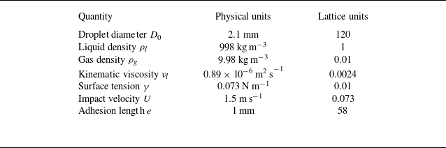


 R(t)
 e=1.0mm
 R=0

 (θL,θR)=(90∘,30∘)
 (90∘,90∘)
 (90∘,170∘)
 t1
 t2
 t3
 t4

 Ek(t)
 θL=90∘
 θR=θ
 30∘⩽θ⩽170∘
 T
 Ek,min
 θ

 Es(t)
 θL=90∘
 θR=θ
 Es( peak)
 θ

 θ
 50∘⩽θ⩽150∘

 y
 θ
 t=9400
 θ

 A(t)
 θ
 Amax
 θ

 θR=50∘
 θR=90∘
 θR=130∘
 θL=90∘
 We=80
 D=0
 E~k
 E~s
 Ξ~
 t∗
 tK∗
 tR∗
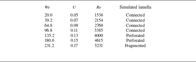
 (θL,θR)=(90∘,130∘)
 D=0
 D0=80
 ρl=1
 γ=0.01
 νl=0.0026
 Oh=2.91×10⁻³

 Ek/Ek0
 We
 We=96.8
 We=180.0
 We=231.2

 Es(t)
 We
 Es( peak)
 We

 Ξ(tR∗)

 We
 We

 We
 t=9400
 We

 A(t)
 We
 Amax
 We

 Ek(t)
 D
 D

 Es(t)
 D
 Es( peak)
 D

 D
 t=10800
 D

 y
 z
 t=10800
 D=−1
 D=0
 D=1
 (θL,θR)=(90∘,130∘)
 We=96.8

 y
 D
 ymin
 D

 A(t)
 D
 Amax
 D

 A^
 E^s
 E^k
 Ω^
 (θL,θR)=(90∘,130∘)
 We=96.8
 D=0


