1 Introduction
The linear water-wave theory for long waves indicates that, during shoaling, the wave amplitude increases at the rate of a negative one-quarter power law,
 $a\propto h^{-1/4}$
, in which
 $a$
is the wave amplitude and
 $h$
is the local water depth at the quiescent state. This is called Green’s law. Green’s law is valid for unidirectional propagating linear non-dispersive long waves with no energy dissipation. On the other hand, shoaling for a solitary wave on a mild slope beach results in amplitude growth at the rate of
 $a\propto h^{-1}$
. There are a few factors that we must recognize. First, once a solitary wave commences entering the sloping bathymetry, it no longer maintains the property of a soliton. Second, the theory assumes that the beach slope is so small that the amplitude and wavelength of a solitary wave are allowed to vary slowly while maintaining its solitary-wave formation. To support such gradual transformation, the wavelength of the solitary wave must be much shorter than the beach length. Note that this gradual transformation process is also applied to Green’s law.
The following are a couple of observations that may cast a question on the applicability of
 $a\propto h^{-1/4}$
(Green’s law) and
 $a\propto h^{-1}$
. Tsunami waveforms of the 2011 Heisei tsunami event were recorded with the GPS buoys installed offshore along the Sanriku coast (PARI 2011). One of the buoys is located approximately 15 km offshore from the city of Kamaishi at a depth of 204 m (at
 $39^{\circ }15^{\prime }31^{\prime \prime }$
N,
 $142^{\circ }05^{\prime }49^{\prime \prime }$
E). Along the same latitude (i.e. west-to-east transect line), the tsunamis were also recorded with two sea-bottom pressure transducers: one is located at approximately 45 km offshore at a water depth of 1013 m (
 $39^{\circ }14^{\prime }56^{\prime \prime }$
N,
 $142^{\circ }26^{\prime }28^{\prime \prime }$
E), and the other is at 73 km offshore at a depth of 1618 m (
 $39^{\circ }13^{\prime }52.3^{\prime \prime }$
N,
 $142^{\circ }46^{\prime }06.1^{\prime \prime }$
E). The beach slope is fairly uniform: approximately
 $\tan \unicode[STIX]{x1D703}=1/50$
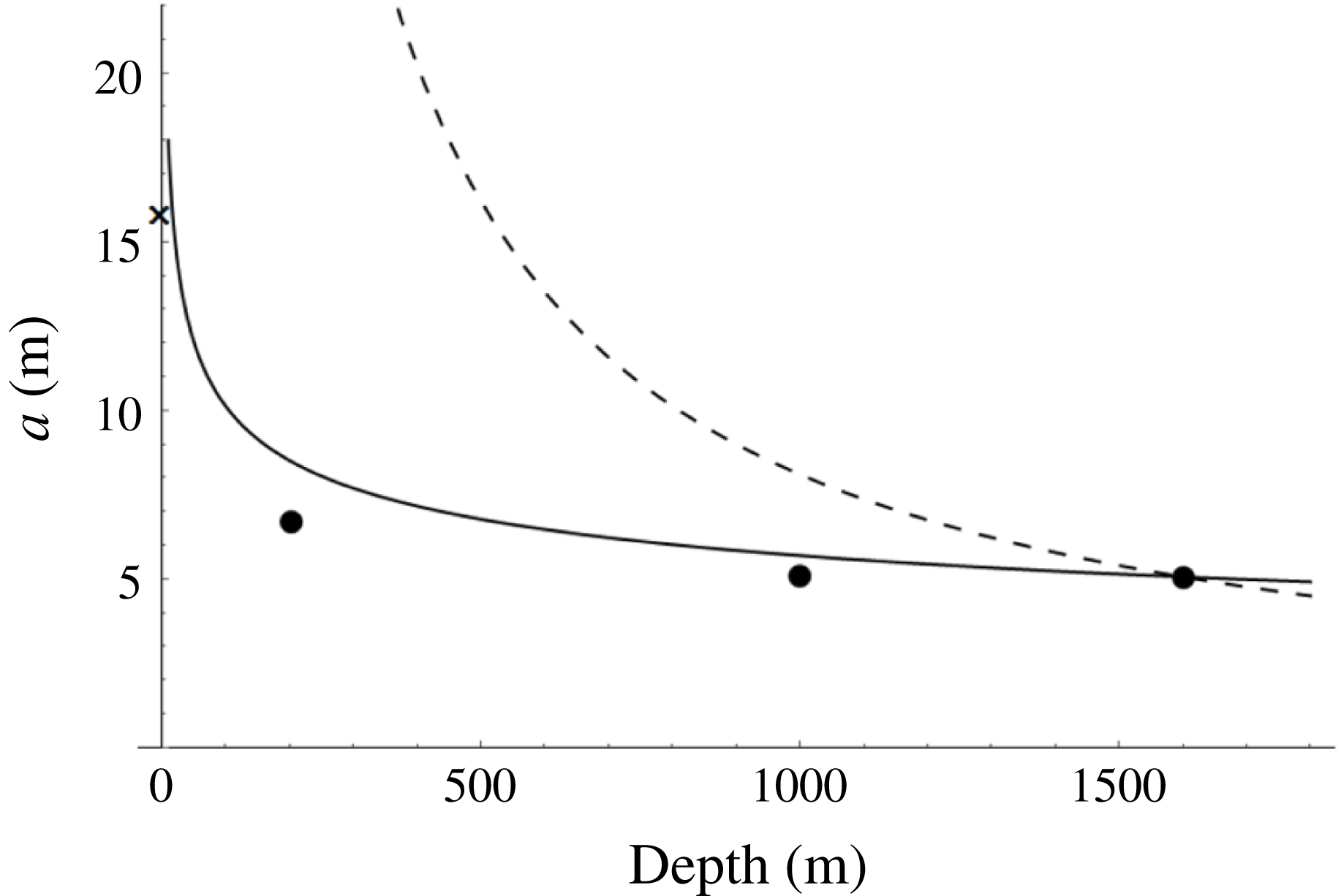
. Figure 1 shows the wave heights at the locations together with the wave height at the shore. It shows that the shoaling amplification rate is slightly slower than the prediction of Green’s law,
 $a\propto h^{-1/4}$
, and significantly slower than
 $a\propto h^{-1}$
.
Tsunami wave height versus distance along the east–west transect near
 $39^{\circ }15^{\prime }$
N. The solid line is the prediction of Green’s law,
 $a\propto h^{-1/4}$
; the dashed line represents the prediction of the growth rate
 $a\propto h^{-1}$
. The wave height at the shore marked as
 $\times$
(15.7 m) was estimated at the average of the measured run-up heights in the area adjacent to Kamaishi’s tsunami breakwater, assuming the tsunami amplification due to reflection at the shore as being doubled. For detailed information, see Yeh, Sato & Tajima (Reference Yeh, Sato, Tajima, Lee and Ng2011).

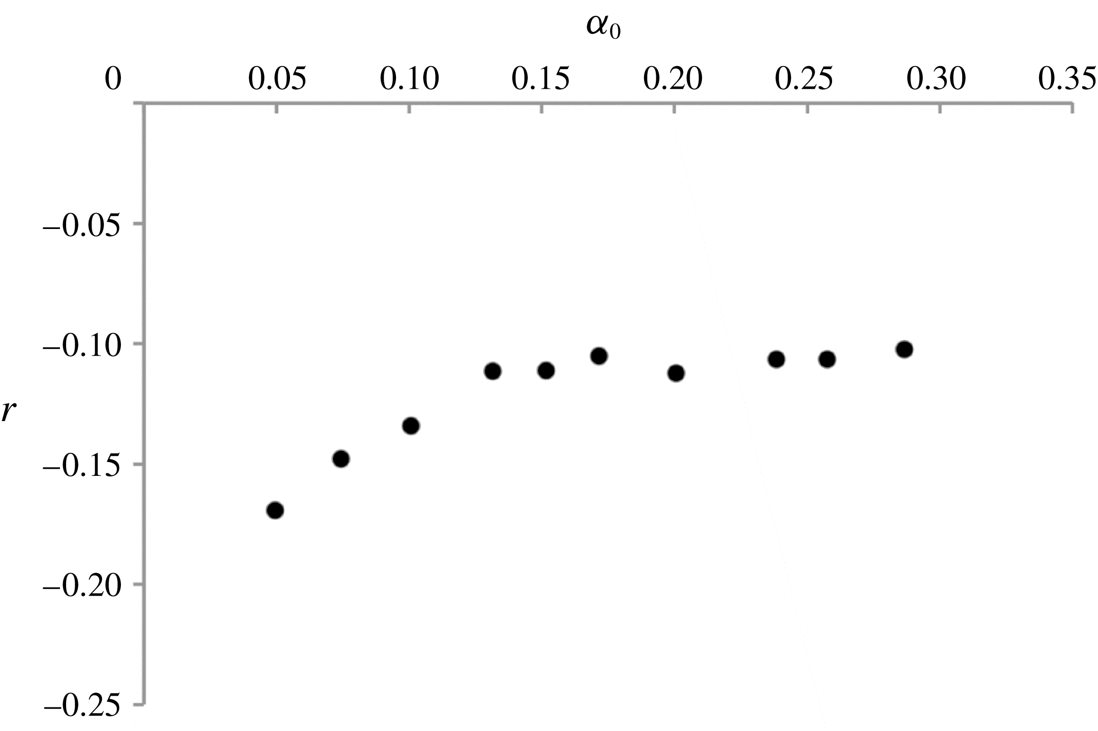
This slower growth rate was also observed by the study of Pujara, Liu & Yeh (Reference Pujara, Liu and Yeh2015), who performed laboratory experiments to generate a solitary wave in a wave flume that was 104 m long and 3.7 m wide with a water depth of 1.72 m. After propagating 23 m, the generated solitary wave climbs a plane beach of slope 1 : 12. The resulting shoaling exponent
 $r$
(
 $a\propto h^{r}$
) is plotted with the values of the nonlinearity parameter offshore
 $\unicode[STIX]{x1D6FC}_{0}\equiv a_{0}/h_{0}$
, in which
 $a_{0}$
is the solitary-wave amplitude offshore where the water depth is uniform at
 $h_{0}=1.72~\text{m}$
. Figure 2 shows that the shoaling exponent for the solitary waves is greater than that of Green’s law (
 $r>-1/4$
), which means that the amplification is slower than the prediction of Green’s law: this trend is consistent with the observation of the 2011 Heisei tsunami as shown in figure 1. In fact, the results of Pujara et al. (Reference Pujara, Liu and Yeh2015) show that, as the nonlinearity of the incident solitary wave increases, the shoaling exponent appears to approach
 $r\rightarrow -1/10$
.
The shoaling rate exponent
 $r$
based on the large-scale laboratory data by Pujara et al. (Reference Pujara, Liu and Yeh2015):
 $a\propto h^{r}$
. The offshore solitary waves are represented with the nonlinearity parameter
 $\unicode[STIX]{x1D6FC}_{0}=a_{0}/h_{0}$
. Data were taken in the deep portion of the laboratory flume where
 $0.47<h/h_{0}<1$
.

Here we present shoaling processes for localized waveforms with a variety of wavelengths, including the length being comparable to, and even longer than, the beach breadth. We choose solitary waves as the localized waves incident onto sloping bathymetry, which allows us to conveniently characterize the incident waves with two parameters: viz. amplitude and water depth. In addition, the solitary-wave’s stable and permanent-form characteristics provide us with the consistent and convenient initial condition for the study. While trivial, it is important to recognize that the beach length is always finite depending on the slope. In fact, this trivial factor is the key to understanding the shoaling of localized long waves.
2 Background
The classic linear water-wave theory reveals that, during shoaling, the wave amplitude follows a negative one-quarter power law, i.e. Green’s law – see Lamb (Reference Lamb1932, § 185) for example. Green’s law arises from the theory of unidirectional propagating linear non-dispersive long waves where the effects of friction are neglected. On the other hand, the amplification rate of shoaling for a solitary wave is proportional to the reciprocal of the local still-water depth,
 $a\propto h^{-1}$
. This shoaling process is termed ‘adiabatic’ evolution by Miles (Reference Miles1983) because it is based on the conservation of energy of a solitary wave (Miles Reference Miles1979). Under the adiabatic shoaling process, the amplitude and wavelength of a solitary wave are allowed to vary slowly while maintaining its solitary-wave form. This adiabatic shoaling process was originally predicted by Boussinesq, according to Miles (Reference Miles1983). Shuto (Reference Shuto1973) showed
 $a\propto h^{-1}$
by analysing the Kakutani equation (Kakutani Reference Kakutani1971) by setting the Ursell parameter to be unity. A different approach to this problem was presented in Miles (Reference Miles1979), where the principle of conservation of wave energy is employed to find a rate of shoaling that is in agreement with the adiabatic shoaling process. Miles found, however, that, unless the mean water level vanishes (e.g. periodic waves), the total mass cannot be contained in the main wave body but distributed to the generation of trailing and reflected residuals. This indicates that shoaling of a localized wave (i.e. an aperiodic water-surface displacement of finite extent) such as a solitary wave is different from a periodic wavetrain. Miles (Reference Miles1983) also explores the shoaling of a solitary wave with the inclusion of turbulent bottom friction by implementing Chezy’s law for a boundary layer. The result by El, Grimshaw & Kamchatnov (Reference El, Grimshaw and Kamchatnov2007) also coincides with the minus-one power law, but was attained through the averaging method outlined in Whitham (Reference Whitham1965) when applied to the variable-coefficient perturbed Korteweg–de Vries (KdV) equation (Johnson Reference Johnson1973a
,Reference Johnson
b
; Grimshaw Reference Grimshaw1981). Recently, Kalisch & Senthilkumar (Reference Kalisch and Senthilkumar2013) showed that the adiabatic shoaling evolution process is also obtained from the coupled Benjamin–Bona–Mahony (BBM) equations (Bona, Chen & Saut Reference Bona, Chen and Saut2002).
However, for periodic waves, Madsen & Sørensen (Reference Madsen and Sørensen1992) show that, based on the linearized Boussinesq equations, the shoaling amplification rate is slower than Green’s law (and of course that of the adiabatic shoaling). This trend is consistent with the observations we discussed for the field record of the 2011 Heisei tsunami (Yeh et al. Reference Yeh, Sato, Tajima, Lee and Ng2011) and the laboratory data by Pujara et al. (Reference Pujara, Liu and Yeh2015).
Ippen & Kulin (Reference Ippen and Kulin1954) reported in a laboratory study that the shoaling of a wave amplitude is proportional to the water depth by some power law,
 $a\propto h^{r}$
, with
 $r=-0.49$
,
 $-0.26$
and
 $-0.18$
for beach slopes of
 $\tan \unicode[STIX]{x1D703}=0.023$
, 0.050 and 0.065, respectively. Note that it is difficult to draw a definitive conclusion from substantial variations present in the data. The laboratory and numerical studies were performed by the Stanford University group (Street & Camfield Reference Street and Camfield1966; Camfield & Street Reference Camfield and Street1969; Chan & Street Reference Chan and Street1970). Based on the linear shallow-water-wave theory, Synolakis (Reference Synolakis1990) found an exact solution for wave run-up onto a uniformly sloping beach where the incident waveform offshore is a solitary wave. Analysing the asymptotic nature of this solution for a large distance from the shore results in shoaling that follows Green’s law, as expected because of the use of the linear shallow-water-wave equations. Synolakis’s prediction for the applicability of Green’s law is demonstrated experimentally in the laboratory by Synolakis & Skjelbreia (Reference Synolakis and Skjelbreia1993): the laboratory experiments were performed with a beach slope of
 $\tan \unicode[STIX]{x1D703}=1/52$
. Their laboratory observation near the shore shows that the wave shoals in accordance with the adiabatic evolution process (i.e.
 $a\propto h^{-1}$
). In other words, the rate of shoaling agrees with Green’s law at the commencement of wave run-up near the beach toe, but, after the wave has climbed the beach for some time, the rate of shoaling increases and is better predicted by the adiabatic assumption. This two-zone model for solitary-wave shoaling was suggested earlier by Shuto (Reference Shuto1973), who analysed the laboratory data given by Street & Camfield (Reference Street and Camfield1966) and Camfield & Street (Reference Camfield and Street1969). Experimental results by Hsiao et al. (Reference Hsiao, Hsu, Lin and Chang2008) appear to display this ‘two-zone’ model: they used a beach with a slope of
 $\tan \unicode[STIX]{x1D703}=1/60$
.
Peregrine (Reference Peregrine1967) extended the Boussinesq equations for a uniformly sloping beach, and derived the often called Peregrine equations. His numerical predictions based on the Peregrine equations yield reasonable approximation to Green’s law. Grilli et al. (Reference Grilli, Subramanya, Svendsen and Veeramony1994) numerically computed the full Euler formulation by transforming it into a boundary-integral equation. Their numerical results are validated with their laboratory experiments, and show that, when the beach slope is very mild, the results are qualitatively in agreement with the ‘two-zone’ shoaling model (Green’s law
 $\rightarrow$
adiabatic evolution) as proposed by Shuto (Reference Shuto1973) and later by Synolakis & Skjelbreia (Reference Synolakis and Skjelbreia1993).
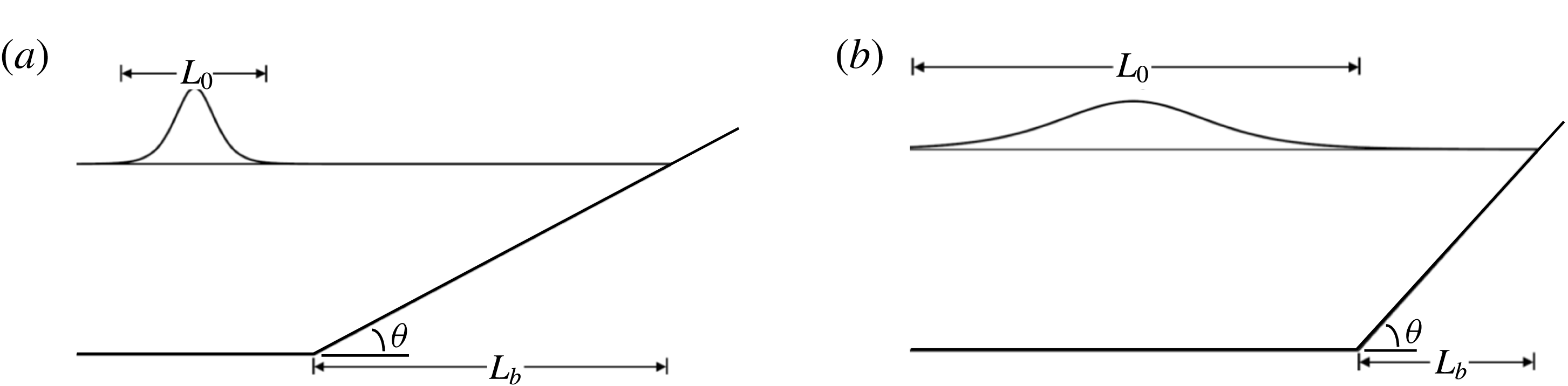
Two sketches to depict the extreme shoaling scenarios (the solitary waves shown here are not scaled): (a) the beach scale is much larger than the wave scale,
 $L_{b}\gg L_{0}$
; (b) the beach scale is much smaller than the wave scale,
 $L_{b}\ll L_{0}$
.

3 Preliminary considerations
An incoming solitary wave with amplitude
 $a_{0}$
propagating in a uniform water depth
 $h_{0}$
can be written as
 $$\begin{eqnarray}\tilde{\unicode[STIX]{x1D702}}\simeq a_{0}\,\text{sech}^{2}\sqrt{\frac{3a_{0}}{4h_{0}^{3}}}\left[\tilde{x}-c_{0}\left(1+\frac{a_{0}}{2h_{0}}\right)\tilde{t}\right].\end{eqnarray}$$
Here
 $\tilde{\unicode[STIX]{x1D702}}$
is the water surface displacement,
 $c_{0}=\sqrt{gh_{0}}$
is the phase speed of the equivalent linear long wave, and
 $\tilde{x}$
and
 $\tilde{t}$
represent the propagation distance and time, respectively. We consider the case where a solitary wave approaches the beach toe and climbs up onto a plane beach inclined at an angle
 $\unicode[STIX]{x1D703}$
. The horizontal length scale of a solitary wave is
 $$\begin{eqnarray}L_{0}=h_{0}\sqrt{4h_{0}/3a_{0}}.\end{eqnarray}$$
Note that
 $L_{0}$
is not arbitrary, but once the wave amplitude and the water depth are given, then the value of
 $L_{0}$
is uniquely determined. We recognize that there is another length scale involved in the present problem, i.e. the horizontal length scale of the beach:
 $$\begin{eqnarray}L_{b}=h_{0}/\tan \unicode[STIX]{x1D703}.\end{eqnarray}$$
Consider a solitary wave with a large amplitude climbing onto a beach with a very mild slope, i.e.
 $L_{0}\ll L_{b}$
(see figure 3
a). In this situation, the solitary wave has a sufficient (but finite) propagation distance (or time) to evolve. Hence, it is anticipated that the evolution could be approximated by a slowly varying solitary wave maintaining that wave energy is conserved. In other words, the adiabatic evolution process is probable. However, because the nonlinearity of the incident wave is sufficiently large for small
 $L_{0}$
, the incident wave is likely to break soon after it enters the beach.
When a solitary wave with a small amplitude (i.e. large wavelength
 $L_{0}$
) approaches a beach with steep slope (small
 $L_{b}$
), the wave as a whole may not be able to shoal on the beach because of the short beach distance in comparison to the wavelength (see figure 3
b). In other words, the wavelength is too long so that only a portion of the waveform may be influenced by the beach. In this case, we anticipate little shoaling, although the wave should be amplified by reflection from the steep beach.
It is recognized that the propagation domain on the sloping bed is finite and limited by the shoreline. The steeper the slope, the shorter the available propagation distance. Therefore the parameter
 $$\begin{eqnarray}\unicode[STIX]{x1D6FE}\equiv \frac{L_{0}}{L_{b}}=\sqrt{\frac{4\tan ^{2}\unicode[STIX]{x1D703}}{3\unicode[STIX]{x1D6FC}_{0}}}\end{eqnarray}$$
must be relevant in characterizing the shoaling process, where
 $\unicode[STIX]{x1D6FC}_{0}=a_{0}/h_{0}$
. Note that the parameter
 $\unicode[STIX]{x1D6FE}$
is similar to the solitary-wave slope parameter that was proposed by Grilli, Svendsen & Subramanya (Reference Grilli, Svendsen and Subramanya1997) for their study on wave breaking of solitary waves. We also note that the parameter
 $\unicode[STIX]{x1D6FE}$
resembles the Iribarren number (or the surf similarity parameter) often used for modelling effects of breaking waves on beaches (see e.g. Bowen, Inman & Simons Reference Bowen, Inman and Simons1968; Battjes Reference Battjes1974). The Iribarren number (
 $\unicode[STIX]{x1D709}=\tan \unicode[STIX]{x1D703}/\sqrt{H_{0}/\unicode[STIX]{x1D706}_{0}}$
) represents the ratio of beach slope to wave nonlinearity
 $H_{0}/\unicode[STIX]{x1D706}_{0}$
, where
 $H_{0}$
is the wave height and
 $\unicode[STIX]{x1D706}_{0}$
is the wavelength of the incident waves in deep water. On the other hand, the beach slope parameter
 $\unicode[STIX]{x1D6FE}$
in (3.4) expresses a more concrete physical meaning: viz. the length-scale ratio of the solitary wave to the beach.
In short, when
 $\unicode[STIX]{x1D6FE}=L_{0}/L_{b}\ll 1$
, we anticipate that the solitary wave has a sufficient propagation distance on the beach, allowing itself to adjust in order to maintain its soliton identity during shoaling. On the other hand, when
 $\unicode[STIX]{x1D6FE}\gg 1$
, the incoming solitary wave would be too long, so that only a small portion of the waveform is influenced (if any) by the beach: for a very steep slope, one could consider the process resembling wave reflection at a vertical wall.
4 Theoretical considerations
Here we discuss the effects of nonlinearity
 $(\unicode[STIX]{x1D6FC}_{0}=a_{0}/h_{0})$
, frequency dispersion
 $(\unicode[STIX]{x1D6FD}_{0}=(h_{0}/L_{0})^{2})$
and beach slope
 $(\tan \unicode[STIX]{x1D703})$
on the evolution of a solitary wave on a uniformly sloping beach in terms of the variable-coefficient perturbed Korteweg–de Vries (vKdV) equation (e.g. Johnson Reference Johnson1973a
,Reference Johnson
b
; Grimshaw Reference Grimshaw1981). The friction effect is ignored, so the equation can be written in the following homogeneous form:
 $$\begin{eqnarray}\tilde{\unicode[STIX]{x1D702}}_{\tilde{t}}+\tilde{c}\tilde{\unicode[STIX]{x1D702}}_{\tilde{x}}+\frac{\tilde{c}_{\tilde{x}}}{2}\tilde{\unicode[STIX]{x1D702}}+\frac{3\tilde{c}}{2\tilde{h}}\tilde{\unicode[STIX]{x1D702}}\tilde{\unicode[STIX]{x1D702}}_{\tilde{x}}+\frac{\tilde{c}\tilde{h}^{2}}{6}\tilde{\unicode[STIX]{x1D702}}_{\tilde{x}\tilde{x}\tilde{x}}=0,\quad \tilde{c}(\tilde{x})=\sqrt{g\tilde{h}(\tilde{x})}.\end{eqnarray}$$
Note that the still-water depth
 $\tilde{h}$
and the wave celerity
 $\tilde{c}$
for linear long waves are functions of the position
 $\tilde{x}$
. To study the extrema of the surface displacement
 $\tilde{\unicode[STIX]{x1D702}}$
at an arbitrary location, we set
 $\tilde{\unicode[STIX]{x1D702}}_{\tilde{t}}=0$
and substitute in the wave celerity
 $\tilde{c}$
to obtain
 $$\begin{eqnarray}\tilde{h}\tilde{\unicode[STIX]{x1D702}}_{\tilde{x}}+\frac{1}{4}\tilde{h}_{\tilde{x}}\tilde{\unicode[STIX]{x1D702}}+\frac{3}{2}\tilde{\unicode[STIX]{x1D702}}\tilde{\unicode[STIX]{x1D702}}_{\tilde{x}}+\frac{\tilde{h}^{3}}{6}\unicode[STIX]{x1D702}_{\tilde{x}\tilde{x}\tilde{x}}=0.\end{eqnarray}$$
A similar approach was used by Shuto (Reference Shuto1973) to demonstrate the ‘two-zone’ shoaling law (Green’s law
 $\rightarrow$
adiabatic evolution) for a solitary wave.
The ansatz is made that
 $\tilde{\unicode[STIX]{x1D702}}=\tilde{a}(\tilde{h}(\tilde{x}))$
, where
 $\tilde{h}(\tilde{x})=h_{0}-\tilde{x}\tan \unicode[STIX]{x1D703}$
and
 $\tilde{x}$
points in the onshore direction. Expressing
 $\tilde{\unicode[STIX]{x1D702}}$
as a function of
 $\tilde{h}$
simplifies the expression (4.2) to the following third-order nonlinear ordinary differential equation (ODE):
 $$\begin{eqnarray}\tilde{h}\tilde{a}^{\prime }(\tilde{h})+\frac{1}{4}\tilde{a}(\tilde{h})+\frac{3}{2}\tilde{a}(\tilde{h})\tilde{a}^{\prime }(\tilde{h})+\frac{\tan ^{2}\unicode[STIX]{x1D703}}{6}\tilde{h}^{3}\tilde{a}^{\prime \prime \prime }(\tilde{h})=0.\end{eqnarray}$$
This is rewritten in terms of non-dimensional variables:
 $$\begin{eqnarray}\tilde{a}=a_{0}a,\quad \tilde{h}=h_{0}h.\end{eqnarray}$$
Then (4.3) is expressed as
 $$\begin{eqnarray}ha^{\prime }(h)+\frac{1}{4}a(h)+\unicode[STIX]{x1D6FC}_{0}\frac{3}{2}a(h)a^{\prime }(h)+\frac{\tan ^{2}\unicode[STIX]{x1D703}}{6}h^{3}a^{\prime \prime \prime }(h)=0.\end{eqnarray}$$
It should be noted that the order of magnitude of the nonlinear effect in (4.5) is represented by the parameter
 $\unicode[STIX]{x1D6FC}_{0}$
and the order of magnitude of the frequency-dispersion effect is expressed by
 $h^{3}\tan ^{2}\unicode[STIX]{x1D703}$
. In other words, the dispersion becomes more important in the deeper portion of the beach (near the beach toe) and when the beach slope is steep, although the vKdV equation requires the beach slope to be small. We will now examine the cases where certain terms from (4.5) are neglected.
4.1 Case 1 – linear and non-dispersive
The effects of frequency dispersion and nonlinearity are neglected in (4.5). Note that it is not necessary to choose
 $h(x)$
to be a linear function of
 $x$
in order to arrive at the following equation:
 $$\begin{eqnarray}ha^{\prime }(h)+{\textstyle \frac{1}{4}}a(h)=0.\end{eqnarray}$$
This is a linear first-order ODE that can be solved by standard methods of integration. The solution is given by
 $$\begin{eqnarray}a(h)=C_{0}h^{-1/4},\end{eqnarray}$$
where
 $C_{0}$
is a constant of integration. This is the well-known result referred to as Green’s law and now resulted from the vKdV equation.
4.2 Case 2 – linear and dispersive
Now let us examine the effects of frequency dispersion, which allows us to examine how the beach slope affects the rate of shoaling. The nonlinear term from (4.5) is neglected to yield
 $$\begin{eqnarray}\frac{\tan ^{2}\unicode[STIX]{x1D703}}{6}h^{3}a^{\prime \prime \prime }(h)+ha^{\prime }(h)+\frac{1}{4}a(h)=0.\end{eqnarray}$$
This is a third-order Euler-type equation that can be solved by
 $a(h)=C_{0}h^{r}$
, where
 $r$
is given by the roots of the following cubic polynomial:
 $$\begin{eqnarray}\tan ^{2}\unicode[STIX]{x1D703}({\textstyle \frac{1}{6}}r^{3}-{\textstyle \frac{1}{2}}r^{2}+{\textstyle \frac{1}{3}}r)+r+{\textstyle \frac{1}{4}}=0.\end{eqnarray}$$
The negative real root corresponds to the physical solution. Note that, for small slopes, the root would become
 $r=-1/4$
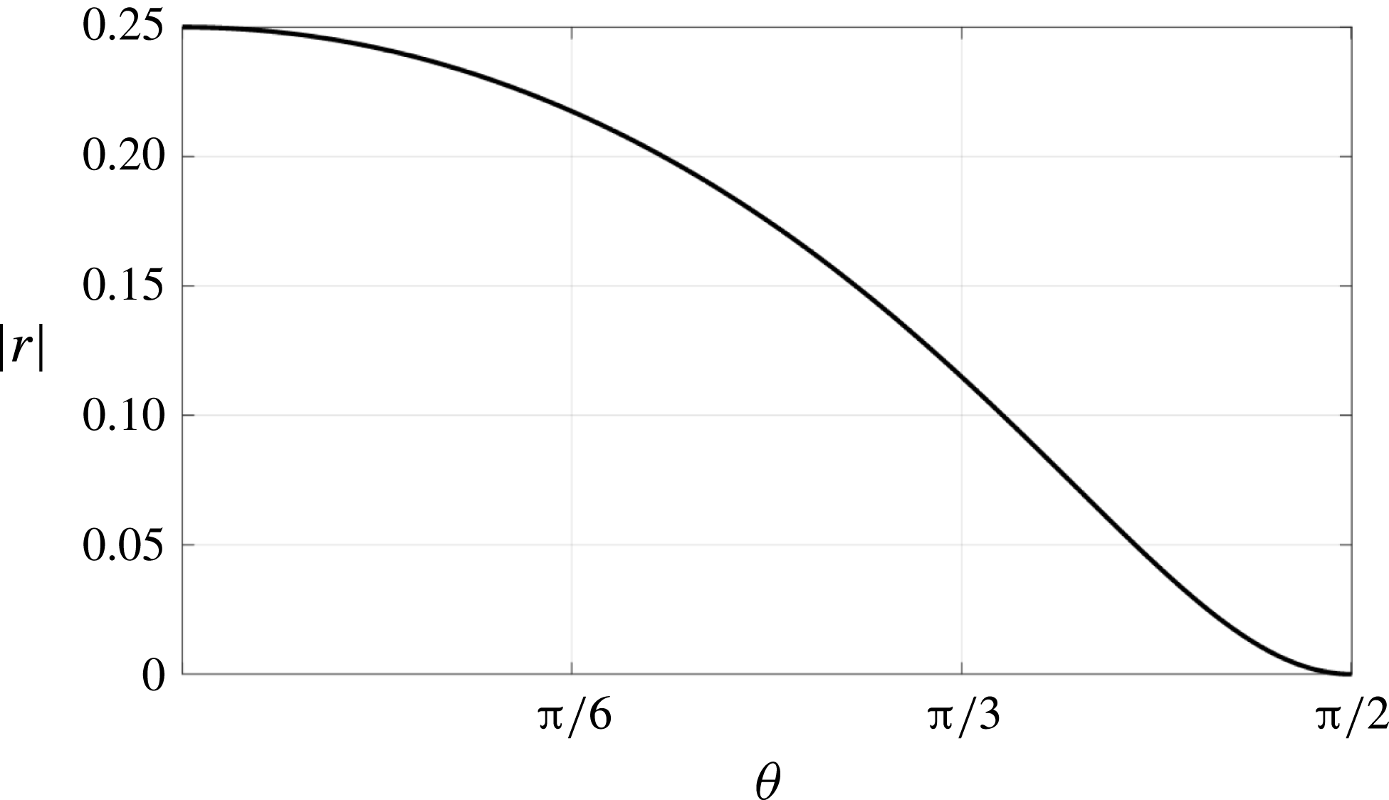
, which reverts back to Green’s law. As the beach slope increases, the absolute value of the shoaling exponent
 $r$
monotonically decreases to zero, as seen in figure 4. This decreasing trend in the absolute value of
 $r$
from 1/4 appears to agree qualitatively with experiments by Ippen & Kulin (Reference Ippen and Kulin1954) and Grilli et al. (Reference Grilli, Subramanya, Svendsen and Veeramony1994), and is also consistent with the prediction for periodic waves based on the linearized Boussinesq equations by Madsen & Sørensen (Reference Madsen and Sørensen1992). When the angle of inclination is
 $\unicode[STIX]{x1D703}\approx \unicode[STIX]{x03C0}/3$
(very steep),
 $r\approx -1/10$
. In fact, Green’s law rules in typical continental shelf conditions, i.e. even when
 $\tan \unicode[STIX]{x1D703}\approx 1/4$
(steep),
 $r\approx -0.24$
.
Shoaling exponent rate (
 $a\propto h^{-|r|}$
) versus the angle of inclination
 $\unicode[STIX]{x1D703}$
(radians) based on the vKdV theory neglecting the nonlinear effect.

4.3 Case 3 – nonlinear and non-dispersive
Here we assume that frequency dispersion is negligible so that (4.5) may be reduced to the following nonlinear first-order ODE:
 $$\begin{eqnarray}ha^{\prime }(h)+{\textstyle \frac{1}{4}}a(h)+{\textstyle \frac{3}{2}}\unicode[STIX]{x1D6FC}_{0}a(h)a^{\prime }(h)=0.\end{eqnarray}$$
Note that this equation is no longer a function of the angle of inclination
 $\unicode[STIX]{x1D703}$
. This equation can be rearranged as
 $$\begin{eqnarray}a^{\prime }=\frac{-1/4}{(a/h)^{-1}+{\textstyle \frac{3}{2}}\unicode[STIX]{x1D6FC}_{0}}.\end{eqnarray}$$
Taking
 $a=hv(h)$
so that
 $a^{\prime }=v(h)+hv^{\prime }(h)$
yields
 $$\begin{eqnarray}\frac{1+{\textstyle \frac{3}{2}}\unicode[STIX]{x1D6FC}_{0}v}{v({\textstyle \frac{5}{4}}+{\textstyle \frac{3}{2}}\unicode[STIX]{x1D6FC}_{0}v)}\,\text{d}v=-\frac{1}{h}\,\text{d}h.\end{eqnarray}$$
Integration yields
 $$\begin{eqnarray}\left(\frac{a}{h}\right)^{4/5}\left(\unicode[STIX]{x1D6FC}_{0}\frac{a}{h}+\frac{5}{6}\right)^{1/5}=C_{0}h^{-1}.\end{eqnarray}$$
Note that (4.13) reduces to Green’s law when
 $\unicode[STIX]{x1D6FC}_{0}\rightarrow 0$
.
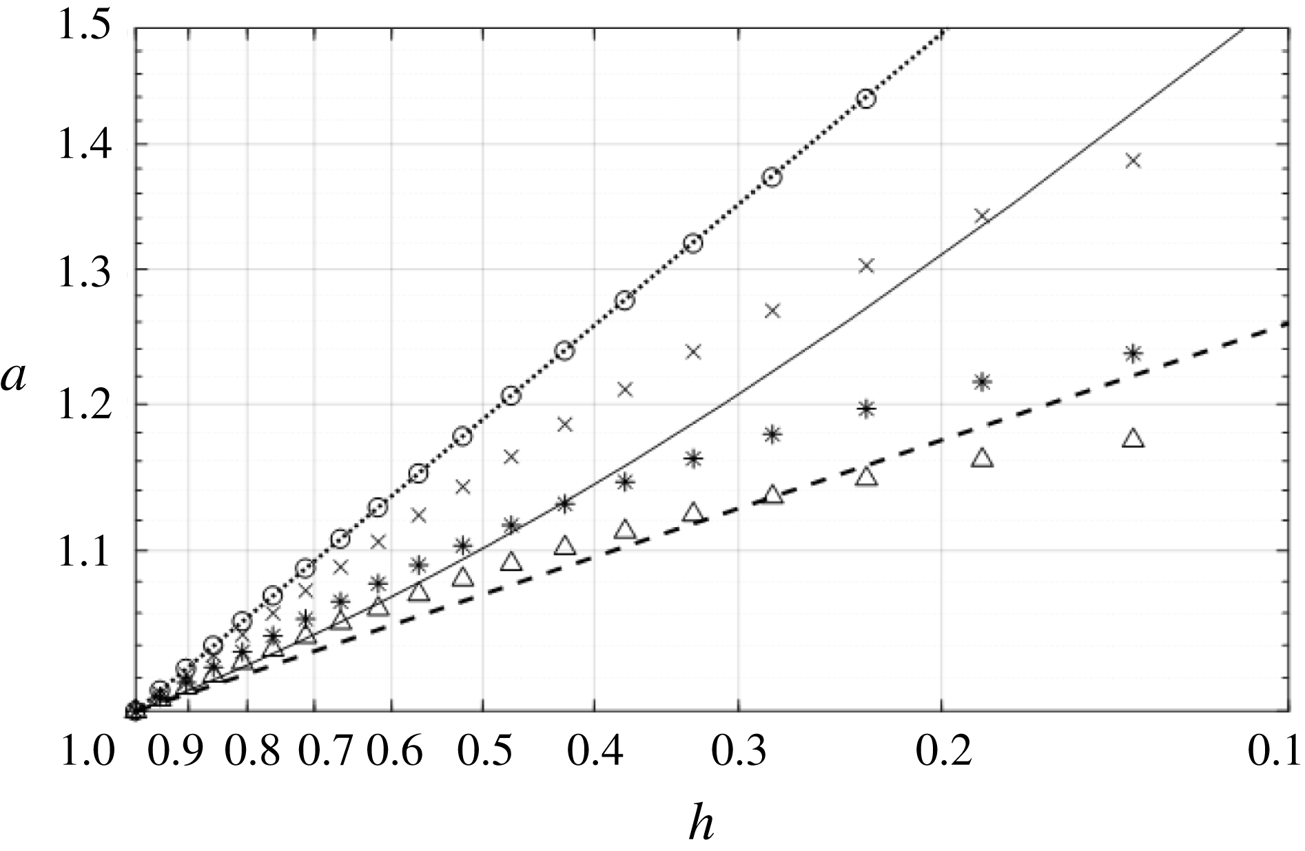
In figure 5, the solution is plotted for various values of the initial nonlinearity parameter
 $\unicode[STIX]{x1D6FC}_{0}$
. The thin solid line in figure 5 represents the wave breaking criterion for solitary waves based on
 $$\begin{eqnarray}a_{b}=\frac{0.78}{\unicode[STIX]{x1D6FC}_{0}}h_{b}.\end{eqnarray}$$
This is a theoretical prediction by McCowan (Reference McCowan1891) for a solitary wave propagating over a horizontal bed. Solitary waves above the thin solid line mean that the waves have not yet broken. The breaking depth
 $h_{b}$
can be found from (4.13) as a function of the initial nonlinearity and is given by
 $$\begin{eqnarray}h_{b}=\left(\frac{\unicode[STIX]{x1D6FC}_{0}}{0.78}\right)^{4/5}\left(\frac{\unicode[STIX]{x1D6FC}_{0}+{\textstyle \frac{5}{6}}}{0.78+{\textstyle \frac{5}{6}}}\right)^{1/5}.\end{eqnarray}$$
It can be seen in figure 5 that the solution appears to approach the rate of shoaling with the exponent
 $r\rightarrow -1/10$
for increasing values of the nonlinearity parameter before wave breaking occurs. At the same time, we see that the shoaling for the nonlinear case does not follow a power law so that a rate of shoaling is not always clearly defined.
Amplitude increase due to solitary-wave shoaling based on the vKdV theory neglecting the frequency dispersion effect: ○,
 $\unicode[STIX]{x1D6FC}_{0}=0.001$
;
 $\times$
,
 $\unicode[STIX]{x1D6FC}_{0}=0.1$
; *,
 $\unicode[STIX]{x1D6FC}_{0}=0.3$
; ▵,
 $\unicode[STIX]{x1D6FC}_{0}=0.5$
; dotted line, Green’s law; dashed line,
 $r=-1/10$
; solid line, wave breaking condition (4.14). For small values of
 $\unicode[STIX]{x1D6FC}_{0}$
, the rate of shoaling approaches Green’s law. For increasing values of
 $\unicode[STIX]{x1D6FC}_{0}$
, the rate of shoaling approaches
 $-1/10$
.

5 Numerical simulations
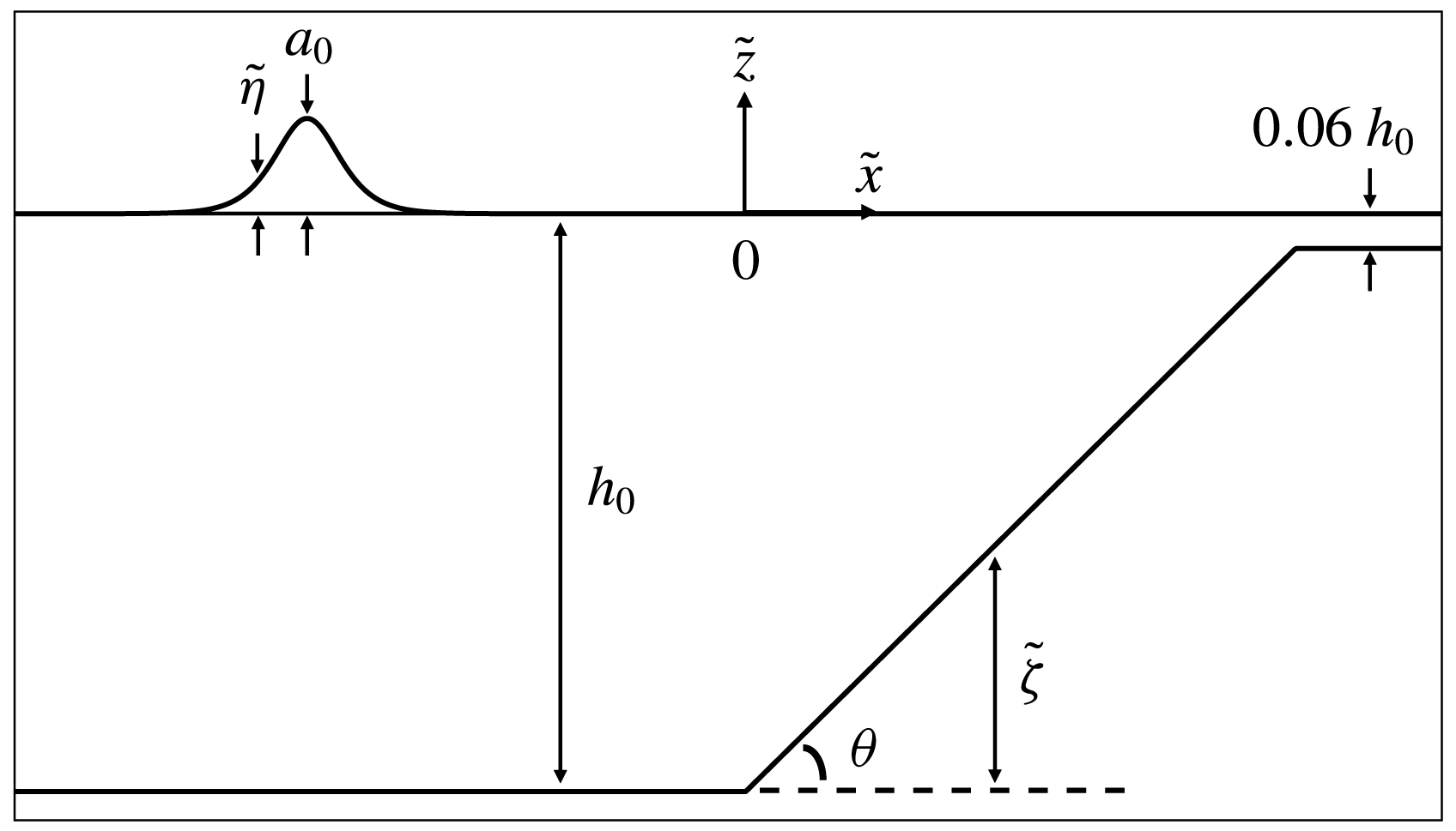
Numerical computations are conducted using a higher-order pseudo-spectral method developed by Dommermuth & Yue (Reference Dommermuth and Yue1987) for the computational domain shown in figure 6. The coordinate origin is set at the water surface over the toe of the beach; the horizontal coordinate
 $\tilde{x}$
points in the onshore direction, and
 $\tilde{z}$
points upwards. A solitary wave with amplitude
 $a_{0}$
originates offshore in quiescent water depth of
 $h_{0}$
and climbs a beach inclined at angle
 $\unicode[STIX]{x1D703}$
. The departure from the quiescent water level is denoted by
 $\tilde{\unicode[STIX]{x1D702}}$
, whereas
 $\tilde{\unicode[STIX]{x1D701}}$
is the vertical beach-bed location measured from
 $\tilde{z}=-h_{0}$
. For stability reasons inherited in the numerical method, we set a water depth of
 $0.06h_{0}$
over the inshore plateau; consequently, no wave run-up motion on a dry beach is modelled.
Definition sketch for numerical experiments.

5.1 Formulation
The full water-wave formulation of the Euler theory can be written in the non-dimensionalized form as
 $$\begin{eqnarray}\left.\begin{array}{@{}c@{}}\begin{array}{@{}c@{}}\quad \qquad \unicode[STIX]{x1D6FD}_{0}\unicode[STIX]{x1D6F7}_{xx}+\unicode[STIX]{x1D6F7}_{zz}=0\qquad \,\text{for }-1+\unicode[STIX]{x1D701}\leqslant z\leqslant \unicode[STIX]{x1D6FC}_{0}\unicode[STIX]{x1D702},\\ \unicode[STIX]{x1D6FD}_{0}\unicode[STIX]{x1D701}_{x}\unicode[STIX]{x1D6F7}_{x}-\unicode[STIX]{x1D6F7}_{z}=0\qquad \text{at }z=-1+\unicode[STIX]{x1D701},\\ \end{array}\\ \left.\begin{array}{@{}r@{}}\displaystyle \unicode[STIX]{x1D6FD}_{0}\unicode[STIX]{x1D702}_{t}+\unicode[STIX]{x1D6FC}_{0}\unicode[STIX]{x1D6FD}_{0}\unicode[STIX]{x1D6F7}_{x}^{S}\unicode[STIX]{x1D702}_{x}-(1+\unicode[STIX]{x1D6FC}_{0}^{2}\unicode[STIX]{x1D6FD}_{0}\unicode[STIX]{x1D702}_{x}^{2})\unicode[STIX]{x1D6F7}_{z}=0\,\\ \displaystyle \unicode[STIX]{x1D6FD}_{0}\unicode[STIX]{x1D6F7}_{t}^{S}+\unicode[STIX]{x1D6FD}_{0}\unicode[STIX]{x1D702}+{\textstyle \frac{1}{2}}\unicode[STIX]{x1D6FC}_{0}\unicode[STIX]{x1D6FD}_{0}(\unicode[STIX]{x1D6F7}_{x}^{S})^{2}-{\textstyle \frac{1}{2}}\unicode[STIX]{x1D6FC}_{0}(1+\unicode[STIX]{x1D6FC}_{0}^{2}\unicode[STIX]{x1D6FD}_{0}\unicode[STIX]{x1D702}_{x}^{2})\unicode[STIX]{x1D6F7}_{z}^{2}=0\,\end{array}\right\}\quad \text{at }z=\unicode[STIX]{x1D6FC}_{0}\unicode[STIX]{x1D702},\end{array}\right\}\end{eqnarray}$$
where
 $\unicode[STIX]{x1D6F7}(x,z,t)$
is the velocity potential,
 $\unicode[STIX]{x1D6F7}^{S}(x,t)=\unicode[STIX]{x1D6F7}(x,t,z=\unicode[STIX]{x1D702}(x,t))$
is the velocity potential evaluated at the free surface,
 $\unicode[STIX]{x1D6FC}_{0}=a_{0}/h_{0}$
is the nonlinearity parameter,
 $\unicode[STIX]{x1D6FD}_{0}=(h_{0}/L_{0})^{2}$
is the dispersion parameter, and the other parameters are normalized by
 $$\begin{eqnarray}x=\frac{\tilde{x}}{L_{0}},\quad z=\frac{\tilde{z}}{h_{0}},\quad t=\frac{c_{0}}{L_{0}}\tilde{t},\quad \unicode[STIX]{x1D702}=\frac{\tilde{\unicode[STIX]{x1D702}}}{a_{0}},\quad \unicode[STIX]{x1D6F7}=\frac{h_{0}}{a_{0}L_{0}c_{0}}\tilde{\unicode[STIX]{x1D6F7}},\quad \unicode[STIX]{x1D701}=\frac{\tilde{\unicode[STIX]{x1D701}}}{h_{0}},\end{eqnarray}$$
where
 $c_{0}=\sqrt{gh_{0}}$
, and the parameters with a tilde represent the corresponding dimensional quantities as depicted in figure 6. The model assumes the irrotational flow of an inviscid, homogeneous, incompressible fluid. Note that the formulation (5.1) is often called the Zakharov–Craig–Sulem formulation after Zakharov (Reference Zakharov1968) and Craig & Sulem (Reference Craig and Sulem1993).
The horizontal gradients of
 $\unicode[STIX]{x1D6F7}^{S}$
and
 $\unicode[STIX]{x1D702}$
in (5.1) can be evaluated at the free surface through the algebraic derivative by means of the fast Fourier transform (FFT). However, the vertical velocity must be computed, which is accomplished through the implementation of an asymptotic expansion.
With the use of a Taylor-series expansion about
 $z=0$
, the perturbation expansion of the velocity potential at the free surface is given by
 $$\begin{eqnarray}\unicode[STIX]{x1D6F7}(x,z=\unicode[STIX]{x1D702},t)=\unicode[STIX]{x1D6F7}^{S}(x,t)=\mathop{\sum }_{m=1}^{M}\mathop{\sum }_{k=0}^{M-m}\unicode[STIX]{x1D716}^{m}\frac{\unicode[STIX]{x1D702}^{k}}{k!}\left.\frac{\unicode[STIX]{x2202}^{k}\unicode[STIX]{x1D719}_{m}}{\unicode[STIX]{x2202}z^{k}}\right|_{(x,z=0,t)},\end{eqnarray}$$
where
 $\unicode[STIX]{x1D716}\ll \mathit{O}(1)$
is a small perturbation parameter. It is assumed that
 $\unicode[STIX]{x1D6FC}_{0}$
and
 $\unicode[STIX]{x1D6FD}_{0}$
are of the order
 $\mathit{O}(\unicode[STIX]{x1D716})$
. Following Dommermuth & Yue (Reference Dommermuth and Yue1987),
 $\unicode[STIX]{x1D719}_{m}$
can be expressed as
 $$\begin{eqnarray}\unicode[STIX]{x1D719}_{m}(x,z,t)=A_{m}(x,z,t)+B_{m}(x,z,t),\end{eqnarray}$$
in which
 $$\begin{eqnarray}\displaystyle & \displaystyle A_{m}(x,z,t)=\mathop{\sum }_{n=1}^{N}A_{m,n}(t)\frac{\cosh k_{n}\sqrt{\unicode[STIX]{x1D6FD}_{0}}(z+1)}{\cosh (k_{n}\sqrt{\unicode[STIX]{x1D6FD}_{0}})}\text{e}^{\text{i}k_{n}x}, & \displaystyle\end{eqnarray}$$
 $$\begin{eqnarray}\displaystyle & \displaystyle B_{m}(x,z,t)=B_{m,0}(t)\sqrt{\unicode[STIX]{x1D6FD}_{0}}z+\mathop{\sum }_{n=1}^{N}B_{m,n}(t)\frac{\sinh k_{n}\sqrt{\unicode[STIX]{x1D6FD}_{0}}z}{k_{n}\cosh (k_{n}\sqrt{\unicode[STIX]{x1D6FD}_{0}})}\text{e}^{\text{i}k_{n}x}. & \displaystyle\end{eqnarray}$$
The vertical velocity
 $(w=\unicode[STIX]{x1D6F7}_{z})$
at the free surface can be expressed as
 $$\begin{eqnarray}w(x,\unicode[STIX]{x1D702},t)=\mathop{\sum }_{m=1}^{M}\mathop{\sum }_{k=0}^{M-m}\unicode[STIX]{x1D716}^{m}\frac{\unicode[STIX]{x1D702}^{k}}{k!}\left.\frac{\unicode[STIX]{x2202}^{k+1}(A_{m}+B_{m})}{\unicode[STIX]{x2202}z^{k+1}}\right|_{(x,z=0,t)}.\end{eqnarray}$$
Combining (5.3) and (5.4) we equate terms of like order to yield the sequence of
 $A_{m}$
at
 $z=0$
:
 $$\begin{eqnarray}\left.\begin{array}{@{}l@{}}A_{1}=\unicode[STIX]{x1D6F7}^{S},\\ A_{2}=-\unicode[STIX]{x1D702}(A_{1}+B_{1})_{z},\\ A_{3}=-\unicode[STIX]{x1D702}(A_{2}+B_{2})_{z}-{\displaystyle \frac{\unicode[STIX]{x1D702}^{2}}{2!}}(A_{1})_{zz},\\ A_{4}=-\unicode[STIX]{x1D702}(A_{3}+B_{3})_{z}-{\displaystyle \frac{\unicode[STIX]{x1D702}^{2}}{2!}}(A_{2})_{zz}-{\displaystyle \frac{\unicode[STIX]{x1D702}^{3}}{3!}}(A_{1}+B_{1})_{zzz},\\ A_{5}=-\unicode[STIX]{x1D702}(A_{4}+B_{4})_{z}-{\displaystyle \frac{\unicode[STIX]{x1D702}^{2}}{2!}}(A_{3})_{zz}-{\displaystyle \frac{\unicode[STIX]{x1D702}^{3}}{3!}}(A_{2}+B_{2})_{zzz}-{\displaystyle \frac{\unicode[STIX]{x1D702}^{4}}{4!}}(A_{1})_{zzzz}.\end{array}\right\}\end{eqnarray}$$
In addition, the velocity potential must satisfy the kinematic boundary condition at the bed:
 $$\begin{eqnarray}\unicode[STIX]{x1D6FD}_{0}\unicode[STIX]{x1D701}_{x}\unicode[STIX]{x1D6F7}_{x}-\unicode[STIX]{x1D6F7}_{z}=0,\quad z=-1+\unicode[STIX]{x1D701}(x).\end{eqnarray}$$
Just like our treatment made for the boundary condition at the water surface, the velocity potential is then expanded about
 $z=-1$
in order to obtain an expression suitable for substitution into the bottom boundary condition:
 $$\begin{eqnarray}\unicode[STIX]{x1D6F7}(x,z=-1+\unicode[STIX]{x1D701},t)=\mathop{\sum }_{m=1}^{M}\mathop{\sum }_{k=0}^{M-m}\unicode[STIX]{x1D716}^{m}\frac{\unicode[STIX]{x1D701}^{k}}{k!}\left.\frac{\unicode[STIX]{x2202}^{k}(A_{m}+B_{m})}{\unicode[STIX]{x2202}z^{k}}\right|_{(x,z=-1,t)}.\end{eqnarray}$$
Upon substitution and equating like-order terms, we find the sequence of
 $B_{m}$
at
 $z=-1$
. At the lowest term, we find
 $(B_{1})_{z}=0$
. With (5.6), this indicates that the value of
 $B_{1}$
identically vanishes; hence all
 $B_{1}$
terms in (5.8) also vanish. The rest of the sequence becomes
 $$\begin{eqnarray}\left.\begin{array}{@{}rcl@{}}(B_{2})_{z}\,\, & =\,\, & \unicode[STIX]{x1D701}_{x}(A_{1})_{x}-\unicode[STIX]{x1D701}(A_{1})_{zz},\\ (B_{3})_{z}\,\, & =\,\, & \unicode[STIX]{x1D701}_{x}(A_{2}+B_{2})_{x}-\unicode[STIX]{x1D701}(A_{2}+B_{2})_{zz},\\ (B_{4})_{z}\,\, & =\,\, & \unicode[STIX]{x1D701}_{x}(A_{3}+B_{3}+\unicode[STIX]{x1D701}(B_{2})_{z})_{x}+{\displaystyle \frac{\unicode[STIX]{x1D701}^{2}}{2!}}(A_{1})_{zzx}\\ \,\, & \,\, & -\,\unicode[STIX]{x1D701}\left((A_{3}+B_{3})_{zz}+{\displaystyle \frac{\unicode[STIX]{x1D701}}{2!}}(B_{2})_{z}+{\displaystyle \frac{\unicode[STIX]{x1D701}^{2}}{3!}}(A_{1})_{zzzz}\right),\\ (B_{5})_{z}\,\, & =\,\, & \unicode[STIX]{x1D701}_{x}\left(A_{4}+B_{4}+\unicode[STIX]{x1D701}(B_{3})_{z}+{\displaystyle \frac{\unicode[STIX]{x1D701}^{2}}{2!}}(A_{2}+B_{2})_{zz}\right)_{x}\\ \,\, & \,\, & -\,\unicode[STIX]{x1D701}\left((A_{4}+B_{4})_{zz}+{\displaystyle \frac{\unicode[STIX]{x1D701}}{2!}}(B_{3})_{zzz}+{\displaystyle \frac{\unicode[STIX]{x1D701}^{2}}{3!}}(A_{2}+B_{2})_{zzzz}\right).\end{array}\right\}\end{eqnarray}$$
The assumption of the bottom variation and its derivatives being small seems limiting, but, as will be discussed in § 5.2, the limitation does not seem to significantly hinder the results presented here.
A four-stage Runge–Kutta (RK4) method (e.g. Boyce & DiPrima Reference Boyce and DiPrima2009) is used for numerical time integration for
 $$\begin{eqnarray}\left.\begin{array}{@{}c@{}}\unicode[STIX]{x1D702}_{t}=-\unicode[STIX]{x1D6FC}_{0}\unicode[STIX]{x1D6F7}_{x}^{S}\unicode[STIX]{x1D702}_{x}+\unicode[STIX]{x1D6FD}_{0}^{-1}(1+\unicode[STIX]{x1D6FC}_{0}^{2}\unicode[STIX]{x1D6FD}_{0}\unicode[STIX]{x1D702}_{x}^{2})\unicode[STIX]{x1D6F7}_{z},\\ \unicode[STIX]{x1D6F7}_{t}^{S}=-\unicode[STIX]{x1D702}-{\textstyle \frac{1}{2}}\unicode[STIX]{x1D6FC}_{0}(\unicode[STIX]{x1D6F7}_{x}^{S})^{2}+{\textstyle \frac{1}{2}}\unicode[STIX]{x1D6FC}_{0}\unicode[STIX]{x1D6FD}_{0}^{-1}(1+\unicode[STIX]{x1D6FC}_{0}^{2}\unicode[STIX]{x1D6FD}_{0}\unicode[STIX]{x1D702}_{x}^{2})\unicode[STIX]{x1D6F7}_{z}^{2}.\end{array}\right\}\end{eqnarray}$$
The initial conditions were prescribed by the third-order solitary-wave solution given by (Grimshaw Reference Grimshaw1971)
 $$\begin{eqnarray}\left.\begin{array}{@{}rcl@{}}\unicode[STIX]{x1D702}\,\, & =\,\, & \unicode[STIX]{x1D6FC}_{0}S^{2}-{\textstyle \frac{3}{4}}\unicode[STIX]{x1D6FC}_{0}^{2}(S^{2}-S^{4})+\unicode[STIX]{x1D6FC}_{0}^{3}({\textstyle \frac{5}{8}}S^{2}-{\textstyle \frac{151}{80}}S^{4}+{\textstyle \frac{101}{80}}S^{6}),\\ \unicode[STIX]{x1D6F7}^{S}\,\, & =\,\, & T+\unicode[STIX]{x1D6FC}_{0}[{\textstyle \frac{5}{24}}T-{\textstyle \frac{1}{3}}S^{2}T+{\textstyle \frac{3}{4}}(1+\unicode[STIX]{x1D702})^{2}S^{2}T]\\ \,\, & \,\, & +\,\unicode[STIX]{x1D6FC}_{0}^{2} [\!-{\textstyle \frac{1257}{3200}}T+{\textstyle \frac{9}{200}}S^{2}T+{\textstyle \frac{6}{25}}S^{4}T+(1+\unicode[STIX]{x1D702})^{2}(-{\textstyle \frac{9}{32}}S^{2}T-{\textstyle \frac{3}{2}}S^{4}T)\\ \,\, & \,\, & +\,(1+\unicode[STIX]{x1D702})^{4}(-{\textstyle \frac{3}{16}}S^{2}T-{\textstyle \frac{3}{2}}S^{4}T)\!].\end{array}\right\}\end{eqnarray}$$
In (5.13),
 $S$
and
 $T$
are
 $$\begin{eqnarray}S=\text{sech}\,k(x-x_{0}),\quad T=\tanh k(x-x_{0}),\quad \text{in which }~k=1-{\textstyle \frac{5}{8}}\unicode[STIX]{x1D6FC}_{0}+{\textstyle \frac{71}{128}}\unicode[STIX]{x1D6FC}_{0}^{2}.\end{eqnarray}$$
The numerical simulations based on the formulation presented are performed with the use of the number of nodes
 $N\sim \mathit{O}(1000)$
and five terms
 $(M=5)$
in the perturbation expansion in (5.3). Since we use the third-order solitary-wave solution (5.13), the numerical computation should use at least the same order of precision. In fact, it is necessary to use more terms to ensure the bottom boundary condition is satisfied to a sufficient degree. The solitary wave is not periodic, but this is resolved by periodically extending the physical domain into a double (mirror) domain. The number of computations is of order
 $MN\ln N$
. The spatial resolution
 $\text{d}x$
is chosen to be approximately
 $L_{0}/100$
where
 $L_{0}$
is defined by (3.2). Owing to the amplification of round-off errors, there is a limitation on the resolution and number of nodes that can be used. Therefore, following Dommermuth & Yue (Reference Dommermuth and Yue1987), a low-pass filter is applied in the spectral domain in order to facilitate stable simulations with higher spatial resolution. As depicted in figure 6, the domain consists of a uniform water depth adjacent to a planar beach of constant slope leading into a flat plateau. Initially (
 $t=0$
), the crest of the solitary wave is placed at
 $x=-50L_{0}/h_{0}$
offshore from the toe of the beach. The time step
 $\unicode[STIX]{x0394}t$
is chosen to be
 $0.1566\sqrt{\unicode[STIX]{x1D6FD}_{0}}$
and most simulations are run until wave breaking. For waves of small nonlinearity, the simulation is stopped after the wave crest reaches the plateau (see figure 6).
5.2 Verifications and validations
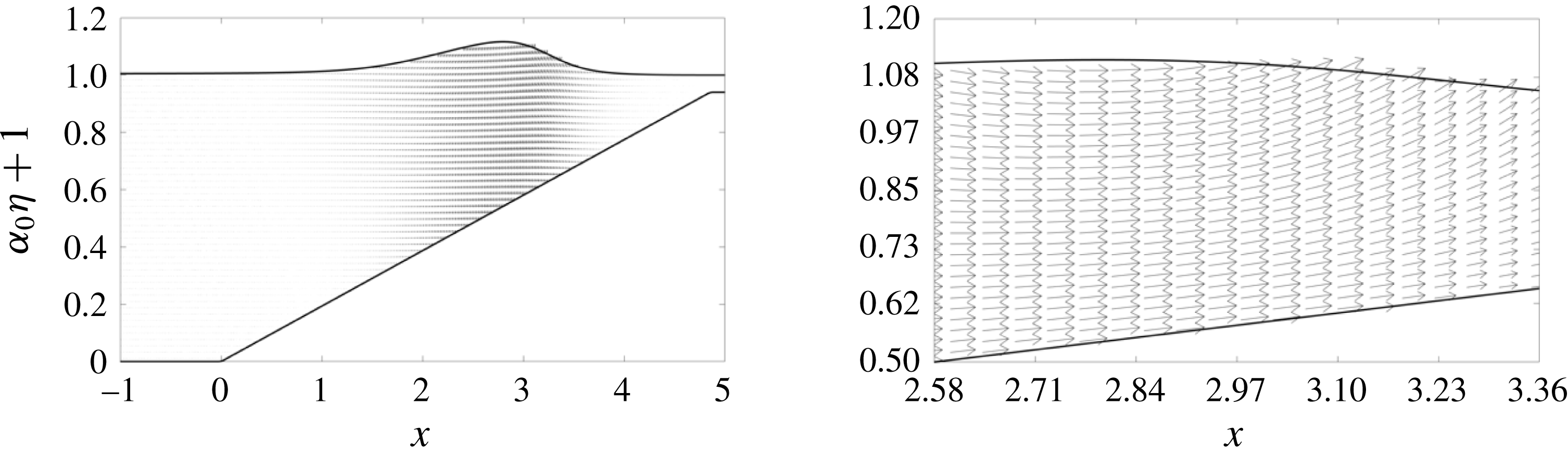
Figure 7 shows the computed velocity field for the case with
 $\unicode[STIX]{x1D6FC}_{0}=0.1$
and
 $\tan \unicode[STIX]{x1D703}=1/20$
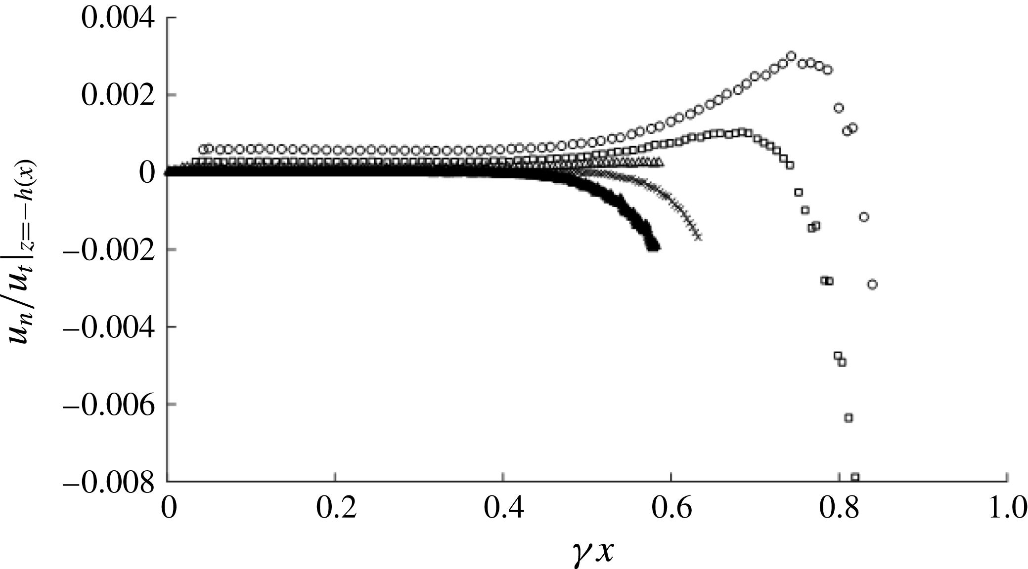
. The velocity field appears to obey the physical pattern of a shoaling wave. In order to confirm that the algorithm satisfies the bottom boundary condition (5.9), the no-flux condition along the beach bed is quantitatively evaluated by monitoring the ratio of the normal to the tangential velocities,
 $u_{n}/u_{t}$
, at the moment of time when the maximum tangential velocity occurs. The results are presented in figure 8 for the conditions of
 $\unicode[STIX]{x1D6FC}_{0}=0.1$
with
 $\tan \unicode[STIX]{x1D703}=1/12$
,
 $1/15.4$
,
 $1/21.6$
,
 $1/36$
and
 $1/100$
. The errors shown in the figure are practically nil up to the midpoint of the beach (
 $\unicode[STIX]{x1D6FE}x=\tilde{x}/L_{b}=0.5$
) prior to the commencement of wave breaking. Even at the final stage of wave breaking, the maximum error remains less than 0.4 %. The errors are associated with the perturbation and Taylor expansions in (5.10). Consequently, figure 8 shows that the present pseudo-spectral model is capable of simulating the no-flux flow condition on plane beaches accurately.
Velocity field of the shoaling solitary wave for
 $\unicode[STIX]{x1D6FC}_{0}=0.1$
and
 $\tan \unicode[STIX]{x1D703}=1/20$
. The velocity vectors shown by the arrows are not scaled.

Ratio of the velocity components normal (
 $u_{n}$
) and tangential (
 $u_{t}$
) to the beach surface for the initial wave amplitude
 $\unicode[STIX]{x1D6FC}_{0}=0.1$
with the beach slopes
 $\tan \unicode[STIX]{x1D703}=1/12$
(○),
 $1/15.4$
(▫),
 $1/21.6$
(▵),
 $1/36$
(
 $\times$
) and
 $1/100$
(▴). The maximum error occurs during the wave breaking process.

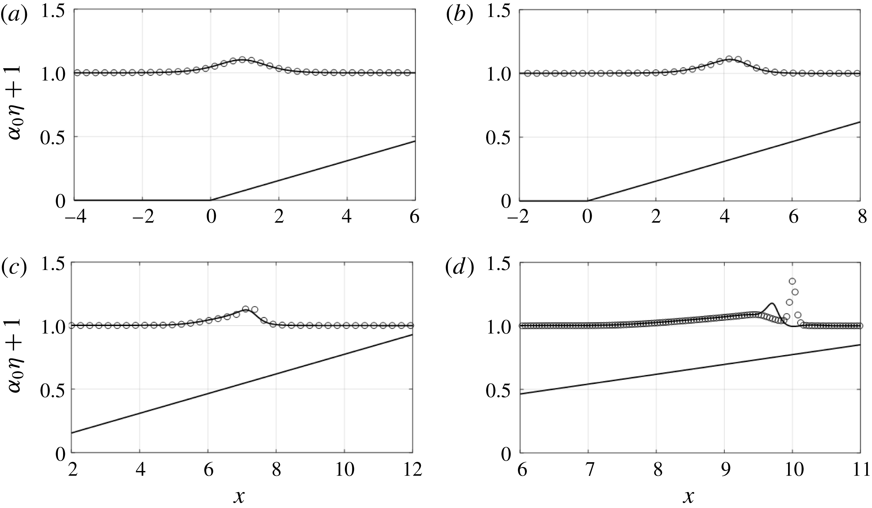
Figure 9 compares the wave profiles predicted by the vKdV theory and the pseudo-spectral Euler model. (Note that the results of the vKdV theory are numerically computed from (4.1).) A good agreement is observed until the wave becomes steepened and skewed due to the final stage of the shoaling process towards wave breaking. Then, the wave crest of the vKdV theory moves faster than the Euler model, departing from the trailing long-wave lump. It is noted that such a trend – the wave crest of the vKdV prediction advances faster than the Euler model prediction – is also observed for other cases with different beach slopes: for brevity, the results are not shown here.
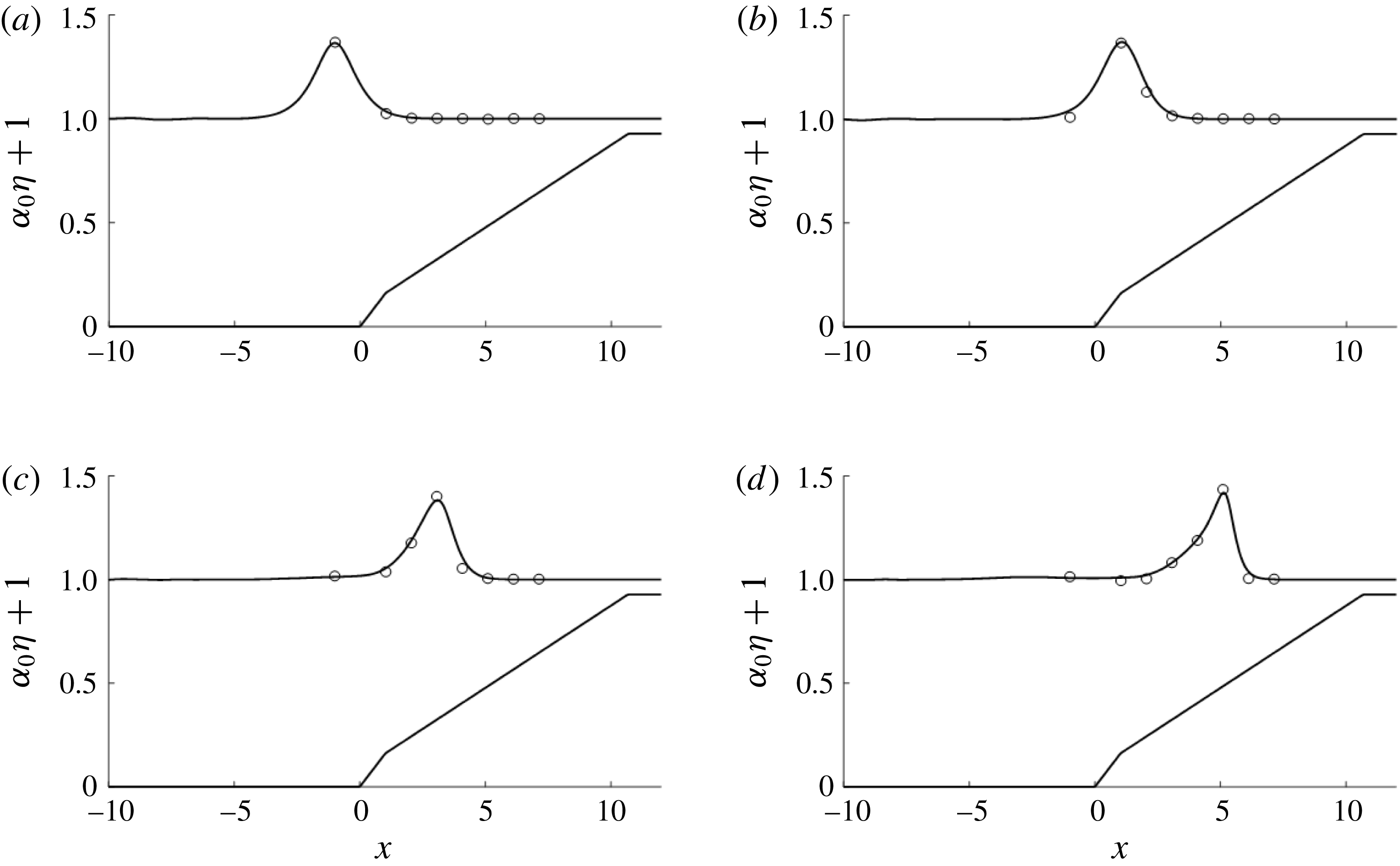
The validity of the present model is confirmed by comparing the computed results with data from the laboratory experiments. Figure 10 shows good agreement between numerical predictions and the measured laboratory data obtained in the large-scale flume. The laboratory wave flume is 110 m long, 3.7 m wide and 4.6 m deep, capable of generating clean solitary waves with a piston-type wavemaker system having a maximum stroke length of 4 m and a maximum speed of
 $4~\text{m}~\text{s}^{-1}$
. Ten discrete concrete slabs (3.7 m long and 3.7 m wide) are used to construct the beach in the wave flume, consisting of a constant depth adjacent to a composite beach of the slope
 $\tan \unicode[STIX]{x1D703}=1/12$
for the first slab at the beach toe, followed by a series of slabs laying on a slope of
 $\tan \unicode[STIX]{x1D703}=1/24$
. The beach toe (
 $x=0$
) is located at 21.3 m from the wave paddle, and the beach length from the toe is 32.9 m to the flat plateau at an elevation 1.753 m from the flume bed. Detailed descriptions of the laboratory apparatus and procedures can be found in Ko & Yeh (Reference Ko and Yeh2018). The data presented in figure 10 are obtained with the conditions of
 $h_{0}=1.888~\text{m}$
, and the incident solitary-wave amplitudes,
 $a_{0}=0.755~\text{m}$
. The agreement of the numerical results with the laboratory data is very good. Although not shown for brevity, predictions by the present numerical model are also compared and found to be in very good agreement with the data obtained from the small-scale laboratory apparatus by Grilli et al. (Reference Grilli, Subramanya, Svendsen and Veeramony1994), as well as the data of the variations of shoaling exponents given in figure 2.
Evolution of the water-surface profiles compared with the predictions made by the vKdV theory (4.1) (○) with the full-water-wave theory computed by the pseudo-spectral method (solid line), for
 $\unicode[STIX]{x1D6FC}_{0}=0.1$
and
 $\tan \unicode[STIX]{x1D703}=1/50$
: (a)
 $t=13.8$
, (b)
 $t=17.3$
, (c)
 $t=20.7$
, (d)
 $t=24.2$
.

Comparisons of numerical predictions (solid line) with the laboratory experiments (open circles). The large-scale experiments on a composite beach starting at
 $\tan \unicode[STIX]{x1D703}_{1}=1/12$
for 3.66 m, leading to
 $\tan \unicode[STIX]{x1D703}_{2}=1/24$
: the beach toe is located at
 $x=0$
and the wave crest originates 21.39 m to the left of the beach toe. Here
 $a_{0}=0.755~\text{m}$
,
 $h_{0}=1.888~\text{m}$
: (a)
 $t=4.39$
, (b)
 $t=6.25$
, (c)
 $t=8.04$
, (d)
 $t=9.65$
.

6 Results
With confidence built by the model validations and verifications in § 5.2, we now apply our numerical model to a variety of shoaling cases that are appropriate for laboratory and field conditions. We study the shoaling of solitary waves for the following range of incident values of nonlinearity
 $\unicode[STIX]{x1D6FC}_{0}=0.003{-}0.2$
and a variety of plane beach slopes, ranging from
 $\tan \unicode[STIX]{x1D703}=1/10$
to
 $\tan \unicode[STIX]{x1D703}=1/400$
in consideration of typical conditions on the Earth. As discussed earlier, the shoaling of solitary waves obeys Green’s law (
 $a\propto h^{r}$
,
 $r=-1/4$
) in the offshore part of the beach (near the beach toe) when the wave amplitude is small (Shuto Reference Shuto1973; Synolakis Reference Synolakis1990). According to Shuto (Reference Shuto1973) and Synolakis & Skjelbreia (Reference Synolakis and Skjelbreia1993), the shoaling amplification rate increases as the waves approach the shore:
 $a\propto h^{r}$
,
 $r\rightarrow -1$
. (This shoaling amplification rate is equivalent to that of the adiabatic process.) On the other hand, the recent laboratory observations as shown in figure 2 by Pujara et al. (Reference Pujara, Liu and Yeh2015) suggest that the shoaling amplification for solitary waves with
 $\unicode[STIX]{x1D6FC}_{0}>0.1$
is slower than Green’s law and approaches
 $r\approx -1/10$
, while the shoaling obeys Green’s law when
 $\unicode[STIX]{x1D6FC}_{0}\ll 0.1$
. The observed slower shoaling rate
 $|r|<1/4$
for a finite-amplitude solitary wave supports the prediction of the vKdV theory presented in § 4. We also discussed in § 3 that the shoaling evolution is limited by the wave propagation distance along the sloping beach; the beach length depends on the slope and is always finite. We then conjecture that the beach length scale
 $L_{b}$
in (3.3) and the wave length scale
 $L_{0}$
in (3.2) must be important parameters to characterize the shoaling process of solitary waves.
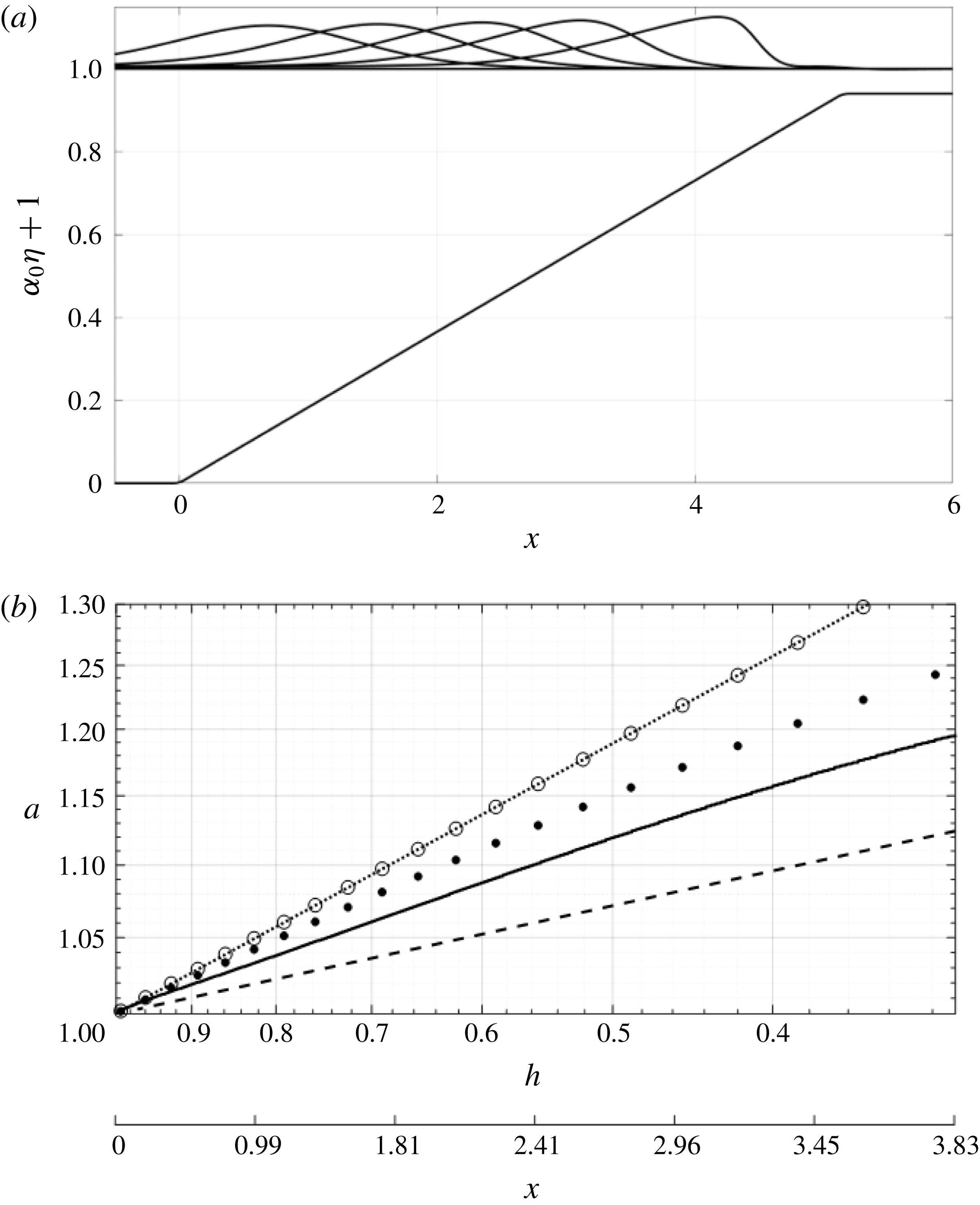
Computed shoaling process for
 $\unicode[STIX]{x1D6FC}_{0}=0.1$
and the beach slope
 $\tan \unicode[STIX]{x1D703}=1/20$
. (a) The wave-profile evolution. (b) The shoaling-wave amplification plotted in the log–log scale: solid line, present numerical prediction; dotted line, Green’s law; dashed line, the power exponent
 $r=-1/10$
; ○, linear dispersive prediction (4.9); ●, nonlinear non-dispersive prediction (4.13).

6.1 Shoaling behaviours
Figure 11(a) shows the evolution of the water-surface profile with an offshore amplitude of
 $\unicode[STIX]{x1D6FC}_{0}=0.1$
with a beach slope of
 $\tan \unicode[STIX]{x1D703}=1/20$
. The wave amplitude increases due to shoaling and the waveform becomes skewed to form a pitched-forward shape before breaking: it is the typical wave shoaling pattern described for wind waves on a mild-slope beach (see e.g. Flick, Guza & Inman Reference Flick, Guza and Inman1981; Elgar, Freilich & Guza Reference Elgar, Freilich and Guza1990). The increase in wave amplitude during the shoaling process is shown in figure 11(b). The rate of increase is slower than that of Green’s law, but faster than the rate proportional to
 $a\propto h^{-1/10}$
(this rate is shown in figure 2 for a large value of
 $\unicode[STIX]{x1D6FC}_{0}$
and presented in figure 11
b as a reference). Also plotted in figure 11(b) are the vKdV predictions for linear dispersive waves (4.9) and nonlinear non-dispersive waves (4.13). The numerical prediction shows a slower growth rate in amplitude than the predictions made by both approximations of the vKdV equation. Also note that the vKdV solution for linear dispersive waves is practically the same as that of Green’s law – as we discussed in figure 4, the dispersion effect is insensitive for a small beach slope
 $\tan \unicode[STIX]{x1D703}$
. It is important to note that the numerical prediction in figure 11(b) indicates that the amplitude growth does not follow a power law: the prediction plotted in the log–log scale is not linear, and the rate of shoaling decreases as the wave approaches the shore. Note that, for this case, the wave length scale is comparable to the beach length scale:
 $\unicode[STIX]{x1D6FE}=L_{0}/L_{b}\approx 0.2$
(see (3.4)).
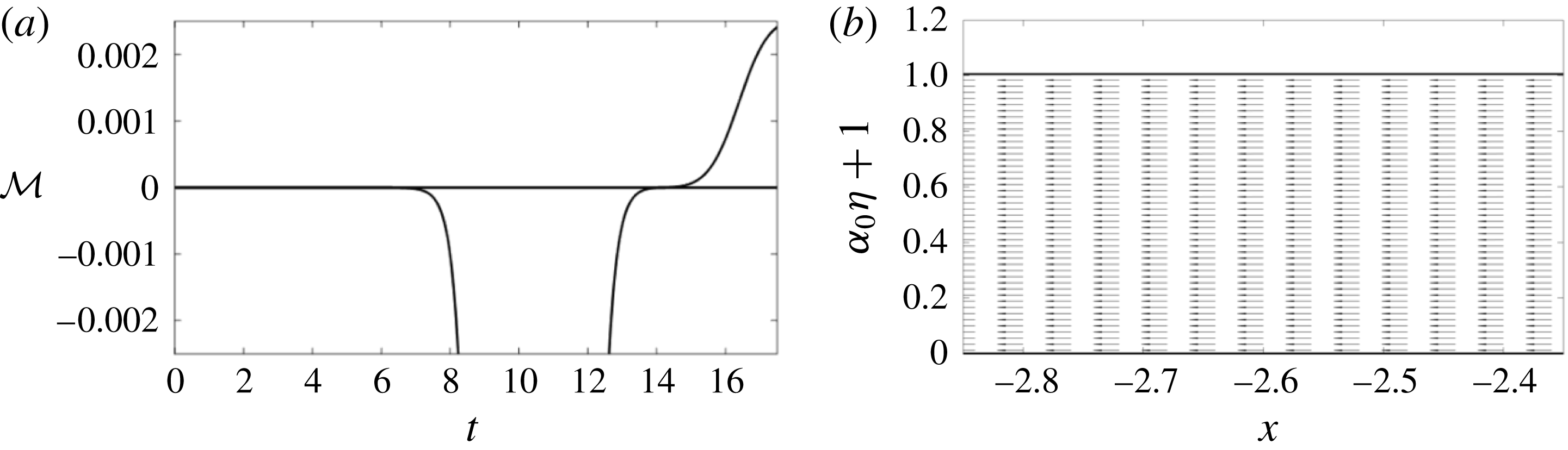
The numerical result reveals that the beach with the slope
 $\tan \unicode[STIX]{x1D703}=1/20$
causes wave energy reflection. Figure 12 shows the momentum flux
 $$\begin{eqnarray}{\mathcal{M}}=\int _{-1}^{\unicode[STIX]{x1D6FC}_{0}\unicode[STIX]{x1D702}}(\unicode[STIX]{x1D6F7}_{x})^{2}\,\text{d}z\end{eqnarray}$$
at
 $x=-2.58$
and the velocity field at
 $t=16.0$
. The momentum flux towards offshore at the end of the computation is small but finite: approximately 0.28 % of the maximum incident momentum flux. The flow speed of the outgoing wave shown in figure 12(b) is 3.2 % of the maximum flow speed of the incident solitary wave. Though small, wave reflection from the beach is evident, indicating a small leakage of offshore wave energy during the shoaling process.
Evidence of wave reflection from the beach. (a) Temporal variation of the linear momentum flux
 ${\mathcal{M}}$
given in (6.1) at
 $x=-2.58$
. The momentum flux at
 $t=17.97$
is approximately 0.28 % of the maximum incident momentum flux that occurred at
 $t=10.41$
. For convenience, we express the positive flux in the offshore direction, and negative flux represents the onshore direction. (b) The velocity field at
 $t=16.0$
that is 3.2 % of the maximum velocity of the incident solitary wave; the offshore flow is established due to the wave reflection.

A similar analysis is made for different cases: figure 13(a) shows the evolution of the water-surface profile of the solitary wave with the amplitude
 $\unicode[STIX]{x1D6FC}_{0}=0.1$
and a very mild beach slope
 $\tan \unicode[STIX]{x1D703}=1/400$
. Note that this case represents
 $\unicode[STIX]{x1D6FE}=L_{0}/L_{b}\approx 0.009\ll \mathit{O}(1)$
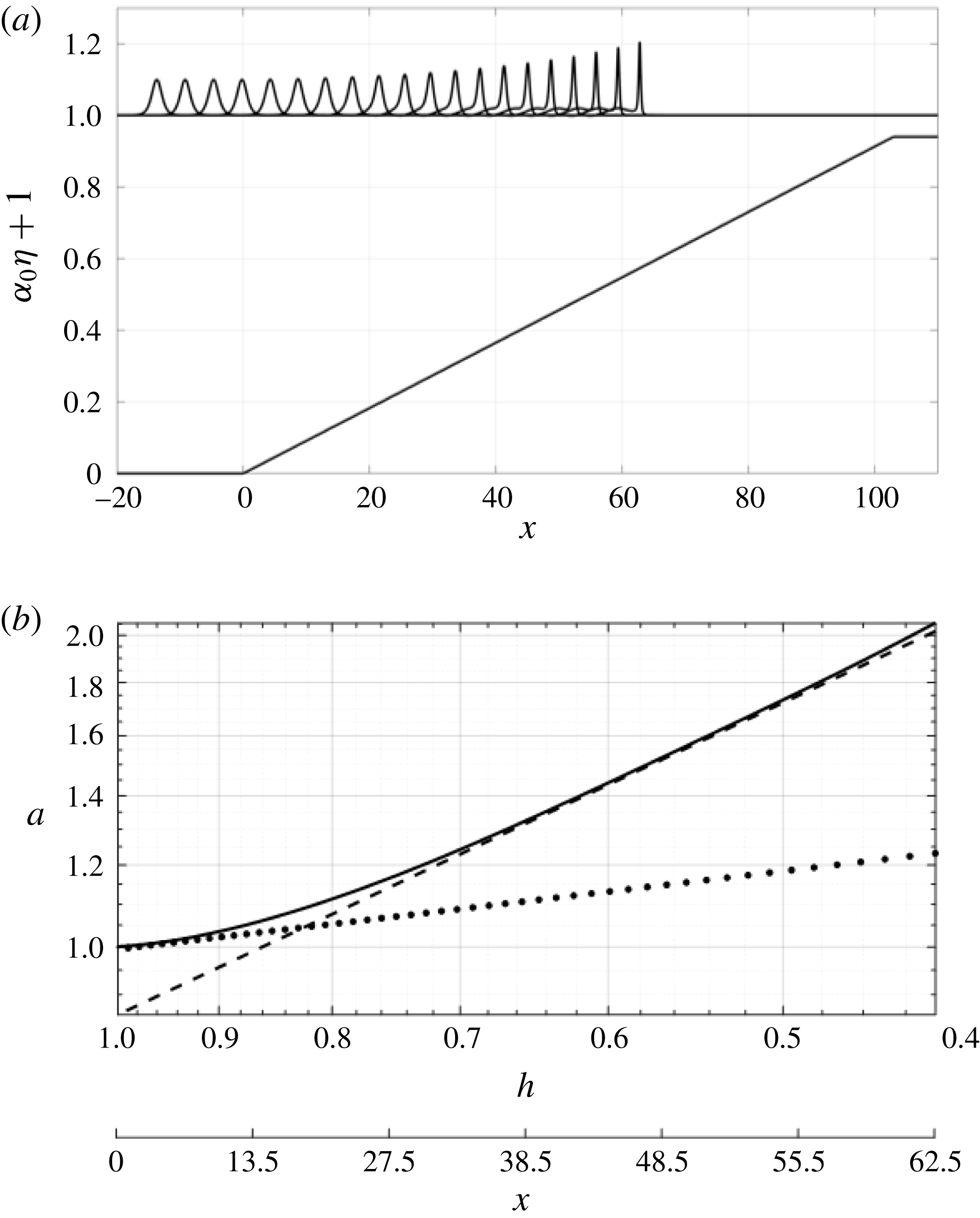
(see (3.4)), meaning that the wave length scale is much shorter than the beach length scale. Hence the incoming solitary wave is allowed to evolve over a long distance. It appears that the wave amplitude increases rapidly. The rate of increase in wave amplitude shown in figure 13(b) exhibits the shoaling predicted by the adiabatic process, i.e.
 $a\propto h^{-1}$
. It is difficult, however, to claim that the initial shoaling process obeys Green’s law
 $a\propto h^{-1/4}$
to support the ‘two-zone’ shoaling process proposed by Shuto (Reference Shuto1973) and Synolakis & Skjelbreia (Reference Synolakis and Skjelbreia1993): only the very narrow portion near the beach toe might be called Green’s law shoaling.
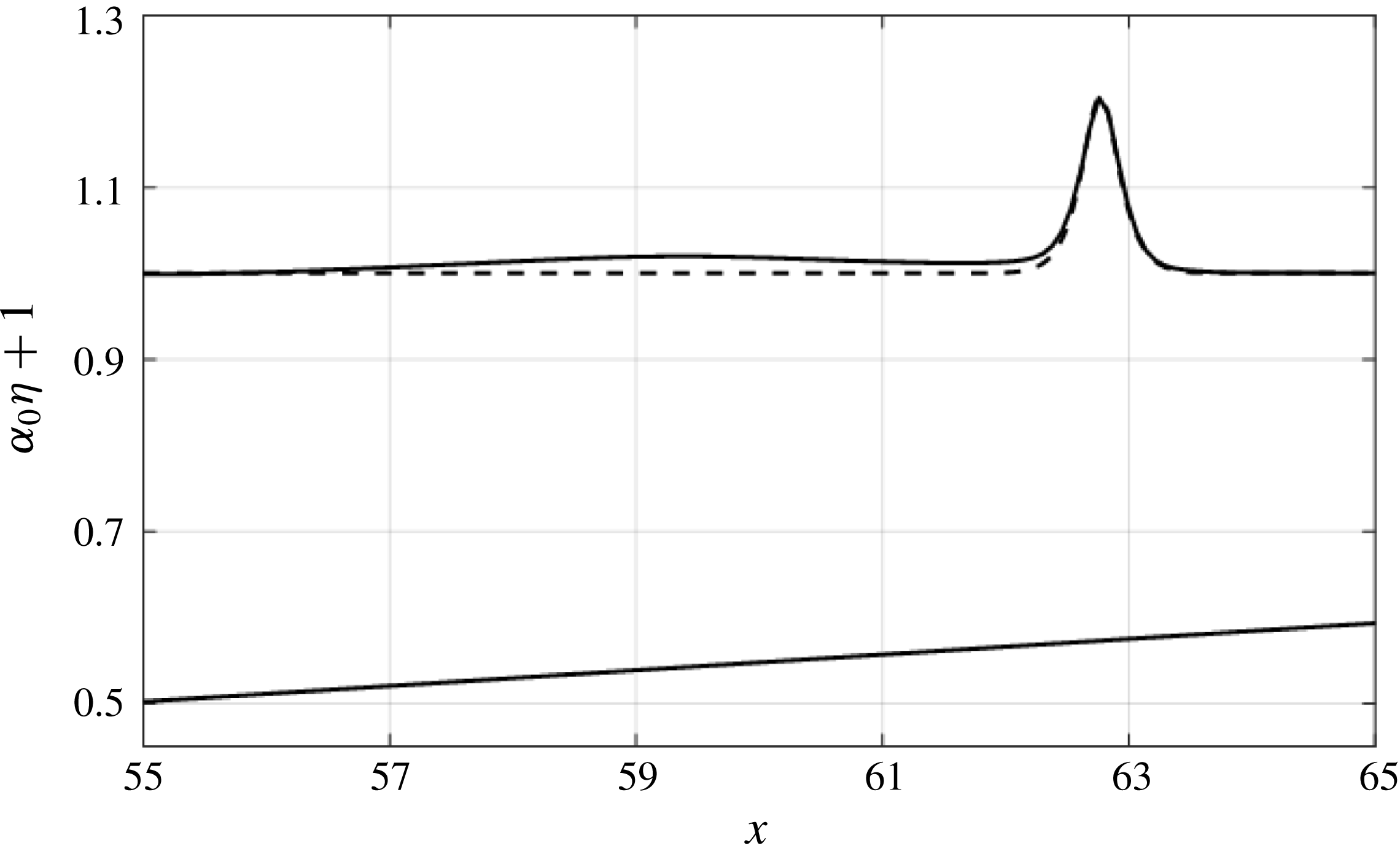
A careful observation of the wave profiles in figure 13(a) reveals the formation of a trailing long wave. Figure 14 shows the detailed wave profile together with the theoretical profile of the higher-order solitary wave given in (5.13) by Grimshaw (Reference Grimshaw1981). The figure demonstrates that the shoaling wave is indeed a solitary wave, and the shoaling exponent rate is
 $a\propto h^{-1}$
, i.e. the adiabatic process. It is also observed that the trailing wave is very long, but is not in the form of a solitary wave. Instead, it is a linear long wave. The formation of the trailing long wave is in agreement with Miles’ (Reference Miles1979) prediction to satisfy the mass conservation for the adiabatic shoaling process of a solitary wave.
Computed shoaling process for
 $\unicode[STIX]{x1D6FC}_{0}=0.1$
and the beach slope
 $\tan \unicode[STIX]{x1D703}=1/400$
. (a) The wave-profile evolution. (b) The shoaling-wave amplification plotted in log–log scale: solid line, the numerical prediction; dashed line, the adiabatic process (Boussinesq, power exponent
 $r=-1$
); dotted line, Green’s law (power exponent
 $r=-1/4$
). The intersection between Green’s law and the Boussinesq result is at
 $x=19.4$
.

Computed water-surface profile (solid line) for
 $\unicode[STIX]{x1D6FC}_{0}=0.1$
and the beach slope
 $\tan \unicode[STIX]{x1D703}=1/400$
: dashed line, the theoretical solitary-wave profile (5.13) by Grimshaw (Reference Grimshaw1971). The profile of the leading wave matches that of a higher-order solitary wave, while the trailing long wave is not a soliton.

Figure 15 shows the other extreme condition: the evolution of the water-surface profile with the incident-wave amplitude
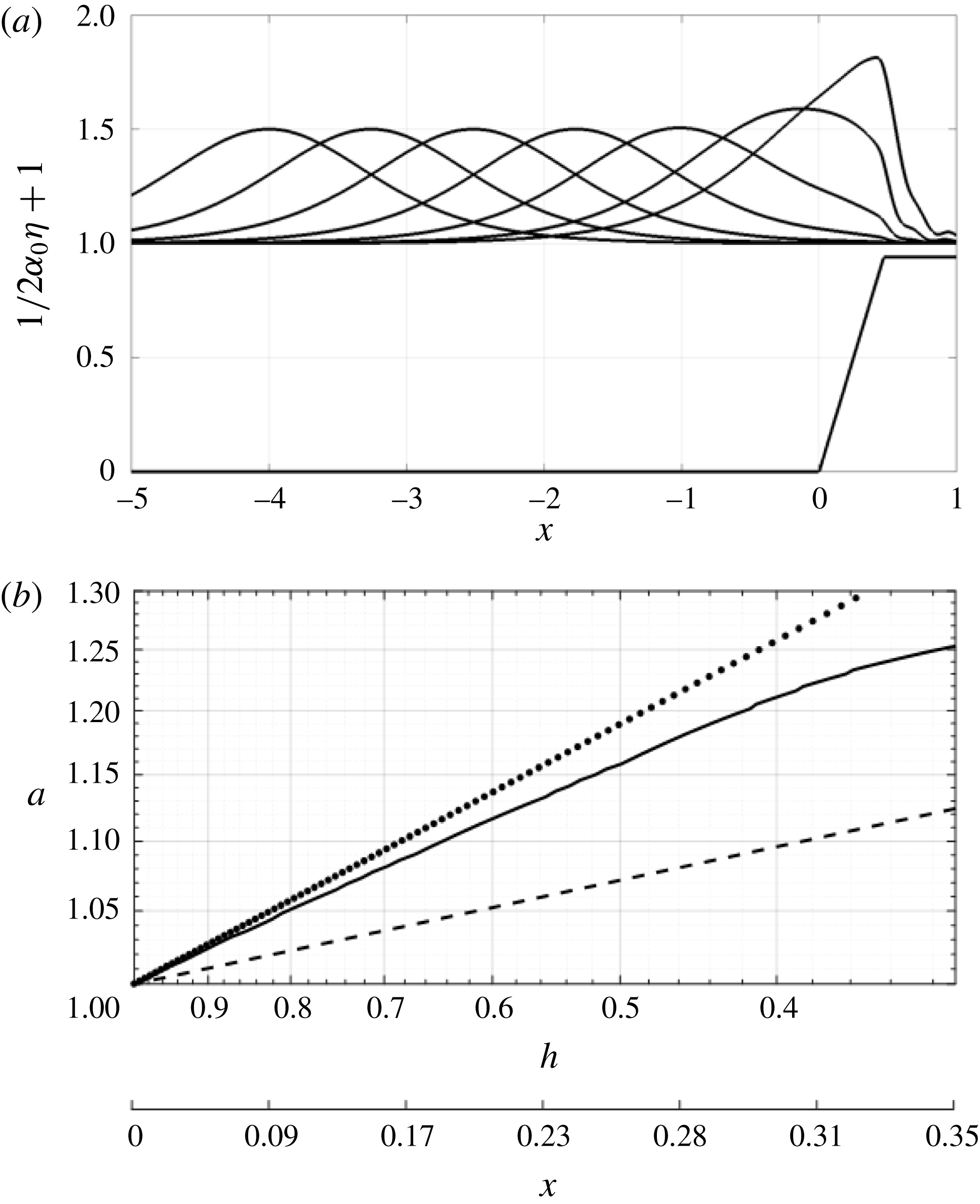
 $\unicode[STIX]{x1D6FC}_{0}=0.003$
on the steep beach with slope
 $\tan \unicode[STIX]{x1D703}=1/10$
. This case represents
 $\unicode[STIX]{x1D6FE}=L_{0}/L_{b}\approx 2$
(see (3.4)): the wave length scale is longer than the beach length scale. Figure 15(a) clearly demonstrates that only a small portion of the wave is influenced by the beach. Just like the case presented in figure 11(a), the amplitude of the solitary wave increases and the waveform becomes pitched-forward in shape, but the shoaling process is incomplete: the leading tip of the incident wave reaches the shore while the majority of the waveform remains offshore from the beach toe. Consequently, some wave energy is transmitted to the plateau of the computational domain as shown in figure 15. At the same time, the lee side of the incident wave appears to maintain its original solitary waveform. Figure 15(b) shows that the shoaling rate is slower than that of Green’s law; this is mainly due to energy leakage over the plateau in the inland direction. In addition, the wave is too long to have a chance to shoal.
6.2 On parameter
 $a^{2}h^{1/2}$

Shoaling behaviours of solitary waves are presented in terms of the parameter
 $a^{2}h^{1/2}$
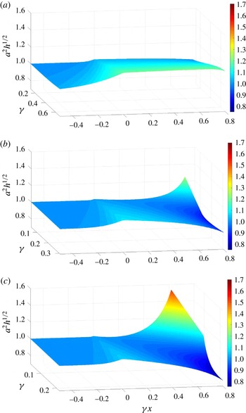
: this parameter represents the energy flux of linear non-dispersive long waves. The parameter is constant under Green’s law. Figure 16 shows the shoaling behaviours of solitary waves with the initial nonlinearity parameter
 $\unicode[STIX]{x1D6FC}_{0}=0.01$
, 0.05 and 0.1, respectively. Recall that the parameter
 $\unicode[STIX]{x1D6FE}$
defined by (3.4) expresses the ratio of the wavelength to the beach breadth; hence the smaller the value of
 $\unicode[STIX]{x1D6FE}$
, the milder the beach slope and the greater the wave amplitude. Also note that the quantity
 $\unicode[STIX]{x1D6FE}x$
represents the location: the beach toe is at
 $\unicode[STIX]{x1D6FE}x=0$
, and the shore position is at
 $\unicode[STIX]{x1D6FE}x=1.0$
. The plots in figure 16 cover approximately up to
 $\unicode[STIX]{x1D6FE}x\lessapprox 0.8$
: no calculated value is given beyond that location because of the occurrence of wave breaking.
Figure 16 indicates that the wave propagating in the region of the horizontal bed offshore amplifies as it approaches the beach toe. This beach–toe amplification effect becomes more prominent as the value of
 $\unicode[STIX]{x1D6FE}$
increases and the value of
 $\unicode[STIX]{x1D6FC}_{0}$
decreases. This offshore amplification can be attributed to the energy reflection from the beach: the steeper the beach (the larger the value of
 $\unicode[STIX]{x1D6FE}$
), the greater the reflection. Furthermore, the smaller the wave (
 $=$
the longer the wavelength), the more distance the wave front has to deform over the beach, thus enhancing the wave height even more.
In the case of
 $\unicode[STIX]{x1D6FC}_{0}=0.1$
(figure 16
c), the growth in wave amplification on the beach is slower than Green’s law, when
 $\unicode[STIX]{x1D6FE}\gtrsim 0.1$
. When
 $\unicode[STIX]{x1D6FE}\lesssim 0.1$
, the growth rate can exceed that of Green’s law, approaching the growth rate of
 $a\propto h^{-1}$
, i.e. the adiabatic evolution process: note that for this case the shoaling wave breaks early, as we discussed in figure 13. Incidentally, the results shown in figure 13 are for
 $\unicode[STIX]{x1D6FE}=0.009$
.
In the case of
 $\unicode[STIX]{x1D6FC}_{0}=0.05$
(figure 16
b), the amplification growth is also slower than that of Green’s law when
 $\unicode[STIX]{x1D6FE}$
is large, and the growth rate becomes large near the shore when
 $\unicode[STIX]{x1D6FE}$
is small (
 $\unicode[STIX]{x1D6FE}\lesssim 0.1$
). The pattern is similar to the case of
 $\unicode[STIX]{x1D6FC}_{0}=0.1$
(figure 16
c), but the deviation from the level state
 $a^{2}h^{1/2}\approx \text{const.}$
(i.e. Green’s law) is smaller in the case of
 $\unicode[STIX]{x1D6FC}_{0}=0.05$
than that of
 $\unicode[STIX]{x1D6FC}_{0}=0.1$
. In the case of
 $\unicode[STIX]{x1D6FC}_{0}=0.01$
(figure 16
a), the incident solitary wave amplifies substantially prior to the wave crest passing the beach toe: the amount of the amplification is larger when the value of
 $\unicode[STIX]{x1D6FE}$
is larger, i.e. the steeper beach slope. Then, the results show that the amplification approximately follows Green’s law thereafter:
 $a^{2}h^{1/2}\approx \text{const}$
.
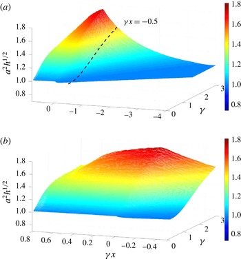
Figure 17(a) shows the similar plot of the parameter
 $a^{2}h^{1/2}$
for a very small solitary wave,
 $\unicode[STIX]{x1D6FC}_{0}=0.003$
. Figure 17(b) shows a run-up portion of figure 17(a):
 $\unicode[STIX]{x1D6FE}x>-0.5$
. In figure 17(a), the incident wave commences to amplify in the region far offshore from the beach toe because of its very long wavelength – the leading tongue of the incoming solitary wave is affected by the presence of the beach even though the crest is still travelling far offshore. In addition, when the value of
 $\unicode[STIX]{x1D6FE}$
is large, the reflection from the steep beach influences the incoming wave. Because the wavelength is so long in comparison with the (steep) beach length, wave reflection must be the primary phenomenon, rather than wave shoaling. When the value of
 $\unicode[STIX]{x1D6FE}$
is small (say
 $\unicode[STIX]{x1D6FE}\lesssim 1.0$
), the shoaling process follows Green’s law, i.e. the values of
 $a^{2}h^{1/2}$
remain constant, as shown in the figure as the horizontal trajectory on the beach
 $\unicode[STIX]{x1D6FE}x>0$
. Then, for
 $\unicode[STIX]{x1D6FE}\gtrsim 1.0$
, the rate of amplification on the beach becomes slower than that of Green’s law. This slower amplification rate can be the effect of energy leakage to the inland because of the artifact of the computational domain that we needed to set for the pseudo-spectral method.
Computed shoaling process for
 $\unicode[STIX]{x1D6FC}_{0}=0.003$
and the beach slope
 $\tan \unicode[STIX]{x1D703}=1/10$
. (a) The wave-profile evolution. (b) The shoaling-wave amplification plotted in log–log scale: solid line, the numerical prediction; dotted line, Green’s law (power exponent
 $r=-1/4$
); dashed line, power exponent
 $r=-1/10$
.

Shoaling evolution of energy flux (
 $\propto a^{2}h^{1/2}$
) along a beach:
 $\unicode[STIX]{x1D6FE}x=0$
is at the beach toe and
 $\unicode[STIX]{x1D6FE}x=1.0$
represents the shore location. The parameter
 $\unicode[STIX]{x1D6FE}=L_{0}/L_{b}$
represents the ratio of the wavelength to the beach breadth. (a)
 $\unicode[STIX]{x1D6FC}_{0}=0.01$
; (b)
 $\unicode[STIX]{x1D6FC}_{0}=0.05$
; (c)
 $\unicode[STIX]{x1D6FC}_{0}=0.10$
.

Shoaling evolution of energy flux (
 $\propto a^{2}h^{1/2}$
) for a very long incoming wave with
 $\unicode[STIX]{x1D6FC}_{0}=0.003$
:
 $\unicode[STIX]{x1D6FE}x=0$
is located at the beach toe and
 $\unicode[STIX]{x1D6FE}x=1.0$
represents the shore location. The parameter
 $\unicode[STIX]{x1D6FE}=L_{0}/L_{b}$
represents the ratio of the wavelength to the beach breadth. (a)
 $-4.0\leqslant \unicode[STIX]{x1D6FE}x\leqslant 0.8$
; (b)
 $-0.5\leqslant \unicode[STIX]{x1D6FE}x\leqslant 0.8$
, the domain left of the broken line shown in (a).

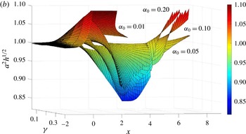
Overlays of energy flux (
 $a^{2}h^{1/2}$
) for
 $\unicode[STIX]{x1D6FC}_{0}=0.01$
, 0.05, 0.10 and 0.20. A common trend can be seen among the different layers.

7 Summary and conclusions
Shoaling processes of solitary waves are studied. A classic prediction for shoaling-wave amplification is Green’s law – wave amplitude grows proportional to
 $h^{-1/4}$
. Green’s law is for linear non-dispersive long waves under unidirectional propagation. On the other hand, the shoaling-wave amplitude is supposed to grow at a much faster rate,
 $a\propto h^{-1}$
, if the wave maintains its solitary-wave formation, i.e. the adiabatic shoaling process. Some laboratory measurements (as well as the recent tsunami measurements in the ocean) indicate, however, that the shoaling amplitude growth rate of the localized incident waves is slower than the prediction of Green’s law. It is hypothesized that the discrepancy from the existing predictions must be attributed to the factors overlooked in the theories. Obvious missing factors in Green’s law are nonlinearity and frequency-dispersion effects and wave reflection from the beach; the adiabatic shoaling process requires the incident wave to keep its solitary-wave form. Furthermore, the theory does not recognize the finiteness in beach slope and beach length. We show that the available propagation distance on the beach is an important factor: the ratio of the length scale of the solitary wave
 $L_{0}$
to the beach breadth
 $L_{b}$
, i.e.
 $\unicode[STIX]{x1D6FE}\equiv L_{0}/L_{b}$
, is crucial to characterize the shoaling processes of solitary waves.
We first analyse this problem with the use of the vKdV theory (4.1), and found that both nonlinearity and frequency-dispersion effects influence the reduction of shoaling amplification rate from Green’s law (
 $a\propto h^{-1/4}$
): the nonlinearity effect is, however, more effective in reducing the amplification growth than the frequency-dispersion effect. In fact, the effects of frequency dispersion can be considered negligible on beaches with realistic slopes, and this is explicitly demonstrated by figure 4. For example, even if the slope is steep (
 $\tan \unicode[STIX]{x1D703}=1/12$
) we find
 $a\propto h^{-0.249}$
according to (4.9), practically the same as Green’s law. This result is consistent with the previous understanding (see e.g. Yeh, Liu & Synolakis Reference Yeh, Liu and Synolakis1996; Madsen, Fuhrman & Schäffer Reference Madsen, Fuhrman and Schäffer2008; Madsen & Schäffer Reference Madsen and Schäffer2010).
The fifth-order pseudo-spectral numerical model for the full-water-wave Euler theory is used to simulate the shoaling of solitary waves. The numerical simulations can approximately realize the adiabatic evolution process (
 $a\propto h^{-1}$
) when the beach slope is very small and incident solitary-wave amplitude is large. We found that Green’s law is not the norm but is valid only for small incident-wave amplitudes and relatively small values of
 $\unicode[STIX]{x1D6FE}\lesssim 1.0$
. We conjecture that this discrepancy must be attributed to nonlinear effects during the shoaling process – for example, a trend to become a forward tilting skewed wave formation. The following behaviours of solitary-wave shoaling are observed.
(i) An incoming solitary wave amplifies prior to its crest reaching the beach toe. This amplification becomes larger when the wavelength of the incoming solitary wave is longer (i.e. small
$\unicode[STIX]{x1D6FC}_{0}$
), and the beach slope is steeper (i.e. large
$\unicode[STIX]{x1D6FE}$
). This must be due to the wave reflection caused at the beach toe and the surface.(ii) Green’s law (
$a\propto h^{-1/4}$
) can predict the shoaling of a solitary wave when its nonlinearity parameter
$\unicode[STIX]{x1D6FC}_{0}$
is small (
${\lesssim}0.01$
) and the beach slope is small: the parameter
$\unicode[STIX]{x1D6FE}=L_{0}/L_{b}$
is smaller than
$\mathit{O}(1)$
.(iii) Our analysis of the vKdV theory demonstrated that the shoaling amplification rate is slower than Green’s law when the nonlinearity effect alone is ignored. The same is the result when the dispersion effect alone is eliminated. On the other hand, it is interesting to point out that the much faster amplification rate of the adiabatic evolution (
$a\propto h^{-1}$
) is supported by a combination of nonlinear and dispersion effects.(iv) Adiabatic shoaling evolution (
$a\propto h^{-1}$
) is realizable when the nonlinearity parameter is large
$\unicode[STIX]{x1D6FC}_{0}\gtrsim 0.1$
and the beach slope is very small, i.e. the beach-slope parameter
$\unicode[STIX]{x1D6FE}$
must be very small (
$\unicode[STIX]{x1D6FE}=L_{0}/L_{b}\lesssim \mathit{O}(0.01)$
). It should be noted that, although it is not impossible, this condition to support realizing adiabatic shoaling is very limited. Note that the simulated shoaling process reveals the creation of a very long and small-amplitude wave trailing the solitary wave under the adiabatic shoaling evolution.(v) Shoaling of a solitary wave takes place at a slower rate (
$a\propto h^{-r}$
,
$r<1/4$
) than Green’s law, when the nonlinearity parameter is finite
$\unicode[STIX]{x1D6FC}_{0}\approx \mathit{O}(0.1)$
and the beach slope parameter
$\unicode[STIX]{x1D6FE}=L_{0}/L_{b}$
is also small
${\approx}\mathit{O}(0.1)$
. Note that this range of parameters coincides with the vKdV limit.(vi) In general, the rate of shoaling appears to change during the shoaling process and does not appear to follow a power law during any stage of its evolution. From these results, it may also be concluded that the linear long-wave theory cannot yield accurate predictions for shoaling processes: this is because the shoaling process itself unavoidably causes the enhancement of nonlinear effects as the wave approaches the shore.
(vii) There must be some factors other than the beach-slope parameter
$\unicode[STIX]{x1D6FE}=L_{0}/L_{b}$
that characterize shoaling. Figure 18 shows the overlay of figures 16(a–c) for
$\unicode[STIX]{x1D6FC}_{0}=0.01$
, 0.05 and 0.10, respectively, in addition to the case of
$\unicode[STIX]{x1D6FC}_{0}=0.20$
. We plot the results with
$x$
(normalized with the wavelength), instead of
$\unicode[STIX]{x1D6FE}x$
(normalized by the beach breadth). The results in figure 18 clearly show the similar pattern of the evolution processes, but the values of
$a^{2}h^{1/2}$
do not exactly collapse to consistent values, but slightly shifted from each other. Possible causes of the discrepancies are (a) wave reflection at the beach toe, (b) energy leakage towards the inland region, and (c) development of the wave skewness.





Shoaling behaviours and characteristics of solitary waves incident onto sloping beaches were presented. Although a solitary wave is a very special form of a localized wave, the foregoing results may lead to some insights regarding the behaviour of tsunamis on continental shelves.
Acknowledgements
Drs N. Pujara and A. Abdollahi are acknowledged for their inspirational discussions on this topic.