1 Introduction
The Miles–Howard theorem (Howard Reference Howard1961; Miles Reference Miles1961) tells us that for inviscid, infinitesimal perturbations to steady, one-dimensional, parallel shear flows, the minimum gradient Richardson number
 $Ri_{m}$
of the flow must be less than
 $1/4$
for such ‘linear’ perturbations to grow exponentially. From this, it is often argued that oceanic measurements will always find a Richardson number greater than or equal to
 $1/4$
, otherwise turbulence will ensue (see Smyth, Nash & Moum (Reference Smyth, Nash and Moum2019), and references therein), despite the very specific restrictions on the applicability of the theorem. In this paper we will examine two aspects of these restrictions – namely, that perturbations are infinitesimal and inviscid.
With finite-amplitude perturbations, nonlinear effects can no longer be neglected. There is various evidence that for flows susceptible to Kelvin–Helmholtz instability (KHI), complex nonlinear behaviour exists when
 $Ri_{m}>1/4$
. Kaminski, Caulfield & Taylor (Reference Kaminski, Caulfield and Taylor2017) showed that perturbations which grow transiently before decaying in the linearised setting can lead to turbulent-like irreversible mixing with
 $Ri_{m}>1/4$
when nonlinearity is included. Howland, Taylor & Caulfield (Reference Howland, Taylor and Caulfield2018) showed that as
 $Ri_{m}\rightarrow 1/4$
from below, the maximum amplitude of a saturated Kelvin–Helmholtz billow does not tend to zero, but to some finite value. One possible cause of these observations is that the pitchfork bifurcation, generically expected to occur (Strogatz Reference Strogatz2014) at the critical Richardson number,
 $Ri_{c}$
, is subcritical, so that finite-amplitude states exist above
 $Ri_{c}$
. This could mean that the system is bistable (meaning there are two stable states) in a certain range of
 $Ri_{m}$
with
 $Ri_{m}>Ri_{c}$
. (Note that by ‘subcritical’ here we mean those regions where the base flow is linearly stable, above
 $Ri_{c}$
, consistent with normal dynamical systems terminology, as opposed to the occasional oceanographic usage meaning below
 $Ri_{c}$
.)
Historically, the best way to determine the nature of the bifurcation has been to consider the next-order nonlinear effects – a so-called weakly nonlinear analysis. Such analysis has been performed for both of the models of a stratified shear layer we consider using critical layer theory (Maslowe Reference Maslowe1977; Brown, Rosen & Maslowe Reference Brown, Rosen and Maslowe1981; Churilov & Shukhman Reference Churilov and Shukhman1987), in some cases finding subcriticality. These results have also been confirmed, in the case of the Drazin model, using direct numerical simulations to investigate the nonlinear behaviour near criticality (Lott & Teitelbaum Reference Lott and Teitelbaum1992; Mkhinini, Dubos & Drobinski Reference Mkhinini, Dubos and Drobinski2013). However, our results suggest that the weakly nonlinear analysis can potentially be misleading, as discussed in § 4, since higher-order effects can quickly dominate. Critical layer theory has also been used to demonstrate the existence of nonlinear neutral modes in stratified shear flow, resembling Kelvin–Helmholtz billows, but with non-zero phase speed (Maslowe Reference Maslowe1973). It is inferred that such modes may exist when
 $Ri_{m}>1/4$
.
More recently, as it has become possible computationally to solve the Navier–Stokes equations directly, finding the finite-amplitude states which arise from bifurcations has emerged as an alternative. Newton’s method can be used to find solutions of nonlinear problems, such as steady states, iteratively. The introduction of Newton–Krylov methods (Edwards et al. Reference Edwards, Tuckerman, Friesner and Sorensen1994), where a Krylov-subspace method such as generalised minimal residuals (GMRES) (Saad & Schultz Reference Saad and Schultz1986) is used to solve the linear system inexactly at each Newton step, has allowed this to be applied to systems of very high dimensionality for which it is prohibitively expensive to work with the Jacobian matrices of the flow directly (for a comprehensive review, see Dijkstra et al. (Reference Dijkstra, Wubs, Cliffe, Doedel, Dragomirescu, Eckhardt, Gelfgat, Hazel, Lucarini and Salinger2014)). It is also possible to use Newton’s method to find and track bifurcation points of high-dimensional dynamical systems (Salinger et al. Reference Salinger, Bou-Rabee, Burroughs, Pawlowski, Lehoucq, Romero and Wilkes2002; Haines, Hewitt & Hazel Reference Haines, Hewitt and Hazel2011). Net & Sánchez (Reference Net and Sánchez2015) used a matrix-free bifurcation tracking technique with a Newton–Krylov method, as employed in this paper, and further extended this to find bifurcations of periodic orbits.
In this paper, we find the exact coherent states that bifurcate from the base flow at
 $Ri_{c}$
, and track these as both
 $Ri_{m}$
and
 $Re$
vary, to build a picture of the dynamical system near
 $Ri_{m}=1/4$
, and, crucially, answer the question of whether the system can be bistable above
 $Ri_{c}$
. Two different models susceptible to KHI are considered. The first, the ‘Holmboe’ model (Holmboe Reference Holmboe1960), with a hyperbolic tangent buoyancy profile, is the standard model in this field (Hazel Reference Hazel1972; Klaassen & Peltier Reference Klaassen and Peltier1985; Smyth & Peltier Reference Smyth and Peltier1991; Mallier Reference Mallier2003). However, we demonstrate that complex behaviour arises – associated with what we believe to be a previously unreported linear instability – and dominates at long times when this model is forced onto the system at finite
 $Re$
, obscuring the KHI. We then examine an alternative ‘Drazin’ model (Drazin Reference Drazin1958), with a uniform stratification, which shares many of the features of the Holmboe model but does not exhibit this complex behaviour. Note that, with the parameters studied, both the Drazin and Holmboe models are only known to be susceptible to stationary KHI, and not the propagating ‘Holmboe wave instability’ (HWI). The paper proceeds as follows: in § 2, we describe the methodology and code used. In § 3.1, a bifurcation diagram is presented for the Holmboe model, as well as a description of the newly discovered linear instability. In § 3.2, a bifurcation diagram and a full description of the dynamics is given for the Drazin model. Section 4 gives a brief discussion of these results.
2 Methodology
We consider the Boussinesq equations in two dimensions, and study the nonlinear evolution of perturbations away from a steady parallel velocity profile
 $U(z)$
and buoyancy stratification
 $B(z)$
. Solving for the perturbation away from these constant-in-time profiles is equivalent to solving for the full system, with an artificial body force to counteract diffusion. In non-dimensional form, the equations are:
 $$\begin{eqnarray}\displaystyle & \displaystyle \unicode[STIX]{x2202}_{t}u+\left(U+u\right)\unicode[STIX]{x2202}_{x}u+w\unicode[STIX]{x2202}_{z}\left(U+u\right)=-\unicode[STIX]{x2202}_{x}p+\frac{1}{Re}\left(\unicode[STIX]{x2202}_{x}^{2}u+\unicode[STIX]{x2202}_{z}^{2}u\right), & \displaystyle\end{eqnarray}$$
 $$\begin{eqnarray}\displaystyle & \displaystyle \unicode[STIX]{x2202}_{t}w+\left(U+u\right)\unicode[STIX]{x2202}_{x}w+w\unicode[STIX]{x2202}_{z}w=-\unicode[STIX]{x2202}_{z}p+\frac{1}{Re}\left(\unicode[STIX]{x2202}_{x}^{2}w+\unicode[STIX]{x2202}_{z}^{2}w\right)+Ri_{b}b, & \displaystyle\end{eqnarray}$$
 $$\begin{eqnarray}\displaystyle & \displaystyle \unicode[STIX]{x2202}_{t}b+\left(U+u\right)\unicode[STIX]{x2202}_{x}b+w\unicode[STIX]{x2202}_{z}\left(B+b\right)=\frac{1}{PrRe}\left(\unicode[STIX]{x2202}_{x}^{2}b+\unicode[STIX]{x2202}_{z}^{2}b\right), & \displaystyle\end{eqnarray}$$
 $$\begin{eqnarray}\displaystyle & \displaystyle \unicode[STIX]{x2202}_{x}u+\unicode[STIX]{x2202}_{z}w=0. & \displaystyle\end{eqnarray}$$
Here
 $u$
is the fluid velocity in the horizontal (
 $x$
) direction, and
 $w$
is the velocity in the vertical (
 $z$
) direction. Buoyancy acts in the positive
 $z$
direction. We impose periodic boundary conditions at
 $x=0$
and
 $x=L_{x}$
, and at
 $z=\pm L_{z}$
we enforce no-penetration (
 $w=0$
), stress-free (
 $\unicode[STIX]{x2202}u/\unicode[STIX]{x2202}z=0$
), and insulating (
 $\unicode[STIX]{x2202}b/\unicode[STIX]{x2202}z=0$
) boundary conditions. Given the dimensional shear layer depth
 $2L$
, velocity difference
 $2\unicode[STIX]{x0394}U$
, density difference
 $2\unicode[STIX]{x0394}\unicode[STIX]{x1D70C}$
, typical density
 $\unicode[STIX]{x1D70C}^{\ast }$
, and diffusivities of momentum
 $\unicode[STIX]{x1D708}$
and density
 $\unicode[STIX]{x1D705}$
, the Reynolds number is defined as
 $Re=(\unicode[STIX]{x0394}UL/\unicode[STIX]{x1D708})$
, the Prandtl number
 $Pr=(\unicode[STIX]{x1D708}/\unicode[STIX]{x1D705})$
, and the bulk Richardson number
 $Ri_{b}=(g/\unicode[STIX]{x1D70C}^{\ast })(L\unicode[STIX]{x0394}\unicode[STIX]{x1D70C}/\unicode[STIX]{x0394}U^{2})$
. Throughout, we take
 $Pr=1$
for simplicity. Two different choices of
 $U$
and
 $B$
are considered in §§ 3.1 and 3.2, respectively. For both background flows studied, the minimum gradient Richardson number
 $Ri_{m}$
, as relevant to the Miles–Howard theorem, is equal to the bulk Richardson number
 $Ri_{b}$
.
2.1 Discretisation
A new solver was developed to solve the Boussinesq equations around arbitrary background flows. Time integration uses a third-order Runge–Kutta–Wray scheme, and spatial derivatives are handled pseudo-spectrally in the periodic horizontal direction, and with explicitly conservative quasi-second-order finite differences in the vertical, on a non-uniform staggered grid: the
 $n$
th of
 $N$
grid points is located at
 $$\begin{eqnarray}z=\frac{L_{z}}{3}\left[2\left(\frac{2n-N-1}{N-1}\right)^{3}+\left(\frac{2n-N-1}{N-1}\right)\right].\end{eqnarray}$$
This ensures that there are more grid points near the shear layer at the centre of the domain than at the edges. The code was validated against DIABLO (Taylor Reference Taylor2008). Further, a linearised version of the same timestepper was produced, and validated against states of very low amplitude in the full nonlinear solver. For the system studied in § 3.1, a grid is used with 256 equispaced points in the streamwise direction and 512 points in the vertical direction, with a greater density of points in the middle of the domain. For the system studied in § 3.2, 128 points are used in the streamwise direction, covering a shorter domain, and 768 vertically, in order to accurately capture behaviour at higher
 $Re$
. The results are validated by reconverging certain solutions at a higher resolution of
 $384\times 768$
in § 3.1 and
 $256\times 1024$
in § 3.2.
2.2 Steady states and bifurcation points
Formally, we may describe our dynamical system as the evolution of a state
 $X$
by a time
 $t$
through
 $$\begin{eqnarray}X(t_{0}+t)=F\left(X(t_{0}),t;Ri_{b},Re\right),\end{eqnarray}$$
where
 $Ri_{b}$
and
 $Re$
are the constant parameters at which we are considering the evolution. Finding steady states of the flow is then equivalent to finding solutions to
 $$\begin{eqnarray}F(X,T;Ri_{b},Re)-X=0\end{eqnarray}$$
for some arbitrary fixed
 $T$
. It is possible, though extremely unlikely, that this will also find a periodic orbit of period
 $T$
.
Solving (2.7) is done by using Newton-GMRES (generalised minimum residual) iteration on an initial guess. Our implementation matches that employed by Chandler & Kerswell (Reference Chandler and Kerswell2013), including the use of a trust region to make the algorithm globally convergent. The GMRES iteration at each Newton step is continued until the residual is less than
 $10^{-2}$
, and the Newton iteration is continued until its residual, the norm of the left-hand side of (2.7), is less than
 $10^{-8}$
. A suitable
 $T$
must be chosen to optimise the GMRES method. A larger
 $T$
acts to precondition the equations, since if
 $T$
is small, all states will appear to be stationary. However, if
 $T$
is too large, computation will be prohibitively expensive. For our system, we found
 $T=11$
to be a good compromise.
Through trial and error, we converge a steady billow solution, the result of a very long temporal integration of (2.1)–(2.4), at
 $Re=1000$
and
 $Ri_{b}=0.2$
, in both the flows studied in this paper. Once one state is found at these particular
 $Ri_{b}$
and
 $Re$
, we converge another very close by at a different
 $Ri_{b}$
but the same
 $Re$
. We then follow the solution branch at this
 $Re$
over a range of
 $Ri_{b}$
using pseudo-arclength continuation (Keller Reference Keller and Rabinowitz1977). We examine the stability of the branch with Arnoldi iteration, using a linearised version of the same timestepping code.
The stability analysis reveals the existence of bifurcation points, where eigenvalues of the state cross a stability boundary. To continue these bifurcation points to different
 $Re$
, we use the states found by stability analysis as an initial guess in a different iterative solver. The system we solve is similar to that implemented in the Library of Continuation Algorithms (Salinger et al.
Reference Salinger, Bou-Rabee, Burroughs, Pawlowski, Lehoucq, Romero and Wilkes2002), but we use a matrix-free method, as discussed in detail in Sánchez & Net (Reference Sánchez and Net2016). We look for solutions to
 $$\begin{eqnarray}\displaystyle & \displaystyle F(X,T;Ri_{b},Re)-X=0, & \displaystyle\end{eqnarray}$$
 $$\begin{eqnarray}\displaystyle & \displaystyle F_{X}(X,Y,T;Ri_{b},Re)-Y=0, & \displaystyle\end{eqnarray}$$
 $$\begin{eqnarray}\displaystyle & \displaystyle Y\cdot A-1=0, & \displaystyle\end{eqnarray}$$
 $X$
,
 $Y$
and
 $Ri_{b}$
to be found by the iteration, but hold
 $Re$
fixed. Here
 $F_{X}(X,Y,t;Ri_{b},Re)$
is the linearised time evolution of a state
 $Y$
about a nonlinear state
 $X$
, computed using the linearised timestepper. Equation (2.8b
) enforces that
 $Y$
is a neutral eigenmode of the Jacobian at
 $X$
. We normalise
 $Y$
using (2.8c
), with some fixed arbitrary state
 $A$
, which we take to be the initially guessed value of
 $Y$
. Once bifurcation points are found at a particular
 $Re$
, they are reconverged at higher
 $Re$
. We are particularly interested in how the
 $Ri_{b}$
value of the bifurcation point varies with
 $Re$
.
Equations (2.8) find bifurcation points with purely real neutral eigenmodes – i.e. pitchfork and saddle-node bifurcations. For Hopf bifurcations, a set of five equations is needed, including two different linearised time evolutions. These arise from the real and imaginary parts of the eigenvalue
 $\text{e}^{\text{i}\unicode[STIX]{x1D703}}$
of the time-integrated system, corresponding to the purely imaginary eigenvalue
 $\text{i}\unicode[STIX]{x1D703}/T$
of the Jacobian. The following are solved for the unknowns
 $X$
,
 $Y_{1}$
,
 $Y_{2}$
,
 $Ri_{b}$
and
 $\unicode[STIX]{x1D703}$
:
 $$\begin{eqnarray}\displaystyle & \displaystyle F(X,T;Ri_{b},Re)-X=0, & \displaystyle\end{eqnarray}$$
 $$\begin{eqnarray}\displaystyle & \displaystyle F_{X}(X,Y_{1},T;Ri_{b},Re)-\cos \unicode[STIX]{x1D703}\;Y_{1}+\sin \unicode[STIX]{x1D703}\;Y_{2}=0, & \displaystyle\end{eqnarray}$$
 $$\begin{eqnarray}\displaystyle & \displaystyle F_{X}(X,Y_{2},T;Ri_{b},Re)-\sin \unicode[STIX]{x1D703}\;Y_{1}-\cos \unicode[STIX]{x1D703}\;Y_{2}=0, & \displaystyle\end{eqnarray}$$
 $$\begin{eqnarray}\displaystyle & \displaystyle Y_{1}\cdot A-1=0, & \displaystyle\end{eqnarray}$$
 $$\begin{eqnarray}\displaystyle & \displaystyle Y_{2}\cdot A=0. & \displaystyle\end{eqnarray}$$
 $A$
taken to be the initial guess of
 $Y_{1}$
, and the second enforces that
 $Y_{2}$
not be parallel to
 $Y_{1}$
, in order that we find a Hopf bifurcation, otherwise equations (2.9) reduce to (2.8). The additional computational requirements of (2.9) mean that we are unable to track Hopf bifurcations to as high Reynolds numbers as pitchfork and saddle-node bifurcations.
3 Results
3.1 Hyperbolic tangent stratification: the Holmboe model
First we consider a background profile of
 $U=\tanh z$
,
 $B=\tanh z$
. This is a commonly used model of a mixing layer, introduced by Holmboe (Reference Holmboe1960). It has the useful property that, at infinite
 $Re$
, the linear stability analysis can be performed analytically (Miles Reference Miles1963). With this choice, we find that the minimum gradient Richardson number
 $Ri_{m}$
is equal to
 $Ri_{b}$
, and so the Miles–Howard theorem tells us that the flow is certainly stable for
 $Ri_{b}>1/4$
. We choose
 $L_{x}=4\unicode[STIX]{x03C0}$
, which is one wavelength of the most unstable mode at
 $Ri_{b}=1/4$
as
 $Re\rightarrow \infty$
, assuming a domain of infinite height vertically. For numerically expediency, we take
 $L_{z}=10$
so that in fact
 $Ri_{c}$
tends to a value slightly less than
 $1/4$
as
 $Re\rightarrow \infty$
.
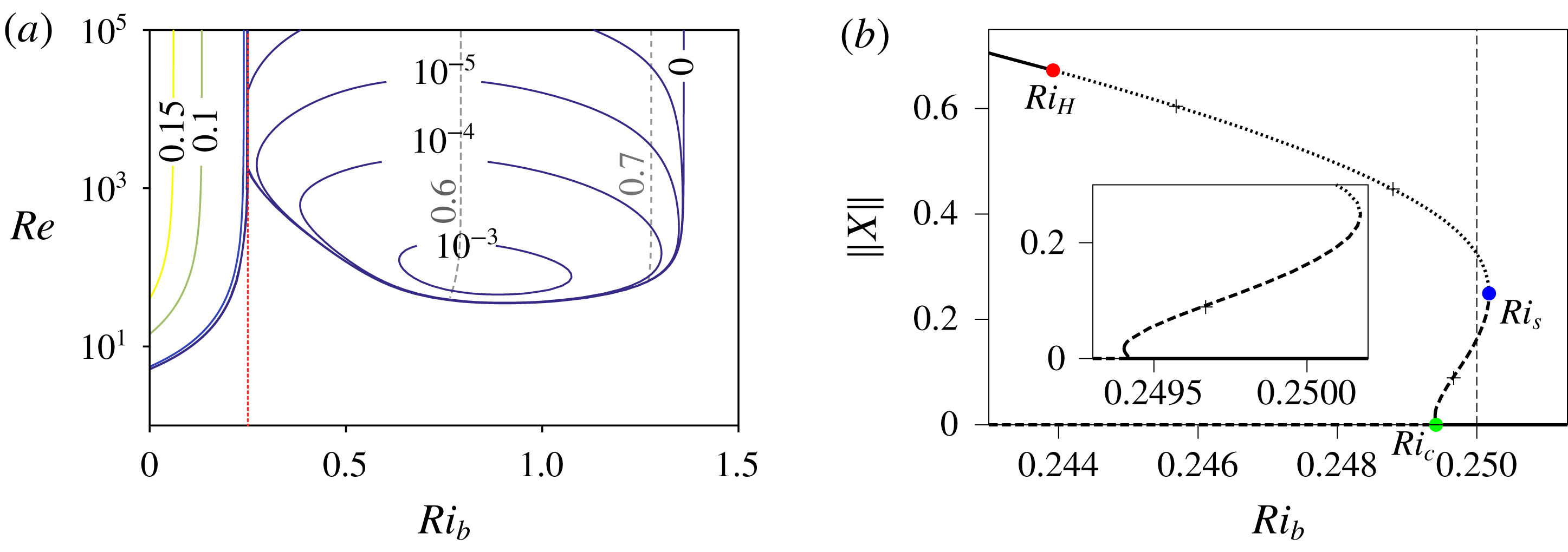
(a) Contours of the complex growth rate
 $\unicode[STIX]{x1D70E}=-\text{i}kc$
, where a normal mode is taken proportional to
 $\text{exp}\!(\!\text{i}k(x-ct)$
in a linear stability analysis of the background flow. The solid lines show the real part and the dashed grey lines show the imaginary part. For
 $Ri_{b}<1/4$
, the dominant instability mechanism is the stationary KHI, with a purely real growth rate. The newly described instability, discussed in the text, is the only one for
 $Ri_{b}>1/4$
, and has a very small growth rate, with non-zero imaginary part, and so manifests as a propagating disturbance. (b) Bifurcation diagram for the flow with hyperbolic tangent background stratification, at
 $Re=4000$
, showing the variation of
 $\Vert X\Vert$
over a (very narrow) range of
 $Ri_{b}$
. All states are unstable to the new propagating instability, but beyond that the solution branch has one further unstable eigenmode (- - - - - -), two further unstable eigenmodes (
 $\cdots \cdots$
), or is otherwise stable (——).
 $Ri_{H}$
is plotted with a red dot,
 $Ri_{s}$
with a blue dot and
 $Ri_{c}$
with a green dot. The crosses mark points converged at the higher resolution of
 $384\times 768$
.

Following Howland et al. (Reference Howland, Taylor and Caulfield2018) we define the energy of perturbations to be
 $$\begin{eqnarray}E=\frac{1}{2L_{x}}\int _{0}^{L_{x}}\text{d}x\int _{-L_{z}}^{L_{z}}\text{d}z\left(u^{2}+w^{2}+Ri_{b}b^{2}\right).\end{eqnarray}$$
State space is taken as the space of all possible incompressible perturbation flows
 $X=\left(u,w,b\right)$
, with norm
 $\Vert X\Vert :=\sqrt{2E}$
. Note that
 $p$
is not a dynamical variable as it can be calculated from a Poisson equation forced by the velocity field.
Figure 1(b) shows a bifurcation diagram at
 $Re=4000$
. Where the background state becomes unstable, with decreasing
 $Ri_{b}$
, to KHI at
 $Ri_{c}\approx 0.2494$
, a pitchfork bifurcation occurs (the green dot on figure 1
b), giving rise to a branch of finite-amplitude, billow-like states. This branch is initially stable as it bifurcates – except to the unrelated instability discussed below – and decreasing in
 $Ri_{b}$
, but there is soon a saddle-node bifurcation (see inset in figure 1
b) and it then increases in
 $Ri_{b}$
. As the unstable branch increases in amplitude,
 $Ri_{b}$
increases, and we find steady, though unstable, states above
 $Ri_{b}=1/4$
. There is another saddle-node bifurcation at
 $Ri_{s}\approx 0.250175$
(blue dot), adding a second unstable direction to the branch. (If instead we take
 $L_{z}=15$
, we find
 $Ri_{s}\approx 0.250127$
, so still
 $Ri_{s}>1/4$
.) The first saddle-node bifurcation was initially assumed to be a numerical artefact, but it was a consistent feature across all parameters studied in this model, at different resolutions. The branch stabilises at a Hopf bifurcation at
 $Ri_{H}\approx 0.244$
(red dot) when its two unstable eigenmodes simultaneously stabilise as a complex conjugate pair.
A very weak temporal linear instability, apparently hitherto unreported, is present in all states on the bifurcation diagram. As is conventional, we consider normal modes proportional to
 $\exp [\text{i}k(x-ct)]$
, where the wavenumber
 $k$
is required to be real, while the phase speed
 $c=c_{r}+\text{i}c_{i}$
is in general allowed to be complex, such that the (exponential) growth rate, generically complex, of any instability is defined to be
 $\unicode[STIX]{x1D70E}=-\text{i}kc$
. Figure 1(a) shows the maximum growth rate of linear instability of the background state, as
 $Ri_{b}$
and
 $Re$
vary. For
 $Ri_{b}>1/4$
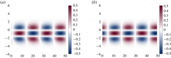
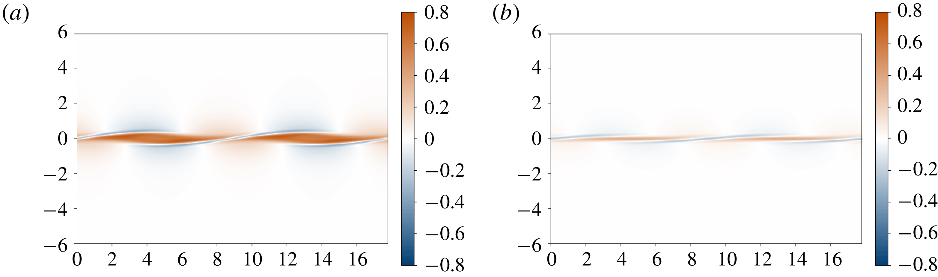
, the new instability is the dominant one. This has a phase speed of less than one, and manifests as counter-rotating rolls, advected through the domain, above and below the interface, as shown in figure 2. As
 $Re\rightarrow \infty$
, the growth rate tends to zero, as required by the Miles–Howard theorem. Close agreement of growth rates, to one part in
 $10^{3}$
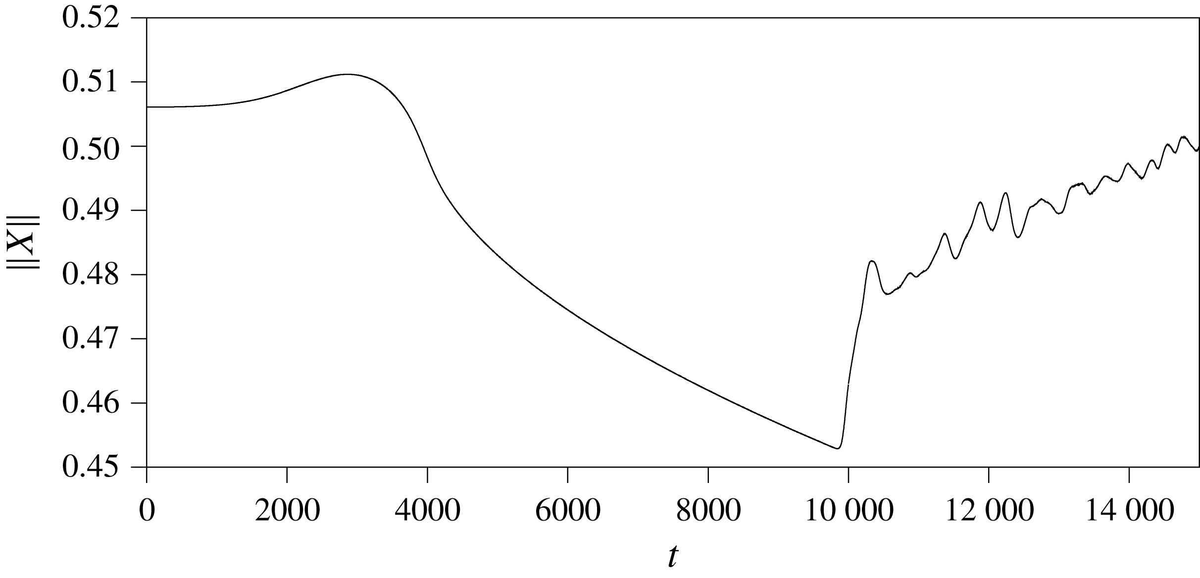
, was found for this instability between the Arnoldi stability algorithm of our code, and a direct solution of the stratified Orr–Sommerfeld equations, using a MATLAB code by W. D. Smyth (Smyth & Carpenter Reference Smyth and Carpenter2019). Despite the small growth rate, at long times this instability leads to significant nonlinear behaviour in the artificially forced problem, which eventually dominates and masks the signature of KHI. A time series of this effect is shown in figure 3. This means we are unable to give a clean description of the dynamics on a two-dimensional manifold embedded within state space, as we do for the Drazin model in the following section.
Real part of spanwise vorticity
 $\unicode[STIX]{x1D714}=\unicode[STIX]{x2202}_{x}w-\unicode[STIX]{x2202}_{z}u$
of the most unstable mode at
 $Ri_{b}=0.25$
, for a flow with (a)
 $Re=4000$
and (b)
 $Re=40\,000$
. Two domain lengths are shown horizontally. The full domain is
 $[-10,10]$
in the vertical direction. The growth rate
 $\unicode[STIX]{x1D70E}:=-\text{i}kc$
of the
 $Re=4000$
mode is
 $\unicode[STIX]{x1D70E}=3.548\times 10^{-6}+0.5229\text{i}$
. An equivalent mode also exists in the upper half of the domain, with growth rate
 $3.548\times 10^{-6}-0.5229\text{i}$
.

The perturbation amplitude along a trajectory in the Holmboe model at
 $Re=4000$
and
 $Ri_{b}=0.2478$
. The trajectory is started from a state very close to the unstable upper branch. It then follows a smooth path until approximately
 $t=10\,000$
, when the new instability has grown large enough to dominate. This then saturates and obscures the dynamics of the KHI.

3.2 Uniform stratification: the Drazin model
We now consider the case with a uniform background stratification, so that
 $U=\tanh z$
but
 $B=z$
. This is also a commonly studied problem (Drazin Reference Drazin1958; Churilov & Shukhman Reference Churilov and Shukhman1987; Thorpe, Smyth & Li Reference Thorpe, Smyth and Li2013; Kaminski, Caulfield & Taylor Reference Kaminski, Caulfield and Taylor2014) as, again, linear stability analysis can be performed analytically. As before,
 $Ri_{m}=Ri_{b}$
for this flow. Linear stability analysis on a domain of infinite height tells us we should now take
 $L_{x}=2\sqrt{2}\unicode[STIX]{x03C0}$
to achieve
 $Ri_{c}\rightarrow 1/4$
as
 $Re\rightarrow \infty$
. As before,
 $L_{z}=10$
. We use the same definition of energy
 $E$
as in the hyperbolic tangent case.
Qualitatively, the bifurcation diagram is very similar to the
 $\tanh$
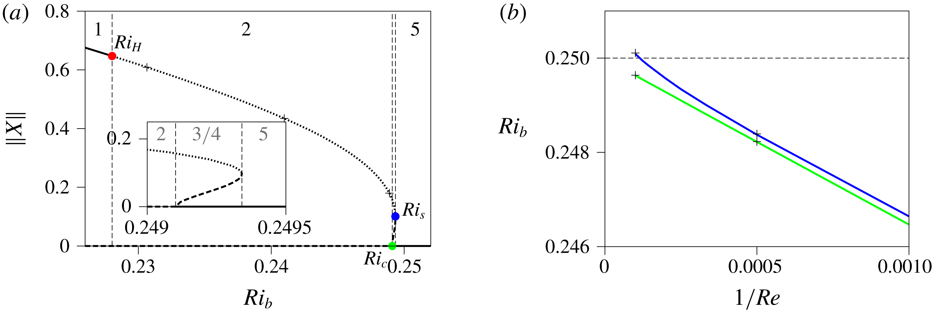
stratification case. Figure 4(a) shows the diagram for
 $Re=4000$
. The main difference from figure 1(b) is the lack of the first saddle-node bifurcation near the pitchfork. The values of the various bifurcation Richardson numbers are different; for example, the Hopf bifurcation at
 $Ri_{H}$
(shown in red) occurs at somewhat lower
 $Ri_{b}$
than before. Also crucially, the propagating linear instability described in § 3.1 is no longer present, and consequently we can study the long-time behaviour of KHI.
The period of the Hopf bifurcation at
 $Re=4000$
is approximately
 $1690$
advective time units, which is much too high to allow us to converge the resulting periodic orbit directly, but long-time integrations at a range of
 $Ri_{b}$
give us an idea of the behaviour, since it appears to be stable in this case. Even this simple method becomes useless as we approach
 $Ri_{c}$
, since the period increases towards infinity. This is the generic behaviour near a homoclinic bifurcation (Strogatz Reference Strogatz2014), which we believe occurs somewhere between
 $Ri_{c}$
and
 $Ri_{s}$
: the periodic orbit collides with the lower branch state.
(a) Bifurcation diagram of the flow with uniform background stratification, at
 $Re=4000$
. The dashed vertical lines separate the numbered regions, as discussed in the text. The solution branch has one unstable direction (- - - - - -), two unstable directions (
 $\cdots \cdots$
), or is stable (——).
 $Ri_{H}$
is plotted with a red dot,
 $Ri_{s}$
with a blue dot and
 $Ri_{c}$
with a green dot. (b) Variation of
 $Ri_{c}$
(green) and
 $Ri_{s}$
(blue) with
 $1/Re$
.
 $Ri_{s}$
passes through
 $1/4$
at
 $Re\approx 9000$
. In both figures, the crosses mark points converged at the higher resolution of
 $256\times 1024$
.

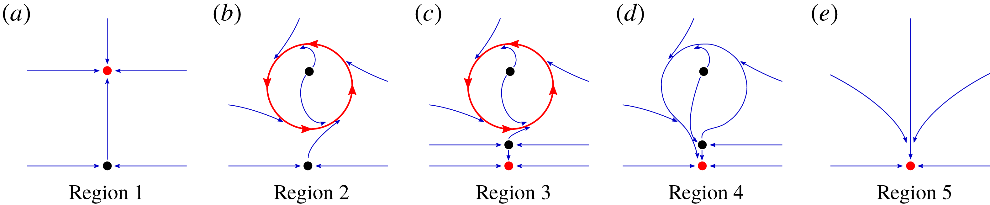
The behaviour of the system, which we believe to be generic for sufficiently high
 $Re$
, can be completely understood on a two-dimensional manifold described by the two most unstable eigenmodes; as shown schematically in figure 5. In region 1, where
 $Ri_{b}<Ri_{H}$
, the base state is unstable, and the instability saturates and eventually leads to the upper branch steady state, which is stable. For
 $Ri_{H}<Ri_{b}<Ri_{c}$
, region 2, the base state and upper branch are both unstable, and perturbations lead to a stable periodic orbit. Immediately to the right of the pitchfork bifurcation
 $Ri_{c}$
in the region 3, the base state is stable and there exists a lower branch edge state, which is unstable. If finite-amplitude perturbations to the base state are past this edge, they are attracted to the periodic orbit, and we have subcritical ‘transition’. Between regions 3 and 4, there is a homoclinic bifurcation of the periodic orbit with the lower branch state. This means that in region 4, the periodic orbit no longer exists. There are unstable finite-amplitude states and large transient trajectories, but the base state is the only attractor. In region 5, past the saddle-node bifurcation,
 $Ri_{b}>Ri_{s}$
, the base state is the only known exact coherent structure. Of course, in reality the finite-amplitude states break the translational symmetry of the base state, and there are in fact a continuum of upper branch states, periodic orbits and so on, with a shift of origin. Which of these the system is attracted to depends on the phase of the initial perturbation.
All of the stationary states we have found, as well as the periodic orbit, are the result of bifurcations away from the parallel base state. It is possible that other states exist in the system which are not connected to this base state at all; as is the case, for example, for the Nagata solutions in plane Couette flow (Nagata Reference Nagata1990). The existence of these isolated solutions would complicate the above description of the dynamical system. However, we have seen no evidence of any such states in any of our results. If they exist in our flow, therefore, we assume them to be unimportant for the range of parameters considered.
Schematics of the dynamical system restricted to the two-dimensional manifold of the two most unstable eigenmodes. The dots mark steady states, the lower being the base solution, and the lines show a few relevant trajectories. Solutions shown in red are stable, and those in black are unstable.

Figure 6 shows the vorticity structure of the steady states at two different values of
 $Ri_{b}$
. In the case of the Hopf bifurcation, billow-like structures are clearly seen, bearing a strong resemblance to the saturated, unsteady billows found by Howland et al. (Reference Howland, Taylor and Caulfield2018). Increasing
 $Ri_{b}$
along the upper branch to the saddle-node bifurcation, these structures remain but become significantly less pronounced. Baroclinic effects mean that the height of the billows decreases with increasing
 $Ri_{b}$
.
Spanwise vorticity
 $\unicode[STIX]{x1D714}=\unicode[STIX]{x2202}_{x}w-\unicode[STIX]{x2202}_{z}u$
of the stationary states at the (a) Hopf
 $Ri_{H}=0.22803$
between regions 1 and 2 and (b) saddle-node
 $Ri_{s}=0.24934$
between regions 4 and 5, for the flow in figure 4(a). Two domain lengths are shown horizontally. The full domain is
 $[-10,10]$
in the vertical direction.

We track the values of
 $Ri_{c}$
and
 $Ri_{s}$
for
 $Re$
from
 $1000$
to
 $10\,000$
using the method described in § 2.2, and the results are shown on figure 4(b). As
 $Re\rightarrow \infty$
, extrapolation, assuming linearity in
 $1/Re$
, suggests
 $Ri_{c}\rightarrow 0.25-1.4\times 10^{-5}$
, slightly less than
 $1/4$
because of the finite height of the domain. We find that
 $Ri_{s}>1/4$
for
 $Re\gtrsim 9000$
and estimate that
 $Ri_{s}\rightarrow 0.251$
as
 $Re\rightarrow \infty$
. Since we have been unable to find the location of the conjectured homoclinic bifurcation, we are unable to say whether region 3, with a stable periodic orbit, extends above
 $Ri_{b}=1/4$
, and hence whether the system is bistable here. Nevertheless, region 4 certainly exists above
 $Ri_{b}=1/4$
, so there will be nonlinear transient behaviour, with the development of Kelvin–Helmholtz style billows as shown in figure 6. We have also tracked the Hopf bifurcation (omitted from figure 4(b) for scale reasons) and this shows a similar trend to the saddle-node bifurcation.
4 Discussion and conclusions
The Miles–Howard theorem is an important result in the theory of linear stability of inviscid flows. However, the fact it seems to work in more general conditions than those for which it is proven means it has been informally applied as a ‘rule of thumb’ at high
 $Re$
. We have shown that subcritical instability can exist in such flows, so that complex nonlinear behaviour can occur even when the flow is linearly stable. This is not a new result; Maslowe (Reference Maslowe1977) found subcritical instability in the Holmboe model with
 $Pr=0.72$
and
 $Re=100$
using a weakly nonlinear analysis. We note, however, that this technique of finding the first-order correction to the linear theory would have given misleading results applied to the parameters we study, since in the Holmboe model, we find a saddle-node bifurcation very close to the pitchfork, leading to subcritical instability instead of the apparent supercriticality. Furthermore, the technique presented in this paper allows us to precisely find the location of the saddle-node bifurcations, and demonstrate explicitly that finite-amplitude billows exist at
 $Ri_{b}>1/4$
, which has only been inferred previously (Kaminski et al.
Reference Kaminski, Caulfield and Taylor2017; Howland et al.
Reference Howland, Taylor and Caulfield2018).
We have been able to give a simple description of the dynamics in the Drazin model. It is not immediately clear that the dynamics of the artificially forced system studied here will be relevant to those of an unforced system, which has traditionally been used as a model for geophysical flows. The incredibly long periods of the orbits born from the Hopf bifurcation discussed earlier, for example, mean that in an unforced problem, the background flow would have diffused almost entirely away before one complete cycle. Nevertheless, the instability of the unforced flows still leads to saturated states very similar to the steady solutions we have found, and the subcriticality we have demonstrated would certainly lead to non-trivial transient behaviour.
Our results alone do not invalidate the use of
 $Ri_{b}=1/4$
as a ‘rule of thumb’ for criticality. The subcriticality we have found extends only very slightly about
 $1/4$
in both cases studied. However, the results of Brown et al. (Reference Brown, Rosen and Maslowe1981) and Churilov & Shukhman (Reference Churilov and Shukhman1987), who respectively studied the Holmboe and Drazin models using weakly nonlinear analysis, show strong subcriticality when
 $Pr>1$
but supercriticality when
 $Pr<1$
, and that higher-order terms must be considered at our choice of
 $Pr=1$
. Preliminary results tracking the saddle-node bifurcation points in our work as
 $Pr$
varies seem to agree with this, so future research will concentrate on the more oceanographically relevant range
 $Pr\sim O(10)$
.
It should be noted that all our results have been performed at a fixed domain width
 $L_{x}$
, and yet the wavelength of maximum growth of KHI is known to vary with
 $Ri_{b}$
(Hazel Reference Hazel1972). Therefore, we expect our results would change at different
 $L_{x}$
, but since we have chosen the wavelength of maximum growth at criticality, and all our results are very close to
 $Ri_{c}$
, it is to be assumed that our domain size is the most relevant to a physical flow.
In addition to these finite-amplitude nonlinear states, we have found linear instability with
 $Ri_{b}>1/4$
in the Holmboe model (see figure 2), which disappears as
 $Re\rightarrow \infty$
, as required by the Miles–Howard theorem. A similar phenomenon was found by Miller & Lindzen (Reference Miller and Lindzen1988). However, their instability had large growth rates and required a carefully constructed flow. We have found an instability in a widely used model, hitherto unreported to the best of our knowledge. The new instability has a tiny growth rate at physically realistic
 $Re$
. This suggests it can be ignored in oceanic problems, but fails to entirely explain why it has not been discussed before. It is commonly assumed that finite-
 $Re$
effects are always stabilising compared to inviscid behaviour in such flows, despite demonstrations to the contrary (Defina, Lanzoni & Susin Reference Defina, Lanzoni and Susin1999). This instability demonstrates that such assumptions should be checked carefully. While it is not appropriate to classify this instability as ‘classic’ Holmboe wave instability, since HWI is an inviscid instability, we conjecture that it may be homotopically connected to Holmboe instability as parameters are varied, as it has a similar phase speed and occurs at similar values of
 $Ri_{b}$
. This is an area for future research.
Acknowledgements
Thanks are due to Professor W. D. Smyth and two anonymous reviewers, whose thoughtful and insightful comments have substantially improved this paper. J.P.P. is supported by an EPSRC DTA studentship. The research activities of C.P.C. and R.R.K. were supported by EPSRC Programme grant EP/K034529/1 entitled ‘Mathematical Underpinnings of Stratified Turbulence’. The data used to create figures 1(b), 2, 4(a) and 4(b) are available at https://doi.org/10.17863/CAM.43230. The numerical solver used in this paper is available at https://github.com/Jezz0r/Stratiflow.