1 Introduction
Steady incoming flow past a long circular cylinder at relatively low values of the Reynolds number (
 $Re$
) has been the topic of extensive studies due to its fundamental and practical significance. It is well known that the flow is governed by a single dimensionless parameter
 $Re$
, which is defined based on the approaching flow velocity
 $U$
, the cylinder diameter
 $D$
and the kinematic viscosity of the fluid
 ${\it\nu}$
. Methods of investigation have included physical model testing, direct numerical simulation (DNS) and linear (and nonlinear) stability analysis. Comprehensive reviews on investigations of flow with different methodologies can be found, for example, in Williamson (Reference Williamson1996a
,Reference Williamson
b
) and Posdziech & Grundmann (Reference Posdziech and Grundmann2001). Based on these investigations, it has been shown (e.g. Williamson Reference Williamson1996a
) that for flow past a circular cylinder the flow structure in the wake will undergo a transition sequence of (1) emergence of primary wake instability at
 $Re\sim 47$
, (2) onset of mode A instability with large-scale vortex dislocations (i.e. mode A*) at
 $Re\sim 190$
, (3) the gradual transition from mode A* to mode B over a range of
 $Re$
from 230 to 250, and (4) development of increasingly disordered mode B structure beyond
 $Re=260$
.
Many previous studies have focused on identifying the critical Reynolds number
 $Re_{cr}$
at which mode A* wake instability emerges. The
 $Re_{cr}$
values identified by some experimental studies are 150 by Roshko (Reference Roshko1954) and Tritton (Reference Tritton1959), 165 by Norberg (Reference Norberg1994), 178 by Williamson (Reference Williamson1988, Reference Williamson1989), 194 by Williamson (Reference Williamson1996b
), and 205 by Miller & Williamson (Reference Miller and Williamson1994). It was discovered that the low values of
 $Re_{cr}$
identified by early experimental studies were largely due to the ‘end effect’ (Williamson Reference Williamson1996b
). Williamson (Reference Williamson1996b
) extended the
 $Re_{cr}$
value to 194 by eliminating end effects using non-mechanical end conditions. This value is very close to the
 $Re_{cr}$
values of 188.5 (
 $\pm$
1.0), 190.2 (
 $\pm$
0.02) and 190.5 predicted through linear stability analysis by Barkley & Henderson (Reference Barkley and Henderson1996), Posdziech & Grundmann (Reference Posdziech and Grundmann2001) and Rao et al. (Reference Rao, Thompson, Leweke and Hourigan2013) respectively.
According to the experimental study by Williamson (Reference Williamson1996b
), mode B wake instability first emerges at
 $Re\sim 230$
, which is much lower than the critical
 $Re$
of 259 and 261 (
 $\pm$
0.2) for mode B instability predicted through linear stability analysis by Barkley & Henderson (Reference Barkley and Henderson1996) and Posdziech & Grundmann (Reference Posdziech and Grundmann2001) respectively. According to Henderson (Reference Henderson1997), this is because the existence of mode A* instability would destabilize mode B in the nonlinear interaction between the two modes. In contrast, the linear stability analyses by Barkley & Henderson (Reference Barkley and Henderson1996) and Posdziech & Grundmann (Reference Posdziech and Grundmann2001) were performed based on a two-dimensional (2D) base flow. Based on nonlinear stability analyses, Barkley, Tuckerman & Golubitsky (Reference Barkley, Tuckerman and Golubitsky2000) and Sheard, Thompson & Hourigan (Reference Sheard, Thompson and Hourigan2003) predicted
 $Re$
ranges for the transition from mode A* to mode B of 230–265 and 230–260 respectively, which are in good agreement with the transition range of
 $Re=230{-}250$
observed by Williamson (Reference Williamson1996a
) through experiments.
The experimental study by Williamson (Reference Williamson1996b ) has revealed that the wake transition from mode A* to mode B is a gradual process with intermittent swapping between the two modes. In this transition regime, two distinct vortex shedding frequencies corresponding to each of the two modes can be observed (Williamson Reference Williamson1996b ).
Investigations of the wake transitions of flow past a circular cylinder have also been attempted using three-dimensional (3D) DNS to account for the nonlinear behaviours of the flow. Williamson (Reference Williamson1996a
,Reference Williamson
b
) and Posdziech & Grundmann (Reference Posdziech and Grundmann2001) provided extensive reviews of DNS studies on the flow, and these will not be reviewed again in this study. In brief, two approaches have been employed to investigate the flow. One is the spectral element approach which employs Fourier expansion to model spanwise variations in pressure and velocity, on the assumption of spanwise periodicity in the flow structure. The second is based on the conventional finite volume method (FVM) and finite element method (FEM) formulations which are routinely applied to flows involving complex geometries. Henderson (Reference Henderson1997) and Braza, Faghani & Persillon (Reference Braza, Faghani and Persillon2001) confirmed the existence of natural vortex dislocations at
 $Re=220$
using a spectral element method and FVM respectively, with relatively large span lengths of more than
 $12D$
. Henderson (Reference Henderson1997) also examined the vorticity field and found mixed modes A* and B at
 $Re$
of 220 and 265. On the other hand, Behara & Mittal (Reference Behara and Mittal2010) studied the energy transfer from mode A* to mode B by analysing the power spectra of the velocity signal in the near wake, and found the transition occurred at
 $Re\sim 270$
(while only mode A* appeared at
 $Re=250$
), which was higher than the transition range of
 $Re=230{-}250$
reported by Williamson (Reference Williamson1996a
).
In light of these earlier works, the primary aim of this study is to investigate the wake transition from mode A* to mode B. This aim has been pursued because although the fundamental mechanisms of the wake transition from mode A* to mode B are well understood, the actual transition process has not been studied in great detail. Due to the rapid increase of computing power in recent years, it has become possible to use a high computational mesh resolution within a large domain size to run simulations for a sufficiently long flow time for the investigation of the fully developed flow. The rest of this paper is organized in the following manner. In § 2, the governing equations, numerical model and model validation are presented. The mode A* and mode B vortex structures are discussed in § 3.1. The gradual wake transition from mode A* to mode B and a critical condition at
 $Re=265{-}270$
are discussed in §§ 3.2 and 3.3 respectively. Finally, major conclusions are drawn in § 4.
2 Numerical model
2.1 Numerical method
Numerical simulations have been carried out with OpenFOAM (www.openfoam.org) to solve the continuity and incompressible Navier–Stokes equations:
 $$\begin{eqnarray}\displaystyle & \displaystyle \frac{\partial u_{i}}{\partial x_{i}}=0, & \displaystyle\end{eqnarray}$$
 $$\begin{eqnarray}\displaystyle & \displaystyle \frac{\partial u_{i}}{\partial t}+u_{j}\frac{\partial u_{i}}{\partial x_{j}}=-\frac{1}{{\it\rho}}\frac{\partial p}{\partial x_{i}}+{\it\nu}\frac{\partial ^{2}u_{i}}{\partial x_{j}\partial x_{j}}, & \displaystyle\end{eqnarray}$$
 $(x_{1},x_{2},x_{3})=(x,y,z)$
are the Cartesian coordinates,
 $u_{i}$
is the velocity component in the direction of
 $x_{i}$
,
 $t$
is the time and
 $p$
is the pressure. Equations (2.1) and (2.2) are solved with the FVM approach and the PISO (pressure implicit with splitting of operators) algorithm (Issa Reference Issa1986). The convection term is discretized using the fourth-order cubic scheme, while the diffusion term is discretized using a second-order linear scheme. A blended scheme consisting of the second-order Crank–Nicolson scheme and a first-order Euler implicit scheme is used to integrate the equations in time.
2.2 Boundary conditions
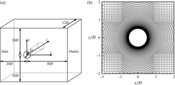
A hexahedral computational domain of
 $50D\times 40D\times 12D$
, as shown in figure 1(a), is adopted for the FVM simulations. At the inlet boundary, a uniform flow velocity
 $U$
is specified in the
 $x$
-direction. At the outlet, the Neumann boundary condition (i.e. zero normal gradient) is applied for the velocity, and the pressure is specified as a reference value of zero. A symmetry boundary condition is applied at the top and bottom boundaries, whereas a periodic boundary condition is employed at the two lateral boundaries perpendicular to the spanwise direction. A non-slip boundary condition is applied on the cylinder surface.
(a) Schematic model of the computational domain and (b) close-up view of the reference mesh near the cylinder.

2.3 Computational mesh and domain
The computational mesh and domain size have been chosen based on a thorough parameter dependence check, which is reported separately in appendix A. The selected 2D mesh and the resulting 3D mesh are referred to as the standard meshes and are used throughout the present study unless otherwise stated. The numerical results obtained with the standard meshes have been demonstrated to be generally converged and consistent with independent numerical results reported by Posdziech & Grundmann (Reference Posdziech and Grundmann2001) based on a mesh dependence check.
2.4 Model validation
The numerical model used in this study was further validated with the simulation results of flow past a circular cylinder over a range of
 $Re$
from 40 to 300. Based on the standard 2D and 3D meshes, the predicted
 $St$
–
 $Re$
(
 $St$
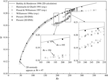
being the Strouhal number, see (A 4)) relationship over the laminar and 3D wake transition regimes is shown in figure 2, together with previous independent experimental and numerical results reported in the literature. The present 2D results agree well with the 2D results reported by Barkley & Henderson (Reference Barkley and Henderson1996). The unsteady 2D flow appears at
 $Re=47$
, which is consistent with the numerical results by Henderson (Reference Henderson1997) and Posdziech & Grundmann (Reference Posdziech and Grundmann2001), and very close to the experimental result of
 $Re=49$
by Williamson (Reference Williamson1996a
). The present 3D results are also in good agreement with the experimental results reported in the literature (figure 2). It is noticed that the predicted sudden drop of
 $St$
occurs at a considerably higher
 $Re$
(
 ${\sim}$
194) than the
 $Re$
(
 ${\sim}$
178) reported by Williamson (Reference Williamson1996a
). The
 $Re$
corresponding to the sudden drop of
 $St$
in the
 $St$
–
 $Re$
relationship is often identified as
 $Re_{cr}$
in the literature. As stated by Williamson (Reference Williamson1996b
), the earlier transition point in Williamson (Reference Williamson1996a
) is largely due to end contamination in the experiments. By eliminating the end contaminations, Williamson (Reference Williamson1996b
) obtained an
 $Re_{cr}$
of 194. The
 $Re_{cr}$
from the present DNS study based on the standard 3D mesh is also 194. This value is also close to the
 $Re_{cr}$
values of 188.5 (
 $\pm$
1.0), 190.2 (
 $\pm$
0.02) and 190.5 predicted through linear stability analysis by Barkley & Henderson (Reference Barkley and Henderson1996), Posdziech & Grundmann (Reference Posdziech and Grundmann2001) and Rao et al. (Reference Rao, Thompson, Leweke and Hourigan2013) respectively.
The
 $St$
–
 $Re$
relationship over the laminar and 3D wake transition regimes.

3 Numerical results
Numerical simulations have been carried out for
 $Re$
up to 300 in order to predict the wake transitions beyond
 $Re_{cr}$
, including the interactions of mode A* and mode B structures, and the disappearance of mode A* and transition to pure mode B states. The wake transitions are identified qualitatively through numerical flow visualizations and quantitatively through examining the dependence of various flow properties on
 $Re$
, e.g. Strouhal number, drag and lift force coefficients (A 2)–(A 3), base pressure coefficient (A 5), streamwise vorticity, streamwise enstrophy, spanwise flow velocity and spanwise disturbance energy. The normalized streamwise vorticity
 ${\it\omega}_{x}$
is defined as
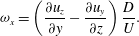 $$\begin{eqnarray}{\it\omega}_{x}=\left(\frac{\partial u_{z}}{\partial y}-\frac{\partial u_{y}}{\partial z}\right)\frac{D}{U}.\end{eqnarray}$$
The streamwise enstrophy
 ${\it\varepsilon}_{x}$
and spanwise disturbance energy
 $E_{z}$
are defined as
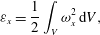 $$\begin{eqnarray}\displaystyle & \displaystyle {\it\varepsilon}_{x}=\frac{1}{2}\int _{V}{\it\omega}_{x}^{2}\,\text{d}V, & \displaystyle\end{eqnarray}$$
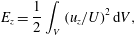 $$\begin{eqnarray}\displaystyle & \displaystyle E_{z}=\frac{1}{2}\int _{V}(u_{z}/U)^{2}\,\text{d}V, & \displaystyle\end{eqnarray}$$
 $V$
is the volume of the flow field of interest.
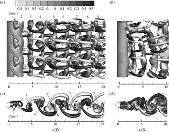
Isosurfaces of
 ${\it\lambda}_{2}=-0.05$
(coloured by
 ${\it\omega}_{x}$
) at
 $Re=220$
: (a)
 $t^{\ast }=200$
(with high mesh resolution for the entire wake); (b)
 $t^{\ast }=2600$
; (c) and (d) are the
 $z$
-normal views. The flow is from left to right passing through the cylinder on the left.

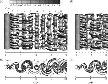
Isosurfaces of
 ${\it\lambda}_{2}=-0.05$
(coloured by
 ${\it\omega}_{x}$
) at
 $Re=300$
: (a)
 $t^{\ast }=160$
(with high mesh resolution for the entire wake); (b)
 $t^{\ast }=1820$
; (c) and (d) are the
 $z$
-normal views. The flow is from left to right passing through the cylinder on the left.

3.1 Vortex structures of modes A* and B
Before the examination of the complicated transition process from mode A* to mode B, which involves a mixture of the two modes and a mode swapping process, the vortex structures of the two modes are examined separately at
 $Re=220$
and
 $Re=300$
respectively, through numerical flow visualizations. The vortex cores are captured by the second negative eigenvalue
 ${\it\lambda}_{2}$
of the tensor
 ${\it\Psi}^{2}+{\it\Omega}^{2}$
, where
 ${\it\Psi}$
and
 ${\it\Omega}$
are the symmetric and antisymmetric parts of the velocity gradient tensor respectively (Jeong & Hussain Reference Jeong and Hussain1995). Figures 3 and 4 show the isosurfaces of
 ${\it\lambda}_{2}=-0.05$
(coloured by
 ${\it\omega}_{x}$
) at
 $Re=220$
(mode A) and
 $Re=300$
(mode B) respectively. From the visualization of the vortex structures, some particular features of the two modes, which are consistent with the experimental results reported in the literature (e.g. Williamson Reference Williamson1996b
), are summarized as follows.
-
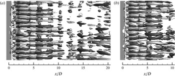
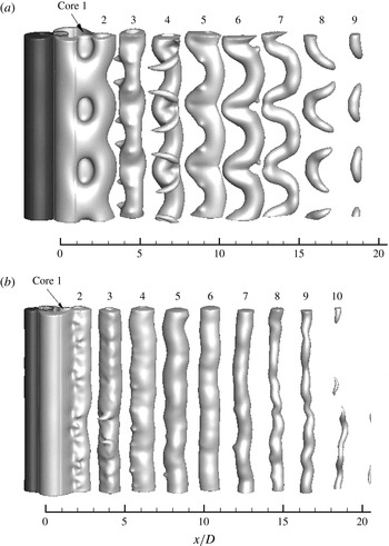
(1) The 3D wake patterns are characterized by the development of a pure mode A structure (figure 3 a) and a pure mode B structure (figure 4 a) at the early stages. However, the pure mode A structure only lasts for a short period of time before it evolves into a more stable pattern with large-scale dislocations, i.e. mode A* (figure 3 b), as observed by Williamson (Reference Williamson1996b ) and confirmed by numerical studies with different mathematical formulations (e.g. Henderson Reference Henderson1997; Braza et al. Reference Braza, Faghani and Persillon2001; Behara & Mittal Reference Behara and Mittal2010). After the evolution of dislocations, the primary vortices and streamwise vortex pairs become less regular and exhibit phase differences in the spanwise direction (figure 3 b). The dislocations can also be observed from the comparison of the Kármán vortex streets in the
 $z$
-normal view (figure 3
c,d). In contrast, the mode B structure does not contain large-scale dislocations (Williamson Reference Williamson1996b
). For instance, for the
$Re=300$
case, only pure mode B structure is observed for the whole simulation process (
$t^{\ast }=Ut/D=0{-}2440$
, with an output interval of 10) (see, e.g., the vortex structures at two distant steps shown in figure 4).
-
(2) It has been demonstrated in Williamson (Reference Williamson1996b ), Leweke & Williamson (Reference Leweke and Williamson1998) and Thompson, Leweke & Williamson (Reference Thompson, Leweke and Williamson2001) that the occurrence of mode A is due to an elliptic instability of the primary vortex cores and the formation of streamwise vortex pairs through Biot–Savart induction, whereas the occurrence of mode B is due to a hyperbolic instability of the braid shear layer region. In figure 3(a) (mode A), the wavy pattern of the primary vortex cores (labelled from 1 to 9) can be observed, and the streamwise vortex pairs are originated from the primary vortex cores. In figure 4(a) (mode B), the primary vortices (labelled from 1 to 10) are more stable, without large-scale spanwise waviness. It is also seen from the
$z$
-normal view that for mode A, the primary vortex cores have stretched projections due to spanwise waviness (figure 3
c), while for mode B, the projections of the primary vortices are in the shape of hollow circles, and the primary and streamwise vortices are largely independent of one another. -
(3) At
$Re=220$
(mode A), three streamwise vortex pairs are observed within the 12
$D$
spanwise range (figure 3
a), indicating a spanwise wavelength of approximately 4
$D$
. As pointed out by Williamson (Reference Williamson1996b
), the spanwise wavelength of the wavy primary vortex cores is naturally equal to the wavelength of the streamwise vortex pairs. In contrast, at
$Re=300$
(mode B), 14 streamwise vortex pairs are observed, resulting in a spanwise wavelength of approximately 0.86
$D$
(figure 4
a,b). It is found that the vortex pairs can be better visualized and counted from the isosurfaces of
${\it\omega}_{x}$
shown in figure 5. -
(4) The streamwise vortices of mode A exhibit an out-of-phase sequence between the neighbouring braids (figure 3 a), whereas an in-phase pattern is found in mode B (figure 5). This is consistent with the experimental findings reported by Williamson (Reference Williamson1996a ,Reference Williamson b ).
-
(5) Mode B can only be observed in the near wake (e.g. less than
$x=10D$
in figure 4
a), whereas mode A is sustainable for a much longer distance than mode B in the downstream direction (e.g. more than
$x=20D$
in figure 3
a). This is also consistent with the experimental findings reported by Williamson (Reference Williamson1996a
,Reference Williamson
b
).





Isosurfaces of
 ${\it\omega}_{x}=\pm 0.5$
at
 $Re=300$
: (a)
 $t^{\ast }=160$
(with high mesh resolution for the entire wake); (b)
 $t^{\ast }=1820$
. Dark and light grey denote positive and negative values respectively. The flow is from left to right passing through the cylinder on the left.

The isosurfaces of the pressure for
 $Re=220$
(mode A) and
 $Re=300$
(mode B) are shown in figure 6. It is seen that for both cases the high positive pressures occur at the front of the cylinder, while the negative values dominate the cylinder wake. The largest negative pressures mainly occur at the locations of the primary vortex cores. For mode A, the same wavy pattern for the primary vortex cores (figure 3
a) can be observed for the isosurfaces of the pressure (figure 6
a), and the same locations where three streamwise pairs develop along cores 2–4 in figure 6(a) are the locations of the streamwise vortex pairs in figure 3(a). For mode B, compared with mode A, the negative pressure is more concentrated at the primary vortex cores, and the streamwise pairs are less obvious.
Isosurfaces of pressure
 $p$
(with high mesh resolution for the entire wake): (a)
 $p=\pm 0.11$
at
 $Re=220$
and
 $t^{\ast }=200$
; (b)
 $p=\pm 0.20$
at
 $Re=300$
and
 $t^{\ast }=160$
. Dark and light grey denote positive and negative values respectively. The flow is from left to right passing through the cylinder on the left.

Williamson (Reference Williamson1996b
) demonstrated with 2D DNS results at
 $Re=200$
that the tearing of the primary vortex cores for mode A (see figure 3
a) is associated with the location of the saddle point observed in the flow. The saddle point indicates the location where strong straining occurs, causing part of the primary vortex downstream of the saddle point to be pulled back upstream (Williamson Reference Williamson1996b
). Williamson (Reference Williamson1996b
) stated that in the case of mode A, this primary vortex deformation occurs at particular spanwise locations where vortex loops are forming.
Locations of the saddle point and vortex centre identified from various
 $x$
–
 $y$
cross-sections at
 $Re=220$
and
 $t^{\ast }=200$
: (a) projections in the
 $x$
–
 $y$
plane (with isosurfaces of
 ${\it\lambda}_{2}=-2.0$
); (b) projections in the
 $x$
–
 $z$
plane (with isosurfaces of
 ${\it\lambda}_{2}=-1.0$
).

Cross-sectional flow field (with arrows indicating the flow direction) and spanwise vorticity contours at different spanwise locations for
 $Re=220$
and
 $t^{\ast }=200$
. The spanwise vorticity contours are shown at
 $|{\it\omega}_{z}|=2.0{-}3.0$
(illustrated in (a)) with an interval of 0.1. The saddle point is marked by a cross in the figure.

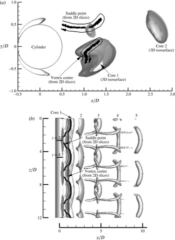
The above findings are confirmed in the present study using 3D DNS. Figure 7 shows the instantaneous locations of the saddle point and vortex centre identified from various
 $x$
–
 $y$
cross-sections (some are shown in figure 8) along with the isosurfaces of vortex cores determined by
 ${\it\lambda}_{2}$
, for the case of mode A at
 $Re=$
220. On combining the two perspectives shown in figure 7, it is seen that the locations of the saddle point along the span are regular periodic and have a spanwise periodicity of the same value (4
 $D$
) as for the wavy primary vortex cores and streamwise vortex pairs. When the saddle point gradually moves towards the cylinder, the primary vortex cores are also pulled back towards the cylinder, and the streamwise vortex pairs are developed at such spanwise locations (figure 7
b), which is consistent with the findings by Williamson (Reference Williamson1996b
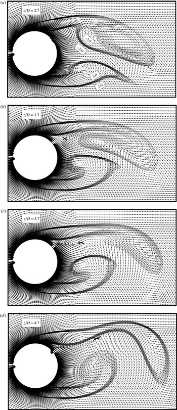
). Figure 8 shows four instantaneous 2D cross-sectional flow fields within half of a spanwise wavelength (
 $z/D=2.7{-}4.7$
), overlaid with contours of spanwise vorticity, which is defined as
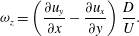 $$\begin{eqnarray}{\it\omega}_{z}=\left(\frac{\partial u_{y}}{\partial x}-\frac{\partial u_{x}}{\partial y}\right)\frac{D}{U}.\end{eqnarray}$$
At
 $z/D=4.7$
, the saddle point is furthest away from the cylinder. As the saddle point moves back towards the cylinder for
 $z/D$
from 4.7 to 3.3, part of the negative spanwise vortex as shown in figure 8 is pulled back towards the cylinder. The positive spanwise vortex also moves towards the cylinder, as well as being pushed downwards by the backward movement of the negative vortex. The tearing of the spanwise vortex was also observed by Williamson (Reference Williamson1996b
) with 2D DNS results. For
 $z/D$
from 3.3 to 2.7, the saddle point is not observed in the flow. The negative spanwise vortex moves further back towards the cylinder. As the vortex centre within the positive vortex is already very close to the cylinder, a more drastic downward movement is observed (see figure 7
a).
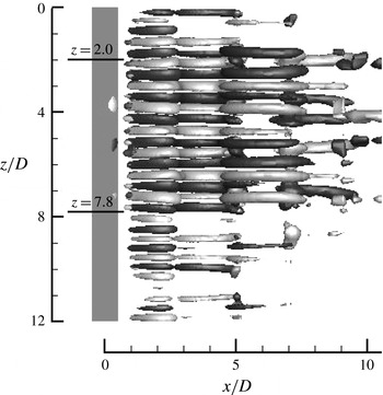
In the case of mode B, a regular mode B structure within
 $z/D=2.0{-}7.8$
at
 $Re=270$
and
 $t^{\ast }=3140$
(figure 9) is used for identifying the location pattern of the saddle point along the span. It will be shown in § 3.3 that mode B is most regular at approximately
 $Re=270$
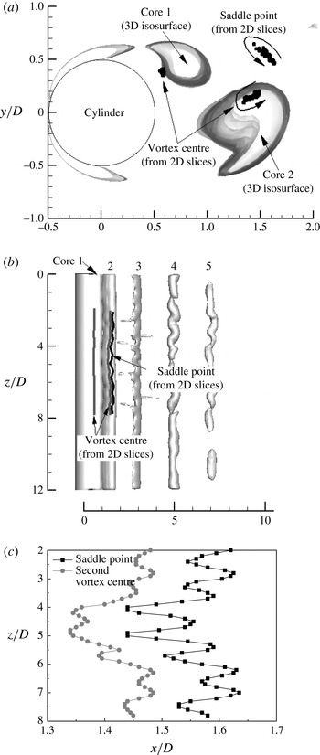
. Figure 10 shows the instantaneous locations of the saddle point and vortex centre identified from various
 $x$
–
 $y$
cross-sections along with the isosurfaces of vortex cores determined by
 ${\it\lambda}_{2}$
. From the close-up view of the
 $x$
–
 $z$
plane (figure 10
c), seven cycles of the variations of the saddle point and second vortex centre are observed within
 $z/D=2.0{-}7.8$
along the span, which is consistent with the seven streamwise vortex pairs shown in figure 9. Although the periodic cycles for mode B are not as regular as for mode A, it is still evident that the tearing of the primary vortex cores is associated with the location of the saddle point in very similar phase variations (figure 10
c). It is observed from the projections in the
 $x$
–
 $y$
plane that the variation range of the location of the saddle point for mode B (figure 10
a) is much smaller than that for mode A (figure 7
a). As a result, the primary vortex cores of mode B display much smaller spanwise waviness amplitudes.
Isosurfaces of
 ${\it\omega}_{x}=\pm 0.5$
at
 $Re=270$
and
 $t^{\ast }=3140$
. Dark and light grey denote positive and negative values respectively. The flow is from left to right passing through the cylinder on the left.

Locations of the saddle point and vortex centre identified from various
 $x$
–
 $y$
cross-sections at
 $Re=270$
and
 $t^{\ast }=3140$
: (a) projections in the
 $x$
–
 $y$
plane (with isosurfaces of
 ${\it\lambda}_{2}=-2.0$
); (b) projections in the
 $x$
–
 $z$
plane (with isosurfaces of
 ${\it\lambda}_{2}=-1.5$
); (c) close-up view of the
 $x$
–
 $z$
plane with the locations of the saddle point and vortex centre.

Frequency spectra of
 $C_{L}$
for
 $Re$
in the range of 200–300.

3.2 Transition from mode A* to mode B
3.2.1 Transition range
The second discontinuous change in the
 $St$
–
 $Re$
curve (figure 2), i.e. the transition from mode A* to mode B, occurs at approximately
 $Re=230{-}260$
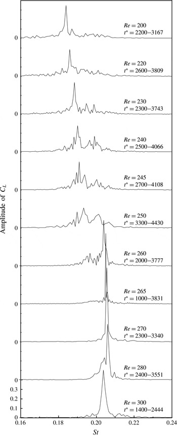
. The frequency spectra of
 $C_{L}$
over the transition range are shown in figure 11. For
 $Re\leqslant 220$
, a distinct peak which corresponds to mode A* exists in the spectrum. With the increase of
 $Re$
, a second peak with higher frequency which corresponds to mode B starts to grow. Meanwhile, the amplitude of the first peak decreases. The two peaks have similar amplitudes at approximately
 $Re=250$
. At
 $Re=260$
, the second peak becomes dominant, whereas the first peak decays further. Beyond
 $Re=265$
, the peak corresponding to mode A* vanishes almost completely and the one corresponding to mode B dominates the spectrum. The gradual energy transfer process from mode A* to mode B with the increase of
 $Re$
observed here confirms the experimental finding by Williamson (Reference Williamson1988). A similar process was also observed in a recent numerical study by Behara & Mittal (Reference Behara and Mittal2010). The numerical results shown in figure 11 indicate that the transition process from mode A* to mode B occurs in the range of
 $Re$
from 230 to 260, which is quite close to the range of
 $Re=230{-}250$
reported by Williamson (Reference Williamson1996a
) through experiments and the ranges of 230–265 (Barkley et al.
Reference Barkley, Tuckerman and Golubitsky2000) and 230–260 (Sheard et al.
Reference Sheard, Thompson and Hourigan2003) based on nonlinear stability analysis.
It is also seen from figure 11 that the frequency peaks are accompanied by small fluctuations for
 $Re\leqslant 260$
. According to Henderson (Reference Henderson1997), this is due to the occurrence of vortex dislocations associated with mode A*, which leads to a broadband frequency spectrum. In particular, in the mode swapping regime, small fluctuations are observed around the two frequency peaks. At the beginning and end of the transition process (i.e. at
 $Re=230$
and 260), the secondary shedding mode is rather weak. Therefore, only the primary peak frequency is identified and plotted in the
 $St$
–
 $Re$
curve shown in figure 2. For the three cases in between, both peak frequencies can be captured and are thus plotted in the
 $St$
–
 $Re$
curve (see the close-up view in figure 2).
It is worth noting that an accurate determination of the relative importance (probability of occurrence) of mode A* and mode B is difficult to achieve based on the frequency spectra shown in figure 11. This is because the broadband frequency spectra due to mode A* (Henderson Reference Henderson1997) may interfere with the frequency peak of mode B. For example, the frequency spectra of
 $Re=200$
and 220 (figure 11) are due to mode A* only, but contain small fluctuations spanning a range of
 $St$
from
 ${\sim}0.16$
to 0.21, covering the
 $St$
range for mode B. Therefore, it is difficult to decouple the frequency peaks contributed by the two modes and to divide the range of
 $St$
for the two modes precisely. Alternatively, the probability of occurrence of mode A* and mode B may be determined through numerical flow visualization, which will be examined later on in this section.
Nevertheless, since the mode A* frequency peak becomes relatively weak at
 $Re\geqslant 250$
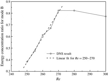
, the mode B frequency peak becomes less contaminated by mode A* and better distinguished, and thus the concentration of the energy in the mode B peak can be roughly quantified. Figure 12 shows the variation of the energy concentration ratio for mode B with
 $Re$
. The energy concentration ratio is defined as the ratio of the area under the mode B peak to the area under the entire frequency spectrum of
 $St$
between 0.16 and 0.24 shown in figure 11. The width of the area under the mode B peak is chosen as
 ${\rm\Delta}St=0.1$
(so that the mode A* peak is not incorporated), with the centre located at the peak frequency point. It is seen in figure 12 that the energy concentration ratio for mode B generally increases linearly with
 $Re$
for
 $Re=250{-}270$
but decreases slightly with further increase of
 $Re$
(as the mode B structure becomes increasingly disordered at
 $Re>270$
, which will be shown later on in § 3.2.3).
As
 $Re$
increases from 200 up to 280, the frequencies corresponding to both peaks increase gradually. The frequency corresponding to mode B experiences a slight drop as
 $Re$
increases from 280 to 300 (see figures 2 and 11). It is also noticed that the
 $St$
values predicted by the 2D and 3D simulations are closest to each other at
 $Re=270$
after the onset of mode A* instability (see figure 2). The physical reasons behind this feature will be discussed in § 3.3.
Variation of the energy concentration ratio for mode B with
 $Re$
.

Probability of occurrence of mode A* and mode B structures.

The transient vortex structures in the transition from mode A* to mode B are examined visually. Figure 13 shows the variations of the probability of occurrence of two vortex patterns with
 $Re$
: (1) mode A* (with large-scale dislocations, not pure mode A), and (2) mode B structures. The probability of occurrence of mode A* or mode B structures is defined as the ratio of the accumulated time of appearance of the mode to the total sampling time. The statistics for the probability of occurrence normally starts at
 $t^{\ast }=1000$
(with an output interval of 10), where the flow is fully developed. For the cases in the transition regime, normally 175–355 snapshots of the
 ${\it\omega}_{x}$
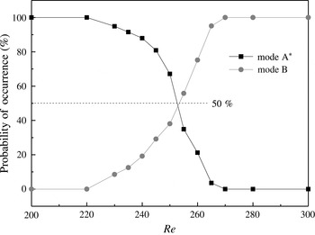
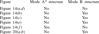
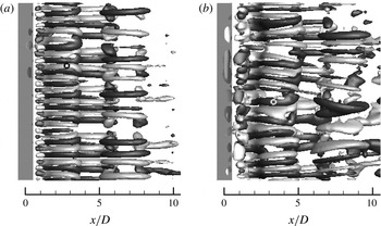
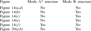
field are examined for each case to achieve meaningful (sample-independent) statistics. For each case, the statistics is carried out by visually examining the existence of the above vortex patterns in each snapshot. The large-scale dislocations are spotted easily as they appear in the form of continuous periods and normally take up the entire span width. The mode B pattern, on the other hand, is largely scattered around across the span width and is less obvious. It should be noted that the mode B pattern is only counted when there exist at least two successive mode B streamwise vortex pairs along the span width. For further clarity, a few examples are given in table 1 to illustrate the identification of mode A* and mode B with reference to the wake patterns shown in figures 14 and 20.
A short sequence of the isosurfaces of
 ${\it\omega}_{x}=\pm 0.5$
at
 $Re=240$
. Dark and light grey denote positive and negative values respectively. The flow is from left to right passing through the cylinder on the left.

Examples of the classification of wake patterns based on the streamwise vorticity field.
It is found that for
 $Re\leqslant 220$
, only dislocation patterns exist in the domain and there is no sign of mode B (see, e.g., figure 3
b). For
 $Re\geqslant 270$
, vortex dislocations do not occur, whereas only mode B (and sometimes together with scattered pure mode A) can be observed in all of the snapshots examined (see, e.g., figure 4). During the transition process of
 $Re$
between 230 and 265, however, both vortex patterns can be detected in the simulations. The two patterns usually occur at different time instants as the dislocations can normally occupy the whole span width. Occasionally, they may coexist in the same domain (but at different spanwise locations). With the increase of
 $Re$
, the probabilities of occurrence of mode A* and mode B exhibit monotonic drop and growth respectively. The two probability curves intersect at approximately
 $Re=253$
with the probability of occurrence of either mode of approximately 50 % (figure 13). This point is thus considered as the separation point beyond which mode B becomes dominant.
Based on the observation of a sharp decrease of the statistical width of the wake structure at
 $Re\sim 250$
when mode B appears, Williamson (Reference Williamson1996b
) suggested that this ‘possibly corresponds with a decrease in the presence of dislocations’. Through numerical visualization of the transient vortex structures, the present study confirms clearly the decrease of probability of occurrence of dislocations (i.e. mode A*) with increase of
 $Re$
. However, unlike the indication of a discontinuous decrease of the wake width as shown in Williamson (Reference Williamson1996b
), the decrease of the probability of occurrence of dislocations observed in figure 13 is a continuous process. Considering that the decreasing trend mainly occurs in a narrow
 $Re$
range of 240–265 (figure 13), the experiments carried out in Williamson (Reference Williamson1996b
) with an
 $Re$
interval of
 ${\sim}15$
may be the reason why a continuous decreasing trend was not identified.
The transition process observed visually (figure 13) shows some similarities with that observed through examining the frequency spectra of
 $C_{L}$
(figure 11) in terms of the transition range and relative importance of the two modes. At
 $Re=265$
, the frequency spectra of
 $C_{L}$
cannot capture the mode A* peak, whereas, based on visualization, the mode A* pattern has a very small probability of occurrence of 3.5 %. It should be noted that in this case the dislocations only occur during
 $t^{\ast }=1540{-}1630$
, and cannot be observed during the remaining simulation period of more than 2000 non-dimensional time units. Based on the present simulation results, it is reasonable to say that
 $Re=265$
is just within or beyond the range of the transition process from mode A* to mode B.
3.2.2 Mode swapping cycles in the transition range
In the transition process from mode A* to mode B, mode swapping occurs cyclically in each case. Each mode cycle begins with the emergence of a nearly pure mode A structure along the entire span width. The pure mode A structure develops in strength for a short period of time, followed by one of the following two routes.
-
(1) Dislocation cycle. The pure mode A structure evolves into a continuous stage of mode A* (i.e. with large-scale dislocations). The dislocation stage may last for some time before it is replaced by the pure mode B structure or a mixture of modes B and A (without dislocations). It should be noted that in the mixture of modes B and A, mode A emerges intermittently at random spanwise locations, but cannot fill up the whole span width, and will be replaced by mode B shortly.
-
(2) Non-dislocation cycle. The pure mode A structure is replaced by mode B directly, followed by the persistence of the pure mode B structure or a mixture of modes B and A (without dislocations). It should be noted that for a non-dislocation cycle, there are no dislocations throughout the whole cycle.
At the end of each cycle, all of the mode B structures die off. If the cycle ends with the pure mode B structure spanning the entire span width, the wake will become almost 2D. If the cycle ends with a mixture of modes B and A (without dislocations), the mode B structure in the mixture will die off while the mode A structure in the mixture will form part of the pure mode A structure in the next cycle. Eventually, a new cycle with the development of a pure mode A structure along the entire span width begins.
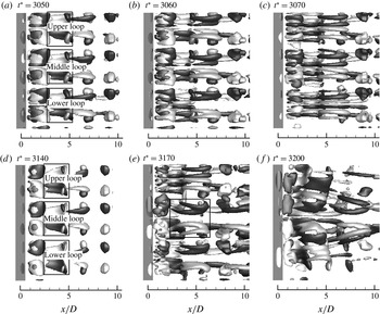
Figure 14 shows a typical short sequence of the development of
 ${\it\omega}_{x}$
field extracted from the case of
 $Re=240$
. In the first cycle (figure 14
a–c), after the formation of a pure mode A structure with three streamwise vortex pairs (figure 14
a), mode B starts to develop within the three vortex loops (figure 14
b) and gradually fills up the whole span width (figure 14
c). In the second cycle (figure 14
d–f), after the emergence of the same mode A structure as that in the first cycle (figure 14
d), vortex dislocation starts to occur in the middle loop (as marked by a solid rectangle frame in figure 14
e) and propagates towards both ends of the span until the whole span is occupied by large-scale dislocations (figure 14
f). It is seen that although the upper loop is fully occupied by mode B structures in figure 14(e), which is similar to the process observed in the first cycle, the dislocation originated from the middle loop eventually engulfs all mode B structures, leading to a dislocation structure across the entire span area.
The two cycles described in the previous paragraph actually take two different routes despite the similar initial conditions shown in figure 14(a,d). As long as dislocations occur within any of the three mode A vortex loops, the mode swapping cycle will follow the dislocation cycle, no matter what happens to the rest of the loops. A non-dislocation cycle can only occur when all of the loops are filled with mode B structures, either simultaneously or successively. This conclusion is found to be valid in the entire transition process from mode A* to mode B, and all of the large-scale dislocations observed in the transition process from mode A* to mode B are initialized with the local dislocation (spanwise modulation) of a specific vortex loop in the domain (after the pure mode A structure develops in strength for a short period of time).
As stated in Henderson (Reference Henderson1997), the mode B structures observed during the transition process from mode A* to mode B (
 $Re=230{-}260$
), prior to the onset point of mode B instability predicted through linear stability analysis (e.g.
 $Re=259$
by Barkley & Henderson (Reference Barkley and Henderson1996)), are due to the fact that the existence of mode A* instability would destabilize mode B in the nonlinear interaction between the two modes. Through numerical flow visualization of the whole transition process from mode A* to mode B, it is found that all of the mode B structures are developed based on the streamwise vortex pairs of mode A (see, e.g., figure 14) or streamwise vortices of mode A*. Since the physical mechanism for mode B instability is a hyperbolic instability of the braid shear layer region (Williamson Reference Williamson1996b
; Leweke & Williamson Reference Leweke and Williamson1998; Thompson et al.
Reference Thompson, Leweke and Williamson2001), it is believed that the streamwise vortices of modes A and A* developed in the braid shear layer region are the destabilization factors for an early development of the mode B structures. After the replacement of the streamwise vortices of mode A or A* by mode B, the mode B structures may decay in time, as the source for the destabilization of mode B disappears. However, due to the intermittent emergence of the mode A streamwise vortex pairs which fill up the locations where mode B disappears, a mixture of modes B and A is sustained before the end of a cycle.
Time histories of the occurrence of dislocations for the cases in the transition process from mode A* to mode B.

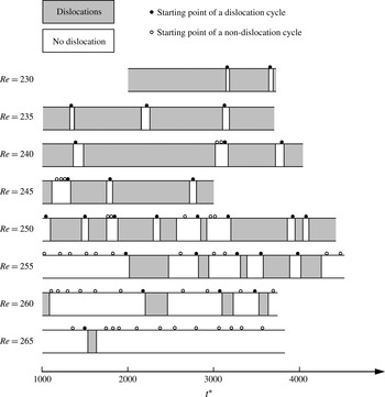
Figure 15 shows the mode swapping process as a function of time for the cases in the transition process from mode A* to mode B. The starting point of each dislocation and non-dislocation cycle is denoted by a solid dot and open circle respectively. For each dislocation cycle beginning with a solid dot, a shaded dislocation period is followed (figure 15). For
 $Re$
ranging from 230 to 245, the non-dislocation cycles are very short in duration while the dislocation periods persist for at least 400 non-dimensional time units. As a result, the probability of occurrence of the large-scale dislocations is larger than 80 %, whereas for the mode B structures which largely occur in the non-dislocation segments, the probability of occurrence is smaller than 30 % (see figure 13). At
 $Re=250$
, the average duration of the dislocation periods drops sharply to 284 non-dimensional time units, and more dislocation cycles can be observed. The cyclic mode swapping process becomes more frequent. With decrease of the lengths of the dislocation cycles, the probability of occurrence of dislocations decreases and the probability of occurrence of mode B structures increases (figure 13).
For
 $Re$
ranging from 230 to 250, the dislocation cycles can be triggered easily from the pure mode A structure within one to four cycles. For
 $Re$
ranging from 255 to 265, it becomes relatively difficult to trigger dislocations from the pure mode A structure, as it is seen in figure 15 that there are many more non-dislocation cycles than dislocation cycles. In addition, compared with the average duration of the dislocation periods at
 $Re=250$
(of 284 non-dimensional time units), the average durations of the dislocation periods at
 $Re=255$
, 260 and 265 are further reduced to 248, 167 and 100 non-dimensional time units respectively. For
 $Re\geqslant 260$
, the non-dislocation cycles have similar durations to the dislocation cycles. As a result, for
 $Re\geqslant 260$
, the probability of occurrence of large-scale dislocations is smaller than 25 %, while the probability of occurrence of mode B structures is larger than 75 %.
Beyond
 $Re=270$
, there are no mode swapping cycles. The only case with the occurrence of mode A (without dislocations) is the
 $Re=270$
case, in which a mixture of modes B and A (without dislocations) is observed.
3.2.3 Time histories of the force coefficients and vorticity
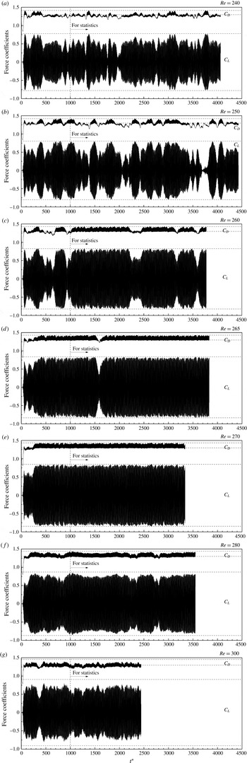
Figure 16 plots the time histories of the drag and lift force coefficients for a few cases that contain mode B. The horizontal dashed lines in each figure mark the fluctuation ranges of the corresponding 2D force coefficients. For the cases in the transition process from mode A* to mode B (figure 16
a–c), it is seen that the periods over which large amplitudes of
 $C_{L}$
take place match the non-dislocation periods shown in figure 15. The amplitudes of
 $C_{D}$
and
 $C_{L}$
observed during the non-dislocation periods are close to their 2D counterparts, indicating that the flow three-dimensionality is weak when dislocations do not occur. During the dislocation periods, the
 $C_{D}$
values and the amplitudes of
 $C_{L}$
decrease, indicating that energy is transferred to the third direction. In particular, oblique vortex shedding occurs spontaneously along the entire span at
 $t^{\ast }=3710{-}3820$
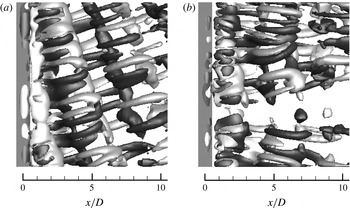
for the
 $Re=250$
case (e.g. figure 17
a, in comparison with an example of parallel vortex shedding shown in figure 17
b). Due to the remarkable phase differences along the span, the integrated lift coefficient is largely cancelled out, resulting in the smallest fluctuation amplitudes in the time history (figure 16
b).
Time histories of the drag and lift coefficients for some cases containing mode B.

Isosurfaces of
 ${\it\omega}_{x}=\pm 0.5$
at
 $Re=250$
: (a) oblique vortex shedding at
 $t^{\ast }=3750$
; (b) parallel vortex shedding at
 $t^{\ast }=3850$
. Dark and light grey denote positive and negative values respectively. The flow is from left to right passing through the cylinder on the left.

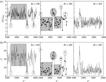
The relationship between dislocation and the degree of flow three-dimensionality is further examined with both the largest
 $|{\it\omega}_{x}|$
value in the domain and the streamwise enstrophy
 ${\it\varepsilon}_{x}$
integrated over the near-wake region of
 $x/D=0{-}10$
. At
 $Re=240$
, for each of the three non-dislocation periods shown in figure 15, there is a sudden drop in the time histories, as highlighted with a circle in the left column of figure 18. At
 $Re=260$
, each of the four dislocation periods corresponds to a rapid increase of
 $|{\it\omega}_{x}|_{max}$
and
 ${\it\varepsilon}_{x}$
, as circled in the middle column of figure 18. The non-dislocation and dislocation parts can be roughly divided by the horizontal line of
 $|{\it\omega}_{x}|_{max}=4.5$
as shown in figure 18(a). For the
 $Re=265$
case, the entire time histories beyond the only dislocation period of
 $t^{\ast }=1540{-}1630$
are generally below the division line, as shown in the right column of figure 18.
Time histories of (a) the largest
 $|{\it\omega}_{x}|$
value in the domain and (b) the streamwise enstrophy
 ${\it\varepsilon}_{x}$
integrated over the near-wake region of
 $x/D=0{-}10$
for some cases in the transition process from mode A* to mode B.

During the transition process from mode A* to mode B, the mode B structure, which is largely observed in the non-dislocation segments with large-amplitude force coefficients, usually takes up part of the span, and the streamwise vortices are quite ordered (e.g. figure 14
c,e). At
 $Re$
of 265 (beyond the only dislocation period) and 270, the large-amplitude force coefficients resemble the 2D results for the entire fully developed stage (figure 16
d,e). The mode B structure is also in an ordered pattern, and can normally occupy the majority of the span. Beyond
 $Re=270$
, mode B becomes increasingly disordered with increase of
 $Re$
. Correspondingly, the force coefficients deviate more and more from their 2D counterparts and become increasingly disordered (figure 16
f,g).
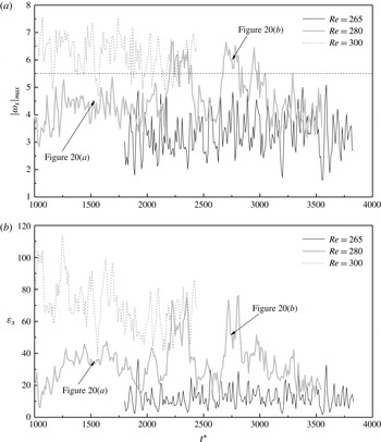
As mode B becomes increasingly disordered beyond
 $Re=270$
, the largest
 $|{\it\omega}_{x}|$
value and integrated
 ${\it\varepsilon}_{x}$
in the domain, which represent the degree of flow three-dimensionality, also increase with increase of
 $Re$
(figure 19). Generally speaking, the streamwise vortices are found to be more disordered when
 $|{\it\omega}_{x}|_{max}>5.5$
. It is seen from figure 19 that disordered mode B can sometimes occur at
 $Re=280$
(when
 $|{\it\omega}_{x}|_{max}>5.5$
). Figure 20 gives some examples of typical ordered and relatively disordered mode B patterns at
 $Re=280$
. The corresponding
 $|{\it\omega}_{x}|_{max}$
values of the two time instants are pointed out in figure 19. For the ordered one shown in figure 20(a), the streamwise vortices are all parallel to each other in the streamwise direction and have similar spanwise wavelengths. In contrast, the disordered mode B as shown in figure 20(b) contains slightly oblique streamwise vortices, and their spanwise wavelengths are rather different. At
 $Re=300$
, disordered mode B similar to the pattern shown in figure 20(b) occurs more frequently, whereas relatively ordered mode B structures (e.g. figure 5) only occur occasionally. In this case, the majority part of the time history of
 $|{\it\omega}_{x}|_{max}$
shown in figure 19(a) is above the horizontal line of
 $|{\it\omega}_{x}|_{max}=5.5$
.
Time histories of (a) the largest
 $|{\it\omega}_{x}|$
value in the domain and (b) the streamwise enstrophy
 ${\it\varepsilon}_{x}$
integrated over the near-wake region of
 $x/D=0{-}10$
for some cases beyond the transition process from mode A* to mode B.

Isosurfaces of
 ${\it\omega}_{x}=\pm 0.5$
at
 $Re=280$
: (a) ordered mode B at
 $t^{\ast }=1550$
; (b) relatively disordered mode B at
 $t^{\ast }=2750$
. Dark and light grey denote positive and negative values respectively. The location of the largest
 $|{\it\omega}_{x}|$
value in the domain is denoted by a circle. The flow is from left to right passing through the cylinder on the left.

3.3 Critical condition at
$Re=265{-}270$

Williamson (Reference Williamson1996b
) reported a critical condition at
 $Re=260$
where maximum values of the base pressure coefficient and root-mean-square flow velocity were observed. The critical condition is confirmed in the present study at approximately
 $Re=265{-}270$
in terms of various quantities including flow velocity, vorticity and hydrodynamic forces.
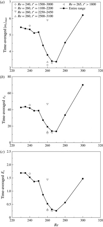
Figure 21(a) shows the variation of the time-averaged
 $|{\it\omega}_{x}|_{max}$
calculated from the time histories (e.g. figures 18
a and 19
a) with
 $Re$
. For
 $Re\leqslant 250$
, as mentioned previously, the relatively large
 $|{\it\omega}_{x}|_{max}$
values (i.e. strong flow three-dimensionality) are due to large-scale dislocations. A sharp drop of the
 $|{\it\omega}_{x}|_{max}$
is observed at
 $Re=250{-}265$
, in line with a sharp decrease of the probability of occurrence of dislocations as shown in figure 13. The averaged
 $|{\it\omega}_{x}|_{max}$
values obtained from a dislocation period and two non-dislocation periods (as shaded in figure 18) are further plotted in figure 21 to clarify the sharp drop. The non-dislocation periods that consist of either ordered mode B or mode A induce the lowest averaged
 $|{\it\omega}_{x}|_{max}$
values which are close to the one observed at
 $Re=270$
. In contrast, the averaged
 $|{\it\omega}_{x}|_{max}$
value observed during the dislocation period is much larger and is similar to the value observed in the dislocation period of
 $Re=240$
(as indicated by the shaded rectangle in the left column of figure 18). However, because the probabilities of occurrence of dislocations for
 $Re=260$
and
 $Re=240$
have a drastic difference (21.2 % and 88.0 % respectively), the overall averaged
 $|{\it\omega}_{x}|_{max}$
is very close to the dislocation value for
 $Re=240$
, but much closer to the non-dislocation values for
 $Re=260$
. At
 $Re=265$
, dislocations only have a very small probability of occurrence of 3.5 % and thus only have a very small effect on the overall performance. Beyond
 $Re=270$
, there is no dislocation in the domain, whereas the increasingly disordered mode B becomes the reason why the averaged
 $|{\it\omega}_{x}|_{max}$
starts to grow again. Figure 21(b,c) shows the variations of the time-averaged
 ${\it\varepsilon}_{x}$
and
 $E_{z}$
within
 $x/D=0{-}10$
of the wake with
 $Re$
. It is seen that all of the three quantities share similar trends in terms of predicting the three-dimensionality of the flow.
Time-averaged quantities for the 3D cases: (a) the largest
 $|{\it\omega}_{x}|$
value in the domain; (b) the integrated streamwise enstrophy within
 $x/D=0{-}10$
; (c) the integrated spanwise kinetic energy within
 $x/D=0{-}10$
.

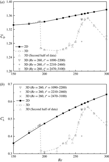
Figure 22 shows the time-averaged drag coefficient and root-mean-square lift coefficient for a wide range of
 $Re$
. The statistics is taken after the flow becomes fully developed. For the time histories shown in figure 16, the statistics starts at
 $t^{\ast }=1000$
. The results calculated from the second half of the sampling period are also plotted in figure 22 to demonstrate the sufficiency of the statistical data. At
 $Re=194$
, the deviations of the 3D
 $\overline{C_{D}}$
and
 $C_{L}^{\prime }$
results from the 2D curves mark the onset of mode A* instability. It is seen in figure 22 that the flow three-dimensionality becomes weakest at
 $Re$
of 265 and 270, in line with the variation trends of the time-averaged
 $|{\it\omega}_{x}|_{max}$
,
 ${\it\varepsilon}_{x}$
and
 $E_{z}$
(figure 21). The
 $\overline{C_{D}}$
and
 $C_{L}^{\prime }$
values at
 $Re=260$
can also be separated into the dislocation and non-dislocation parts (figure 22), in the same way as the separation of the time-averaged
 $|{\it\omega}_{x}|_{max}$
,
 ${\it\varepsilon}_{x}$
and
 $E_{z}$
values.
Time-averaged drag coefficient and root-mean-square lift coefficient.

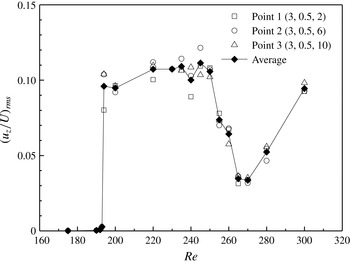
Figure 23 shows the root-mean-square spanwise velocity recorded at three sampling points in the near wake. As the
 $\overline{C_{D}}$
and
 $C_{L}^{\prime }$
values drop from their 2D counterparts after the onset of mode A* instability (figure 22), the fluctuations of the spanwise velocity grow accordingly. The same sharp drop at
 $Re$
of 265 and 270 is observed in figure 23 due to a weaker flow three-dimensionality, which is consistent with the variations observed in figures 21 and 22.
Root-mean-square spanwise velocity recorded at three sampling points in the near wake.

The same variation trends can also be observed in the
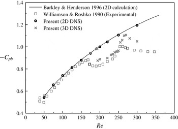
 $St$
–
 $Re$
(figure 2) and
 $C_{pb}$
–
 $Re$
(figure 24) relationships, where the 2D and 3D values are closest to each other at approximately
 $Re=265{-}270$
. It should be noted that in the
 $C_{pb}$
–
 $Re$
curve, the sudden drop observed at the transition to mode A* instability is different from the experimental result by Williamson & Roshko (Reference Williamson and Roshko1990), in terms of both the critical point and the shape of the curve near the critical point. As reported by Williamson (Reference Williamson1996b
), the critical transition point should be at approximately
 $Re=194$
if the end contamination effect is well controlled. Regarding the shape of the curve, since the
 $St$
–
 $Re$
curve (figure 2) also exhibits a sudden drop rather than a mild decrease at the transition to mode A* instability, it is believed that a sudden drop may take place for the base pressure coefficient as well.
Variation of the base pressure coefficient with the Reynolds number over the laminar and 3D wake transition regimes.

The critical condition at approximately
 $Re=265{-}270$
as discussed above has also been pointed out by Williamson (Reference Williamson1996b
), in which the critical point was reported to be at
 $Re=260$
. For example, the experimental study by Williamson & Roshko (Reference Williamson and Roshko1990) found that the peak in the base pressure curve was at approximately
 $Re=260$
(figure 24). Two possible causes were proposed by Williamson (Reference Williamson1996b
). One is due to the resonance between the shear layer oscillations and the wake oscillations at approximately
 $Re=262$
. The other is that the whole span becomes unstable to mode B at this point, rather than the presence of patches of mode B together with mode A and dislocations. On the other hand, the numerical study by Henderson (Reference Henderson1997) related this phenomenon solely to the nonlinear stability of mode B.
According to the discussion in this section, we suggest that the critical condition at approximately
 $Re=265{-}270$
marks a transition from the disappearance of the large-scale dislocations associated with mode A* to the emergence of increasingly disordered mode B structures, leading to the weakest flow three-dimensionality in this region. The present numerical results show that the flow structure at the critical condition of
 $Re=265{-}270$
is characterized by a mixture of ordered mode B and mode A structures, rather than only pure mode B structures. Similar mixed ordered flow structures and weakest flow three-dimensionality are also found in the non-dislocation periods at
 $Re=260$
. It is the additional dislocation periods that divert the overall time-averaged quantities in figures 21–24 away from the critical condition.
4 Conclusions
This paper presents detailed 3D DNS of flow past a circular cylinder over a range of
 $Re$
up to 300. The high-resolution vortex structures of mode A, mode A* and mode B have been reproduced by DNS. It is demonstrated with 3D DNS that the periodic tearing of the primary vortex cores is associated with the spanwise periodicity of the location of the saddle point in the flow. It is found that the variation range of the location of the saddle point for mode B is much smaller than that for mode A, which is responsible for much smaller spanwise waviness amplitudes of the primary vortex cores of mode B in comparison with mode A.
The gradual wake transition process from mode A* to mode B (Williamson Reference Williamson1996b
) is well captured over a range of
 $Re$
from 230 to 260. With increase of
 $Re$
, the probabilities of occurrence of mode A* and mode B exhibit continuous and monotonic drop and growth respectively. Mode B becomes the dominant mode beyond
 $Re\sim 253$
. For each case within the transition range, the transient mode swapping process consists of dislocation and non-dislocation cycles. Each cycle begins with a nearly pure mode A structure, followed by a stage of mode A* and then a stage of mode B or a mixture of modes B and A (without dislocations) for a dislocation cycle, or a stage of mode B or a mixture of modes B and A (without dislocations) directly for a non-dislocation cycle. With increase of
 $Re$
, it becomes more difficult to trigger dislocations from the pure mode A structure and form a dislocation cycle, and each dislocation stage becomes shorter in duration, resulting in a continuous reduction in the probability of occurrence of mode A* and thus an opposite effect for mode B. The occurrence of large-scale dislocations results in a decrease of the drag coefficient, a decrease of the amplitude of the lift coefficient and an increase of the largest streamwise vorticity and integrated streamwise enstrophy in the domain, indicating strong flow three-dimensionality.
The mode B structures in the transition process are developed based on the streamwise vortices of mode A or A* which destabilize the braid shear layer region. After the replacement of the streamwise vortices of mode A or A* by mode B, the mode B structures may decay in time, as the source for the destabilization of mode B disappears. However, due to the intermittent emergence of the mode A streamwise vortex pairs which fill up the locations where mode B disappears, a mixture of modes B and A is sustained before the end of a cycle.
A critical condition (Williamson Reference Williamson1996b
) is confirmed by the present DNS at approximately
 $Re=265{-}270$
, where the weakest flow three-dimensionality is observed. The weakest flow three-dimensionality at this point is reflected by the smallest time-averaged
 $|{\it\omega}_{x}|_{max}$
,
 ${\it\varepsilon}_{x}$
and
 $E_{z}$
values in the domain, the smallest root-mean-square spanwise velocity in the near wake, and the closest 2D and 3D results of the mean drag coefficient, root-mean-square lift coefficient, Strouhal number and base pressure coefficient. A transition from the disappearance of mode A* to the emergence of increasingly disordered mode B structure is responsible for this critical condition.
Acknowledgements
This work was supported by resources provided by the Pawsey Supercomputing Centre with funding from the Australian Government and the Government of Western Australia. The first author would like to acknowledge the support from the Australian Government and the University of Western Australia by providing IPRS and APA scholarships for a doctoral degree, as well as the Australia–China Natural Gas Technology Postgraduate Research Scholarships from the Australian and Western Australian Governments, the North West Shelf Joint Venture Partners and the Western Australian Energy Research Alliance. The fourth author would like to acknowledge the support from the Australian Research Council through Discovery Early Career Research Award (DE150100428).
Appendix A
The computational mesh and domain size were chosen based on a parameter dependence check, which was carried out in two steps. (i) First, the adequacy of mesh resolution and domain size in the
 $x$
–
 $y$
plane (i.e. the plane perpendicular to the cylinder span) was examined by a number of 2D simulations. (ii) A 3D mesh was generated by replicating an adequate 2D mesh along the
 $z$
-axis, resulting in an identical mesh resolution in all planes perpendicular to the cylinder span. A mesh dependence study on this mesh was then undertaken. The selected 2D mesh and the resulting 3D mesh are referred to as the standard meshes throughout this paper.
A reference 2D mesh was constructed first based on a preliminary parameter dependence study, which is not detailed here. The domain size for the reference mesh is
 $50D\times 40D$
. The cylinder perimeter is equally discretized with 132 nodes. The radial size of the first layer of mesh next to the cylinder is 0.001
 $D$
. The cell expansion ratio in the whole domain is kept below 1.1. A close-up view of the reference mesh near the cylinder is shown in figure 1(b).
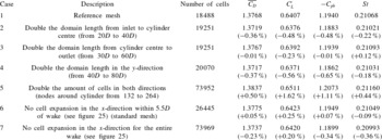
The reference mesh was used to simulate flow at
 $Re=300$
(case 1 in table 2), which is representative of the highest
 $Re$
adopted in this study. A total of six variations to the reference mesh were also used to simulate flow at
 $Re=300$
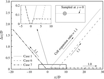
(cases 2–7 in table 2) so as to properly assess the adequacy of the mesh and domain size. Test cases 2–4 were designed to examine the adequacy of the computational domain size while test cases 6–7 were designed to examine the effect of mesh resolution in the wake region. The variation of cell length with
 $x$
-coordinate along
 $y=0$
is shown in figure 25. Case 5 doubles the number of cells of case 1 in both directions, which results in the finest overall mesh resolution among the cases considered. Specifically, the number of cells around the cylinder is doubled, while the radial size of the first layer of mesh next to the cylinder is halved.
Variation of cell length with
 $x$
-coordinate along
 $y=0$
.

Results of the 2D mesh dependence study at
 $Re=300$
. The relative errors in the brackets are calculated by using the results from case 1 as reference values.

The time step
 ${\rm\Delta}t$
adopted for each case is based on the criterion that the Courant number
 $Co$
is kept below 0.5 in the entire computational domain, where
 $Co$
is defined as
 $$\begin{eqnarray}\displaystyle Co=|u|{\rm\Delta}t/{\rm\Delta}l, & & \displaystyle\end{eqnarray}$$
where
 $|u|$
is the magnitude of the velocity through a cell and
 ${\rm\Delta}l$
is the cell size in the direction of the velocity. This results in a non-dimensional time step (defined as
 ${\rm\Delta}t^{\ast }=U{\rm\Delta}t/D$
) of
 $6.42\times 10^{-3}$
at
 $Re=300$
.
The mesh and domain size dependence was examined by quantifying the influence of domain size and mesh resolution on the drag and lift force coefficients (
 $C_{D}$
and
 $C_{L}$
), Strouhal number
 $St$
and base pressure coefficient
 $C_{pb}$
on the cylinder, which are defined as follows:
 $$\begin{eqnarray}\displaystyle & \displaystyle C_{D}=F_{D}/({\it\rho}DU^{2}L_{z}/2), & \displaystyle\end{eqnarray}$$
 $$\begin{eqnarray}\displaystyle & \displaystyle C_{L}=F_{L}/({\it\rho}DU^{2}L_{z}/2), & \displaystyle\end{eqnarray}$$
 $$\begin{eqnarray}\displaystyle & \displaystyle St=f_{L}D/U, & \displaystyle\end{eqnarray}$$
 $$\begin{eqnarray}\displaystyle & \displaystyle C_{pb}=(p_{b}-p_{\infty })/({\it\rho}U^{2}/2), & \displaystyle\end{eqnarray}$$
 $F_{D}$
and
 $F_{L}$
are the integrated drag force and lift force respectively,
 ${\it\rho}$
is the fluid density,
 $L_{z}$
is the spanwise cylinder length,
 $f_{L}$
is the frequency of the fluctuating lift force,
 $p_{b}$
is the time-averaged pressure at the rear stagnation point of the cylinder and
 $p_{\infty }$
is the reference pressure at the inlet of the domain. The time-averaged drag and lift coefficients are denoted as
 $\overline{C_{D}}$
and
 $\overline{C_{L}}$
respectively. The root-mean-square lift coefficient
 $C_{L}^{\prime }$
is defined as
 $$\begin{eqnarray}\displaystyle C_{L}^{\prime }=\sqrt{\frac{1}{N}\mathop{\sum }_{i=1}^{N}(C_{L,i}-\overline{C_{L}})^{2}}, & & \displaystyle\end{eqnarray}$$
where
 $N$
is the number of values in the time history of
 $C_{L}$
.
The simulation results are listed in table 2. The relative errors in the brackets are calculated by using the results from case 1 as reference values. Apart from case 5, the relative errors of the four quantities for each case are well within 1 %, which demonstrates that further increase of the domain size and wake resolution has negligible effect on the results. Among all the cases, case 5 recorded the largest discrepancies of the four quantities with respect to case 1 (still within 1.7 %). In consideration of the four times increase of the total cell number in case 5, the mesh resolution of case 1 is still considered as sufficient in the prediction of forces on the cylinder. Since high mesh resolution in the cylinder wake region is anticipated to result in high-quality wake structures, mesh 6 is chosen as the standard mesh and used for the 3D mesh dependence study. Mesh 7 is adopted occasionally in 3D simulations when more detailed visualization results are required.
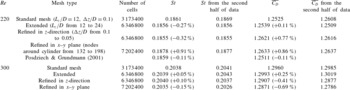
Results of the 3D mesh dependence study. The relative errors in the brackets are calculated by using the results obtained from the standard mesh as reference values.

The 3D mesh dependence study focused mainly on the mesh resolution and domain size in the spanwise direction. The 3D mesh formed using mesh 6 in table 2 is referred to as the standard 3D mesh in table 3. For the standard 3D mesh, the cell size in the spanwise direction
 $({\rm\Delta}z)$
is 0.1
 $D$
and the spanwise domain length is 12
 $D$
. Compared with the standard mesh, the mesh that is refined in the
 $z$
-direction has a spanwise cell size of 0.05
 $D$
, while the extended mesh has a spanwise domain length of 24
 $D$
. It should be noted that the spanwise domain length is specified to be an integer multiple of 4
 $D$
. The value 4
 $D$
is very close to the most unstable spanwise wavelength for mode A structure at
 $Re_{cr}$
obtained from linear stability analysis, e.g. 3.96
 $D$
by Barkley & Henderson (Reference Barkley and Henderson1996) and 3.966
 $D$
by Posdziech & Grundmann (Reference Posdziech and Grundmann2001). This is necessary for the accurate determination of the
 $Re_{cr}$
value in this paper. Furthermore, 3D simulations were also carried out with a mesh that was refined in the
 $x$
–
 $y$
plane. This mesh has the number of cells in both
 $x$
- and
 $y$
-directions 1.5 times that for the standard 3D mesh. Specifically, the number of cells around the cylinder is increased by 1.5 times, while the radial size of the first layer of mesh next to the cylinder is reduced by 1.5 times.
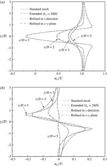
Averaged velocity profiles at a few streamwise locations in the near wake (
 $x/D=1$
, 2, 3 and 5) calculated with the four meshes listed in table 3 for
 $Re=300$
: (a) streamwise velocity profiles; (b) transverse velocity profiles.

The 3D mesh dependence study was carried out for
 $Re$
in both mode A (
 $Re=220$
) and mode B (
 $Re=300$
) regimes. It is found that a relatively long non-dimensional flow time (defined as
 $t^{\ast }=Ut/D$
) is required to achieve a fully developed 3D flow. After that, the calculation is continued for at least 1000 non-dimensional time units to obtain results that are in statistical equilibrium, where
 $St$
and
 $\overline{C_{D}}$
calculated from the second half of the sampling data are close enough to those determined from the whole sampling data sets (see table 3). For the 3D analysis,
 $St$
is determined using the peak frequency derived from the fast Fourier transform of the time history of the lift force coefficient. It is seen from table 3 that the two quantities obtained from the refined and extended meshes are very close to the ones obtained with the standard mesh (relative errors are within 1 %). In addition, figure 26 shows the streamwise and transverse velocity profiles at a few streamwise locations in the near wake (
 $x/D=1$
, 2, 3 and 5) calculated with the four meshes listed in table 3 for
 $Re=300$
. The velocity profiles are averaged over the same period of flow time (of more than 1000 non-dimensional time units) and over the cylinder span. It is seen in figure 26 that the differences of the averaged velocity profiles calculated with the four meshes listed in table 3 are negligibly small. The above results demonstrate that the standard mesh listed in table 3 is precise enough for the numerical simulations of the present study. Hence, the standard mesh is used in the 3D simulations in this study unless otherwise stated.
The present 3D DNS results have also been compared with independent spectral element method results reported in the literature. In the numerical study by Posdziech & Grundmann (Reference Posdziech and Grundmann2001) based on the spectral element method, a mesh dependence study was performed for flow past a circular cylinder at
 $Re=220$
, and converged
 $St$
and
 $\overline{C_{D}}$
values (table 3) were obtained when the polynomial order was larger than 10 and the number of Fourier modes was larger than 8. It is seen in table 3 that the results reported by Posdziech & Grundmann (Reference Posdziech and Grundmann2001) are extremely close to the present results based on the standard mesh.
It is worth noting that flow three-dimensionality in 3D DNS is normally triggered by small-scale numerical disturbance in the computational domain (e.g. by skewed mesh elements), in a similar way to the introduction of small-scale spanwise disturbance to the initial flow field (e.g. Henderson Reference Henderson1997; Thompson et al.
Reference Thompson, Leweke and Williamson2001) for the spectral element method to trigger flow three-dimensionality. In the present 3D DNS, the spanwise disturbance level observed in the computational domain is approximately
 $5\times 10^{-4}U$
for all of the 3D cases considered in this study (with
 $Re$
ranging from 100 to 300). Since the spanwise velocity beyond the secondary instability will grow to a much larger level (close to
 $U$
) after the flow is fully developed, the disturbance level introduced in the present study will not influence the simulation results noticeably.
The present DNS has been carried out with a Cray XC40 system supercomputer. For a typical 3D case with approximately 3.2 million cells, 360 processors have been used for parallel computation based on a scalability analysis. This leads to
 ${\sim}120$
h of wall-clock time for the numerical simulation of up to
 ${\sim}4000$
non-dimensional time units.