1. Introduction
Whatever definition of group selection one adopts there remain further questions about the proper description of the phenomenon so identified. By what kinds of models will we represent group selection, and by what procedures will such models be specified and identified given data measured on real populations? The issues are not independent—good models and good procedures for identifying them will depend on what we take them to be models of. But there is much to learn about useful definitions of group selection from the range of models available for representing group selection on any given definition. I briefly survey some proposals for representing group selection and correlative methods for specifying and identifying those models. The survey yields some lessons that illustrate a general principle about modeling complex causal systems. I’ll state the principle now; we’ll return to it toward the end of our survey: the state variables for a predictive or explanatory model of a complex causal system must be chosen so that when described by the state variables in the model, the system satisfies the Markov condition.Footnote 1
My concern here is with predictive rather than generative models. I have nothing to say about the usefulness or interest of models the point of which is to determine long-run equilibria for systems satisfying relevant formal constraints. I am rather concerned with models produced to describe the observed behavior of real populations, where such models are used either to explain the observed trajectory of a population or to predict its future behavior.
I begin with an assumption; it is defensible, but only at length. The assumption: whatever selection, and a fortiori group selection, may be, population genetics does not provide models that adequately represent such selection because such models are (almost) never causal models, while selection is a causal phenomenon. Some instances of the failure of population genetics to adequately model group selection will be surveyed here. Others won’t be. I take the failure of those models considered to represent the similar failure of their unconsidered fellows. In so doing I commit to an inference, the reliability of which I acknowledge to be uncertain.
2. Group Selection circa 1962
What counts as an appropriate model of group selection depends on how we define group selection. Group selection has sometimes been taken to be fully analogous to natural selection on individuals: group selection occurs when groups exhibit differential reproductive success, measured either by the number of daughter groups or the mean number of offspring among individual members of the group, where these differences are caused in part by group properties. Most of us were taught to think of group selection in something like this way. Some of us have given up this conception, but others haven’t, and even those who have find it hard to avoid all talk and all inferential practice in which this conception is implicit. We are inclined to approach questions about the level or unit of selection by asking ‘what entity benefits’, to attribute fitnesses to groups (or not), to wonder whether altruistic groups are reproducing faster than selfish individuals are invading, and so on.
But, from our causal perspective, any such definition of group selection is a bad idea because it does not precisely identify any phenomenon that is correctly explained only by models that appeal to the causal efficacy of the relevant group properties. Some instances of group selection so defined require models in which group properties appear as causes, while others don’t. Consider a population in which some individual phenotypic variable T is a cause of individual reproductive success r. Let us take groups as our units, measure those groups with respect to  $\overline{T}$, the mean value of T in the group, and let group reproductive success R be measured by
 $\overline{r}$, the mean value of r in the group. Then
 $\overline{T}$ is, really truly, a cause of R: intervene on
 $\overline{T}$ and you will thereby change the probability distribution over
 $\overline{r}={}_{\mathrm{df}\,}R$, for the group on which you have intervened. Matters are not interestingly different if we measure R by the number of daughter groups produced, so long as R depends on r. In either case, group selection, on our definition, occurs.
And yet pretty clearly we did not mean to include this kind of case as group selection. No information essential for either explanatory or predictive purposes is lost if we model this population at the level of individuals. The definition isn’t incoherent; it just doesn’t uniquely identify the phenomena of interest. Consequently, those employing anything very much like this conception of selection must immediately confront the issue of reduction—where can ‘group selection’ be reduced to individual selection, and where not?
3. Group Selection circa 1972
One might attempt to solve, or more exactly avoid, the reduction question by assessing the relative influence of group and individual properties on the change in mean phenotype. Initial efforts to do this proceeded by factoring the covariance between trait and the change in mean phenotype into two components: within and between group covariances. The standard procedure employs some version of Price's Equation. Here is one:

where  $\overline{w}$ is the mean absolute fitness in the population at generation g,
 $\Delta \overline{T}$ is the change in mean phenotype between generations g and
 $g+1$, i indexes individuals in groups, and j indexes groups.
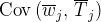 $\mathrm{Cov}\,( \overline{w}_{j},\,\overline{T}_{j}) $ is taken as a measure of group selection and
 $E( \mathrm{Cov}\,( w_{ij},\, T_{ij}) ) $ as a measure of individual selection (Price Reference Price1972; Wade Reference Wade1985; Sober and Wilson Reference Sober and Wilson1998).
The interpretation is suspect on its face. Covariance methods are unreliable when the dependent variable is a nonlinear function of the exogenous variables, and of course survival and reproductive success, being discrete, are nearly always nonlinear functions of their causes. Further, as a test for group selection, it is prone to false positives, since 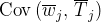 $\mathrm{Cov}\,( \overline{w}_{j},\,\overline{T}_{j}) $ can be nonzero even when group properties do not influence survival or reproductive success (see Okasha Reference Okasha2005 and references therein). Still, one might hope that when group selection is acting, the interpretation of Price's Equation offers a reasonably reliable method for approximating the relative influence of group and individual properties on the change in mean phenotype. The hope is misplaced.
Below I give the results of some agent-based simulations of selection. The models take the following form. There is no survival across generations, and no mortality within a generation. Individuals have 0, 1, 2, or 3 offspring, each with some probability given by

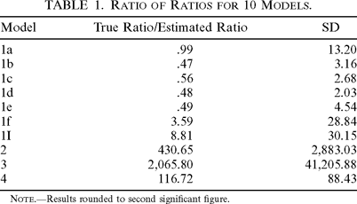
Variable T is the focal trait, and group selection is generated by the influence of Freq(T), measured as the frequency of T in the group to which an individual belongs. All variables other than Freq(T) are binary. Each model was run 100 times with an initial population size of 10,000, distributed randomly among 100 groups. The true strength of selection pressures on T, and Freq(T) was computed counterfactually by considering the expected change in the frequency of T in the population between successive generations and the expected change conditional on the relevant variable (T, Freq(T)) taking the value zero in all occurrences in Equation (2). I report in Table 1 the average of the absolute value of the ratio of the ratio of the strength of group to individual selection as assessed counterfactually to the ratio of strengths as estimated using Price's Equation. The details of each model and the computations used to generate the results are given in the Appendix.

| Model | True Ratio/Estimated Ratio | SD |
|---|---|---|
| 1a | .99 | 13.20 |
| 1b | .47 | 3.16 |
| 1c | .56 | 2.68 |
| 1d | .48 | 2.03 |
| 1e | .49 | 4.54 |
| 1f | 3.59 | 28.84 |
| 1I | 8.81 | 30.15 |
| 2 | 430.65 | 2,883.03 |
| 3 | 2,065.80 | 41,205.88 |
| 4 | 116.72 | 88.43 |
Note.—Results rounded to second significant figure.
The results do not come from a full Monte Carlo trial and so do not characterize the reliability of this use of Price's Equation, even for these models in particular. The simulation results suffice only to establish the conclusions drawn here. Sometimes Price's Equation gives a reasonably good approximation to the true relative influence. But in none of the models run are these estimates perfectly reliable; the estimates are wildly inaccurate in many of them, and the standard deviations are in no case reassuring. It is therefore often a locally bad idea to use Price's Equation in this way and a locally good idea only if one knows quite a bit about the causal structure governing the population. Its use in general to estimate the relative importance of group and individual selection is consequently a bad idea.
4. Group Selection circa 1987
A different set of methods for avoiding the reduction question employ regression rather than ANCOVA. Broadly known as contextual analysis (Heisler and Damuth Reference Heisler and Damuth1987; Goodnight, Schwartz, and Stevens Reference Goodnight, Schwartz and Stevens1992), these methods offer an expansion of the partition of covariances afforded by Price's Equation (Frank Reference Frank1997); the result of the expansion is a redefinition of group selection. The basic idea is to regress T and B(GP) on (some component of) fitness to produce a regression equation

where w is individual fitness, GP is some moment of the distribution of T in the group to which an individual belongs, and B(GP) is the individual property of belonging to a group characterized by GP.Footnote 2 The partial regression coefficients are then used as estimates of parameters in the equation

where  $\overline{w}$ and
 $\Delta \overline{T}$ are as before the mean fitness at generation g and change in mean phenotype between generations g and
 $g+1$, respectively. The first term is taken to measure the strength of individual selection on T, the second the strength of group selection on T.
The unit of analysis is, evidently, the individual, but group properties are represented in the regression equation by surrogates, namely, the property of belonging to a group having the property of interest (e.g., values of Freq(T) in Equation [2] above). It should be obvious from Equations (3) and (4) that contextual analysis presupposes a redefinition of group selection: group selection occurs if and only if the ‘belonging to’ variable (e.g., Freq(T)) causally influences survival or reproductive success (Goodnight et al. Reference Goodnight, Schwartz and Stevens1992; Okasha Reference Okasha2004).
Contextual analysis has distinct advantages. Most important among them is the fact that it represents aspects of the causal structure governing reproductive success insofar as the variables on the right-hand side of the regression Equation (3) are taken to be causes of fitness. It is worth pausing to explore one insight that arises immediately from such explicitness about causal structure, at least when linearity and additivity are not assumed.
Consider a model where the probability distribution over reproductive success follows an equation like Equation (2) above, either without migration or with random migration. Within any group, for otherwise identical individuals with, respectively,  $T=0$ and
 $T=1$, the difference in fitness is proportional to
 $\gamma \mathrm{Freq}\,( T) -\alpha $. If
 $\gamma \mathrm{Freq}\,( T) -\alpha $ is negative, then
 $T=1$ will increase in frequency in that group (e.g., when α and γ are both negative and
 $\mathrm{Freq}\,( T) > \alpha / \gamma $). Judged by conventional definitions,
 $T=1$ is not an altruistic trait, since individuals with
 $T=0$ would increase their fitness by switching to
 $T=1$ when they have a sufficiently high value of Freq(T). On the other hand, the frequency of
 $T=1$ may increases in these systems, and when it does, it does so only as a result of the influence of Freq(T) on reproductive success, that is, only as a result of group selection as redefined by contextual analysis. If traits like this are not to be considered altruistic, it is an important insight that some nonaltruistic traits require group selection if they are to evolve: traits like
 $T=1$ evolve only under group selection and, more particularly, only under group selection regimes with interactions between T and Freq(T).Footnote 3 The result is immediate when reproductive success is modeled causally without the assumption of linear dependencies; it is unobvious and painstaking to reproduce using traditional fitness based models.
A second advantage of contextual analysis is that it makes the issue of reduction completely trivial. The regression Equation (3) gives a perfectly innocuous reduction from the group to the individual level. But this reduction in no way threatens to obscure the crucial role of group properties in generating survival and reproductive success. That role is itself explicitly represented by the surrogate ‘belonging to’ variables in the regression equation. Sometimes the frequency of a trait in a group to which an individual belongs influences the survival and reproductive success of that individual, and the fact that this is so is not made to go away, even apparently, by the model employed to represent selection at the individual level.
Despite these advantages, contextual analysis, at least as commonly practiced, is a bad idea. First, linear regression is an unreliable procedure for model identification when the dependent variable is a nonlinear response to the independent variables. This is almost certain to be true of any wild population since both reproductive success and survival will be nonlinear functions of their immediate causes. Second, regression methods in general are demonstrably unreliable procedures for model selection. The most obvious failure involves unmeasured common causes. For example, if there is selection on a trait variable Z, and migration is assortative with  $T=1$ individuals differentially preferring groups with high
 $\overline{Z}$, then even when Freq(T) does not influence reproductive success, the regression coefficient for Freq(T) in Equation (3) will be nonzero.
Finally, Equation (4) is also problematic, because it reintroduces the very idea we were trying to avoid, namely, that group selection involves the differential reproductive success of groups. To see this, note that  $\mathrm{Cov}\,( T,\,\:\mathrm{Freq}\,( T) ) $ will be zero when migration is random and we correct for the mathematical fact that an individual's trait value for T influences Freq(T) by definition. Hence, following Equation (4), we will infer that group selection is not acting on the population. But that is clearly false and misleadingly so, when the causal structure involves interactions between traits and their frequencies—in such situations Freq(T) influences reproductive success, and it does so differently for individuals with
 $T=1$ and those with
 $T=0$. In fact, it is false and misleading even when no interaction term is present. The rate of change in mean phenotype depends on the relative difference in fitness between types. When Freq(T) positively influences expected reproductive success, relative differences in fitness will decrease as the influence of Freq(T) increases, even without an interaction term. Thus, even if the causal role of Freq(T) is immaterial for predicting equilibrium frequencies, it is nonetheless crucial for predicting the rate of change and hence the mean time until an equilibrium is reached.
5. Parameterizations and Predictive Competency
The predictive failures consequent to Equation (4) are, in some sense, invariant: so long as migration is random and Freq(T) causally influences reproductive success, Equation (4) will generate errors in the predicted time to equilibrium and sometimes in the predicted equilibrium frequencies themselves. This is not true of the errors implicit in the use of Equation (3) specifically or in regression methods in general. Errors will not be generated if a particular assumption holds true; this same assumption is also crucial to the predictive adequacy of a third way of modeling group selection, namely, the use of contextualized fitnesses in population genetics models. It is illuminating to treat contextualized fitnesses as one among at least three alternative ways to parameterize interactions.
Two such parameterizations are familiar from population ecology. The first we have already seen: one can, as in Equation (2), write the dependent variable as a nonadditive function of the independent variables. This is standard practice, for example, when estimating survival rates in mark-recapture studies with measured covariates. Differently, one can instead write the dependent as a distinct function of one independent variable for each value of the other, interactive, independent variable. This is standard practice in mark-recapture studies when sex is judged to influence the probability of survival. It is also implicit in time-lagged models of population growth, in which the lagged independent is used to induce ‘phase switching’ between years of increase and years of decrease. On this kind of parameterization, one takes the interactive variable to indirectly influence the dependent by determining the functional form of the dependence between the dependent variable and the remaining independent variables.
The second kind of parameterization makes possible the inclusion of several levels of ‘belonging to’ variables. Such multilevel models are given by a set of equations with the following general form:


Equation (5) writes the dependent Y as a function of n independent variables  $X_{1}{\mbox{--}} X_{n}$. Which function this is depends on the value of an interactive cause
 $X_{I}$, as expressed by Equation (6). But the mapping
 $g_{h}$ from
 $X_{I}$ values to the functions
 $f_{i}$ in turn depends on the value of a ‘higher level’ interactive cause
 $X_{H}$, with a dependence between
 $g_{h}$ and
 $X_{H}$ values expressed by the function k in Equation (7) (a nice review discussions of multilevel models in social scientific contexts can be found in Blalock Reference Blalock1984). Multilevel models are advantageous in that they permit a reduction of analytic level to that of chromosomes or even alleles, where the units of analysis are individual molecules. This need not obscure the causal role of ‘belonging to’ variables because, for example, the number of copies produced by a given molecule will be a function of its molecular properties, but which function will depend on the properties of the individual organism to which the molecule belongs, according to some second function, which itself will depend on the group or population to which the organism belongs, and so on. The disadvantage of multilevel models is that they complicate model selection and identification because they induce a more complex error structure (Diprete and Forristal Reference DiPrete and Forristal1994).
One might hope to avoid any explicit representation of the causal role of ‘belonging to’ variables by contextualizing fitnesses (cf. Kerr and Godfrey-Smith Reference Kerr and Godfrey-Smith2002). To do this one simply produces a fitness estimate for each class of units (alleles or individuals, whichever) where classes are individuated by the values of variables that covary with fitness. Dependencies between fitness and covariates are not expressly represented functionally, nor are interactions between these covariates, but both the dependencies and interactions are implicit in the fitness structure that results. The resulting population genetic models are prone to many of the same predictive failures that plague contextual analysis, and for the same reason. The causal structure relating covariates to one another and to reproductive success is not represented. Contextual analysis and population genetics models employing contextualized fitnesses are for this reason hostage to a crucial and frequently false assumption: the assumption that the associations between covariates and fitness will be remain stable.
6. Predictive Stability
If one uses data from some period  $t_{0}$ to
 $t_{1}$ to select and identify a model of a population and then projects that model by predicting behavior over the period
 $t_{1}{\mbox{--}} t_{2}$, one implicitly assumes that the associations between state variables and the predicted dependents remain unchanged between the period of observation and the projection period. That assumption can fail in a variety of ways.
The most obvious failure occurs when one intervenes on state variables before or during the projection period. If there are unmeasured common causes of dependent and independent state variables, the common causes will induce associations between dependent and independent variables that are modified by the intervention. Less obvious failures can be generated if one or more state variable is an interactive cause of a dependent. If the range of variation in an interactive cause differs between the observation period and the projection period, it may be that some ‘phase shifting’ thresholds are crossed in one but not the other period. Either results in predictive error when the interactive cause is not among the covariates included in the model.
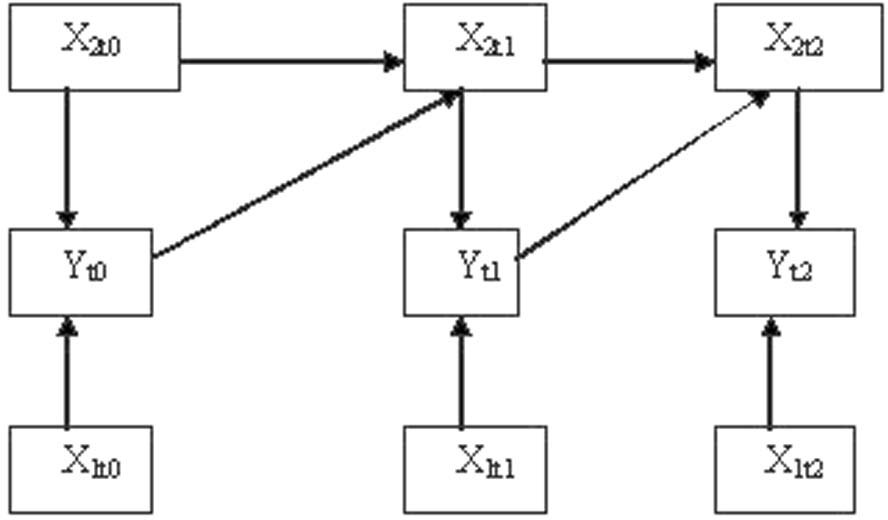
It turns out that there are sometimes good reasons to worry about exactly such situations. Consider a system like that in Figure 1 but modeled with time independent state variables Y and  $X_{1}$ (so
 $X_{2}$ is omitted from the mathematical model). The system so modeled will violate the Markov condition because the variable Y is a cause of its future value by way of a path that includes no state variable. This in itself induces predictive imprecision. Worse, if
 $X_{2}$ is an interactive cause of Y, so that the value of
 $X_{2}$ determines the functional relation between
 $X_{1}$ and Y, it may be that increases or decreases in Y during the projection period push
 $X_{2}$ over a threshold not crossed during the observation period, thereby inducing a bias in the model predictions.
Figure 1.

The frequencies of traits in groups may commonly be embedded in causal structures like that in Figure 1. Suppose, for individual organisms, both survival and reproductive success are effects of Freq(T), and offspring are differentially likely to remain in their natal groups. If Freq(T) at  $t_{1}$ influences Freq(T) at
 $t_{2}$ or later by some path that does not include survival or reproductive success at
 $t_{1}$, then the system will violate the Markov condition. For example, suppose Freq(T) influences immigration directly or indirectly through some environmental variable E, or suppose Freq(T) and E at
 $t_{1}$ both influence E at
 $t_{2}$, and E influences survival or reproductive success. Then the system will not be Markovian in models omitting both Freq(T) and E. If the relevant dependencies are interactive and unmodeled, this will generate both bias and imprecision in the model predictions.
Say that a causal system is complex if (a) the immediate causes of dependent variables are causally connected among themselves, (b) one or more of the causal connections is interactive, and (c) one or more variables is such that its current value is a cause of its future value. Say that a model is stable for a projection period if it can be reliably projected without re-estimation of model parameters for the projection period. Complex causal systems can be stably modeled only when the state variables are such that the system so modeled satisfies the Markov condition. Causal systems will violate the Markov condition and hence generate predictive errors, when they omit interactive causes that are themselves effects of state variables. Both contextual analysis and contextualized fitness models are likely to do this, for neither models the causal dependencies between and among the covariates used to predict fitness.
7. Conclusion
The causal structure governing survival and reproductive success is likely to be complex in many biological populations. Reproductive success can be reliably predicted in these populations only by models that explicitly represent this causal structure. If group properties influence reproductive success, and especially if they do so interactively, then surrogate ‘belonging to’ variables tracking these properties will have to be included in predictively competent models. It is interesting that standard population genetics models offer an explicitly causal role to only one state variable, and even then only in one special case: type frequencies are represented as causes of reproductive success in the special case of frequency- or density-dependent selection. It is ironic that this special case is also the limiting case of group selection: group selection acting on a population with only one group.
I now retract the assumption with which I began, namely, that population genetics models are bad models of selection. I tender it again, now not as an assumption but as a conclusion.
Appendix
All models were implemented in SAS. Individual reproductive success was determined at random with

for  $n=1$, 2, 3, and

Variables T, Z,  $E_{1}$ and
 $E_{2}$ are binary with values zero and one. Variables T and Z are perfectly heritable, with
 $\mathrm{Pr}\,( T=1) =.5$ and
 $\mathrm{Pr}\,( Z=1) =.7$ in the first generation. Variable
 $E_{1}$ varies among individuals and over generations, but not within generations, with
 $\mathrm{Pr}\,( E_{1}) =.4$ for each individual;
 $E_{2}$ varies among groups within a generation and over generations, but not within groups, with
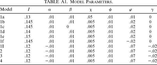
 $\mathrm{Pr}\,( E_{2}=1) =.6$ for each group at each generation. There is no survivorship. Model parameters are given in Table A1.
In all models there are 100 groups; individuals in the first generation are randomly assigned to a group. In models 1a–1I there was no migration. In model 2 migration is random at the beginning of each generation. In models 3 and 4 migration is structured. If N is the group number (0 to 99) of the parent, let  $L=N-1$,
 $R=N+1$,
 $A=N-10$, and
 $B=N+10$, except that if as so calculated
 $L< 0$, then
 $L=99$; if
 $R> 99$, then
 $R=0$; if
 $A< 0$, then
 $A=( N-10) +100$; and if
 $B> 99$, then
 $B=( N+10) -100$. In model 3, individuals are assigned to groups N, L, R, A, and B at random. In model 4 individuals are assigned to groups N, L, R, A, and B with probability

where POS ranges over N, L, R, A, and B, and frequencies are calculated at the parent's generation.
For each model 100 lineages were generated and run for 20 generations. Model statistics were calculated for generations 3–18 to reduce variation, and runs were terminated for the same reason if the population frequency of  $T=0$ became higher than .95 or lower than .05. The reliability of Price's Equation as an estimator of the relative influence of group and individual selection is assessed as follows. The expected change in mean population phenotype between two consecutive generations is
 $E( \Delta ( F( T) ) =( C( T) / n) ( 1-( \overline{w}_{T=1}/ \overline{w}) ) $, where F(T) is the frequency of
 $T=1$ in the population, C(T) is the count of individuals with
 $T=1$, n is the total population size,
 $\overline{w}_{T=1}$ is the mean fitness of individuals with
 $T=1$, and
 $\overline{w}$ is the mean fitness of the population. The effect of a selection pressure may then be calculated as the difference between this quantity and the change expected, counterfactually, were the relevant variable (T, Freq(T)) set to zero at every occurrence in Equation (2). Hence, the effect of group selection is given by

the effect of individual selection is given similarly, replacing set Freq( $T=0$) with set
 $T=0$:

The ratio of the effects may then be taken, yielding as the true relative effect of group selection to individual selection the quantity  $\mathrm{TREGS}\,=\mathrm{GS}\,/ \mathrm{IS}\,$. We may then take the ratio of this quantity to a similar ratio taken from Price's Equation:

where  $\overline{R}_{j}$ is the mean reproductive success in the jth group and
 $r_{ij}$ is the reproductive success of the ith member of the jth group. The figures reported in Table 1 are the mean over generations 3–18 of all lineages of the absolute value of the ratio of TREGS to PEREGS.

| Model | I | α | β | χ | φ | ϕ | γ |
|---|---|---|---|---|---|---|---|
| 1a | .13 | .01 | .01 | .05 | .01 | .01 | 0 |
| 1b | .145 | .01 | .01 | .005 | .01 | .02 | 0 |
| 1c | .145 | .01 | 0 | .005 | .01 | .02 | 0 |
| 1d | .14 | .01 | .01 | .005 | .01 | .02 | 0 |
| 1e | .15 | .01 | .01 | .005 | .01 | .02 | 0 |
| 1f | .145 | .01 | .01 | .005 | .01 | −.02 | 0 |
| 1I | .12 | −.01 | .01 | .005 | .01 | .07 | −.02 |
| 2 | .12 | −.01 | .01 | .005 | .01 | .07 | −.02 |
| 3 | .12 | −.01 | .01 | .005 | .01 | .07 | −.02 |
| 4 | .12 | −.01 | .01 | .005 | .01 | .07 | −.02 |