
1. Introduction
Bypass transition has been well observed and studied in turbomachinery owing to its significant impacts on the performance of the machine. The term ‘bypass transition’ is used for all transition processes that bypass the classic transition route via the exponential growth of Tollmien–Schlichting (TS) waves. There have been enormous studies on the onset of bypass transition, mostly induced by free-stream turbulence (see e.g. Jacobs & Durbin (Reference Jacobs and Durbin2001), Matsubara & Alfredsson (Reference Matsubara and Alfredsson2001), Brandt, Schlatter & Henningson (Reference Brandt, Schlatter and Henningson2004) and Fransson, Matsubara & Alfredsson (Reference Fransson, Matsubara and Alfredsson2005) to name but a few). Bypass transition can also develop in the presence of surface elements, which has been widely investigated experimentally (Gaster, Grosch & Jackson Reference Gaster, Grosch and Jackson1994; White Reference White2002; Downs, White & Denissen Reference Downs, White and Denissen2008) and numerically (De Tullio et al. Reference De Tullio, Paredes, Sandham and Theofilis2013; Goldstein, Chu & Brown Reference Goldstein, Chu and Brown2017; Bucci et al. Reference Bucci, Puckert, Andriano, Loiseau, Cherubini, Robinet and Rist2018). In this work, we study numerically the flow development downstream of a pair of streamwise-aligned plasma actuators analogous to roughness elements and focus on the bypass transition when the actuators are sufficiently long.
1.1. Bypass transition
The early stage of bypass transition involves the formation of streaks due to the lift-up of the mean momentum (Taylor Reference Taylor1939; Landahl Reference Landahl1975). The low-momentum (high-momentum) fluid is displaced upwards (downwards) by a small positive (negative) wall-normal velocity disturbance, leading to high- and low-speed streaks. When the boundary layer is subject to free-stream turbulence, streaks are formed as a result of the low-frequency disturbances entering the boundary layer via shear sheltering (Hunt & Durbin Reference Hunt and Durbin1999) and then tilting the base shear via the lift-up (Landahl Reference Landahl1980). Using linear optimal disturbance analysis, it has been found that the optimal inflow condition leading to the maximum transient energy growth downstream is a pair of steady streamwise-aligned vortices, resulting in a pair of streamwise velocity streaks (Butler & Farrell Reference Butler and Farrell1992; Andersson, Berggren & Henningson Reference Andersson, Berggren and Henningson1999; Monokrousos et al. Reference Monokrousos, Åkervik, Brandt and Henningson2010).
After generation, the streaks are further amplified as they are convected downstream. It was reported that the amplitude of the streaks increases as the square root of the distance from the leading edge (Kendall Reference Kendall1985). The streaks interact with the streamwise vorticity and the high-speed (low-speed) streaks are lifted towards (away from) the wall via a nonlinear lift-up mechanism, leaving an inflection point in the mean shear profile that is prone to secondary instabilities (Mao et al. Reference Mao, Zaki, Blackburn and Sherwin2017). Swearingen & Blackwelder (Reference Swearingen and Blackwelder1987) first identified two forms of secondary instability leading to the breakdown of streaks in Görtler flow: a sinuous type and a varicose type. The sinuous mode is associated with the spanwise inflectional velocity profile and features an asymmetric pattern with respect to the unstable streak, whereas the varicose one is related to the wall-normal inflection point and presents a symmetric pattern. The sinuous instability usually occurs around the low-speed streak that is lifted upwards and varicose instability is found in the overlapping region between the high- and low-speed streaks (Vaughan & Zaki Reference Vaughan and Zaki2011; Hack & Zaki Reference Hack and Zaki2014). Andersson et al. (Reference Andersson, Brandt, Bottaro and Henningson2001) performed inviscid instability analysis on optimal streaks and found that the critical streak amplitudes are  $26\,\%$ and
 $37\,\%$ for the sinuous and varicose instabilities, respectively. More recently, Puckert & Rist (Reference Puckert and Rist2019) observed in experiments that the sinuous and varicose modes coexist in the wake of a roughness element and the two modes are coupled with frequency lock-in.
The development of streak instabilities results in either turbulent spots or turbulent wedges, which eventually lead to transition to turbulence. A turbulent spot is commonly found in boundary layer flow subject to free-stream turbulence. A turbulent wedge, on the other hand, is a turbulent region bounded by a transitional region that develops in the spanwise direction as it propagates downstream (Schubauer & Klebanoff Reference Schubauer and Klebanoff1955). The turbulent wedge is generally found in roughness-induced bypass transition and is reported to spread laterally at a half-angle of  ${\sim }6^{\circ }$ (Zhong, Chong & Hodson Reference Zhong, Chong and Hodson2003; Goldstein et al. Reference Goldstein, Chu and Brown2017).
1.2. Plasma actuators
Dielectric-barrier-discharge (DBD) plasma actuators are electric devices that introduce the fluid flow by coupling the momentum. When the actuation is applied with a large AC voltage, the fluid near the surface is ionised and the charged particles are accelerated by the electric field. In this way the plasma actuators introduce momentum via collision between the charged particles and the ambient fluid (Boeuf et al. Reference Boeuf, Lagmich, Unfer and Pitchford2007), which can be modelled as an electrohydrodynamic (EHD) body force that produces a jet flow up to  $10\ \textrm {m}\ \textrm {s}^{-1}$ (Moreau Reference Moreau2007). When the plasma actuators are placed along the streamwise direction in a boundary layer, a body force in the spanwise direction is generated that results in a spanwise-directed wall jet. Jukes & Choi (Reference Jukes and Choi2013) found that the interaction between this wall jet and the oncoming boundary layer leads to the formation of a coherent streamwise vortex. More recently, Choi & Kim (Reference Choi and Kim2018) performed experiments on ring-type plasma actuators, which act as virtual roughness elements, and found that the body force leads to a wall-normal jet. In flow control, the body force induced by the DBD plasma actuators have been used for the delay of classic (Grundmann & Tropea Reference Grundmann and Tropea2008; Riherd & Roy Reference Riherd and Roy2013; Duchmann, Grundmann & Tropea Reference Duchmann, Grundmann and Tropea2014) and bypass (Hanson et al. Reference Hanson, Lavoie, Naguib and Morrison2010; Riherd & Roy Reference Riherd and Roy2014; Bade et al. Reference Bade, Hanson, Belson, Naguib, Lavoie and Rowley2016) transition, the suppression of flow separation (Schatzman & Thomas Reference Schatzman and Thomas2010; Walker & Segawa Reference Walker and Segawa2012; De Giorgi et al. Reference De Giorgi, Ficarella, Marra and Pescini2017), drag reduction (Wilkinson Reference Wilkinson2003; Choi, Jukes & Whalley Reference Choi, Jukes and Whalley2011) and lift enhancement (Little et al. Reference Little, Nishinara, Adamovich and Samimy2010; Feng et al. Reference Feng, Jukes, Choi and Wang2012; Greenbelt, Schneider & Schule Reference Greenbelt, Schneider and Schule2012).
The numerical simulation of DBD plasma actuators has been extensively studied, as it allows detailed examination of the induced flow. In these works, the model of DBD plasma actuators can be divided into two groups: simplified phenomenological models and first-principles-based models (Mahfoze & Laizet Reference Mahfoze and Laizet2017). Simplified models assume that the response of fluid flow and the formation of plasma are decoupled due to large differences in the characteristic velocities associated with each process (Mertz & Corke Reference Mertz and Corke2011). Popular simplified phenomenological models include the Shyy model (Shyy, Jayaraman & Andersson Reference Shyy, Jayaraman and Andersson2002) and the Suzen & Huang model (Suzen et al. Reference Suzen, Huang, Jacob and Ashpis2005). On the other hand, first-principles-based models aim to model the physical mechanisms of the plasma actuator and thus provide better accuracy (Nishida, Nonomura & Abe Reference Nishida, Nonomura and Abe2014; Dufour & Rogier Reference Dufour and Rogier2015). Consequently, transport equations for both the charged and neutral species as well as a Poisson equation for the electric field are solved to obtain the EHD body force, as will be adopted in the present work.
This paper is organised as follows. In § 2, the numerical method, including the plasma model, is introduced. In § 3, the problem description and computational set-up are presented. The results are reported in § 4. First, the plasma body force in the boundary layer is displayed in § 4.1, followed by a presentation of the wake flow downstream of the actuators in § 4.2. Then parametric study is performed and analysed in § 4.3, and finally the secondary instability and Orr mechanism observed during the breakdown of plasma-induced bypass transition are investigated in §§ 4.4 and 4.5, respectively. In § 5, biglobal stability and transient growth analysis are performed to further examine the mechanism of transition revealed in direct numerical simulations (DNS). In § 6, the main observations are summarised.
2. Numerical scheme
Plasma actuation in incompressible boundary layer flow over a flat plate is considered in this work. The flow is governed by the Navier–Stokes (NS) equations:
 \begin{equation} \partial_t\boldsymbol{u} + \boldsymbol{u} \boldsymbol{\cdot} \boldsymbol{\nabla} \boldsymbol{u} +\boldsymbol{\nabla} p - Re^{{-}1}\nabla^2\boldsymbol{u}+\boldsymbol{F}=0, \quad \boldsymbol{\nabla} \boldsymbol{\cdot} \boldsymbol{u}=0. \end{equation}
Here  $\boldsymbol {u}=(u, v, w)^\textrm {T}$,
 $p$ and
 $\boldsymbol {F}$, respectively, denote the non-dimensional velocity, pressure and external force induced by the plasma actuation;
 $u$,
 $v$ and
 $w$ are the streamwise, wall-normal and spanwise velocity components, respectively; and
 $Re$ is the Reynolds number, defined as
 $Re=U_{\infty }R/\nu$, where
 $\nu$ is the kinematic viscosity,
 $U_{\infty }$ is the free-stream velocity and
 $R$ is the half-thickness of the flat plate, which are used as the reference velocity and length, respectively. The velocity vector can be decomposed as
 \begin{equation} \boldsymbol{u}= \overline{\boldsymbol{U}}+ \boldsymbol{u}'', \end{equation}
where  $\boldsymbol {u}''$ is the velocity fluctuation and
 $\overline {\boldsymbol {U}}$ is the mean flow. The latter can be further decomposed as
 \begin{equation} \overline{\boldsymbol{U}}=\boldsymbol{U}+ \boldsymbol{u}', \end{equation}
where  $\boldsymbol {U}$ is the two-dimensional base flow when the plasma is not activated, satisfying (2.1a,b) when
 $\boldsymbol {F}=0$, and
 $\boldsymbol {u}'$ represents the mean disturbance induced by the plasma force. Just for clarity, in the rest of this paper,
 $\boldsymbol {u}'+\boldsymbol {u}''$ is referred to as total perturbation or disturbance and
 $\boldsymbol {u}''$ is referred to as perturbation or disturbance.
The force  $\boldsymbol {F}$ in (2.1a,b) is a force representing the cycle-averaged EHD force
 $\boldsymbol {F}_{EHD}$,
 \begin{equation} \boldsymbol{F}_{EHD}=\sum_{i}n_iq_i \boldsymbol{E}, \end{equation}
where  $n_i$ and
 $q_i$ are the density and charge of the
 $i$th species composing the plasma, respectively, and
 $\boldsymbol {E}$ denotes the electric field. The integration of
 $\boldsymbol {F}_{EHD}$ results in a steady force
 $\boldsymbol {F} = (1/\tau ) \int _0^\tau \boldsymbol {F}_{EHD}\,\textrm {d}t$ and the time variation of
 $\boldsymbol {F}_{EHD}$ is not considered in (2.1a,b). This simplification is due to the large gap between the time scales of the plasma dynamics and the fluid dynamics. A four-species plasma–fluid model (Dufour & Rogier Reference Dufour and Rogier2015), which solves the fluid equations for four species, is used to model the discharge mechanics of the DBD plasma actuators. To simulate the dynamics of each species, the conservation equations for their densities are considered,
 \begin{equation} \partial_i n_i + \boldsymbol{\nabla} \boldsymbol{\cdot} (n_i \boldsymbol{v}_i ) = S_i, \end{equation}
where  $\boldsymbol {v}_i$ is the velocity of the
 $i$th species. The last term
 $S_i$ represents the source term accounting for the creation of the charged species due to chemical reactions. The chemical reactions, describing the interaction between the electrons and the positive, negative and neutral particles, include ionisation, attachment, and electron–ion and ion–ion recombination. The rate coefficients for these reactions are obtained using the BOLSIG
 $+$ (Hagelaar & Pitchford Reference Hagelaar and Pitchford2005) and the LXCat databases (Phelps Reference Phelps2012; Pitchford & Boeuf Reference Pitchford and Boeuf2012). Neglecting the magnetic and inertial terms of the momentum equation, the velocity of the species can be obtained as
 \begin{equation} \boldsymbol{v}_i = \mu_i \boldsymbol{E} + D_i \frac{\boldsymbol{\nabla} n_i}{n_i}, \end{equation}
where  $\mu _i$ and
 $D_i$ are the mobility and diffusion coefficients, respectively, of the corresponding species.
The electric field  $\boldsymbol {E}$ is obtained by solving a Poisson equation for the electric potential
 $\phi$, namely
 \begin{equation} \boldsymbol{\nabla} \boldsymbol{\cdot} (\epsilon \boldsymbol{\nabla} \phi ) = \sum_{i} n_i q_i \quad \mathrm{and} \quad \boldsymbol{E} ={-}\boldsymbol{\nabla} \phi, \end{equation}
where  $\epsilon$ is the local material permittivity.
3. Problem description and computational domain
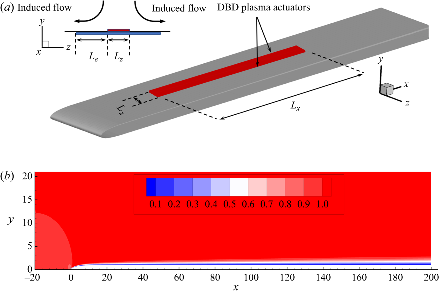
A schematic diagram of the geometry of a flat plate with a slender leading edge is shown in figure 1(a). The computational domain spans from  $x=-20$ to
 $x=200$ in the streamwise direction, and from
 $y=-40$ to
 $y=40$ in the wall-normal direction. The leading edge is located at
 $x=0$ with an elliptic shape and aspect ratio
 $AR=20$.
(a) Schematics of plasma actuators on the flat plate. (b) Contour of the streamwise velocity component of the base flow around the upper part of the flat plate at  $Re=800$, which will be used in all the following studies.

As aforementioned, the steady two-dimensional base flow  $\boldsymbol {U}$ is obtained by integrating the full nonlinear NS equations (2.1a,b) with
 $\boldsymbol {F}=0$ until a steady solution is reached. Figure 1(b) shows the base flow profile over the upper part of the flat plate at
 $Re=800$, which will be used in all the rest of this work. Downstream of the leading edge, the flow develops into a zero-pressure-gradient boundary layer and the boundary layer thickness is approximately
 $\delta =1.8$ at the end of the computational domain. The shape factor is computed at various locations downstream of the leading edge and is always around
 $2.52$. Validation of the simulation can be found in Wang, Mao & Zaki (Reference Wang, Mao and Zaki2019).
The numerical code used here has been extensively validated in previous works for various flow problems, such as a backward-facing step (Barkley, Blackburn & Sherwin Reference Barkley, Blackburn and Sherwin2008; Mao Reference Mao2015), a flat plate with a leading edge (Wang et al. Reference Wang, Mao and Zaki2019; Huang et al. Reference Huang, Xiao, Ren, Wang, Xi and Mao2021), etc. The governing equations are discretised in the  $x\text {--}y$ plane using the spectral element method into
 $2505$ elements, most of which are clustered around the upper side of the plate where the plasma actuation and bypass transition will be investigated. Each element is further decomposed into a
 $(\mathcal {P}+1)\times (\mathcal {P}+1)$ grid, where
 $\mathcal {P}$ is the polynomial order that defines the resolution. In this work,
 $\mathcal {P}=8$ is adopted, i.e. the spatial order of discretisation is
 $8$. In the spanwise direction, the flow variables are decomposed as
 \begin{equation} \boldsymbol{u}(x,y,z) = \sum_{n=0}^{n_z} \boldsymbol{u}_{\beta}(x,y)\textrm{e}^{\textrm{i}\beta z}, \end{equation}
where a total of  $n_z=192$ Fourier modes over the spanwise width of the domain
 $12$ are computed. Moreover, the temporal order of discretisation is set to
 $2$. Detailed descriptions of the boundary conditions can be found in Wang et al. (Reference Wang, Mao and Zaki2019) and Huang et al. (Reference Huang, Xiao, Ren, Wang, Xi and Mao2021).
The two-dimensional EHD force distribution of a single plasma actuator is computed separately in a dimensional setting by the four-species plasma–fluid model described in § 2. The thicknesses of the upper/lower electrodes and the dielectric sheet are  $50\ \mathrm {\mu } \textrm {m}$ and
 $150\ \mathrm {\mu } \textrm {m}$, respectively. The distance between the upper and lower electrode edges is
 $L_e=1\ \textrm {mm}$, as indicated in figure 1(a). The AC voltage applied to the plasma actuators is sinusoidal, with an amplitude of
 $2 \ \textrm {kV}$, and three frequencies,
 $f=20$,
 $40$ and
 $60\ \textrm {kHz}$, are considered. The computational domain contains 58 795 elements, of which 46 136 are in the fluid domain. The two-dimensional force distribution is non-dimensionalised using the density (
 $1.225\ \textrm {kg}\ \textrm {m}^{-3}$) and viscosity (
 $1.81\times 10^{-5}\ \textrm {kg}\ \textrm {m}^{-1} \ \textrm {s}^{-1}$) of air before application to the three-dimensional boundary layer. This model and its numerical discretisation have been validated in various configurations for atmospheric-pressure plasma discharges (Kourtzanidis, Dufour & Rogier Reference Kourtzanidis, Dufour and Rogier2020a,Reference Kourtzanidis, Dufour and Rogierb).
The arrangement of the DBD plasma actuators on the plate is shown in figure 1(a). Plasma actuators with different lengths of the upper electrode are tested and it is found that the force topology remains the same as long as  $L_e$ is fixed over the parameters considered in this work. The actuators generate a jet-like velocity in the spanwise direction. This leads to a wall-ward velocity component above the actuators because fluid is brought towards the actuator from above to replace that drawn away laterally by the EHD body force (Jukes & Choi Reference Jukes and Choi2013). The upstream edge of the plasma actuators is located at
 $x=30$, where the Reynolds number based on boundary layer thickness at this location is
 $Re_{\delta }=560$. Different streamwise lengths of the plasma actuator ranging from
 $L_x=10$ to
 $L_x=90$ are investigated. The two plasma actuators are placed with respect to the centre position of the domain
 $z=6$, and spanwise distances of the upper electrode
 $L_z$ ranging from
 $0.1$ to
 $1.5$ are considered.
4. Plasma-induced transition
4.1. Plasma-induced body forcing
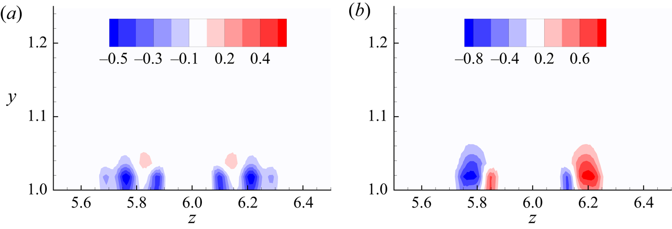
Figure 2 shows the distribution of the wall-normal and spanwise components of the EHD force exerted by the plasma actuators at  $60 \ \textrm {kHz}$, denoted as
 $F_y$ and
 $F_z$, respectively. The plasma actuators are arranged to produce vertical velocity towards the wall as seen in figure 1(a). In figure 1(b), the spanwise component on each side has two opposing regions, which is due to the push–pull scenario of the AC cycle (Thomas, Enloe & Wilkinson Reference Thomas, Enloe and Wilkinson2010). The larger force region dominates and leads to an outward jet from the centre. A separate simulation of the plasma force in quiescent air is performed in order to examine the effect of the actuator. The momentum coefficient (Jukes & Choi Reference Jukes and Choi2012) computed at
 $z=6.65$, where the spanwise velocity reaches its maximum value, is around
 $0.018\,\%$. Note that the minor difference in the two opposing force distributions is due to linear interpolation of the force when applied to the boundary layer flow domain. The force reaches
 $y=1.08$, while the edge of the boundary layer at the upstream edge of the actuator is at about
 $y=1.7$.
Contours of (a) wall-normal and (b) spanwise components of the EHD force distribution at  $60\ \textrm {kHz}$ and
 $2\ \textrm {kV}$, which will be used in all the following if not otherwise stated.

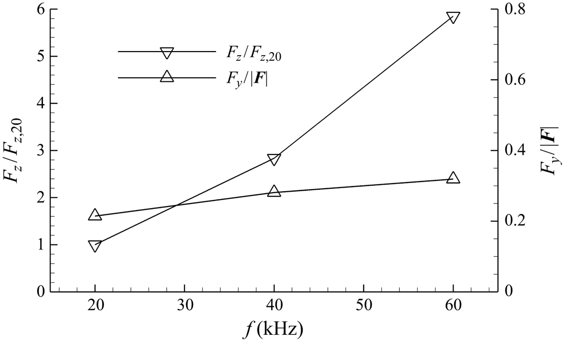
The effect of actuation frequency on the generated EHD force is shown in figure 3. As the frequency is increased from  $20\ \textrm {kHz}$ to
 $60\ \textrm {kHz}$, the variation in the resultant force direction is less than
 $8^{\circ }$. On the other hand, the magnitude of the spanwise component of the force increases with the frequency. This suggests that the plasma actuators are capable of inducing body force of a wide range of strength, whilst maintaining a relatively consistent force distribution and direction. In the rest of this work, the frequency is set to
 $60\ \textrm {kHz}$ unless otherwise stated. The frequency corresponds to a non-dimensionalised value of around
 $31.4$, which is two orders higher than the high-frequency disturbance mode (0.32–0.64) used to trigger bypass transition in a flat-plate boundary layer flow in Zaki & Durbin (Reference Zaki and Durbin2005).
Comparison of the EHD force obtained at different frequency  $f$. The left
 $y$-axis shows the magnitude of
 $F_{z}$ scaled by
 $F_{z,20}$ (at
 $20\ \textrm {kHz}$); the right
 $y$-axis shows the ratio between
 $F_y$ and the magnitude of the resultant force
 $\vert \boldsymbol {F} \vert$ at each frequency. All the forces are obtained by integration over the
 $y\text {--}z$ plane.

4.2. Wake flow of plasma actuators
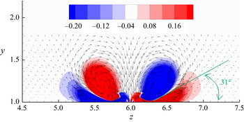
DNS of boundary layer flow with plasma actuation are performed. A pair of plasma actuators is placed over a flat plate in such a way that the plasma wall jets are induced away from each other, while creating an entrained flow towards the wall between the two actuators. This leads to the formation of a pair of counter-rotating vortices, as shown in figure 4. Similar phenomena were observed in experimental studies (Jukes et al. Reference Jukes, Choi, Segawa and Yoshida2008). Jukes & Choi (Reference Jukes and Choi2013) further suggested that the spanwise-directed wall jet interacts with the oncoming boundary layer, and streamwise vortices are created as a result. In figure 4, secondary vorticity is induced below the primary vortices, which is due to the preservation of the no-slip wall boundary condition. Whalley & Choi (Reference Whalley and Choi2013) experimentally investigated DBD plasma actuators in quiescent air and reported that the secondary vorticity wraps around the starting vortex and steers its trajectory away from the wall at an angle of  $31^{\circ }$, which agrees well with the present observation shown in figure 4.
Contour of streamwise vorticity induced by the plasma actuators. The direction and length of the arrows indicate the direction and magnitude of the induced velocity.

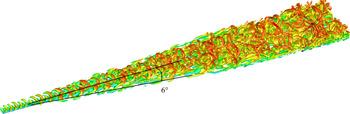
The wake flow downstream of the actuators with  $(L_x, L_z)=(90,0.25)$ is shown in figure 5. It is clear that the transition downstream of the plasma actuators occurs through a turbulent wedge, which is often found in turbulent flow developed in the presence of surface elements, in contrast to turbulent spots induced by free-stream disturbance. The spreading half-angle is approximately
 $6^{\circ }$, in agreement with those reported in the literature. For example, Zhong et al. (Reference Zhong, Chong and Hodson2003) observed in experiment a spreading half-angle of
 $6.5^{\circ }$ of turbulent wedge induced by a three-dimensional surface roughness in a laminar boundary layer flow. Goldstein et al. (Reference Goldstein, Chu and Brown2017) found a turbulent wedge spreading half-angle of
 $6^{\circ }$ developed downstream of an asymmetric cylindrical perturbation in their numerical simulations. The spreading half-angles for other settings of
 $(L_x, L_z)$ are all around
 $6^{\circ }$ and not displayed here for brevity.
Turbulent wedge and vortical structure with  $(L_x, L_z)=(90,0.25)$, visualised with an isosurface of
 $\lambda _2=-0.01$ and coloured by instantaneous streamwise velocity
 $u$.

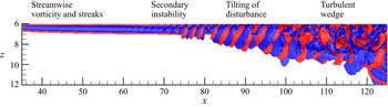
We divide the transition process induced by plasma actuation into four stages, which is demonstrated in figure 6 using the isosurfaces of streamwise vorticity. In the first stage, vortical disturbance is generated by the plasma actuators as discussed previously. Once the pair of counter-rotating vortices is created, it is continuously supplied with streamwise vorticity from the outer layer of the spanwise jet induced by the plasma to increase the circulation (Jukes & Choi Reference Jukes and Choi2013). As a consequence, streaks are generated due to lift-up and amplified along the streamwise direction.
Isosurfaces of streamwise vorticity 0.1 (red) and  $-0.1$ (blue) with
 $(L_x, L_z)=(90,0.25)$. The plot shows half of the domain in the spanwise direction, which is scaled by 2.5. The four stages of the transition process are indicated at corresponding locations.

As the amplitude of the disturbance grows beyond a threshold, secondary instability occurs in the second stage. In figure 6 positive/negative tilted streamwise vorticity starts to appear at  $x=70$. Similar observations were made by Goldstein et al. (Reference Goldstein, Chu and Brown2017) and Saikishan, Goldstein & Brown (Reference Saikishan, Goldstein and Brown2019) along the edge of flow developed downstream of a roughness element, and the patterns were named as tilted ‘pancakes’ of
 $\omega _x$. From a vorticity point of view, the tilted ‘pancakes’ are a signature of the vorticity tilting process turning
 $\omega _z$ into
 $\omega _x$ and
 $\omega _y$ (Goldstein et al. Reference Goldstein, Chu and Brown2017). Starting from
 $x=82$, there is a clear expansion of the vorticity in the spanwise direction. In this stage, the shape of the disturbances is further tilted by the spanwise shear and will be elaborated later. In the final stage, a turbulent wedge is formed and the flow becomes turbulent. Details of the secondary instability and its further tilting by the shear will be discussed in the following sections.
4.3. Parametric study
In this section, the effects of  $L_x$,
 $L_z$ and
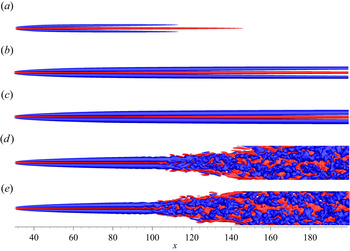
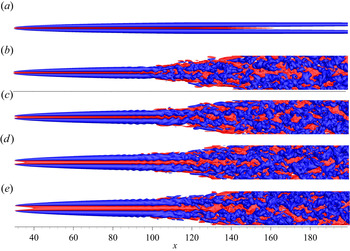
 $f$ on the flow development are presented. Figure 7 shows the total streamwise perturbation
 $u'+u''$ with
 $L_z=0.25$ and
 $L_x$ ranging from
 $10$ to
 $90$. A high-speed streak can be seen in the centre, with two low-speed streaks on each side. Similar results are found in the experimental work of Gouder et al. (Reference Gouder, Naguib, Lavoie and Morrison2017), where a pair of plasma actuators, arranged in the same way as in the current work, were used to control boundary layer streaks. In contrast, a single roughness element induces a wake that consists of a central low-speed streak, surrounded by a pair of high- and low-speed ones on each side (Loiseau et al. Reference Loiseau, Robinet, Cherubini and Leriche2014). The streaks in figure 7(a) grow initially, and then decay and vanish completely. For larger values of
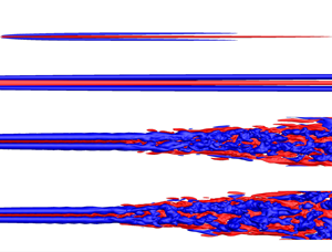
 $L_x$, the streaks become stronger and decay downstream of the actuators as seen in figure 7(b,c). In figure 7(d,e), the streaks are strong enough to break down and the flow becomes turbulent.
Isosurfaces of the total streamwise perturbation velocity  $u'+u''=0.1$ (red) and
 $u'+u''=-0.1$ (blue) for
 $L_z=0.25$ and various
 $L_x$: (a)
 $L_x=10$, (b)
 $L_x=30$, (c)
 $L_x=50$, (d)
 $L_x=70$ and (e)
 $L_x=90$.

We further investigate the effect of  $L_x$ quantitatively by examining the streak amplitude
 $A$ (Cossu & Brandt Reference Cossu and Brandt2002; Biancofiore, Brandt & Zaki Reference Biancofiore, Brandt and Zaki2017; Wang et al. Reference Wang, Mao and Zaki2019) defined as
 \begin{equation} A=\tfrac{1}{2} [\max(u-U) - \min(u-U) ]. \end{equation}
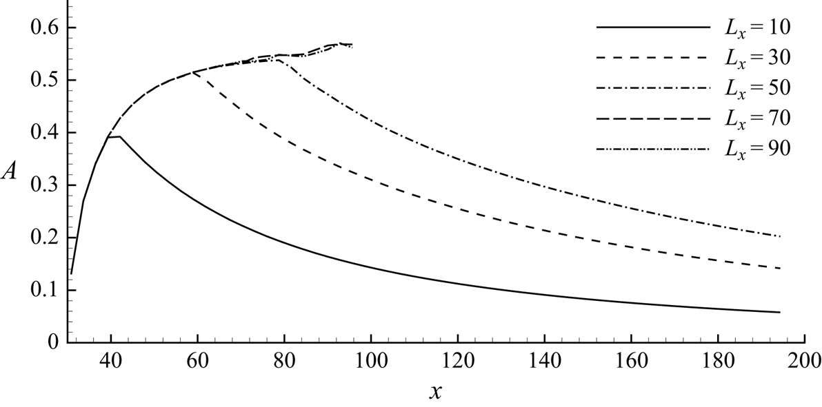
Figure 8 presents the streak amplitude  $A$ as a function of the streamwise location
 $x$ for each case in figure 7. For
 $L_x=70$ and
 $L_x=90$,
 $A$ in the turbulent regime is not shown as it is ill-defined and does not indicate the magnitude of streaks there. It can be seen that the streak amplitude increases at almost the same rate for all the cases. For the first three steady cases,
 $A$ starts to decrease immediately beyond the actuation region with a similar decay rate. These are in agreement with the experimental results in Jukes & Choi (Reference Jukes and Choi2013), where they investigated three different lengths of plasma actuators and reported that the vortex circulation increases along the length of the plasma actuators. They also observed that the strength of the vortex starts to decrease due to the viscous effect beyond the plasma region. For the three lengths that Jukes & Choi (Reference Jukes and Choi2013) tested, the vortex strength increases with the plasma length, from which they concluded that longer and stronger vortices can be generated by increasing the length of the actuators. In figure 8, the streak amplitude initially increases almost linearly before
 $x=40$ and then the growth rate gradually decreases until the peak is reached at around
 $x=80$. The streaks induced by plasma actuators, similar to those triggered by surface roughness, are stationary and do not demonstrate randomness, in contrast to those caused by free-stream turbulence (von Deyn et al. Reference von Deyn, Forooghi, Frohnapfel, Schlatter, Hanifi and Henningson2020). For cases where the length of plasma actuators exceeds the peak, the streak amplitude becomes large enough and the flow breaks down into turbulence. Similar bypass transition has been observed downstream of roughness elements with large enough size (von Deyn et al. Reference von Deyn, Forooghi, Frohnapfel, Schlatter, Hanifi and Henningson2020). Moreover, it can be expected that the breakdown location will remain approximately the same at even larger
 $L_x$.
Variation of the streak amplitude  $A$ along the streamwise direction at various values of
 $L_x$ and
 $L_z=0.25$.

Figure 9 presents the flow responses for  $L_x=90$ and
 $L_z$ varying from
 $0.1$ to
 $1.5$. Instability starts to appear at around
 $x=90$ and the streaks break down to turbulent flow for all cases except the first one. Two types of flow pattern can be observed: in figure 9(b), the positive streak undergoes asymmetric meandering motion with respect to
 $z=6$ (the centreline) prior to the breakdown, while in figure 9(d,e), the disturbances present a symmetric pattern. This difference will be discussed later.
Isosurfaces of the total streamwise perturbation velocity  $u'+u''=0.1$ (red) and
 $u'+u''=-0.1$ (blue) for
 $L_x=90$ and varying
 $L_z$: (a)
 $L_z=0.1$, (b)
 $L_z=0.25$, (c)
 $L_z=0.5$, (d)
 $L_z=1$ and (e)
 $L_z=1.5$.

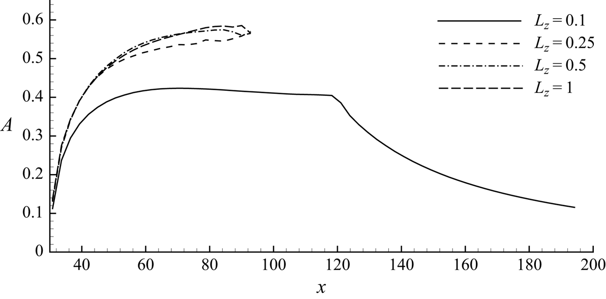
The effect of  $L_z$ on the streak amplitude is illustrated in figure 10. Similar to before,
 $A$ in the turbulent region is ill-defined by (4.1) and is not shown. For
 $L_z=0.1$ the streak amplitude reaches a peak value of
 $0.4$ and becomes almost flat after
 $x=60$. This is in agreement with the prediction of Jukes & Choi (Reference Jukes and Choi2013) that some limit can be reached for very long plasma actuators because the momentum added by the plasma actuators should be balanced by the viscosity, and beyond the limit, the plasma actuators can only act to maintain the vortex instead of continuously strengthening it. The streaks start to decay beyond the downstream edge of the plasma at
 $x=120$. For the remaining three cases with larger
 $L_z$, the streaks grow at a larger rate and reach above 0.55 at
 $x=90$. The streak amplitude prior to breakdown for
 $L_z=0.25$, which corresponds to the asymmetric shape in figure 9(b), is slightly smaller than the other two cases with
 $L_z=0.5$ and
 $1$, which correspond to figure 9(c,d).
Variation of the streak amplitude  $A$ against the streamwise location
 $x$ at
 $L_x=90$ and various values of
 $L_z$.

From figures 8 and 10, it can be concluded that both  $L_x$ and
 $L_z$ have significant effects on the transition. Larger
 $L_x$ means more energy is added to the flow by the plasma actuators and results in a larger streak amplitude that leads to turbulence. On the other hand, the maximum of the streaks grows with
 $L_z$, which is determined by the balance between the momentum added by the actuators and the viscous dissipation. Furthermore, it can be seen that the breakdown location is almost independent of
 $L_x$ or
 $L_z$ after passing the breakdown thresholds.
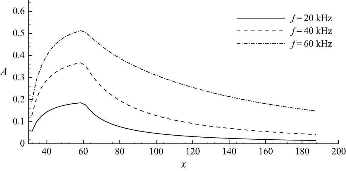
The effect of frequency of the plasma actuators on the streak amplitude is displayed in figure 11. All three frequencies generate similar behaviours, i.e.  $A$ grows with a reduced rate along
 $x$ until the end of the plasma actuation region, and then starts to decrease abruptly. It can be seen that higher frequency results in a larger growth rate, which is a direct result of the increased force amplitude. The streak amplitude at
 $x=60$ increases sublinearly with respect to the frequency, while in figure 3 the magnitude of force has a superlinear relationship with the frequency.
Variation of the streak amplitude  $A$ against frequency with
 $(L_x, L_z)=(30,0.25)$.

4.4. Secondary instabilities of streaks
The asymmetric and symmetric patterns of the total streamwise disturbance with respect to the centreline in the previous section indicate different forms of instabilities. In this section, secondary instabilities of the streaks are investigated in detail by examining two cases specifically, i.e. a narrow layout case  $(L_x,L_z)=(90,0.25)$ and a wide layout case
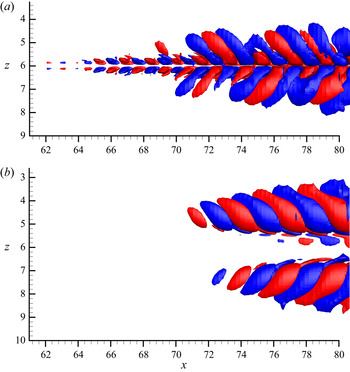
 $(L_x,L_z)=(90,1)$, which have been shown in figure 9(b) and 9(d), respectively. Figure 12 presents the streamwise perturbation
 $u''$ for both the narrow and wide layouts in a zoomed-in view that only covers stage 2. In the narrow layout case, the positive streak in the centre loses stability first, with
 $u''$ appearing in an asymmetric pattern from
 $x=62$. The perturbations then expand to the negative streaks on the side after
 $x=70$, while the asymmetry with respect to
 $z=6$ is maintained. A different observation is seen in the wide layout configuration in figure 12(b):
 $u''$ first starts to appear on the negative streaks at
 $x=72$. Since the instabilities are developed almost simultaneously on their own around the underlying streak, the perturbations are symmetric with respect to
 $z=6$. It seems that
 $L_z$ determines whether the positive streak in the centre loses stability prior to the breakdown of negative streaks, consequently affecting the appearance of
 $u''$, i.e. asymmetric (symmetric) pattern for small (large) values of
 $L_z$. In the rest of this section, we will investigate in detail the secondary instability.
Isosurfaces of streamwise perturbation  $u''=0.005$ (red) and
 $u''=-0.005$ (blue) for (a)
 $(L_x, L_z)=(90,0.25)$ and (b)
 $(L_x, L_z)=(90,1)$.

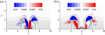
Figure 13 shows the streamwise disturbance  $u''$ as well as the mean flow at
 $x=78$ within stage 2. It can be seen that
 $u''$ is symmetric with respect to
 $z=6$ in the narrow layout and asymmetric in the wide layout, as discussed previously. In both cases, the solid green lines connecting the peak of the mean flow at each contour level bend towards the centre as a result of the interaction between the positive streak at the centre and the lifted negative streaks on the side. In the narrow configuration, the disturbance on the right-hand side shows an asymmetric-like pattern with respect to the inclined negative streak centre, while on the left-hand side the pattern is neither symmetric nor asymmetric. In the wide layout case,
 $u''$ shows a symmetry-like pattern. The disturbances are not completely symmetric or asymmetric with respect to the unstable streak as observed in a model problem where ideal streaks are used (Asai, Minagawa & Nishioka Reference Asai, Minagawa and Nishioka2002; Brandt & Henningson Reference Brandt and Henningson2002). Brandt et al. (Reference Brandt, Schlatter and Henningson2004) used varicose-like/sinuous-like instability to identify the breakdown type in bypass transition subject to free-stream turbulence. We refer to the patterns observed in figure 13 as inclined varicose-like/sinuous-like instability in this work. It is worth noting that here the secondary instability occurs on the negative streaks on each side, while in transition induced by a single roughness element, the instability is observed in the central region around the negative streak. The sinuous instability mode is found in the near wake of a thin roughness element, whereas varicose instability plays a key role in the larger element case (Loiseau et al. Reference Loiseau, Robinet, Cherubini and Leriche2014).
Colour contour of  $u''$ at
 $x=78$ with (a)
 $(L_x, L_z)=(90,0.25)$ and (b)
 $(L_x, L_z)=(90,1)$. Black lines show the contour lines of the streamwise mean velocity
 $\overline {U}$ from
 $0.1$ to
 $1$. Green lines connect the peak of
 $\overline {U}$ at each contour level.

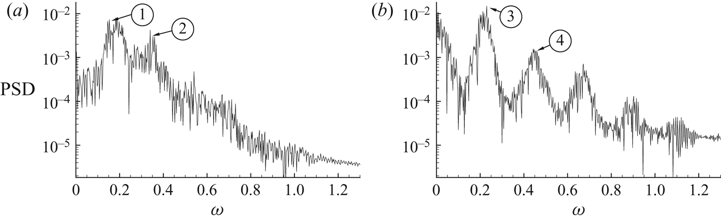
To further investigate the breakdown type, the disturbance velocity is transferred to the Fourier space through discrete Fourier transform. Figure 14 provides the frequency spectra at  $(x,y,z)=(78,2.1,7)$ for the narrow configuration and
 $(x,y,z)=(78,2.1,4.5)$ for the wide configuration, respectively. In figure 14(a) the peak for the narrow configuration is around
 $\omega =0.18$ and broad-banded. The value of the second peak is close to the first one and the remaining peaks at higher frequencies are not clear. In figure 14(b), the peak of the spectrum occurs at
 $\omega =0.22$ and the values for the remaining higher frequencies reduce gradually. A very similar observation is found in the experimental work of Puckert & Rist (Reference Puckert and Rist2018, Reference Puckert and Rist2019), where disturbance developed downstream of a roughness element is investigated. Puckert & Rist (Reference Puckert and Rist2019) also reported a changeover of the Fourier spectra when increasing the Reynolds number. They observed varicose modes at subcritical
 $Re$ where there are distinctive peaks in the Fourier spectra. At supercritical
 $Re$ they found that the varicose and sinuous modes coexist and are coupled by frequency lock-in.


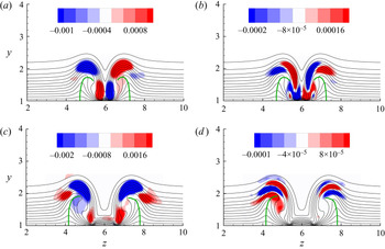
The Fourier mode shape at  $x=78$ at frequencies marked in figure 14 are examined. Figure 15(a,b) presents two representative Fourier mode shapes in the narrow layout case between
 $\omega =0.15$ and
 $\omega =0.35$. In figure 15(a) the Fourier mode exhibits a clear asymmetric shape with respect to the inclined mean flow. On the other hand, in figure 15(b) the mode shape is symmetric, similar to the varicose pattern (Asai et al. Reference Asai, Minagawa and Nishioka2002). It therefore can be concluded that both the sinuous-like and varicose-like types of instability exist in the transition downstream of plasma actuators with narrow spanwise distance. It is worth noting that most of the mode shape that can be identified around the first frequency peak in figure 14(a) is asymmetric while most around the second frequency peak is symmetric, similar to the observation by Puckert & Rist (Reference Puckert and Rist2019). In the case where the sinuous and varicose modes coexist, they also found a sinuous pattern of Fourier modes at a low frequency and a varicose pattern at a high frequency. In the wide layout case shown in figure 15(c,d), Fourier modes are computed at the peak frequencies and the perturbation patterns are similar to that in figure 13(b), confirming the inclined varicose-like instability for the wide configuration.
Contour of streamwise component of Fourier mode for the narrow layout case at (a)  $\omega =0.18$ and (b)
 $\omega =0.29$, which correspond to ① and ② in figure 14(a), and for the wide layout case at (c)
 $\omega =0.225$ and (d)
 $\omega =0.45$, which correspond to ③ and ④ in figure 14(b). Contour lines denote the streamwise mean velocity
 $\overline {U}$ from
 $0.1$ to
 $1$.

4.5. Tilting of disturbance
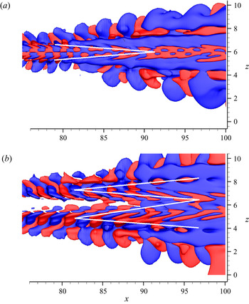
In this section, the third stage in figure 6 starting from  $x=85$ is discussed in detail. Figure 16 shows isosurfaces of the streamwise perturbation
 $u''$ in stage 3 for the narrow and wide layouts, respectively. The velocity perturbation is further tilted along the direction of shear in the region between
 $x=80$ and
 $x=90$ downstream of the instability region where the structures are almost periodic in the streamwise direction. In figure 16(a), the disturbance is inclined towards the centre in the streamwise direction and displays a ‘V’ shape. In figure 16(b), the disturbance near the centre is tilted downstream, while those on the side are tilted upstream, resulting in a ‘W’ shape.
Isosurfaces of  $u''=0.005$ (red) and
 $u''=-0.005$ (blue) for (a)
 $(L_x, L_z)=(90, 0.25)$ and (b)
 $(L_x, L_z)=(90, 1)$. Note here that the positive wall-normal direction points into the paper. Solid white lines are drawn along the disturbance inclination and show a ‘V’ and ‘W’ shape in (a) and (b) , respectively.

To explain the different patterns of inclination, we examine the mean spanwise shear in a  $y\text {--}z$ plane at
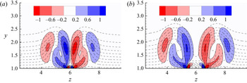
 $x=85$ in figure 17. In both layouts, regions of positive and negative spanwise shear are seen on the flanks of the negative streaks. Since the negative streaks are inclined towards the centre, the mean shear on the side closer to the centre is stronger than that on the other side. In the narrow layout, the streaks are closer and the resulting mean spanwise shear and its gradient in the spanwise direction are stronger than those in the wide layout.
Contour of mean spanwise shear  $\textrm {d}\overline {U}/\textrm {d}z$ at
 $x=85$ for (a)
 $(L_x, L_z)=(90, 0.25)$ and (b)
 $(L_x, L_z)=(90, 1)$. Dashed contour lines denote the streamwise mean velocity
 $\overline {U}$ from 0.1 to 1.

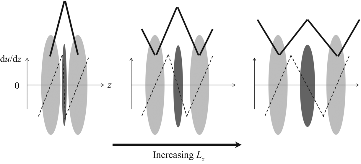
The effect of  $L_z$ on the disturbance is schematically represented in figure 18. The distribution of mean spanwise shear along the spanwise direction is plotted qualitatively by dashed lines. For extremely small values of
 $L_z$, the negative streaks appear close to each other and their width is significantly larger than that of the positive streak. The dashed line in the centre becomes almost vertical, representing a sharp mean spanwise shear gradient at the centre. The spanwise shear in the centre is much stronger, while those on the side become so small that they do not affect the disturbance and can be negligible. The disturbance is tilted forwards by the mean shear in the centre, leading to the ‘V’ shape as seen in figure 16(a). As
 $L_z$ increases, negative streaks become farther away from each other and the positive streak appears wider; consequently, the dashed line in the centre turns anticlockwise. The strength of mean shear in the centre is reduced, while those on the side become strong enough to tilt the disturbance backwards, leaving a ‘W’ shape, with the two sides shorter than those in the middle. As
 $L_z$ further increases, the positive and negative streaks are of similar width to spanwise shear of similar strength. Now the disturbance has a standard ‘W’ shape as shown in figure 16(b).
Schematic plot of streaks induced by plasma actuators. Dark and light grey colours denote positive and negative streaks, respectively. The dashed lines qualitatively represent the distribution of the mean spanwise shear along the spanwise direction. The solid lines indicate the transformation of the ‘V’ shape to the ‘W’ shape as  $L_z$ increases.

5. Linear analysis
The observations in § 4 from DNS results indicate linear dynamics such as secondary instability. These can be studied by linear modal and non-modal analysis, as will be presented in §§ 5.1 and 5.2 below.
5.1. Secondary instability analysis
In this section, linear analysis tools are used to verify and further clarify the DNS observations. In the second stage of the transition process induced by plasma actuation, there is evidence that both the sinuous-like and varicose-like modes exist in the narrow configuration, while in the wide layout, only varicose-like instability is identified. Biglobal stability analysis is used here to illustrate the secondary instability mechanism in stage 2. As the flow develops to turbulence downstream, the time-averaged mean flow  $\overline {\boldsymbol {U}}$ is used as the base flow for all simulations. The algorithms used have been well documented (Schmid & Henningson Reference Schmid and Henningson2001) and will not be elaborated.
The secondary instability is evaluated at a cross-flow plane extracted from various downstream locations in the region from  $x=35$ to
 $x=80$ corresponding to stages
 $1$ and
 $2$ as identified in § 4.2. At each streamwise location, the streamwise wavenumber is varied from
 $\alpha =0$ to
 $\alpha =5$, corresponding to streamwise wavelength of
 $\infty$ and
 $1.25$, respectively. The growth rates of the associated most unstable modes for each pair of
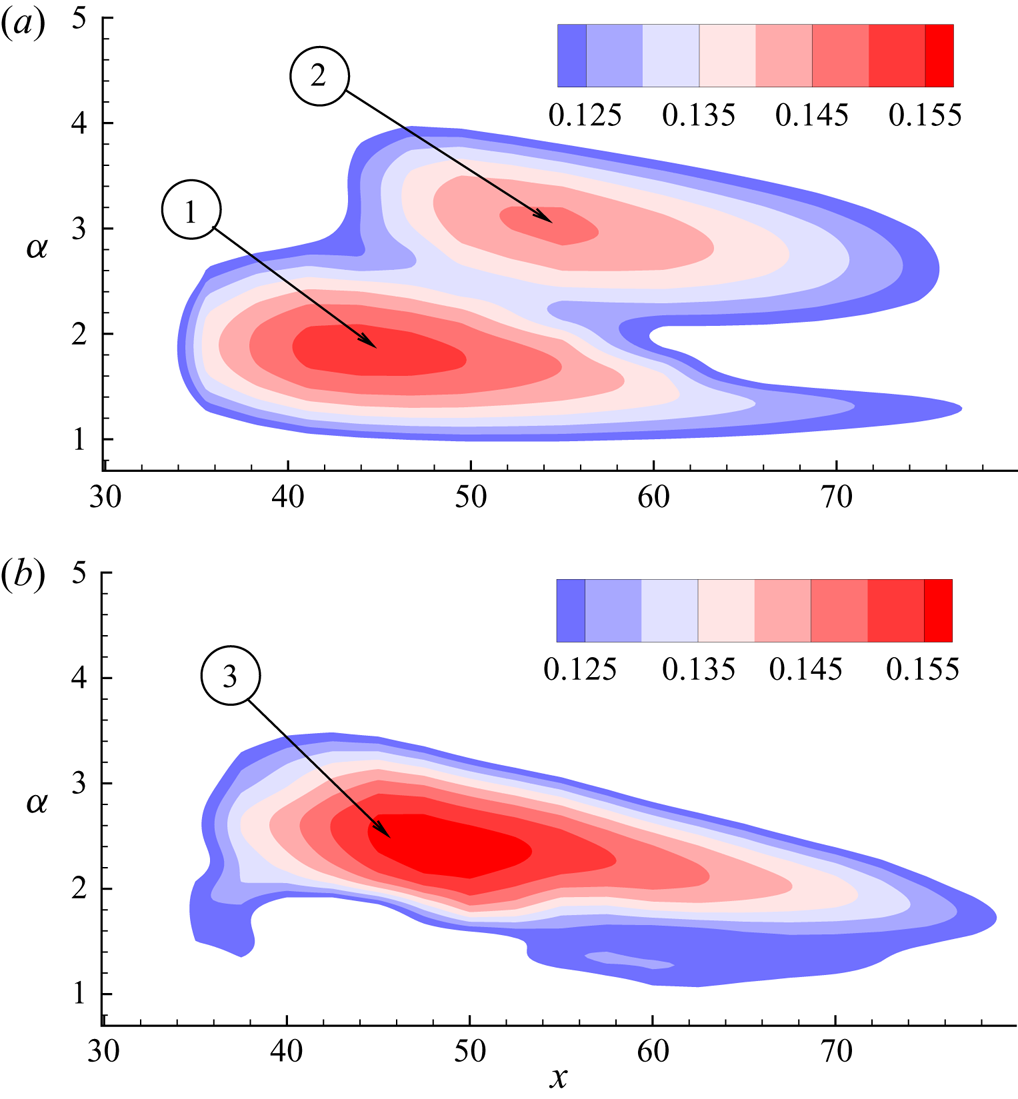
 $(x, \alpha )$ are obtained as plotted in figure 19. For both layouts, the onset of instability of the temporal modes appears at
 $x\approx 35$, at which the streak amplitude
 $A$ reaches around
 $34\,\%$ of the free-stream velocity as shown in figure 10.
The secondary instability growth rate in an  $\alpha \text {--}x$ plane for (a)
 $(L_x, L_z)=(90,0.25)$ and (b)
 $(L_x, L_z)=(90,1)$.

The contour plot of growth rate for the narrow configuration in figure 19(a) has two peaks. The larger peak is located at  $x=45$ and
 $\alpha =1.8$ while the subpeak appears at
 $x=55$ and
 $\alpha =3$. These two peaks correspond to the sinuous and varicose modes and will be illustrated later. Moreover, the temporal frequencies of these two peaks are
 $0.18$ and
 $0.27$, respectively, which are around ① and ② in figure 14(a), corresponding to the sinuous and varicose modes, respectively. In the wide configuration in figure 19(b), the peak of growth rates occurs at
 $x=50$ and
 $\alpha =2.4$. Similar to the narrow layout case, the temporal frequency of the most unstable mode is
 $0.23$, which is in agreement with the peak frequency in figure 14(b). In both cases, the base (mean) flow becomes less unstable at larger
 $x$ even though the streak amplitude continues to increase and reaches a peak at
 $x=80$ in figure 10. This is associated with the change in the base (mean) flow.
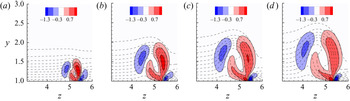
Figure 20 presents the mean spanwise shear of the base flow for the wide layout case as an example at four streamwise positions, which include one upstream of the peak, one at the peak and two downstream of the peak. As  $x$ increases, the base streak grows in size. However, the change in the mean flow shape is different and leads to non-monotonic variation of the mean spanwise shear. In order to compare the mean shear clearly, three positive and negative levels are shown in figure 20. From
 $x=35$ to
 $x=50$, the relative distribution of contour levels is almost the same and only the size of the region is expanding. The increase of mean shear leads to the increase of the growth rate from
 $x=35$ to
 $x=50$ in figure 19(b). From
 $x=50$ onwards, although the overall region continues to expand as a result of the streak growth, the region of the highest contour level becomes smaller and even disappears at
 $x=70$. Therefore, the strength of the mean spanwise shear is the largest at
 $x=50$, at which the mean flow shows the largest growth rate of secondary instability. Similar observations are made in the narrow layout case, i.e.
 $\textrm {d}\overline {U}/\textrm {d}z$ at the peak location
 $x=45$ is the strongest, and is therefore not presented.
Contour of mean spanwise shear  $\textrm {d}\overline {U}/\textrm {d}z$ for
 $(L_x, L_z)=(90,1)$ at (a)
 $x=35$, (b)
 $x=50$, (c)
 $x=60$ and (d)
 $x=70$. Dashed contour lines denote the streamwise mean velocity
 $\overline {U}$ from 0.1 to 1. Only half of the domain in the spanwise direction is presented.

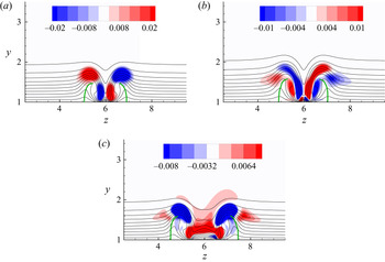
Representative eigenmodes of the secondary instability near the peaks in the narrow and wide layouts are illustrated in figure 21, along with line contours of the streaky mean profile  $\overline {\boldsymbol {U}}$. For the narrow layout, the mode shape at the lower peak is asymmetric with respect to the negative streak, and that at the higher peak is symmetric; while for the wide layout, the secondary instability is symmetric. These confirm that both types of instability exist in the narrow layout case, while in the wide layout case there are only varicose-like modes.
Secondary instability modes at: (a)  $x=45$,
 $\alpha =1.8$, corresponding to ① in figure 19(a); (b)
 $x=55$,
 $\alpha =3$, corresponding to ② in figure 19(b); and (c)
 $x=45$,
 $\alpha =2.3$ , corresponding to ③ in figure 19(b). Solid contour lines denote the streamwise mean velocity
 $\overline {U}$ from 0.1 to 1.

5.2. Transient growth analysis
As mentioned previously, plasma actuators are analogous to roughness elements. It has been found that transient growth plays a significant role in roughness-induced transition (White Reference White2002; White, Rice & Ergin Reference White, Rice and Ergin2005; Downs et al. Reference Downs, White and Denissen2008). In this section, linear optimal transient growth analysis is performed to further investigate stage 3 from the DNS results in § 4.5. Similar to before, time-averaged mean flow  $\overline {\boldsymbol {U}}$ is adopted as the base flow. Initial conditions that result in the largest transient energy growth
 $G$ over a time horizon
 $T$ is obtained, with
 \begin{equation} G=\frac{E(T)}{E(0)}, \end{equation}
where  $E$ denotes the kinetic energy of the perturbation integrated over the computational domain
 $\varOmega$. The numerical solver used for the transient growth analysis involves solving the linearised NS equation and its adjoint, and has been verified in previous works (Barkley et al. Reference Barkley, Blackburn and Sherwin2008; Mao & Hussain Reference Mao and Hussain2017).
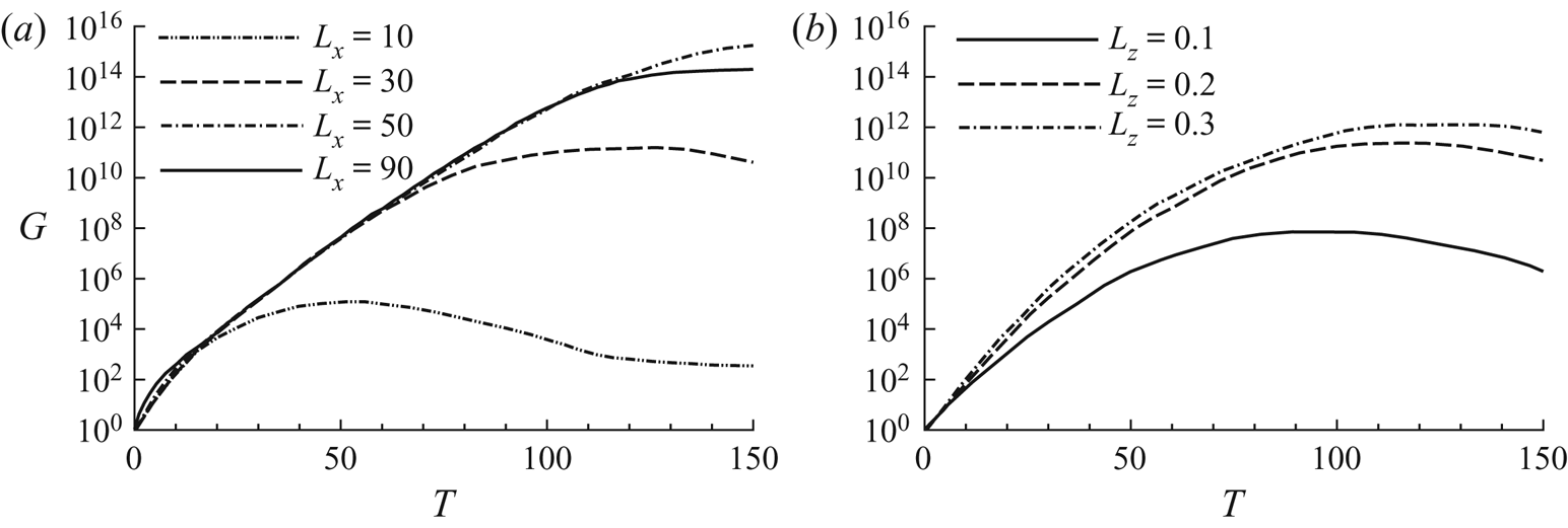
The variation of the maximum growth  $G$ with respect to
 $T$ at different
 $L_x$ and
 $L_z$ is presented in figure 22. In figure 22(a), before reaching the peak,
 $G$ increases with
 $T$ at a similar rate for all cases. Moreover, larger
 $L_x$ results in a higher peak value of
 $G$ because longer actuators lead to larger streak amplitude, as shown in figure 8, in agreement with the findings in Cherubini et al. (Reference Cherubini, De Tullio, De Palma and Pascazio2013), where transient growth analysis of flow past a roughness element was performed. The effect of
 $L_z$ on
 $G$ is similar, as seen in figure 22(b). The value of
 $G$ for
 $(L_x,L_z)=(90,0.1)$, which leads to only streaks without breakdown, is significantly smaller than those with larger
 $L_z$ that result in turbulence.
Maximum transient energy growth  $G$ versus
 $T$ for (a)
 $L_z=0.25$ and various values of
 $L_x$, and (b)
 $L_x=90$ and various values of
 $L_z$.

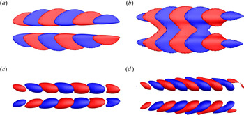
The streamwise component of the initial condition that leads to the largest transient energy growth for the narrow and wide layout cases is presented in figures 23(a) and 23(b), respectively. In figure 23(a), the initial streamwise velocity resembles the optimal response for neither the varicose nor the sinuous perturbations found in the literature, as we have seen that both types of instability modes exist. In figure 23(b), the streamwise component on each side, concentrated in the region of strong wall-normal shear on the top of the streak, resembles the optimal initial streamwise velocity obtained for the varicose perturbation in Hœpffner, Brandt & Henningson (Reference Hœpffner, Brandt and Henningson2005). This is another proof of the varicose-like instabilities on the negative streaks in the wide layout. The velocity component in the narrow layout has a similar pattern as that in the wide layout, but is slightly tilted in the streamwise direction. Moreover, the streamwise velocity is asymmetric with respect to the centre in the narrow configuration and symmetric in the wide configuration, which is in agreement with the observations from DNS.
Isosurfaces of streamwise velocity of the initial conditions yielding the maximum energy growth (a,b) and their optimal response at  $t=90$ (c,d). Panels (a,c) present the narrow layout case with
 $(L_x, L_z)=(90,0.25)$ while panels (b,d) present the wide layout case with
 $(L_x, L_z)=(90,1)$. The plots show the
 $x\text {--}z$ plane view. The isosurfaces represent areas where the value equals
 $0.2$ of the maxima/minima.

The optimal responses at  $t=90$ for the initial conditions in figure 23(a,b) are illustrated in figure 23(c,d). In both layouts, the streamwise velocity component is the most amplified, which is also reported in previous work (Hœpffner et al. Reference Hœpffner, Brandt and Henningson2005; Cherubini et al. Reference Cherubini, De Tullio, De Palma and Pascazio2013).
Figure 24 presents the same flow as in figure 23, but in the  $x\text {--}y$ plane. In both cases, the streamwise components are initially backward-leaning against the shear. In figure 24(c,d), the structures are tilted to be forward-leaning by the shear, suggesting the Orr mechanism in which perturbations gain transient energy growth when they are tilted from backward-leaning to normal and then decay when tilted to be forward-leaning. However, inspecting the history of flow development (not shown here), we observe that the forward-leaning structures only appear at
 $t<10$. In figure 22, the growth lasts to
 $t \sim 100$, indicating that the Orr mechanism only contributes to the energy growth initially and the lift-up effect has a significant role in the energy growth at later time. Similar observations were reported by Hack & Moin (Reference Hack and Moin2017), who found that in non-parallel flow the energy growth of the most highly amplified perturbations is attributed to the combined action of the lift-up and Orr mechanism.
Isosurfaces of streamwise velocity of the initial conditions yielding the maximum energy growth (a,b) and their optimal response at  $t=90$ (c,d). Panels (a,c) present the narrow layout case with
 $(L_x, L_z)=(90,0.25)$ while panels (b,d) present the wide layout case with
 $(L_x, L_z)=(90,1)$. The plots show the
 $x\text {--}y$ plane view. The isosurfaces represent areas where the value equals
 $0.2$ of the maxima/minima.

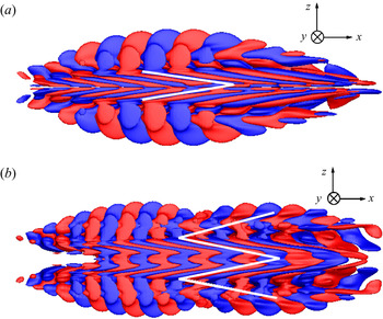
The isosurfaces in figures 23 and 24 represent values equal to  $0.2$ of the maxima/minima and the flow structures are inclined in the streamwise direction due to the mean spanwise shear caused by the positive streak at the centre. In order to link the transient growth mode with previous DNS results, figure 25 displays the optimal response of streamwise velocity, similar to that in figure 23(c,d) but with the isosurfaces representing a much smaller value that corresponds to 0.022 of the maxima/minima. The plots are presented with positive wall-normal direction pointing into the paper. The ‘V’ shape in the narrow layout and ‘W’ shape in the wide layout observed in figure 16 can be clearly seen here, which support the findings in the DNS. Another observation that supports previous ones is that in figure 25(a) the velocity component starts to appear around the centre before expanding in the spanwise direction, while in the wide layout case in figure 25(b), the perturbations first appear on each side simultaneously and expand on their own, before merging together and then the Orr mechanism becomes dominant.
Isosurfaces of streamwise velocity of the final conditions yielding the maximum energy growth at  $T=120$ for (a)
 $(L_x, L_z)=(90,0.25)$ and (b)
 $(L_x, L_z)=(90,1)$. Both panels show the
 $x$–
 $z$ plane with positive wall-normal direction pointing into the paper. The isosurfaces represent areas where the value equals
 $0.022$ of the maxima/minima.

6. Conclusion
The response of a boundary layer flow over a flat plate to the actuation of a pair of DBD plasma actuators mounted on the plate is investigated numerically. A four-species plasma–fluid model is used to model the EHD body force generated by the plasma actuators. A two-dimensional steady plasma force distribution is computed from a plasma solver and used to drive the transition in the three-dimensional boundary layer.
The body force generated by the plasma actuators results in a pair of counter-rotating streamwise vortices that lead to the formation of a high-speed streak in the centre and two low-speed streaks on either side. Both the streamwise length of actuators  $(L_x)$ and the spanwise distance between the actuators
 $(L_z)$ affect the flow development significantly. For small values of
 $L_x$, the streaks initially grow and start to decay immediately beyond the actuator region. Larger
 $L_x$ results in larger streak amplitude and bypass transition through a turbulent wedge. On the other hand,
 $L_z$ determines the peak value of streak amplitude. For
 $L_z$ below a certain value, the peak streak amplitude does not exceed the critical value and is maintained over the plasma region. In cases with larger
 $L_z$, bypass transition occurs at a similar location.
The bypass transition downstream of the plasma actuators can be divided into four stages: generation of streaks, secondary instability, tilting of perturbations and turbulent wedge. The second and third stages are investigated in detail through two cases: a narrow layout and a wide layout. In the former case, the positive and negative streaks are close in the spanwise direction, resulting in strong mean spanwise shear. This leads to secondary instability with an asymmetric pattern first appearing on the high-speed streak in the centre. The low-speed streaks lose stability afterwards, with evidence of both inclined sinuous-like and varicose-like modes. The perturbations remain asymmetric with respect to the centre. In the following tilting stage, the mean shear at the centre dominates and the perturbations appear in a ‘V’ pattern. In the latter case, the low-speed streak on each side experiences inclined varicose-like secondary instability simultaneously, and therefore the perturbations have a symmetric pattern with respect to the centre. In the third stage, the perturbations expand in the spanwise direction via shear, which results in a ‘W’ pattern.
Biglobal stability analysis is performed using the mean flow from DNS as the base profile to further examine the secondary instabilities. In the narrow configuration, two peaks of the growth rate on the streamwise location versus streamwise wavenumber plane are observed, corresponding to an inclined sinuous-like instability and a varicose-like one, while in the wide layout the mode shape at the peak of the growth rate is inclined varicose-like. The optimal initial condition from transient growth analysis is symmetric with respect to the centre for the wide configuration and asymmetric for the narrow configuration. The ‘V’ and ‘W’ patterns due to the shear are also observed in the flow response for the narrow and wide layout, respectively. In summary, the findings from DNS are confirmed by these linear analyses, which further reveal the mechanism of the perturbation development.
Funding
This work was supported by the Marie Skłodowska-Curie Research and Innovation Staff Exchanges programme (Grant No. 777717).
Declaration of interests
The authors report no conflict of interest.