2 LEAST SQUARES MODEL AVERAGING

Suppose we have n independent observations $\{(y_i, \mathbf {x}_i)\colon i=1,\ldots ,n\}$ , where $y_i$ is a scalar response and $\mathbf {x}_i=(x_{i1},x_{i2},\ldots )$ is a vector of countably infinite covariates. Consider the linear regression model

(2.1) $$ \begin{align} y_i=\mu_i+e_i=\sum_{j=1}^{\infty} \beta_jx_{ij}+e_i, \end{align} $$

where $e_1,\ldots , e_n$ are independent and identically distributed (i.i.d.) errors satisfying $E(e_i\mid \mathbf {x}_i)=0$ and $E(e_i^2\mid \mathbf {x}_i)=\sigma ^2$ , and $\beta _j$ ’s are unknown parameters. In matrix notation, (2.1) can be written as $\mathbf {y}=\boldsymbol {\mu }+\mathbf {e}$ , where $\mathbf {y}=(y_1,\ldots ,y_n)^{\top }$ , $\boldsymbol {\mu }=(\mu _1,\ldots ,\mu _n)^{\top }$ , and $\mathbf {e}=(e_1,\ldots ,e_n)^{\top }$ .

To estimate the true mean vector $\boldsymbol {\mu }$ , we consider $M_n$ nested candidate models for model averaging, where the mth model uses the first $k_m$ covariates and $0<k_1<\cdots <k_{M_n}<\infty $ . Both $k_{M_n}$ and $M_n$ can be diverging to infinity as $n\to \infty $ . Let $\mathbf {X}_m$ be the $n \times k_m$ design matrix of the mth model. We assume that $\mathbf {X}_m$ is of full column rank for every $m \in \{1,\ldots ,M_n\}$ . Then, under the mth model, the estimator of $\boldsymbol {\mu }$ is $\widehat {\boldsymbol {\mu }}_m=\mathbf {P}_m \mathbf {y}$ , where $\mathbf {P}_m=\mathbf {X}_m(\mathbf {X}_m^{\top }\mathbf {X}_m)^{-1}\mathbf {X}_m^{\top }$ . Let $\mathbf {w}=(w_1,\ldots ,w_{M_n})^{\top }$ be a weight vector belonging to the unit simplex in $\mathbb {R}^{M_n}$ :

$$ \begin{align*} \mathcal{H}_n=\left\{\mathbf{w}\in [0, 1]^{M_n}\colon \sum_{m=1}^{M_n} w_m=1\right\}\!. \end{align*} $$

Then, the model averaging estimator of $\boldsymbol {\mu }$ with weights $\mathbf {w}$ is $\widehat {\boldsymbol {\mu }}(\mathbf {w})=\sum _{m=1}^{M_n} w_m \widehat {\boldsymbol {\mu }}_m=\mathbf {P}(\mathbf {w})\mathbf {y}$ , where $\mathbf {P}(\mathbf {w})=\sum _{m=1}^{M_n} w_m\mathbf {P}_m$ . Let $\mathbf {I}_n$ be the identity matrix of size n, and let $\|\cdot \|$ be the Euclidean norm. Following Zhang et al. (Reference Zhang, Zou, Liang and Carroll2020), the weight vector $\mathbf {w}$ is selected by minimizing the criterion

(2.2) $$ \begin{align} \mathcal{G}_n(\mathbf{w})=\|\{\mathbf{I}_n-\mathbf{P}(\mathbf{w})\}\mathbf{y}\|^2+\phi_n\widehat{\sigma}^2 \mathbf{w}^{\top}\mathbf{K}, \end{align} $$

where $\widehat {\sigma }^2=(n-k_{M_n})^{-1}\mathbf {y}^{\top }(\mathbf {I}_n-\mathbf {P}_{M_n})\mathbf {y}$ is an estimator of $\sigma ^2$ , $\mathbf {K}=(k_1,\ldots ,k_{M_n})^{\top }$ , and $\phi _n$ is a penalty factor that may depend on n. Two common choices for $\phi _n$ are $2$ and $\log n$ . When $\phi _n=2$ , (2.2) is the Mallows criterion of Hansen (Reference Hansen2007). When all elements of $\mathbf {w}$ are 0 or 1, the weight selection criterion (2.2) corresponds to AIC for $\phi _n=2$ and to BIC for $\phi _n=\log n$ . Note that Fang, Yang, and Tian (Reference Fang, Yang and Tian2022) proposed a cross-validation procedure for selecting $\phi _n$ between $2$ and $\log n$ . Finally, the selected weight vector is defined as $\widehat {\mathbf {w}}=(\widehat {w}_1,\ldots ,\widehat {w}_{M_n})^{\top }=\mathrm {argmin}_{\mathbf {w}\in {\mathcal {H}_{n}}} \mathcal {G}_{n}(\mathbf {w})$ .

Define the squared error loss as $L_n(\mathbf {w})=\|\boldsymbol {\mu }-\widehat {\boldsymbol {\mu }}(\mathbf {w})\|^2$ and the corresponding risk (the expected squared error) as $R_n(\mathbf {w})=E\{L_n(\mathbf {w})\mid \mathbf {x}_1,\ldots ,\mathbf {x}_n\}$ . Both are useful measures of the accuracy of $\widehat {\boldsymbol {\mu }}(\mathbf {w})$ for $\boldsymbol {\mu }$ . In the model averaging literature, two types of asymptotic optimality are commonly considered: asymptotic loss optimality and asymptotic risk optimality. Specifically, we say that $\widehat {\mathbf {w}}$ is asymptotically loss optimal if

(OPT.1) $$ \begin{align} L_n(\widehat{\mathbf{w}})/\inf_{\mathbf{w}\in \mathcal{H}_n} L_n(\mathbf{w})\to_p 1, \end{align} $$

and asymptotically risk optimal if

(OPT.2) $$ \begin{align} R_n(\widehat{\mathbf{w}})/\inf_{\mathbf{w}\in \mathcal{H}_n} R_n(\mathbf{w})\to_p 1. \end{align} $$

Here, $\to _p$ denotes convergence in probability. All limiting processes in this article are with respect to $n\to \infty $ . Note that (OPT.1) means that the squared error loss of the model averaging estimator is asymptotically as small as that of the infeasible best possible averaging estimator, and (OPT.2) is a similar statement about the expected squared error. In the existing literature (Wan et al., Reference Wan, Zhang and Zou2010; Zhang et al., Reference Zhang, Zou, Liang and Carroll2020; Zhang, Reference Zhang2021; Peng et al., Reference Peng, Li and Yang2025), these two types of asymptotic optimality are typically considered as equivalent; see below for further discussion.

When $\phi _n=2$ (MMA), Hansen (Reference Hansen2007) established the asymptotic loss optimality of $\widehat {\mathbf {w}}$ . However, this result requires weights to be confined to the discrete set

$$ \begin{align*} \mathcal{H}_n(N)=\left\{\mathbf{w}\colon w_m\in \left\{0,\frac{1}{N},\frac{2}{N},\ldots,1\right\},\sum_{m=1}^{M_n} w_m=1\right\}\!, \end{align*} $$

where N is a fixed positive integer. Note that model averaging restricted to $\mathcal {H}_n(1)$ reduces to model selection. Subsequently, Wan et al. (Reference Wan, Zhang and Zou2010), Zhang (Reference Zhang2021), and Peng et al. (Reference Peng, Li and Yang2025) demonstrated that $\widehat {\mathbf {w}}$ is asymptotically loss optimal over the continuous weight set $\mathcal {H}_n$ . Their proofs in fact imply the asymptotic risk optimality of $\widehat {\mathbf {w}}$ as well. When $\phi _n\to \infty $ (PMA), Zhang et al. (Reference Zhang, Zou, Liang and Carroll2020) justified both the asymptotic loss and risk optimality of $\widehat {\mathbf {w}}$ . A key prerequisite for these results is that $\xi _n=\inf _{\mathbf {w}\in \mathcal {H}_n} R_n(\mathbf {w})\to \infty $ . This condition implies that there are no candidate models with fixed dimensions for which the approximation error is zero (see also Hansen, Reference Hansen2007). Consequently, the aforementioned results do not apply to the case where a true candidate model with fixed dimension exists. Moreover, in this case, it remains unclear whether the two types of asymptotic optimality hold simultaneously.

Our aim is to investigate both the asymptotic loss and risk optimality of $\widehat {\mathbf {w}}$ when the true model is included among the candidate models. Let $\mathcal {A}_m=\{1,\ldots ,k_m\}$ , and let $\mathcal {A}_m^c$ denote its complement. We assume that there exists an integer $M_0$ such that $(\beta _j, j\in \mathcal {A}_{M_0+1}\cap \mathcal {A}_{M_0}^c)^{\top }\neq \mathbf {0}$ and $\beta _j=0$ for all $j>k_{M_0+1}$ . Consequently, the first $M_0$ candidate models are under-fitted, the $(M_0+1)$ th model is defined as the “true model,” and the remaining models are over-fitted. We further assume that $M_0\geq 1$ and $M_n>M_0+1$ , so that the candidate model set contains at least one under-fitted model and one over-fitted model. Note that $k_{M_0+1}$ is the dimension of the true model, and both $k_{M_0+1}$ and $M_0$ are allowed to diverge.

3 EXISTING RESULTS AND DISCUSSION

In a recent study, Fang et al. (Reference Fang, Yuan and Tian2023) established conditions that determine whether $\widehat {\mathbf {w}}$ achieves the asymptotic loss optimality (OPT.1) when the true model is included among the candidate models (see their Lemma 1 and Theorem 5 for details). However, due to technical difficulty, their results rely on the following slightly special weight set:

$$ \begin{align*} \mathcal{H}_n^{\delta}=\left\{\mathbf{w}\in \mathcal{H}_n\colon \sum_{m<M_0+1} w_m=0~\text{or}~\sum_{m<M_0+1} w_m\geq \delta n^{-\tau_0}\right\}\!. \end{align*} $$

Here, $\delta $ is a positive constant which can be arbitrarily small, and $\tau _0$ is a positive constant satisfying $\sum _{j\in \mathcal {A}_{M_0+1}\cap \mathcal {A}_{M_0}^c} \beta _j^2\geq c_{\tau _0} n^{-\tau _0}$ for some positive constant $c_{\tau _0}$ . Compared to $\mathcal {H}_n$ , the special weight set $\mathcal {H}_n^{\delta }$ excludes the case of $0<\sum _{m<M_0+1} w_m<\delta n^{-\tau _0}$ . As a result, the weights assigned to the under-fitted models must either be zero or have a total sum at least $\delta n^{-\tau _0}$ . Note that when $\delta $ is sufficiently small or n is large, $\mathcal {H}_n^{\delta }$ includes the discrete weight set $\mathcal {H}_n(N)$ considered by Hansen (Reference Hansen2007) and Hansen and Racine (Reference Hansen and Racine2012).

By an abuse of notation, we still use $\widehat {\mathbf {w}}$ in this section to denote $\mathrm {argmin}_{\mathbf {w}\in \mathcal {H}_n^{\delta }} \mathcal {G}_n(\mathbf {w})$ . We summarize the results in Theorem 5 of Fang et al. (Reference Fang, Yuan and Tian2023) as follows:

1. (i) When $\phi _n=\log n$ , as long as the true model dimension does not diverge too fast, $\widehat {\mathbf {w}}$ is asymptotically loss optimal in the sense that $L_n(\widehat {\mathbf {w}})/\inf _{\mathbf {w}\in \mathcal {H}_n^{\delta }} L_n(\mathbf {w})\to _p 1$ by pushing all the weights to the true model.

2. (ii) When $\phi _n=2$ and the model dimensions are fixed, asymptotic loss optimality does not hold in the sense that $L_n(\widehat {\mathbf {w}})/\inf _{\mathbf {w}\in \mathcal {H}_n^{\delta }} L_n(\mathbf {w})\nrightarrow _p 1$ since the model averaging method puts weights on the over-fitted models with a positive probability.

In the area of model selection, it is well known that in a parametric framework, AIC is not asymptotically loss optimal, whereas BIC is due to its consistency (Shao, Reference Shao1997). Consequently, Results (i) and (ii) are similar to the corresponding asymptotic behaviors of BIC and AIC, respectively.

Denote by $\mathbf {w}_m^0$ an $M_n\times 1$ vector in which the mth element is one and the others are zeros. Let $\mathbf {w}^*=(w_1^*,\ldots , w_{M_n}^*)^{\top }=\mathrm {argmin}_{\mathbf {w}\in \mathcal {H}_n^{\delta }} L_n(\mathbf {w})$ . The proof of the above results of Fang et al. (Reference Fang, Yuan and Tian2023) is divided into the following two steps.

1. Step 1. Prove that $\Pr (\mathbf {w}^*=\mathbf {w}_{M_0+1}^0)\to 1$ .

2. Step 2. Analyze whether $L_n(\widehat {\mathbf {w}})/L_n(\mathbf {w}_{M_0+1}^0)$ converges to 1 in probability.

Steps 1 and 2 correspond to the results in their Lemma 1 and Theorem 5, respectively. The special weight set $\mathcal {H}_n^{\delta }$ is mainly utilized in Step 1, where it enforces either $\sum _{m<M_0+1} w_m^*=0$ or $\sum _{m<M_0+1} w_m^*\geq \delta n^{-\tau _0}$ . Lemma 1 of Fang et al. (Reference Fang, Yuan and Tian2023) showed that $\Pr (\sum _{m<M_0+1} w_m^*\geq \delta n^{-\tau _0})\to 0$ and $\sum _{m>M_0+1} w_m^*=0$ . Therefore, $\Pr (\mathbf {w}^*=\mathbf {w}_{M_0+1}^0)\to 1$ , which implies $\Pr \{\inf _{\mathbf {w}\in \mathcal {H}_n^{\delta }} L_n(\mathbf {w})=L_n(\mathbf {w}_{M_0+1}^0)\}\to 1$ . Consequently, $L_n(\widehat {\mathbf {w}})/\inf _{\mathbf {w}\in \mathcal {H}_n^{\delta }} L_n(\mathbf {w})$ and $L_n(\widehat {\mathbf {w}})/L_n(\mathbf {w}_{M_0+1}^0)$ share the same asymptotic behavior. After finishing Step 1, the remaining work is Step 2, which relies on the asymptotic properties of the estimated weights for the under-fitted and over-fitted models. These properties have been extensively studied in the literature, such as Zhang and Liu (Reference Zhang and Liu2019) and Zhang et al. (Reference Zhang, Zou, Liang and Carroll2020).

In practice, the special weight set $\mathcal {H}_n^{\delta }$ is not useful because we do not know which models are under-fitted, and the set depends on unknown constants $\delta $ and $\tau _0$ . On the other hand, as shown in Theorem 6 of Xu and Zhang (Reference Xu and Zhang2025), restricting model averaging to the discrete weight set $\mathcal {H}_n(N)$ may enlarge the optimal risk. Therefore, it is necessary to adopt the usual weight set $\mathcal {H}_n$ for model averaging. A natural question is whether Lemma 1 and Theorem 5 of Fang et al. (Reference Fang, Yuan and Tian2023) remain valid when $\mathcal {H}_n^{\delta }$ is replaced by $\mathcal {H}_n$ . Let $\mathbf {w}^L=\mathrm {argmin}_{\mathbf {w}\in \mathcal {H}_n} L_n(\mathbf {w})$ . In Section S.1.1 of the Supplementary Material, we provide a toy example to illustrate that $\Pr (\mathbf {w}^L=\mathbf {w}_{M_0+1}^0)\nrightarrow 1$ and that the asymptotic loss optimality (OPT.1) does not hold when $\phi _n=\log n$ , which is opposite to Result (i), that is, Theorem 5(1) of Fang et al. (Reference Fang, Yuan and Tian2023). In the next section, we show that these findings remain valid when the true model dimension is fixed, and we also investigate the asymptotic risk optimality (OPT.2), a topic that has not been studied by Fang et al. (Reference Fang, Yuan and Tian2023).

4 MAIN RESULTS

In this section, we investigate both the asymptotic loss and risk optimality of $\widehat {\mathbf {w}}$ . As pointed out in Section 3, the result $\Pr (\mathbf {w}^L=\mathbf {w}_{M_0+1}^0)\to 1$ may not hold (see also Section S.3.1 of the Supplementary Material). This suggests that the proof procedures used by Fang et al. (Reference Fang, Yuan and Tian2023), that is, Steps 1 and 2 in Section 3, may not be applicable. Observe that

$$ \begin{align*} \frac{L_n(\widehat{\mathbf{w}})}{\inf_{\mathbf{w}\in \mathcal{H}_n} L_n(\mathbf{w})}=\frac{L_n(\widehat{\mathbf{w}})}{L_n(\mathbf{w}_{M_0+1}^0)}\times \frac{L_n(\mathbf{w}_{M_0+1}^0)}{\inf_{\mathbf{w}\in \mathcal{H}_n} L_n(\mathbf{w})}. \end{align*} $$

Therefore, if $L_n(\widehat {\mathbf {w}})/L_n(\mathbf {w}_{M_0+1}^0)\to _p 1$ , then the asymptotic loss optimality (OPT.1) holds if and only if $L_n(\mathbf {w}_{M_0+1}^0)/\inf _{\mathbf {w}\in \mathcal {H}_n} L_n(\mathbf {w})\to _p 1$ . Similarly, if $R_n(\widehat {\mathbf {w}})/R_n(\mathbf {w}_{M_0+1}^0)\to _p 1$ , then the asymptotic risk optimality (OPT.2) holds if and only if $R_n(\mathbf {w}_{M_0+1}^0)/\inf _{\mathbf {w}\in \mathcal {H}_n} R_n(\mathbf {w})\to _p 1$ . In Section S.2 of the Supplementary Material, we show that $L_n(\widehat {\mathbf {w}})/L_n(\mathbf {w}_{M_0+1}^0)\to _p 1$ and $R_n(\widehat {\mathbf {w}})/R_n(\mathbf {w}_{M_0+1}^0)\to _p 1$ when $\phi _n=\log n$ under certain conditions. Consequently, it remains to investigate whether the true model is asymptotically loss or risk optimal.

Throughout this article, we assume that $E(|e_i|^{4+\zeta }\mid \mathbf {x}_i)<\infty $ almost surely for some $\zeta>0$ . Let $\lambda _{\min }(\mathbf {M})$ be the minimum eigenvalue of a positive-definite matrix $\mathbf {M}$ . We first state the regularity conditions required for main results.

Conditions (C1)–(C4) are commonly adopted in the model averaging literature (Zhang et al., Reference Zhang, Zou, Liang and Carroll2020; Fang et al., Reference Fang, Yuan and Tian2023). See Section S.1.2 of the Supplementary Material for a detailed discussion. Let $\eta _n=\sum _{j\in \mathcal {A}_{M_0+1}\cap \mathcal {A}_{M_0}^c} \beta _j^2$ . Note that $\eta _n$ measures the difference between the true model and the largest under-fitted model.

4.1 Asymptotic Loss Optimality

In this section, we aim to determine the conditions under which $\widehat {\mathbf {w}}$ achieves the asymptotic loss optimality (OPT.1), and the conditions under which it does not in the sense that $L_n(\widehat {\mathbf {w}})/\inf _{\mathbf {w}\in \mathcal {H}_n} L_n(\mathbf {w})\nrightarrow _p 1$ . As mentioned at the beginning of this section, we first explore whether the true model is asymptotically loss optimal or not.

Lemma 1. Assume that Conditions (C1) and (C2) are satisfied.

1. (i) If $k_{M_0+1}$ is fixed and Condition (C4) is satisfied, then

   $$ \begin{align*} L_n(\mathbf{w}_{M_0+1}^0)/\inf_{\mathbf{w}\in \mathcal{H}_n} L_n(\mathbf{w}) \nrightarrow_p 1. \end{align*} $$

2. (ii) If $k_{M_0+1}\to \infty $ , $(k_{M_0+1}-k_1)/(n\eta _n)\to 0$ , and $M_0/(k_{M_0+1}\eta _n)\to 0$ , then

   $$ \begin{align*} L_n(\mathbf{w}_{M_0+1}^0)/\inf_{\mathbf{w}\in \mathcal{H}_n} L_n(\mathbf{w}) \to_p 1. \end{align*} $$

Lemma 1(i) shows that when the true model dimension is fixed, the true model is not asymptotically loss optimal. This is due to the presence of under-fitted models and their impact on the optimal loss cannot be asymptotically eliminated. This result also confirms that $\Pr (\mathbf {w}^L=\mathbf {w}_{M_0+1}^0)\nrightarrow 1$ when the true model dimension is fixed. Further discussion of Lemma 1(i) is provided in Sections S.1.3 and S.3.2 of the Supplementary Material.

Lemma 1(ii) shows that when the true model dimension diverges, but not too fast, and the condition $M_0/(k_{M_0+1}\eta _n)\to 0$ holds, the true model is asymptotically loss optimal. The key condition $M_0/(k_{M_0+1}\eta _n)\to 0$ requires that $k_{M_0+1}$ diverges at a faster rate than $M_0/\eta _n$ , which ensures that the impact of the under-fitted models on the optimal loss can be asymptotically eliminated. Specifically, in the proof of this lemma, we show that

$$ \begin{align*} \inf_{\mathbf{w}\in \mathcal{H}_n} L_n(\mathbf{w})=L_n(\mathbf{w}_{M_0+1}^0)-\{O_p(M_0/\eta_n)+o_p(k_{M_0+1})\}, \end{align*} $$

where the second term on the right-hand side is attributable to the under-fitted models. Since $L_n(\mathbf {w}_{M_0+1}^0)/(\sigma ^2 k_{M_0+1})\to _p 1$ , the condition $M_0/(k_{M_0+1}\eta _n)\to 0$ ensures that this term is of order $o_p\{L_n(\mathbf {w}_{M_0+1}^0)\}$ . Consequently, the impact of the under-fitted models on the optimal loss is asymptotically negligible compared to the loss of the true model. This explains why the result in Lemma 1(ii) holds. Further discussion of the condition $M_0/(k_{M_0+1}\eta _n)\to 0$ is provided in Section S.3.3 of the Supplementary Material. If the error $e_i$ conditional on $\mathbf {x}_i$ is sub-Gaussian, then this condition can be relaxed to $\log M_0/(k_{M_0+1}\eta _n)\to 0$ (see Section S.1.3 of the Supplementary Material for details).

Remark 1. In Section S.1.4 of the Supplementary Material, we further investigate the asymptotic loss optimality of the true model when the weights are restricted to the special weight set $\mathcal {H}_n(N)$ or $\mathcal {H}_n^{\delta }$ . In particular, if $k_{M_0+1}$ is fixed and $\tau _0\in (0, 1/4)$ for $\mathcal {H}_n^{\delta }$ , then

$$ \begin{align*} L_n(\mathbf{w}_{M_0+1}^0)/\inf_{\mathbf{w}\in \mathcal{H}_n(N)} L_n(\mathbf{w}) \to_p 1\quad \text{and}\quad L_n(\mathbf{w}_{M_0+1}^0)/\inf_{\mathbf{w}\in \mathcal{H}_n^{\delta}} L_n(\mathbf{w}) \to_p 1. \end{align*} $$

These results differ from the result in Lemma 1(i) and suggest that model averaging under the weight sets $\mathcal {H}_n$ and $\mathcal {H}_n(N)$ (or $\mathcal {H}_n^{\delta }$ ) may exhibit different asymptotic properties.

The following theorem establishes the asymptotic loss optimality of the least squares model averaging with $\phi _n=2$ and $\phi _n=\log n$ .

Theorem 1. Assume that Conditions (C1)–(C4) are satisfied.

1. (i) Consider $\phi _n\to \infty $ . If $k_{M_0+1}$ is fixed and $\phi _n^2/n \to 0$ , then the asymptotic loss optimality does not hold. If $k_{M_0+1}\to \infty $ , $\phi _n^2(k_{M_0+1}-k_1)/(n\eta _n)\to 0$ , and $M_0/(k_{M_0+1}\eta _n)\to 0$ , then the asymptotic loss optimality holds.

2. (ii) Consider $\phi _n=2$ . If $(k_{M_0+1}-k_1)/(n\eta _n)\to 0$ and $M_0/(n\eta _n^2)\to 0$ , then as long as $\sum _{m>M_0+1} \widehat {w}_m^2 (\frac {\mathbf {e}^{\top }\mathbf {P}_m\mathbf {e}}{\mathbf {e}^{\top }\mathbf {P}_{M_0+1}\mathbf {e}} -1)\nrightarrow _p 0$ , the asymptotic loss optimality does not hold. If $k_{M_0+1}\to \infty $ , $(k_{M_0+1}-k_1)/(n\eta _n)\to 0$ , $M_0/(k_{M_0+1}\eta _n)\to 0$ , and $k_{M_n}/k_{M_0+1}\to 1$ , then the asymptotic loss optimality holds.

Here, the asymptotic loss optimality refers to (OPT.1), where the weight set $\mathcal {H}_n$ is used.

The first part of Theorem 1(i) reveals that when the true model dimension is fixed, PMA is not asymptotically loss optimal because the asymptotic loss optimality of the true model does not hold. This finding is opposite to the corresponding result of Fang et al. (Reference Fang, Yuan and Tian2023). Further discussion is provided in Section S.1.3 of the Supplementary Material.

The second part of Theorem 1(i) suggests that when the true model dimension diverges, but not too fast, and the condition $M_0/(k_{M_0+1}\eta _n)\to 0$ holds, PMA is asymptotically loss optimal. This result arises because the asymptotic loss optimality of the true model holds, and the model averaging method pushes all the weights to the true model.

When $\phi _n=2$ and the model dimensions are fixed, Fang et al. (Reference Fang, Yuan and Tian2023) established that $\sum _{m>M_0+1} \widehat {w}_m^2 (\frac {\mathbf {e}^{\top }\mathbf {P}_m\mathbf {e}}{\mathbf {e}^{\top }\mathbf {P}_{M_0+1}\mathbf {e}}-1)$ does not converge to $0$ in probability. This is because $\frac {\mathbf {e}^{\top }\mathbf {P}_m\mathbf {e}}{\mathbf {e}^{\top }\mathbf {P}_{M_0+1}\mathbf {e}}\nrightarrow _p 1$ , and $\{\widehat {w}_m, m\geq M_0+1\}$ converges to a nondegenerate random weight vector in distribution (Zhang and Liu, Reference Zhang and Liu2019). So the first part of Theorem 1(ii) actually shows that MMA is not asymptotically loss optimal with fixed model dimensions because it assigns non-negligible weights to over-fitted models. This result coincides with the corresponding result of Fang et al. (Reference Fang, Yuan and Tian2023). It is important to note that another reason for this result is that the asymptotic loss optimality of the true model does not hold.

The second part of Theorem 1(ii) implies that when the true model dimension diverges, MMA is asymptotically loss optimal under two key conditions. The first condition is that $(k_{M_0+1}-k_1)/(n\eta _n)\to 0$ and $M_0/(k_{M_0+1}\eta _n)\to 0$ , which ensure the asymptotic loss optimality of the true model (see Lemma 1(ii)). The second condition is that $k_{M_n}/k_{M_0+1}\to 1$ , which implies $L_n(\mathbf {w}_m^0)/L_n(\mathbf {w}_{M_0+1}^0)\to _p 1$ for any $m>M_0+1$ , that is, the loss of any over-fitted model is asymptotically equivalent to that of the true model. Although MMA may assign non-negligible weights to over-fitted models, the condition $k_{M_n}/k_{M_0+1}\to 1$ ensures that there is no essential difference between the over-fitted models and the true model in terms of loss.

4.2 Asymptotic Risk Optimality

In this section, we aim to determine the conditions under which $\widehat {\mathbf {w}}$ achieves the asymptotic risk optimality (OPT.2), and the conditions under which it does not in the sense that $R_n(\widehat {\mathbf {w}})/\inf _{\mathbf {w}\in \mathcal {H}_n} R_n(\mathbf {w})\nrightarrow _p 1$ . As mentioned at the beginning of this section, we first explore whether the true model is asymptotically risk optimal or not.

Lemma 2. Assume that Condition (C2) is satisfied. If $(k_{M_0+1}-k_1)/(n\eta _n)\to 0$ , then

$$ \begin{align*} R_n(\mathbf{w}_{M_0+1}^0)/\inf_{\mathbf{w}\in \mathcal{H}_n} R_n(\mathbf{w})\to_p 1. \end{align*} $$

The condition $(k_{M_0+1}-k_1)/(n\eta _n)\to 0$ is clearly satisfied when the true model dimension is fixed. Therefore, Lemma 2 implies that as long as the true model dimension does not diverge too fast, the true model is asymptotically risk optimal. Comparing this result with Lemma 1(i), an intriguing observation is that when the true model dimension is fixed, the true model is not asymptotically loss optimal, but it is asymptotically risk optimal.

Now we explore the asymptotic risk optimality of the least squares model averaging with $\phi _n=2$ and $\phi _n=\log n$ in the following theorem.

Theorem 2. Assume that Conditions (C1)–(C3) are satisfied.

1. (i) Consider $\phi _n\to \infty $ . If $\phi _n^2 (k_{M_0+1}-k_1)/(n\eta _n^2)\to 0$ , then the asymptotic risk optimality holds.

2. (ii) Consider $\phi _n=2$ . If $(k_{M_0+1}-k_1)/(n\eta _n^2)\to 0$ , then as long as $\sum _{m>M_0+1} \widehat {w}_m^2 (\frac {k_m}{k_{M_0+1}} -1)\nrightarrow _p 0$ , the asymptotic risk optimality does not hold. If $k_{M_0+1}\to \infty $ , $(k_{M_0+1}-k_1)/(n\eta _n^2)\to 0$ , and $k_{M_n}/k_{M_0+1}\to 1$ , then the asymptotic risk optimality holds.

Here, the asymptotic risk optimality refers to (OPT.2), where the weight set $\mathcal {H}_n$ is used.

Theorem 2(i) indicates that as long as the true model dimension does not diverge too fast, PMA is asymptotically risk optimal. This is because the true model achieves the asymptotic risk optimality, and PMA pushes all the weights to the true model. Section S.1.1 of the Supplementary Material provides an example to illustrate this. Comparing this result with Theorem 1(i), a remarkable observation emerges: when the true model dimension is fixed, PMA is not asymptotically loss optimal, but it is asymptotically risk optimal. This indicates an intrinsic difference between these two types of asymptotic optimality. This discrepancy arises because the impact of under-fitted models on the optimal risk can be asymptotically eliminated, whereas their impact on the optimal loss cannot be removed asymptotically. See Section S.3.2 of the Supplementary Material for a detailed explanation.

When $\phi _n=2$ and the model dimensions are fixed, Theorem 2 of Zhang and Liu (Reference Zhang and Liu2019) established that $\{\widehat {w}_m, m\geq M_0+1\}$ converges in distribution to a nondegenerate random weight vector. Combining this result with the fact that $\sum _{m>M_0+1} \widehat {w}_m^2 (\frac {k_m}{k_{M_0+1}}-1)\geq (\frac {k_{M_0+2}}{k_{M_0+1}}-1) \sum _{m>M_0+1} \widehat {w}_m^2$ , it follows that $\sum _{m>M_0+1} \widehat {w}_m^2 (\frac {k_m}{k_{M_0+1}}-1)$ does not converge to $0$ in probability. Therefore, the first part of Theorem 2(ii) actually shows that MMA is not asymptotically risk optimal with fixed model dimensions since it puts weights on the over-fitted models with a positive probability.

The second part of Theorem 2(ii) implies that when the true model dimension diverges, but not too fast, and $k_{M_n}/k_{M_0+1}\to 1$ , MMA is asymptotically risk optimal. The condition $k_{M_n}/k_{M_0+1}\to 1$ implies that $R_n(\mathbf {w}_m^0)/R_n(\mathbf {w}_{M_0+1}^0)\to 1$ for any $m>M_0+1$ ; that is, the risk of any over-fitted model is asymptotically equivalent to that of the true model. Therefore, MMA’s asymptotic risk optimality holds because there is no essential difference between the over-fitted models and the true model in terms of risk, even though MMA may assign non-negligible weights to over-fitted models.

4.3 Summary of the Results

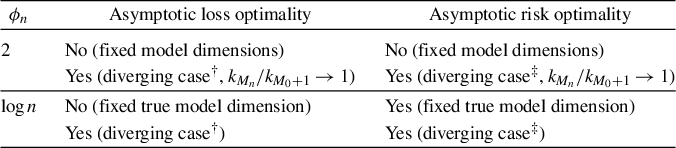
We summarize the main theoretical results in Table 1. One remarkable result is that when $\phi _n=\log n$ and the true model dimension is fixed, the asymptotic loss optimality does not hold, while the asymptotic risk optimality does. This occurs because when the true model dimension is fixed, the true model is not asymptotically loss optimal but is asymptotically risk optimal. This result does not contradict the corresponding finding of Fang et al. (Reference Fang, Yuan and Tian2023), where they demonstrated the asymptotic loss optimality with a fixed true model dimension when $\phi _n=\log n$ , since their result is confined to the special weight set $\mathcal {H}_n^{\delta }$ .

Table 1

Summary of the asymptotic loss and risk optimality for least squares model averaging when the true model is among the candidate models

Table 1 Long description

The table consists of three columns: phi sub n, Asymptotic loss optimality, and Asymptotic risk optimality.

* Row 1: phi sub n is 2. Asymptotic loss optimality is No (fixed model dimensions). Asymptotic risk optimality is No (fixed model dimensions).

* Row 2: phi sub n is 2 (continued). Asymptotic loss optimality is Yes (diverging case dagger, k sub M sub n / k sub M sub 0 + 1 approaches 1). Asymptotic risk optimality is Yes (diverging case double dagger, k sub M sub n / k sub M sub 0 + 1 approaches 1).

* Row 3: phi sub n is log n. Asymptotic loss optimality is No (fixed true model dimension). Asymptotic risk optimality is Yes (fixed true model dimension).

* Row 4: phi sub n is log n (continued). Asymptotic loss optimality is Yes (diverging case dagger). Asymptotic risk optimality is Yes (diverging case double dagger).

Footnotes define the conditions for the symbols:

* Dagger: k sub M sub 0 + 1 approaches infinity, phi sub n squared (k sub M sub 0 + 1 minus k sub 1) / (n eta sub n) approaches 0, and M sub 0 / (k sub M sub 0 + 1 eta sub n) approaches 0.

* Double dagger: k sub M sub 0 + 1 approaches infinity and phi sub n squared (k sub M sub 0 + 1 minus k sub 1) / (n eta sub n squared) approaches 0.

$^\dagger $ : $k_{M_0+1}\to \infty $ , $\phi _n^2(k_{M_0+1}-k_1)/(n\eta _n)\to 0$ , and $M_0/(k_{M_0+1}\eta _n)\to 0$ .

$^\ddagger $ : $k_{M_0+1}\to \infty $ and $\phi _n^2 (k_{M_0+1}-k_1)/(n\eta _n^2)\to 0$ .

From Table 1, we can observe three cases where the asymptotic loss or risk optimality does not hold. These can be attributed to one or both of the following main reasons:

1. (R1) The true model is not asymptotically loss optimal.

2. (R2) Least squares model averaging assigns weights to the over-fitted models with a positive probability.

Specifically, when model dimensions are fixed, MMA is not asymptotically loss optimal due to both Reasons (R1) and (R2), and it is also not asymptotically risk optimal because of Reason (R2). When the true model dimension is fixed, the asymptotic loss optimality of PMA does not hold due to Reason (R1).

When the true model dimension diverges, PMA is asymptotically both loss and risk optimal under certain conditions on $M_0$ , $k_{M_0+1}$ , and $\eta _n$ . This can be attributed to the asymptotic loss and risk optimality of the true model, along with the model averaging method assigning all the weights to the true model. In the case where the true model dimension diverges, MMA is asymptotically both loss and risk optimal under certain conditions. This result is mainly attributed to the condition that $k_{M_n}/k_{M_0+1}\to 1$ , rendering the over-fitted models asymptotically negligible, although MMA may assign weights to them with a positive probability.

In Section S.3.4 of the Supplementary Material, we compare the conditions for asymptotic loss optimality of MMA with those in Peng et al. (Reference Peng, Li and Yang2025) when the true model dimension diverges. In Section S.3.5 of the Supplementary Material, we compare model selection and model averaging in terms of risk when the true model is included.

5 SIMULATION STUDY

In this section, we conduct a simulation study to illustrate the theoretical results presented in Section 4. For each $i=1,\ldots ,n$ , we generate $y_i$ from the model (2.1), where the covariates $(x_{i1}, x_{i2}, \ldots )$ are i.i.d. normal random vectors with zero mean and a covariance matrix whose $(k, l)$ th element is $\rho ^{|k-l|}$ . The random errors $e_i$ are i.i.d. from $N(0, \sigma ^2)$ and independent of $x_{ij}$ ’s. The population R-squared is denoted as $R^2=\mathrm {Var}(\mu _i)/\mathrm {Var}(y_i)$ , which is controlled in the range of $\{0.05, 0.1, 0.5, 0.9\}$ via the parameter $\sigma ^2$ . We focus on the case where the true model has a fixed dimension. Specifically, we set $\rho =0.5$ , $(\beta _1,\ldots ,\beta _5)=(1, -2, 3, 1.5, 4)$ , and $\beta _j=0$ for all $j\geq 6$ . We consider $\mathbf {K}=(1,\ldots ,11)^{\top }$ . Then, $M_n=11$ , $M_0=4$ , $k_{M_0+1}=5$ , and there are six over-fitted models. The sample size n varies with 100, 1,000, 10,000, and 50,000. For each configuration, the simulation is repeated 10,000 times.

We consider least squares model averaging methods with $\phi _n=2$ and $\phi _n=\log n$ . To assess the results in Lemma 1 and Theorem 1, we calculate the averages of $L_n(\mathbf {w}_{M_0+1}^0)/\inf _{\mathbf {w}\in \mathcal {H}_n} L_n(\mathbf {w})$ and $L_n(\widehat {\mathbf {w}})/\inf _{\mathbf {w}\in \mathcal {H}_n} L_n(\mathbf {w})$ . Similarly, to evaluate the results in Lemma 2 and Theorem 2, we calculate the averages of $R_n(\mathbf {w}_{M_0+1}^0)/\inf _{\mathbf {w}\in \mathcal {H}_n} R_n(\mathbf {w})$ and $R_n(\widehat {\mathbf {w}})/\inf _{\mathbf {w}\in \mathcal {H}_n} R_n(\mathbf {w})$ . To facilitate the computation of $R_n(\mathbf {w})$ , we rewrite it as $R_n(\mathbf {w})=\mathbf {w}^{\top } \mathbf {S}_n\mathbf {w}$ , where $\mathbf {S}_n$ is an $M_n\times M_n$ matrix whose $(m, l)$ th entry is $\boldsymbol {\mu }^{\top }(\mathbf {I}_n-\mathbf {P}_{\max \{m, l\}})\boldsymbol {\mu }+\sigma ^2 k_{\min \{m, l\}}$ . 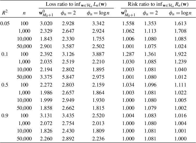Table 2 presents the loss and risk ratios, which are summarized as follows.

Table 2

Simulation results for the loss and risk ratios

Table 2 Long description

The table is organized into eight columns. The first column is R super 2, followed by n, then three columns under the header Loss ratio to infimum of w in H sub n L sub n (w), and three columns under the header Risk ratio to infimum of w in H sub n R sub n (w). The sub-headers for both the loss and risk ratio sections are w sub M sub 0 plus 1 super 0, phi sub n = 2, and phi sub n = log n.

Data is grouped by R super 2 values:

* For R super 2 = 0.05:

- n = 100: Loss ratios are 3.020, 2.928, 3.342; Risk ratios are 1.558, 1.353, 1.613.

- n = 1,000: Loss ratios are 2.329, 2.647, 2.924; Risk ratios are 1.062, 1.113, 1.708.

- n = 10,000: Loss ratios are 1.843, 2.330, 1.755; Risk ratios are 1.006, 1.080, 1.085.

- n = 50,000: Loss ratios are 2.901, 3.587, 2.502; Risk ratios are 1.001, 1.075, 1.024.

* For R super 2 = 0.1:

- n = 100: Loss ratios are 2.392, 3.126, 3.887; Risk ratios are 1.287, 1.361, 1.922.

- n = 1,000: Loss ratios are 2.035, 2.519, 2.210; Risk ratios are 1.030, 1.085, 1.239.

- n = 10,000: Loss ratios are 2.194, 2.802, 1.895; Risk ratios are 1.003, 1.081, 1.040.

- n = 50,000: Loss ratios are 3.375, 5.847, 2.975; Risk ratios are 1.001, 1.080, 1.012.

* For R super 2 = 0.5:

- n = 100: Loss ratios are 2.272, 2.803, 2.159; Risk ratios are 1.034, 1.096, 1.111.

- n = 1,000: Loss ratios are 1.986, 2.657, 1.864; Risk ratios are 1.003, 1.081, 1.022.

- n = 10,000: Loss ratios are 1.999, 2.949, 1.930; Risk ratios are 1.000, 1.080, 1.005.

- n = 50,000: Loss ratios are 1.858, 2.662, 1.815; Risk ratios are 1.000, 1.079, 1.002.

* For R super 2 = 0.9:

- n = 100: Loss ratios are 3.131, 3.435, 2.520; Risk ratios are 1.004, 1.083, 1.016.

- n = 1,000: Loss ratios are 2.072, 2.754, 2.013; Risk ratios are 1.000, 1.080, 1.004.

- n = 10,000: Loss ratios are 1.826, 2.430, 1.809; Risk ratios are 1.000, 1.081, 1.001.

- n = 50,000: Loss ratios are 2.260, 2.892, 2.236; Risk ratios are 1.000, 1.081, 1.000.

First, for each $R^2$ , the risk ratio for the true model converges to 1, while the loss ratio does not. This indicates that the asymptotic loss optimality of the true model does not hold, but its asymptotic risk optimality does, confirming Lemmas 1(i) and 2. Second, for each $R^2$ , the loss ratio for $\widehat {\mathbf {w}}$ with $\phi _n=\log n$ is larger than 1.5 even for large sample sizes, and the risk ratio converges to 1. This means that PMA is not asymptotically loss optimal but is asymptotically risk optimal, confirming the first part of Theorems 1(i) and 2(i). Finally, for each $R^2$ , the loss ratio for $\widehat {\mathbf {w}}$ with $\phi _n=2$ is larger than 2 even for large sample sizes, and the risk ratio stabilizes near $1.08$ . This implies that MMA is not neither asymptotically loss optimal nor asymptotically risk optimal, coinciding with the first part of Theorem 1(ii) and the first part of Theorem 2(ii).

We also conduct additional simulation studies for diverging true model dimensions. To save space, these results are presented in Section S.4 of the Supplementary Material.

6 CONCLUDING REMARKS

In this article, we investigate the asymptotic optimality of least squares model averaging under the weight set $\mathcal {H}_n$ for nested candidate models in the scenario where the true model is included in the set of candidate models. In contrast to Fang et al. (Reference Fang, Yuan and Tian2023), our work is not confined to their special weight set $\mathcal {H}_n^{\delta }$ , and we also explore the asymptotic risk optimality. The main results can be summarized as follows. First, MMA with fixed model dimensions is neither asymptotically loss optimal nor asymptotically risk optimal. Second, when the true model dimension diverges, MMA is asymptotically both loss and risk optimal under $k_{M_n}/k_{M_0+1}\to 1$ and additional conditions on $M_0$ , $k_{M_0+1}$ , and $\eta _n$ . Third, when the true model dimension is fixed, PMA is asymptotically risk optimal but not asymptotically loss optimal. Finally, when the true model dimension diverges, PMA is asymptotically both loss and risk optimal under certain conditions on $M_0$ , $k_{M_0+1}$ , and $\eta _n$ .

These results yield two important insights. First, we show that PMA is not asymptotically loss optimal when the true model dimension is fixed, which differs from the corresponding result of Fang et al. (Reference Fang, Yuan and Tian2023) and from the asymptotic behavior of BIC. This discrepancy arises because asymptotic loss optimality of the true model does not hold under the usual weight set, while it does hold under the restricted weight sets $\mathcal {H}_n^{\delta }$ and $\mathcal {H}_n(N)$ . This finding further indicates that using the discrete weight set of Hansen (Reference Hansen2007) versus the usual weight set for model averaging can result in different asymptotic properties. Second, in the existing model averaging literature, such as Wan et al. (Reference Wan, Zhang and Zou2010), Zhang et al. (Reference Zhang, Zou, Liang and Carroll2020), Zhang (Reference Zhang2021), and Peng et al. (Reference Peng, Li and Yang2025), asymptotic loss optimality and asymptotic risk optimality typically considered as equivalent, but the third result above reveals that these two types of asymptotic optimality are intrinsically different.

In conclusion, we present several interesting directions for future research. First, the results in Lemma 1(i) and the first part of Theorem 1(i) were derived under the assumption of a fixed true model dimension. It remains an open question whether these results still hold in the case of a diverging true model dimension. Therefore, an appealing direction to relax the conditions of the results in this article. Second, it is of interest to investigate the asymptotic optimality of jackknife model averaging (Hansen and Racine, Reference Hansen and Racine2012) in the scenario of this article under heteroskedastic errors. Third, our current results are confined to nested models. It is desirable to extend the analysis to include non-nested models, but it is quite challenging as previously mentioned by Zhang and Liu (Reference Zhang and Liu2019) and Fang et al. (Reference Fang, Yuan and Tian2023). Finally, it would be intriguing to explore similar issues in the context of other models, such as generalized linear models (Zhang et al., Reference Zhang, Yu, Zou and Liang2016), quantile regression models (Lu and Su, Reference Lu and Su2015), and time-series models (Liao et al., Reference Liao, Zou, Gao and Zhang2021).