Introduction
The South Pole station is located on the central high latitude (∼ 3000 m) polar plateau, which is sufficiently inland to avoid the influence of short-lived chemical species that originate from the marine environment. Given Antarctica's huge separation from pollution sources, it was expected to be pristine with very low photochemical activity - an example for clean air conditions (Crawford et al. Reference Crawford2001). Given this expectation, it was assumed that concentrations of trace gases (e.g. NOx (NO + NO2), hydrocarbons, HOx, O3, HNO3 etc.) were low. On the contrary, a series of field campaigns have revealed intense chemical activity as implied by unexpectedly high concentrations of trace gases (e.g. Davis et al. Reference Davis2001), occurring within the Antarctic Boundary Layer (ABL), most notably at the South Pole. The geographical position and meteorology of the South Pole also contributes to this unique chemistry, rather than direct anthropogenic pollution. The low average temperatures during springtime and summertime, ∼ 223 and ∼ 243 K, respectively, frequently cause temperature inversions at the surface, thus limiting the depth of mixed air and greatly impacting boundary layer chemistry. Compounding this issue, the prevailing wind upon the plateau, down-slope off the continent towards the sea, results in longer plateau residence times for air masses. Thus far, the following chemistry has been discovered: 1) NOx associated with high ozone (O3) and NOy (Crawford et al. Reference Crawford2001, Davis et al. Reference Davis2001, Reference Davis, Chen, Buhr, Crawford, Lenschow, Lefer, Shetter, Eisele, Mauldin and Hogan2004, Reference Davis2008, Dibb et al. Reference Dibb, Huey, Slusher and Tanner2004, Huey et al. Reference Huey2004), 2) higher than expected HOx (Chen et al. Reference Chen2004, Mauldin et al. Reference Mauldin, Kosciuch, Henry, Eisele, Shetter, Lefer, Chen, Davis, Huey and Tanner2004), and 3) emissions of formaldehyde (HCHO) and hydrogen peroxide (H2O2) from the South Pole snowpack (Hutterli et al. Reference Hutterli, McConnell, Chen, Bales, Davis and Lenschow2004). These measurements have shown that the South Pole boundary layer can be a highly oxidizing environment. The ABL depth has a strong influence on the photochemical activity present as this governs the mixing volume and, therefore, the impact emissions will have on overlying boundary layer chemistry (Davis et al. Reference Davis2008).
One of the most intriguing aspects of these field campaigns is the high NO (e.g. maximum emission rates of 600 pptvs-1∼ 1.70x10¹⁰ molecules cm-3 s-1) found in the summer at the South Pole (Davis et al. Reference Davis2001), which would normally be associated with suburban pollution. Field studies have shown that nitrate photochemistry at the Arctic and coastal Antarctic snowpack predominantly governs the release of NOx to the overlying boundary layer, reaching levels up to ∼ 200 pptvs-1∼ 5.70x10⁹ molecules cm-3 s-1 (Grannas et al. Reference Grannas2007). In addition, laboratory studies have shown that the photolysis of μM NO3- (2 and 30 μM NO3--doped ice films) on ice produces at most 100 pptv s-1 ∼ 2.80x10⁹ molecules cm-3 s-1 and ∼ 240 pptvs-1 ∼ 6.80x10⁹ molecules cm-3 s-1 of NO2, respectively (Cotter et al. Reference Cotter, Jones, Wolff and Bauguitte2003, Boxe et al. Reference Boxe, Colussi, Hoffmann, Tan, Mastromarino, Case, Sandholm and Davis2003, Reference Boxe2005). Nitric oxide (NO) production solely from nitrate photochemistry at the South Pole on snow/ice does not account for 600 pptv s-1 ∼ 1.70x10¹⁰ molecules cm-3 s-1 of NO (Davis et al. Reference Davis2001). It appears that photochemistry and the changing boundary layer height (BLH) contribute to trace gas emissions at the South Pole. Two campaigns have shown that the photochemistry at the South Pole is being driven by the emission of NOx from the snowpack and the changing BLH (Crawford et al. Reference Crawford2001, Davis et al. Reference Davis, Chen, Buhr, Crawford, Lenschow, Lefer, Shetter, Eisele, Mauldin and Hogan2004), which in turn determines the concentration of NOx by altering the mixing volume. A shallower ABL means a smaller mixing volume, therefore, NOx emissions will produce higher resultant NOx concentrations (Davis et al. Reference Davis, Chen, Buhr, Crawford, Lenschow, Lefer, Shetter, Eisele, Mauldin and Hogan2004). In addition, the 24 hour sunlight exposure of the plateau in conjunction with the enhanced photon flux, due to the high surface albedo, plays an important role in determining the photochemical activity (Lefer et al. Reference Lefer, Hall, Cinquini and Shetter2001, Jones & Wolff Reference Jones and Wolff2003). The concentration of trace gases in the ABL is also affected by the emissions of HCHO, H2O2, oxygenated volatile organic compounds (OVOCs) from the snowpack (Hutterli et al. Reference Hutterli, McConnell, Chen, Bales, Davis and Lenschow2004, Frey et al. Reference Frey, Stewart, McConnell and Bales2005), which have been shown through modelling studies to enhance the HOx budget (Chen et al. Reference Chen2004) and impact ozone production and OH sequestration. Simultaneously, OVOCs can be HOx sinks, depending upon environmental conditions. For instance, Hamer et al. (Reference Hamer, Shallcross and Frey2007) showed that up to 3–4 ppbv of the observed ozone results from the oxidation of OVOCs by OH. In addition, the low average temperatures lead to temperature inversions at the surface, thus limiting the depth of mixed air and greatly impacting overlying boundary layer chemistry. Air masses tend to have long plateau residence times, which are due to the prevailing wind upon the plateau, down-slope off the continent towards the sea.
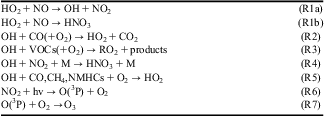
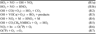
It is well known that HO2 + NO → OH + NO2 (R1a) (Table I) plays a major role in atmospheric chemistry. Recently, HO2 + NO → HNO3 (R1b) (Table I) was discovered in the laboratory (Butkovskaya et al. Reference Butkovskaya, Kukui, Pouvelse and Le Bras2005, Reference Butkovskaya, Kukui and Le Bras2007) and subsequently investigated using the GEOS-CHEM 3-D tropospheric chemical transport model (CTM) (Cariolle et al. Reference Cariolle, Evans, Chipperfield, Butkovskaya, Kukui and Le Bras2008). The Cariolle et al. (Reference Cariolle, Evans, Chipperfield, Butkovskaya, Kukui and Le Bras2008) study was performed at a global scale with a representation of the atmospheric chemistry mostly for the free troposphere. Therefore, the impact could be different for specific regions, where background species concentrations vary from the mean values produced by GEOS-CHEM. This could be the case in boundary layers, over continents or polluted areas. One specific example is in Antarctica, where GEOS-CHEM specifically lacks any parameterization for the modelling of snowpack NOx emissions. Hence, given the need for additional snowpack-polar boundary layer chemical modelling (Jacobi & Hilker Reference Jacobi and Hilker2007, Boxe & Saiz-Lopez Reference Boxe and Saiz-Lopez2008, Reference Boxe and Saiz-Lopez2009, Bock & Jacobi Reference Bock and Jacobi2010) and given the potentially significant impact on regional-scale boundary layer chemistry, we investigate, via a photochemical box model, the impact of (R1b) on NOx, HOx, HNO3, and O3 concentrations just above the South Pole snowpack.
List of all reactions.
Model description
The same photochemical box model used in Hamer et al. (Reference Hamer, Shallcross and Frey2007, Reference Hamer, Shallcross, Yabushita and Kawasaki2008) was used in the present investigation. This photochemical box model was built using ASAD (‘A Self-contained Atmospheric chemistry coDe’, Carver et al. Reference Carver, Brown and Wild1997) and was set up to describe the South Pole boundary layer conditions. The model consists of two vertically stacked boxes of air that mix at a rate such that 10% of the box volume is exchanged with a time step of  h. The upper layer of the model mixes with the free tropospheric background concentrations of long-lived species at a rate of 5% per model
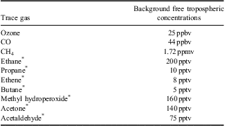
 h time step. The model mechanism has 472 gas phase reactions, representative of 163 species and is based on the Master Chemical Mechanism (Jenkin et al. Reference Jenkin, Saunders and Philling1997). The mechanism includes inorganic reactions, initial reactions of non-methane hydrocarbons (NMHCs) with OH, NO3, and O3, and detailed chemical mechanisms describing the degradation pathways of NMHCs containing up to five carbon atoms. The free tropospheric background concentrations of CO, CH4, and NMHC were adjusted to be consistent with their respective measured background concentrations at Antarctica. The model achieves these concentrations via free tropospheric mixing in the upper box. Non-methane hydrocarbon concentrations and other background species used in the model were obtained from the ISCAT 2000 (Investigation of Sulfur Chemistry in Antarctic Troposphere) campaign and the CHABLIS (Chemistry of the Antarctic Boundary Layer and the Interface with Snow) project. CO and CH4 concentrations were obtained from National Oceanic and Atmospheric Administration South Pole flask data. Given the recent identification of OVOCs (methyl hydroperoxide, acetaldehyde, and acetone) at the South Pole (Frey et al. Reference Frey, Stewart, McConnell and Bales2005, Hamer et al. Reference Hamer, Shallcross and Frey2007), their corresponding background concentrations were also added, such that there is a flux of OVOCs into the upper box. All of the free tropospheric background concentrations are specified in Table II. The albedo of the snowpack surface in the model was set at 0.8 (Lefer et al. Reference Lefer, Hall, Cinquini and Shetter2001). Nitrate photolysis and NOx emissions from the snowpack was described by using a prescribed emission ratio of 1:2 for NO with respect to NO2 (Jones et al. Reference Jones, Weller, Wolff and Jacobi2000, Reference Jones2001, Cotter et al. Reference Cotter, Jones, Wolff and Bauguitte2003). This reflects studies of snowpack concentrations of NOx observed during field campaigns at the South Pole and Neumayer (Crawford et al. Reference Crawford2001, Davis et al. Reference Davis, Chen, Buhr, Crawford, Lenschow, Lefer, Shetter, Eisele, Mauldin and Hogan2004). The flux of NOx out of the snowpack is 2.4 x 10¹⁰ molecules cm-2 s-1. In addition to the snowpack NOx emissions, fluxes of O(3P) atoms were included into the lower box in line with Hamer et al. (Reference Hamer, Shallcross, Yabushita and Kawasaki2008) and Yabushita et al. (Reference Yabushita, Kawanaka, Kawasaki, Hamer and Shallcross2007). HCHO and H2O2 fluxes were added to the model, which were equivalent to their respective fluxes observed at the South Pole (Hutterli et al. Reference Hutterli, McConnell, Chen, Bales, Davis and Lenschow2004). A wide range of chemical species are also deposited in the lower box onto the snow. A complete list of the deposited species and the deposition rates used is included in the supplemental material (M. King, personal communication 2004; http://dx.doi.org/10.1017/S0954102012000144).
Background concentrations used in the model.
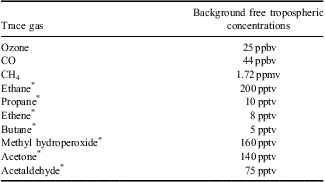
Ppbv = parts per billion by volume, ppmv = parts per million by volume, pptv = parts per trillion by volume.
*Background concentrations of shorter-lived species are higher than reported for ambient South Pole boundary layer levels. The highly oxidizing nature of the South Pole boundary layer requires that free tropospheric concentrations must be elevated relative to the boundary layer concentrations to maintain the observed ambient boundary layer concentrations.
Model simulations
In all of the simulations the model was run over a 15 day period using the same calendar day (30 December) in order to achieve steady state. All of the results presented represent model values from the 15th day though the model does achieve steady state by the 10th day of the simulation. Initial model concentrations of long-lived species are fixed at their background concentrations for the South Pole site and are maintained in part by the downward fluxes due to the free tropospheric background concentrations presented in Table II. These downward fluxes are sufficient to maintain these long-lived species at their observed concentrations. The spin-up period is sufficiently long to prevent model result sensitivity to short-lived species concentrations. A sensitivity analysis was carried out, where the model was setup to run under two scenarios, using the kinetic rate coefficient data for reaction (R1b). The model was run 15 times using a range of BLHs (500, 400, 350, 300, 250, 200, 150, 125, 100, 75, 60, 50, 40, 35 and 30 m) with a constant NOx emission of 2.4 x 10¹⁰ molecules cm-2 s-1. The model produces a range of NOx concentrations that are consistent with observed ranges. Using this full range of tropospheric BLHs, the model was run using a branching ratio (β) of zero for the ‘Base Case’ and using β ∼ 0.78 equivalent to 243 K and surface pressure at the South Pole for the perturbed case, run ‘β-Rate 1’. To be consistent with the central Antarctic plateau region, the location of the box model was set to the surface at 88°S. This location has a weak diurnal cycle in actinic flux, which is not fully representative of the South Pole, but allows for more stable simulations. Further details of the ‘Base Case’ model run can be found in Hamer et al. (Reference Hamer, Shallcross and Frey2007) under ‘run B’ and in Hamer et al. (Reference Hamer, Shallcross, Yabushita and Kawasaki2008) in relation to the ‘1 x O(3P) run’.
Reaction (R1a) plays a central role in atmospheric chemistry by way of OH/HO2 recycling, reduction of ozone depletion by HOx cycles in the stratosphere, and in ozone production in the troposphere. In the stratosphere this reaction moderates the effectiveness of the cycle involving HOx radicals, which is an important removal mechanism of ozone (Wayne Reference Wayne2000). In the troposphere this reaction plays a key role in controlling the interconversion between HO2 and OH radicals through cycles involving OH, CO, and volatile organic compounds (VOCs) (see (R2) and (R3) Table I). The VOCs include methane, NMHCs, and other volatile carbon-containing species. Reaction (R3) is a secondary source of OH radicals as well as the major source of tropospheric ozone, through the conversion of NO and NO2, followed by the photolysis of NO2 to NO and O(3P) atoms. The O(3P) atoms produced combine with O2 to produce ozone. The OH and O3 production rates are, therefore, limited primarily by the chain termination reaction involving OH and NO2 (see Table I for (R4)).
Reaction (R1b) could be another significant chain termination reaction. To assess the importance of reaction (R1b) in the troposphere, Butkovskaya et al. (Reference Butkovskaya, Kukui and Le Bras2007) determined the branching ratio β(T, P) or rate constant ratio, β(T, P) = k 1b/k 1a = (530/T(K)) + (6.4 x 10⁻⁴ x P(torr)) – 1.73, over the full range of tropospheric pressures and temperatures (i.e. 298 K and 760 torr (Earth's surface) to 220 K and 200 torr (Earth's tropopause)). Consequently, at the Earth's surface β(T, P) ≈ 0.5% and in the tropopause region β(T, P) ≈ 0.8%. Given the significant branching of (R1b) (i.e. β(T, P) ≈ 0.78%, for T = 243 K) at the surface in the central Antarctic plateau region, we conduct photochemical box model simulations with and without the inclusion of (R1b) and assess its impact on NOx, HOx, HNO3, and O3 concentrations just above the South Pole snowpack. The rate constant k 1b was derived from β(T, P) by considering the recommended value k 1a = 3.5 x 10⁻¹² exp(250/T) cm3 molecule-1 s-1 (Sander et al. Reference Sander2006). This NASA Jet Propulsion Laboratory evaluation panel recommended value and the one recommended by the International Union of Pure and Applied Chemistry (IUPAC) panel (Atkinson et al. Reference Atkinson, Baulch, Cox, Crowley, Hampson, Hynes, Jenkin, Rossi and Troe2004, updated in 2006 at http://www.iupac-kinetic.ch.cam.ac.uk, accessed June 2006) are very similar, the IUPAC one being higher by only 14% at 200 K and 10% at 300 K.
Results and discussion
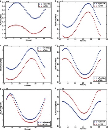
Figure 1a–f displays diurnal photochemical box model simulations at 243 K (representative of the South Pole summer conditions and a BLH of 35 m) of O3, NO, NO2, OH, HO2, and HNO3 with and without (R1b) starting at midday. The blue profiles denote model simulations without (R1b) included, while the red profiles denote model simulations with (R1b) included. Box model simulations show that O3 concentration diurnal profiles follow a typical pattern of variability for a polluted environment at the surface, i.e. ozone production beginning in the morning, followed by a peak in ozone concentrations in mid-afternoon, concluding with a decrease in ozone concentrations during the evening. In this simulation this occurs primarily due to the variability in actinic flux and its direct effects upon the chemistry due to the induced changes in snowpack NOx emissions and photolysis rates of photochemical species. Specifically, increased levels of sunlight lead to enhancements in ozone via reactions (R1a), (R5), (R6) and (R7) (Table I). The decrease in ozone occurs in the evening as the ozone production rate decreases to a point where the combined loss rate for ozone due to deposition and the reaction of O3 and NO are faster. Ozone production decreases as the levels of HOx and RO2 radicals diminish. Including (R1b) causes the net sink of HO2 and NO to increase and, consequently, the ozone production rate is decreased, leading to decreased ozone concentrations throughout the entire day. HNO3 follows a similar profile to HOx species at high NOx values (i.e. [NOx] > ∼ 300 pptv), reduced HOx and NO2 concentrations, which results in a decrease in production rate of HNO3.
Diurnal photochemical box model simulations, representative of South Pole conditions of a. O3, b. NO, c. NO2, d. OH, e. HO2, and f. HNO3 with (red lines) and without (blue lines) HO2 + NO → HNO3 (R1b). All model simulations start at midday. Note: in this figure (k1b) refers to the reaction rate constant of (R1b), which in turn, refers to the same reaction.

The inclusion of (R1b) decreases O3, NO, NO2, and OH by 3 ppbv, 200 pptv, 125 pptv, and 0.3 pptv, respectively, from their simulated peak concentrations, while HNO3 increases by 125 pptv from its peak simulated concentration. Although the peak concentration of HO2 is unaffected by the new chemistry, a small decrease in the lower limit HO2 is simulated, which is due to the increased efficiency of the HO2 + NO → HNO3 production channel at colder temperatures. Ozone concentrations have reached as high as ∼ 45 ppbv during the summer at the South Pole (Crawford et al. Reference Crawford2001). The new reaction decreases peak ozone concentrations from ∼ 37–34 ppbv, thus worsening the agreement with observations of maximum ozone concentrations at the South Pole. Reaction (R1b) brings better agreement with the peak NO amounts (600 pptv) measured (Davis et al. Reference Davis2001, Reference Davis, Chen, Buhr, Crawford, Lenschow, Lefer, Shetter, Eisele, Mauldin and Hogan2004) during summertime at the South Pole by decreasing peak NO concentrations from ∼ 950 to ∼ 750 pptv (Hamer et al. Reference Hamer, Shallcross and Frey2007, Reference Hamer, Shallcross, Yabushita and Kawasaki2008). The new reaction reduces NO2 concentrations from 525–400 pptv. Matsuki et al. (Reference Matsuki, Yoshikawa, Yanagisawa and Kasuga2002) provided the only ambient measurements of NO2 at the South Pole and measure a peak NO2 concentration of 2.8 ppbv. OH is brought into better agreement with observations (i.e. mean concentrations at the South Pole of 0.09 pptv (2.5 x 10⁶ molecules cm-3)) (Mauldin et al. Reference Mauldin, Kosciuch, Henry, Eisele, Shetter, Lefer, Chen, Davis, Huey and Tanner2004). With (R1b) included the mean OH concentration is reduced from ∼ 1.10–0.40 pptv (∼ 3 x 10⁷ molecules cm-3 to ∼ 1 x 10⁷ molecules cm-3), which brings our model simulations into better agreement with measured OH in the ABL. A substantial discrepancy remains, however, and this may be due in part to the absence modelled of loss of HOx due to reaction with NOx within the snowpack (Hamer et al. Reference Hamer, Shallcross and Frey2007). Given that the peak HNO3 concentrations measured at the South Pole is ∼ 70 pptv (Huey et al. Reference Huey2004), our photochemical box model simulations still over predict the HNO3 by an additional 125 pptv. Yet, modelled HNO3 concentrations and observation agreement may not represent the best test of the new reaction channel since HNO3 was substantially overestimated before the introduction of (R1b). This overestimation is probably due to the model over predicting HOx concentrations. HO2 simulations are incongruent with maximum and mean concentrations of HO2 measured at the South Pole, ∼ 2.50 pptv to 0.04 pptv (∼ 7 x 10⁷ and ∼ 1 x 10⁶ molecules cm-3), respectively (Chen et al. Reference Chen2001).
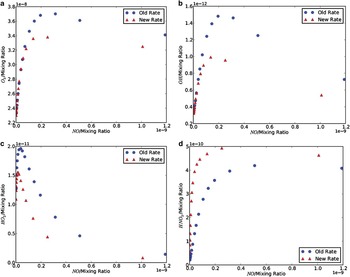
Figure 2 displays box model simulations of the mixing ratio dependence of O3, OH, HO2, and HNO3 on the BLH (ranging from 30–500 m, where smaller BLHs lead to elevated NO). Table III displays modelled concentration ranges for select species with and without the new reaction channel compared to observed species concentration ranges. The NO mixing ratios are shown with (red profile) and without (blue profile) the inclusion of reaction (R1b) (Fig. 2). For low concentrations of NO (i.e. < 50 pptv) and high BLHs, ozone increases similarly with NO with and without (R1b) as NO concentrations are not large enough to significantly reduce HO2, despite the extra loss pathway (Fig. 2a). As NO concentrations exceed 100 pptv, (R1b) starts to influence the loss of HO2, which in turn leads to less ozone production. At NO > ∼ 300 pptv, O3 starts to decrease (without (R1b)), while at NO > ∼ 250 pptv O3 starts to decrease (with (R1b)). Both profiles exhibit this behaviour as OH start to decrease because of the decreased production of HOx and NO2. OH follows a similar concentration dependence on NO as O3 (Fig. 2b), which is linked to the decrease in OH at NO > ∼ 100 pptv due to the increased destruction of HO2, via (R1b), and decreasing solar radiation, which in turn, caused the production rate of OH to decrease. OH concentrations (without (R1b)) start to decrease at NO > ∼ 200 pptv, while it decreases (with(R1b)) at NO > ∼ 150 pptv. Figure 2c shows less HO2 with the inclusion of (R1b) as (R1b) represents an extra sink for HO2. HO2 decreases at lower NO concentrations (i.e. at NO > ∼ 40 pptv without (R1b) and at NO > ∼ 20 pptv with (R1b)), compared to O3 (i.e. at NO > ∼ 300 pptv without (R1b) and at NO > ∼ 250 pptv with (R1b)) since the primary pathway leading to the formation of O3 is preceded by the photolysis of NO2, which itself is much larger in concentration than HO2 (e.g. peak NO2 ∼ 500 pptv vs peak HO2 ∼ 5 pptv, see Fig. 1c & e) and is solely not produced from gas phase chemistry but is also emitted readily from the snowpack via nitrate photolysis and diffusion (Hamer et al. Reference Hamer, Shallcross, Yabushita and Kawasaki2008). HNO3 concentrations (without (R1b)) start to decrease at NO > ∼ 500 pptv while it decreases (with (R1b)) at NO > ∼ 250 pptv. HNO3 production is a function of OH and NO2 so (at NO > ∼ 250 pptv) OH and NO2 decrease due to (R1b).
The mixing ratio dependence of a. O3, b. OH, c. HO2, and d. HNO3 on the NO mixing ratio with (red profile) and without (blue profile) the new reaction HO2 + NO → HNO3 (R1b) included. Each data point represents midday concentrations for the individual model run, using different boundary layer heights.

Modelled concentration ranges for select species with and without the new reaction channel compared to observed species concentration ranges. Note that the variability of these species in the model that leads to these ranges is due to the changes in boundary layer height.

*Bracketed range excludes OH values affected by fog events as described by Chen et al. Reference Chen(2001).
Implications
The identification of the new channel for (R1) and its suggested impacts upon the average radical chain length and ozone production at the South Pole present some implications for previously published work regarding this location and for other cold regions of the atmosphere. Estimates of the photochemical lifetime of NOx with respect to (R4) are on the order of 3.5 hours, assuming summertime observed OH concentrations 0.09 pptv (2.5x10⁶ molecules cm-3) (Mauldin et al. Reference Mauldin, Kosciuch, Henry, Eisele, Shetter, Lefer, Chen, Davis, Huey and Tanner2004) and that T = 243 K. The introduction of the new channel reduces the NOx lifetime with respect to oxidation to HNO3 to ∼ 1 hour with the new channel now dominating the conversion of NOx to HNO3 - again utilizing observations of summer HO2 (Mauldin et al. Reference Mauldin, Kosciuch, Henry, Eisele, Shetter, Lefer, Chen, Davis, Huey and Tanner2004). Thus, existing estimates of snowpack NOx emissions relying on previous estimates of NOx lifetime, perhaps, need to be re-evaluated (Wang et al. Reference Wang, Choi, Zeng, Davis, Buhr, Huey and Neff2008). Such a re-evaluation would need to be revised upwards, which presents a problem for NOx flux estimates based upon snow radiative transfer models that tend to underestimate snowpack NOx production rates (Wolff et al. Reference Wolff, Jones, Martin and Grenfell2002, Davis et al. Reference Davis2008) when compared to current observationally derived flux estimates at the South Pole (Oncley et al. Reference Oncley, Buhr, Lenschow, Davis and Semmer2004). This further widens the apparent inconsistency between theoretically required emission burdens at the South Pole, conventional laboratory measurements, and eddy flux covariance estimates of snowpack NOx emissions (Davis et al. Reference Davis2008). In addition, a significant revision of the photochemical lifetime of NOx due to the new channel would generally require other observationally constrained inverse estimates of NOx sources in other environmental regions to be revised. This wider re-evaluation of NOx lifetime due to the new channel would have particular significance for the emission inversion studies in the upper atmosphere, specifically, with regard to lightning and aircraft NOx inverse source estimation (Martin et al. Reference Martin, Sauvage, Folkins, Sioris, Boone, Bernath and Ziemke2007) since these studies rely on the forward model to accurately describe the NOx lifetime.
The model simulations including (R1b) result in a substantial increase in boundary layer HNO3(g), thus over predicting it by over 100 pptv when compared to measurements. This effect would undoubtedly increase surface NO3- concentrations via HNO3(g) deposition. Taking into account an increase in surface NO3- concentrations, via an increase in HNO3(g), would have no effect on HOONO and HONO produced from nitrate photolysis. HOONO is produced from NO3- photodecomposition at λ < 280 nm, via NO3-*, still, NO3-* quickly isomerizes back to NO3- (Boxe Reference Boxe2005). Concomitantly, as OH + NO2 → HOONO (within the solvent cage of ice), it also quickly isomerizes back to NO3- and H+. HONO production was believed to have a substantial source from NO3- photolysis as NO2-, a primary product, at low pH readily protonates to form HONO (or nitrous acid in ice). Given that nitrate photochemistry proceeds via two primary photolytic channels (i.e. 10% branching to produce NO2- + O(3P) and 90% branching to produce NO2 + O-), NO2- concentrations will always be smaller than NO2. For example, snowpack kinetic modelling of nitrate photochemistry by Jacobi & Hilker (Reference Jacobi and Hilker2007) revealed that NO2- concentrations are always lower than NO2 concentrations by a factor of approximately three. They also show that in addition to the difference in NO2- and NO2 concentrations, the transfer rate of HONO produced via NO2- protonation at low pH would limit any release of HONO produced in the snowpack, whether it is sourced from nitrate photolysis or other chemical or photochemical reaction channels. In other words, Jacobi & Hilker (Reference Jacobi and Hilker2007) showed that the high Henry's law constant for HONO at low temperatures (e.g. 930 M atm-1 at -20°C, which is 3.6 x 10⁴ higher than the solubility constant for NO2 at -20°C), dictates its slow transfer from the snowpack to the gas phase.
Conclusions
Here, we examined the effect of the new reaction channel, HO2 + NO → HNO3 (R1b) at the South Pole, Antarctica using a photochemical box model. The inclusion of this reaction decreases O3, NO, NO2, OH, and HO2 and increases HNO3. The decrease in O3 from 37–34 ppbv worsens the agreement between the model and the highest O3 concentrations observed at the South Pole (45 ppbv), which are associated with in situ photochemical production. As the mean concentration of OH at the South Pole is 2.5 x 10⁶ molecules cm-3, our box model simulations brings OH into better agreement with observations since OH is reduced from 1 x 10⁷ to 8 x 10⁶ molecules cm-3. Box model simulations of HO2 are incongruent with maximum and mean concentrations of HO2 measured at the South Pole, ∼ 7 x 10⁷ and ∼ 1 x 10⁶ molecules cm-3, respectively. Given that peak measured HNO3 concentration measured at the South Pole is 70 pptv, our box model simulations still over predict it by an additional ∼ 130 pptv. The reduced concentrations of NOx, as a result of the application of the new channel, are consistent with expected decreases in atmospheric NOx lifetime as a result of increased sequestration of NOx into HNO3. We also show here that without (R1b) current models will overestimate NOx concentrations at the ABL, which has the following implications: 1) given that previous studies investigating snowpack emissions of NOx have relied upon accurate and comprehensive determinations of NOx losses in this environment, our result implies that NOx snowpack emissions are larger than currently reported, 2) current estimates of the nitrate recycling factor again rely upon accurate characterization of NOx, and therefore, current estimates are probably too low, and 3) the changes in NOx lifetime imply that snowpack NOx emissions and snowpack nitrate recycling must be re-evaluated. Further analysis is required to reduce the degree of incongruence. Our box model simulations of the concentration dependence of OH, O3, HO2, and HNO3 on NO with the new reaction included, overall, show a decrease in OH, O3, and HO2 and an increase in HNO3. Lastly, this new reaction should be further explored and validated experimentally for potential consideration and inclusion in the latest ‘Chemical kinetics and photochemical data for use in atmospheric studies evaluation’ handbook.
Acknowledgements
Paul Hamer was supported by an appointment to the NASA Postdoctoral Program at the Jet Propulsion Laboratory, administered by Oak Ridge Associated Universities through a contract with the National Aeronautics and Space Administration (NASA). The work described here was performed at the Jet Propulsion Laboratory, California Institute of Technology, under contracts with NASA. The constructive comments of the reviewers are gratefully acknowledged.
Supplemental material
A Supplemental table will be found at http://dx.doi.org/10.1017/S0954102012000144.