1. Introduction

The probabilistic notion of likelihood offers a systematic means of assessing “the relative merits of rival hypotheses in the light of observational or experimental data that bear upon them” (Edwards Reference Edwards1972, 1). In particular, likelihood allows one to adjudicate among competing hypotheses by way of a two-part principle:

The claims sanctioned by LL are strictly comparative. The principle does not say what you should believe or to what degree you should believe it. Rather, the notion of ‘supporting’ one hypothesis over another is contrastive and perhaps best characterized as a relation of ‘favoring’ (Sober Reference Manson2008). LL tells you how to determine the degree to which one hypothesis is favored over another on the basis of some evidence, E, and nothing more. Proponents of the principle are adamant that LL cannot provide sufficient grounds for apportioning belief, only ranking hypotheses in a particular evidentiary context.

While LL has been defended at length as a general tool for both formal and informal reasoning about hypothesis ranking (see, e.g., Hacking Reference Hacking1965; Edwards Reference Edwards1972; Sober Reference Manson2008), there remains an important ambiguity in its application. Intuitively, we ought to make use of all available information when assessing the relative merits of two hypotheses, not just the particular piece of evidence E under consideration. Any additional information already in our possession before obtaining E is typically referred to as background information. LL does not, on the face of it, tell us how to deal with such information. Some, most prominently Elliott Sober (Reference Sober and Manson2003, Reference Manson2008, Reference Manson2009), have argued that we ought to condition on this additional information when computing likelihoods. That is, if we denote the background information by B, then the likelihood ratio we should use is . Taking this approach, however, means that —and thus our judgments concerning rival hypotheses H ₁ and H ₂—will depend on exactly which information is taken to constitute background information and which is considered evidence and thus part of E. Under Sober’s interpretation, LL can be taken to yield different judgments for the same data when the line between evidence and background information is moved. The use of LL is thus encumbered by a “line-drawing problem” (Kotzen Reference Kotzen2012).

This line-drawing problem also appears in a slightly different guise in the literature on statistical inference. In this more restricted context, the problem manifests as an apparent ambiguity in the likelihood function. Specifically, there appears to be no systematic way of deciding which random variables and model parameters should be included in the likelihood function and no principled way of deciding on which side of the conditionalization bar these quantities belong if included.Footnote ² As in the general case, the problem for the likelihoodist is to provide a principled division of propositions into background and evidence.

A variety of solutions have been proposed to both versions of the problem of background information, although not always in these terms. Some (e.g., Weisberg Reference Weisberg2005) attempt to provide a principled means of distinguishing evidence from background information. Others (e.g., Kotzen Reference Kotzen2012) attempt to dissolve the problem by scrapping or revising LL.Footnote ³ In the context of statistical inference, a common strategy is to disambiguate the likelihood function by fiat (see, e.g., Grossman Reference Grossman, Forster and Bandyopadhyay2011). I argue that none of these strategies is well motivated. Background information is only problematic when one fails to distinguish between two related questions: (i) Given that I know B, to what degree does the additional piece of evidence E support H ₁ over H ₂? And (ii) to what degree does all the evidence at hand—B and E—support H ₁ over H ₂? My aim is to demonstrate that, once these questions are distinguished, the very same considerations that motivate the adoption of LL entail distinct answers to both questions, thus resolving any ambiguity over the treatment of background information. Note that I am emphatically not offering a defense of LL as a general inference procedure. Mine is the more modest goal of dissolving an apparent defect of LL using the resources to which proponents of the principle already assent.

To draw out the distinction relevant to eliminating the problem of background information, I will begin with a detailed example. I then argue for an expression that represents the degree to which a particular piece of evidence supports one hypothesis over another in context, and then I derive a related expression for the total support provided by all available evidence. Finally, I show how these new expressions dissolve ambiguities in the treatment of background information by applying them to the so-called fine-tuning argument.

2. Illustrating the Problem

To draw out the distinction that I claim obviates the problem of background information, it will help to have a concrete example in mind. To avoid preconceived interpretations, I will intentionally eschew standard examples, at least at the outset. So rather than treat of fish or firing squads, I will consider carnivals.

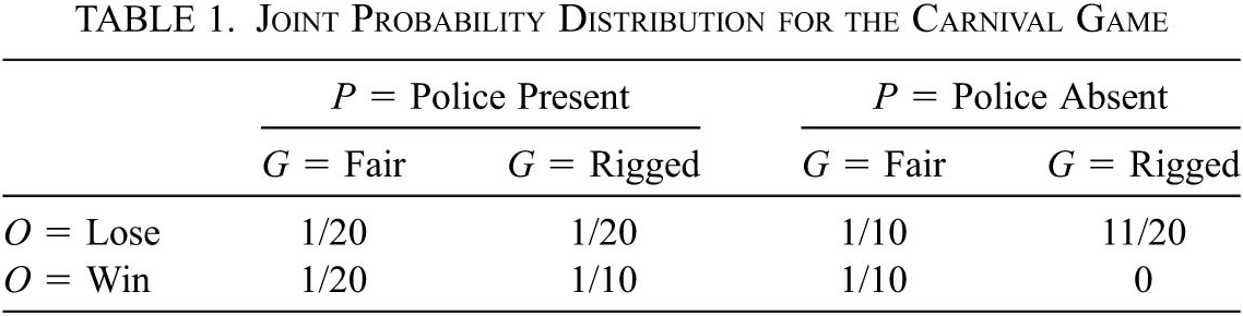
Suppose that Albert finds himself on the midway of an old-fashioned carnival. He decides to play one of the games—the one where contestants try to toss a ball into a milk can. Albert is savvy about carnival games; he knows they are often rigged. In a fair game, there is a 50% chance of winning a prize. But when no authorities are around, there is an appreciable chance that the carnie running the game will hand him a ball too big to fit in the can, making it impossible to win. However, if there happens to be a police officer in sight, the game is likely to be rigged in Albert’s favor—the carnies want the police to think the games are fair, so they arrange to let people win when the authorities are present. A set of probabilities reflecting these facts is provided by the joint distribution of table 1.

Table 1.Joint Probability Distribution for the Carnival Game

	P = Police Present	P = Police Absent
	G = Fair	G = Rigged	G = Fair	G = Rigged
O = Lose	1/20	1/20	1/10	11/20
O = Win	1/20	1/10	1/10	0

Knowing all of the probabilities in table 1, Albert puts his money down and promptly tosses a ball into the can. Given that he has just won, what can Albert conclude about the game? Specifically, does he now have grounds to favor the hypothesis that the game is fair over the hypothesis that it is rigged (i.e., surreptitiously biased either for or against him)? According to LL, Albert needs to compare two probabilities: the probability that he would win given that the game is fair, P(win|fair), and the probability that he would win given that the game is rigged, P(win|rigged). Since P(win|fair) = 1/2 > P(win|rigged) = 1/7, LL asserts that Albert’s success in the game supports the hypothesis of a fair game—Albert has reason to favor the claim that he has played a fair game.

But suppose that, before he tosses the ball, Albert notices a police officer standing near the booth. What can be said in light of this additional information? Here is where different interpretations of LL begin to diverge. According to Sober’s approach, we must recognize two sorts of propositions: evidence and background knowledge. Evidence is whatever fresh information we are currently considering when applying LL to distinguish among hypotheses. It appears to the left of the conditionalization bar when computing a likelihood. Background knowledge constitutes whatever we already know about the world and is presumed to belong on the right side of the conditionalization bar. According to this view then, Albert should treat the fact of the police officer’s presence as background knowledge and condition on this information. The relevant likelihoods are now P(win|fair, present) = 1/2 and P(win|rigged, present) = 2/3. With the additional information, he should now favor the hypothesis that the game is rigged—the background information has reversed our ordering on hypotheses.

That we should take all available information into account when comparing hypotheses is not especially controversial—most authors assume some sort of principle of total evidence (Carnap Reference Carnap1947). What is controversial is how and whether ‘evidence’ should be distinguished from background information. It is not clear why Albert should treat the information that a police officer was present any differently from the information that he won the game. Albert might just as well have treated the observation of the police officer as the evidence and conditioned instead on the fact that he won: P(present|rigged, win) = 1 > P(present|fair, win) = 1/3. In this way of accounting for all the information, LL still favors the hypothesis that the game is rigged but does so to a much greater degree. Alternatively, Albert might have treated all the information at hand as ‘evidence’ and compared the following likelihoods: P(win, present|fair) = 1/6 > P(win, present|rigged) = 1/7. Taking this approach once again inverts the ordering of hypotheses and favors the hypothesis that the game was fair. It might appear then that LL must be modified in order to provide a principled means of discriminating background information from evidence. However, no such modification is required—a careful interpretation of LL as it stands obviates the question of evidence versus background information.

3. The Piecewise Impact of Evidence

To resolve the ambiguity over background information, we need to distinguish between two questions: (i) To what degree does learning a particular fact in the context of an additional set of facts support a given hypothesis? And (ii) to what degree does learning a particular fact in conjunction with an additional set of facts support a given hypothesis? In terms of the midway example above, the distinction can be made as follows: (i) To what degree does winning the game having already learned that a police officer is present support the hypothesis that the game is fair? And (ii) to what degree does the full set of information at hand—that Albert has won the game and that a police officer was present—support the hypothesis that the game is fair?

To address question i, we need to examine the piecewise introduction of evidence, taking care to note one important fact: learning the truth of a proposition (or the value of a random variable) is effectively an intervention that changes the background distribution describing the ways the world might be. To begin with, let us assume that we are given a full joint distribution reflecting all relevant aspects of the world and nothing else—there is nothing given that might qualify as either evidence or background information. For ease of exposition, I further assume that this distribution is discrete, although nothing about my derivation hinges on this being the case.

Since all we have is the distribution and no information to sort out, LL can be applied unambiguously upon obtaining our first piece of evidence, I ₁. According to LL, the degree to which this information supports hypothesis H ₁ over H ₂ is given by the likelihood ratio . Furthermore, on learning that I ₁ is the case, the space of possible events has been reduced—acquiring information requires us to update the background distribution with which we started. Specifically, the probability of I ₁ being the case must now be unity, irrespective of the value it had prior to learning this outcome. One way to represent the change is to construct a new event space by simply removing all the events incompatible with the fact that I ₁ is the case while preserving the relative measure on all remaining events. 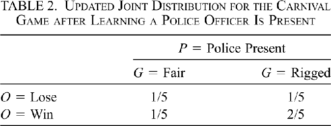That is, the new distribution , where is any event in the original event space compatible with I ₁, is obtained from the old distribution by the following relation: .Footnote ⁴ In the midway example, for instance, when Albert learned that a police officer was present he should have replaced the original distribution of table 1 with that of table 2.

Table 2.Updated Joint Distribution for the Carnival Game after Learning a Police Officer Is Present

	P = Police Present
	G = Fair	G = Rigged
O = Lose	1/5	1/5
O = Win	1/5	2/5

Once we realize that we are working with a new distribution, there is no need to draw a line between background information and evidence—our prior information is reflected in the new distribution. When additional evidence, I ₂, is acquired, we need only appeal to LL just as we did at the outset. This time, however, we are assessing likelihoods with respect to the currently applicable distribution . So the evidence I ₂, if we take LL seriously, supports H ₁ over H ₂ just if P ₁(I ₂|H ₁) > P ₁(I ₂|H ₂) and does so to a degree . In terms of the original joint distribution, we can express this likelihood ratio as .

As before, when we learn I ₂, we must update our distribution to reflect this restriction of the possibilities. This new distribution is obtained from the old distribution in the same way as above: . This is easy to generalize for an indefinite sequence of evidence: once we have learned I ₁, I ₂, … , I _n−1, we should compute the likelihoods involving a new piece of evidence I_n using the distribution . The new piece of information I_n introduced in the context of prior information I ₁, I ₂, … , I _n−1 supports H ₁ over H ₂ just if P(I_n|I _n−1, … , I ₁, H ₁) > P(I_n|I _n−1, … , I ₁, H ₂) and does so to the degree

The point is that whenever we acquire a piece of information we can apply LL without modification, but we must do so using a distribution that reflects all of the facts already in evidence. Put this way, there is no ambiguity in using LL—we always compute a straightforward likelihood. However, when this likelihood is expressed in terms of the original joint distribution with which we started, each successive likelihood is conditioned on the previous facts. So by applying LL and taking care to note the way in which the acquisition of information forces a change in distribution, we have found that in order to determine the relative support of one hypothesis over another provided some particular piece of evidence, we must use likelihoods conditioned on all previously acquired facts.

Thus far, it may seem that I have been arguing for Sober’s interpretation of LL. However, Sober seems to view the likelihood ratio (1) as representing the overall degree to which H ₁ is supported over H ₂ once I_n is obtained. I have been urging that, if we take LL at face value, this is not how we should interpret this expression. At every stage in the above derivation, we were applying LL to determine the degree to which a particular piece of evidence supported one hypothesis over another. Other information was relevant, but only in determining the epistemic context in which this degree of support was determined. I am suggesting that Sober has the right expression but gives it in answer to the wrong question—in what follows, I show that LL leads us to a very different expression for the degree of support for H ₁ over H ₂ provided by the totality of evidence.

4. Total Support

There are two ways to argue for an expression of the likelihood ratio pertaining to the totality of available evidence. In one approach, we could take the expression given in (1) for the degree to which a particular piece of evidence supports H ₁ over H ₂ and couple this with a function for combining likelihood ratios—a function measuring the overall degree to which two pieces of evidence support H ₁ over H ₂. Strictly speaking, this means adding to LL since the principle does not provide such a rule. However, there are some reasonable constraints we can put on such a function without begging the question concerning background information. For starters, whatever function f we choose should itself yield a likelihood ratio, meaning that it must map pairs of likelihoods to the interval [0, ∞). Furthermore, if either likelihood ratio in the combination is zero—implying that one hypothesis has been entirely ruled out—then the joint likelihood ratio should also be zero. The function should be symmetric since it ought not to matter in what order we give the likelihoods to be combined, and it should be an increasing function of both arguments. An obvious choice satisfying all of these constraints is simply the product of the component likelihoods. That is, given and , the combined likelihood is given by . With this rule for combining likelihoods, we can use the results of the last section to derive an expression for the overall degree to which the facts I ₁, I ₂, … , I_n support one hypothesis over another, assuming they were learned in sequence:

Using nothing but the rules of probability, the right-hand side of equation (2) can be written much more compactly to give the following expression for the total support of the facts I ₁, I ₂, … , I_n:

Of course, the right-hand side of equation (3) is just the expression we would have gotten by applying LL to the proposition I ₁ ∧ I ₂ ∧ … ∧ I_n with respect to the initial joint distribution—in a straightforward reading, it is just the total support for H ₁ over H ₂ provided by the conjunction of all available evidence.

The form of equation (3) suggests that it might have been derived more directly by appealing to LL without worrying about how to determine the contextual support provided by each piece of information or introducing a way to combine these (thus justifying my claim that we need not modify LL). All we had to do was note that, if we let E = I ₁ ∧ I ₂ ∧ … ∧ I_n, then LL immediately yields (3). From (3) we could then deduce (2) just from the rules of the probability calculus. Once we identified the factors of the right-hand side of equation (2) with individual likelihood ratios, we could have used this fact to justify a rule for combining likelihoods. In fact, this is what Edwards (Reference Edwards1972) does, at least in the special case of independent evidence, in his development of the likelihood framework. Viewed from this perspective, equation (3) is implicit in LL. Whichever approach we take to justifying this rule for assessing total support, we are led to the following amplified form of LL:

With ALL, we can answer the questions posed above concerning the midway example. The information that Albert has won the game, acquired after learning that a police officer is present, supports the hypothesis that the game is rigged because P(win|present, rigged) > P(win|present, fair). According to ALL ii, this information favors the rigged hypothesis over its rival to a degree . This one piece of information, in the context of previously established information about the presence of police officers, tends to favor the hypothesis of a rigged game. However, the aggregate information—that a police officer is present and Albert has won the game—favors the hypothesis that the game is fair. This follows from ALL iii and iv since . This looks like a contradiction until we realize that the first piece of information obtained—that the police officer is present—strongly favored the hypothesis that the game is fair: P(present|fair)/P(present|rigged) = 14/9. The upshot is that the aggregate effect of the totality of evidence can differ from the piecewise impact of each bit of evidence. Rather than being a contradiction, this is precisely how one would expect these two distinct measures to relate—the total support for the fair hypothesis is simply the product of the contextual likelihood ratios for each piece of evidence.Footnote ⁵

5. Kicking Away the Full Distribution Ladder

In the preceding arguments, I made extensive use of full probability distributions. This appears problematic since the appealing feature of the likelihood approach—and that which sets it apart from Bayesianism—is its disregard for prior probabilities. However, I claim that the likelihoodist who thinks that prior probabilities are often absent or unattainable might nonetheless justify LL or ALL. To see how, let us reconsider the case in which we start with a full prior distribution and then obtain evidence I ₁. Once we acquire the evidence, we should update the probabilities assigned to H ₁ and H ₂ by setting each new probability equal to the corresponding conditional probability assigned by the original distribution:

What can we now say about the degree to which I ₁ favors H ₁ over H ₂? One way we might understand this question is in terms of a hypothetical. Suppose that either H ₁ or H ₂ is true. Then the initial odds in favor of H ₁ are simply P(H ₁|H ₁ ∨ H ₂)/P(∼H ₁|H ₁ ∨ H ₂) = P(H ₁)/P(H ₂). How does the new information change the odds in favor of H ₁? In this case, the posterior odds are given by

The right-hand equality in equation (4) indicates that all of the work to shift the posterior odds up or down relative to our prior odds is being done by the likelihood ratio, . In other words, the change in posterior odds is a function of . To put it still another way, the effect of I ₁ on the odds is entirely determined by .Footnote ⁶ This fact motivates adopting the likelihood function as a measure of relative support. While the likelihood ratio cannot tell us which posterior probability is higher, it can tell us how the odds shift in favor of one hypothesis or the other, assuming that one or the other is right. Furthermore, it does so whether or not we know the prior probabilities. In this sense, LL is a general guide to differential support, and in those cases in which we have no objective basis for assigning priors, the likelihoodist claims it is our only guide.

By considering effects on posterior odds, we can motivate ALL in much the same way as LL. As before, the full distribution (if we knew it to begin with) after learning I ₁ would be given by . If we now learn that I ₂ is the case, then we must change our posterior odds in favor of H ₁ over H ₂ to the following:

Once again, it is the likelihood function that increases (or decreases) the posterior over the prior odds. This time, however, it is in the context of the new distribution , a distribution reflecting prior knowledge of I ₁. If the motivation offered for LL in the first place is compelling, then it seems we must also accept ALL i and ii—the relative support for H ₁ over H ₂ conferred by the new piece of evidence I ₂ after already learning I ₁ is indicated by the likelihood function . But what about the overall support for H ₁ over H ₂ given our epistemic starting point? How should our posterior odds have changed relative to our initial odds as a result of learning I ₁ and I ₂? We can rewrite the right-hand side of equation (5) as follows:

With the posterior odds written this way, we can see that the combined likelihood function determines the change in odds relative to what they were before learning anything at all. So once again, we can kick away the ladder of the full distribution. If we did know the distribution, then learning I ₁ and I ₂ would change the odds in favor of H ₁ over H ₂ by an amount given by the likelihood ratio. Since this is true irrespective of what the priors are, we can always take the likelihood alone to indicate differential support, in this case the degree of support for H ₁ over H ₂ conferred by the totality of evidence.

Of course, one might object to my interpretation of what it is to favor one hypothesis over another. Instead, one might attempt to prove LL i from other premises and take the quantitative measure of contrastive support given by LL ii to be a postulate that stands or falls with how well the results coincide with our intuitions.Footnote ⁷ ALL could then be motivated by the second line of argument I suggested in the previous section: treat all information as evidence and note that the resulting likelihood ratio factors into a product of likelihoods, each of which can be consistently interpreted as corresponding to the impact of a single piece of information.

The point is that insofar as LL is well motivated, so too is ALL. My use of full distributions above was strictly heuristic. Once we have seen what role the likelihood function plays and which likelihood function is relevant to which question, we can ignore the full distribution. Of course, the proponent of LL or ALL can only claim to be free of worrisome priors if conditional probabilities can be taken as primitive.Footnote ⁸ It is not my task here to defend that claim and thus rescue likelihoodism from the charge of subjectivity. My more modest assertion is simply that if we have grounds to take LL seriously, then we should really embrace ALL. Once we have done so, it becomes clear that whatever problems likelihoodism has, line drawing is not one of them.

6. But What Is the Likelihood Function?

My arguments so far have concerned the problem of background information as it appears in the literature on LL in its broadest epistemic use. As I mentioned above, the same problem arises in the more restricted context of statistical inference. Addressing this narrower community, Bayarri et al. (Reference Bayarri, DeGroot, Kadane, Gupta and Berger1988) famously asked, “What is the likelihood function?” To illustrate the ambiguity in answering that question, the authors consider a case analogous to one in which, with respect to each possible value of some discrete parameter characterizing a statistical model, a random variable X has a conditional probability distribution .Footnote ⁹ Furthermore, it is not the random variable X that is observed but rather some other random variable Y for which the conditional distribution is . The authors then ask, “What is the [likelihood function] in this problem?” (6). They claim that there are three candidates, , , and , and that a “subjective judgment must be made in order to decide which of the functions … to use in a given problem” (6). Additional examples in the context of statistical prediction and inference involving unobserved variables are invoked to suggest that the likelihood function is ambiguous in all circumstances. Put differently, no general, rigorous inferential principle has been provided by proponents of likelihood methods that would determine a unique choice of likelihood function for any given problem. According to Bayarri et al., “the reason for this lack is that no general definition can be given” (3). What lesson should we draw from this ostensibly ineliminable ambiguity? Their “general conclusion is that a satisfactory theory of statistical inference must be based on the full Bayesian approach in which a complete joint distribution is specified and it is not necessary to identify the factors that form the likelihood function and the factors that form the prior distribution” (5).

I maintain that it is possible to have what Bayarri et al. say we cannot. There does exist a well-posed principle that uniquely determines the likelihood function pertinent to any given problem, and that principle is ALL. The question faced by the likelihoodist in the context of statistical inference has two parts: (i) which random variables and parameters are to be included in the likelihood function, and (ii) on which side of the conditionalization bar does each belong? The answer to both parts, according to ALL, depends on two things: what hypotheses we wish to consider and whether we wish to assess the impact of a particular piece of data in context or the aggregate of all data. So, for instance, suppose we wish to ask about hypotheses concerning the value of in light of the only piece of evidence available, namely, a value y of Y. Then the relevant likelihood function must have the form . If, however, we wanted to consider finer-grained hypotheses concerning both the value of and the unobserved random variable X, then we would have functions of the form . Under no circumstances would ALL entail the use of a likelihood function of the form P(x|…) unless a value of the random variable X was observed (or otherwise learned) and thus added to our store of facts. Suppose X and Y were both observed and we wish to know the relative support given to hypotheses about . Then our likelihood functions would look like . Suppose instead, we learned the value of Y and then the value of X and wish to know what impact learning X = x has given what we already know about Y. Then the likelihood functions would have the form . I am belaboring the point, but I want to make it clear that ALL unambiguously selects a set of variables and parameter values and distributes these around the conditionalization bar. There are many further objections raised by Bayarri et al. to the use of LL as a statistical inference method, in particular problems with prediction. However, many of these objections conflate LL (or ALL) with the method of maximum likelihood estimation (MLE). A discussion of the relation of MLE to ALL is beyond the scope of this article and so too are the remaining objections to likelihoodism. It suffices here to note that there is no ambiguity in factoring the likelihood function as far as ALL is concerned.Footnote ¹⁰ The principle may not be right, but it is unambiguous.

The argument offered by Bayarri et al. is widely taken to represent an obstacle to likelihood methods in statistical inference (see, e.g, Grossman Reference Grossman, Forster and Bandyopadhyay2011, sec. 8).Footnote ¹¹ Unsurprisingly, the literature is rich with proposals for overcoming this obstacle by disambiguating the likelihood function.Footnote ¹² There are numerous generalizations of the likelihood function on offer, each of which attempts to specify the kinds of quantities that belong on either side of the conditionalization bar. Grossman (Reference Grossman, Forster and Bandyopadhyay2011), for instance, offers the statistical equivalent of Sober’s proposal: the relevant likelihood function is the probability of the observed sample conditional on everything else. Others (e.g., Hinkley Reference Hinkley1980) have assumed something like Kotzen’s solution, which leads to an expression for the likelihood function equivalent to that given in ALL iii. Still others have argued that taking account of the epistemic aim of inquiry allows us to disambiguate the use of the likelihood function. Specifically, the likelihood function is determined by which parameters we wish to learn about and what evidence is available (Butler Reference Butler, Gupta and Berger1988; Bjørnstad Reference Bj⊘rnstad1996). Yet none have distinguished the two kinds of inferential questions I have been at pains to discern, namely, piecewise and total support. Thus, although it is intended as a general response to the line-drawing problem, ALL can be read in a narrow sense as a new and better rebuttal to Bayarri et al. (Reference Bayarri, DeGroot, Kadane, Gupta and Berger1988).Footnote ¹³

7. Fish, Firing Squads, and Fine-Tuning

The question of how to handle background information is especially pressing in the context of the fine-tuning argument (FTA). The FTA attempts to establish the existence of a cosmic designer by noting that various physical constants have values within a narrow range amenable to the occurrence of carbon-based life—the laws appear ‘fine-tuned’ for life. For instance, had the 7.65 MeV energy level of the C¹² nucleus been slightly lower or higher, then the process that produces carbon and the other heavy elements essential to life in the interior of stars would not have occurred (Barrow and Tipler Reference Barrow and Tipler1986, 252–53). Denote by E the observation that many constants occurring in physical laws take values within a comparatively narrow range that permits life to exist, and consider the following two hypotheses:

The FTA is usually presented as a likelihood argument. If we appeal to LL and note that P(E|H_D) > P(E|H_C), then we must conclude that the evidence favors design over chance. A prominent objection to the FTA notes that we have left out an important piece of information: all knowledge concerning physical constants has been acquired by carbon-based life-forms (Sober Reference Sober and Manson2003, Reference Manson2009). Call this fact I. We must account for all available background information—so the objection goes—and so we must condition our likelihoods on I. However, since I entails E, both hypotheses have the same likelihood given the evidence: P(E|H_D, I) = P(E|H_C, I) = 1. Thus, the evidence cannot favor design over chance (or any other hypothesis for that matter). This objection, however, conflates the two questions with which we began and emphasizes the need for the clarification provided by ALL.

To motivate an analysis of the FTA in terms of ALL, it will help to first consider a pair of structurally similar examples endemic in the literature. The first of these, due originally to Sir Arthur Eddington (Reference Eddington1947), asks us to think about fishing. Suppose we are confronted with the following observation:

For the sake of simplicity, suppose that we consider only two hypotheses that might account for this evidence:

If this was all the information we had, LL would urge us to favor H ₁₀₀ since P(E_f|H ₁₀₀) ≫ P(E_f|H ₅₀). However, suppose we had some additional information:

This new information I _>10 entails E_f. Thus, if we account for this new information by conditioning on it as Sober would urge, we find that the evidence fails to distinguish between the hypotheses at all: P(E_f|H ₁₀₀, I _>10 ) = P(E_f|H ₅₀, I _>10 ) = 1. According to Sober, this constitutes an Observation Selection Effect (OSE) because the method by which the observation was obtained biased the outcome. One is faced with an OSE whenever accounting for the process by which an observation was made alters the likelihoods that determine the degree to which the observation favors one hypothesis over another. In this case, the effect is extreme.

The picture changes dramatically when we analyze this scenario using ALL. It becomes immediately obvious that the likelihoods being compared—P(E_f|H ₁₀₀, I _>10) and P(E_f|H ₅₀, I _>10)—represent only the degree to which learning about the day’s catch supports either H ₁₀₀ or H ₅₀ in the context of information about the net used. These do not represent the degree to which the aggregate evidence supports one or the other hypothesis. It is true that learning E after learning what net was used fails to further discriminate between H ₁₀₀ and H ₅₀. But learning I _>10 may have already discriminated between the two, and thus, according to ALL, the aggregate information might also discriminate between the two hypotheses.

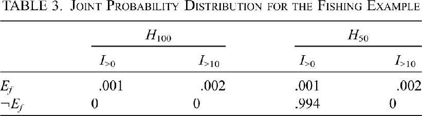
To illustrate the point, consider the joint distribution in table 3. I have added a proposition, I _>0, which is the claim that the net used had very tiny holes capable of catching the smallest fish. With this additional possibility added, the probabilities given are compatible with all of the facts above. In particular, P(E_f|H ₁₀₀) = 1 ≫ P(E_f|H ₅₀) = .003, and P(E_f|H ₁₀₀, I _>10) = P(E_f|H ₅₀, I _>10) = 1.

Table 3.Joint Probability Distribution for the Fishing Example

	H 100	H 50
	I >0	I >10	I >0	I >10
Ef	.001	.002	.001	.002
¬Ef	0	0	.994	0

However, we can see that learning I _>10 at the outset strongly favored the hypothesis H ₁₀₀ since P(I _>10|H ₁₀₀) = 0.67 ≫ P(I _>10|H ₅₀) = 0.002. Likewise, according to ALL iv, the aggregate information overwhelmingly favors H ₁₀₀ over H ₅₀ to a degree given by . This conclusion is not surprising given the details of the example. The distribution given in table 3 is plausible in that those who frequently fish a particular lake are more likely to use nets with large holes if the lake contains mostly large fish—they may not know the distribution of fish in the lake, but they know what works. Whatever story one might tell to account for the particular probabilities in this case, the upshot is that if an OSE renders a particular observation irrelevant in a particular context it is still possible for the aggregate information to discriminate between hypotheses.

While Eddington’s fishing example illustrates the way in which previously acquired information can deprive subsequent evidence of relevance, there is another example in the literature more closely analogous to the fine-tuning case.Footnote ¹⁴ This scenario involves firing squads. We are asked to imagine that a firing squad staffed by 12 expert marksmen takes aim at the prisoner to be executed. Each marksman fires 12 times when given the signal. When the smoke clears, we discover that the prisoner is still unharmed. Call the fact of this surprising survival E_s. In this case, we are interested in what the prisoner can infer from E_s concerning the following two hypotheses:

At first we might think that the prisoner has ample reason to favor H _con over H _miss since, given that these are expert marksmen, P(E_s|H _con) ≫ P(E_s|H _miss). However, in making his analysis the prisoner left out some pertinent information about the manner in which the observation of E_s was made:

According to those who would single out background information, we must incorporate I_O into the likelihoods by conditioning. In this view, the prisoner suffers from an OSE and cannot distinguish between the two hypotheses at all since P(E_s|H _con, I_O) = P(E_s|H _miss, I_O) = 1. Because I_O entails E_s, so the argument goes, learning E_s can tell the prisoner nothing about which hypothesis to favor. Thus, the prisoner in the grip of a strong OSE cannot reasonably conclude there was a conspiracy to save his life.

At this point, the tight analogy with the FTA should be clear. The prisoner stands in for us carbon-based life-forms. While the prisoner is attempting to assess whether design or chance is responsible for his survival, in the FTA we are attempting to infer design in the cosmos. In both cases, it has been objected that the observer suffers from an OSE that prevents discrimination between hypotheses. Supporters of the FTA invoke the firing-squad scenario because they think that our intuition strongly opposes the OSE objection—surely the prisoner can reasonably conclude that conspiracy is the better hypothesis. By analogy, they claim that we can conclude that an OSE is not a problem for the FTA.

In both cases, ALL tells us that the role of the OSE has been misinterpreted. It is true that, in the context of knowing that it was himself who made the observation, the prisoner learns nothing further by noting that he is alive. Likewise, it is the case that, knowing that all physics is done by carbon-based life-forms, we learn nothing further by discovering that the constants of physical law are just right to sustain carbon-based life. Nonetheless, the aggregate information might still favor one hypothesis over the other. In the firing-squad scenario, it is eminently plausible that P(E_s, I_O|H _con) ≫ P(E_s, I_O|H _miss). In the case of fine-tuning, it may be that P(E, I|H_D) > P(E, I|H_C). This will be the case if P(I|H_D) > P(I|H_C). I certainly do not wish to argue that this is in fact the case—there seem to be insurmountable difficulties in providing a well-defined measure corresponding to P(I|H_D).Footnote ¹⁵ My point is just that, when one distinguishes between contextual and total support, the presence of an OSE does not prove fatal to design arguments in either the firing-squad or the FTA case.

8. Conclusion

Insofar as one is inclined to accept LL as a framework for inference, no modification is necessary in order to deal with background information—unpacking LL leads to ALL. The interpretive key is the discrimination of two questions, one concerning the immediate support provided by a piece of evidence in context and one concerning the overall support provided by the total set of evidence. Looked at in this way, it becomes clear that objections based on observer bias are not necessarily fatal to the FTA. It is true that we, as carbon-based life-forms, cannot use the fact that some physical constants are just right for the existence of carbon-based life to discriminate between design hypotheses and their rivals. However, it may be the case that the aggregate evidence (including the fact of our existence) might permit such discrimination. Whether this is the case must be settled on other grounds.