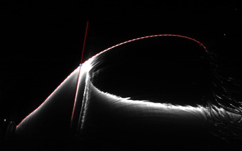
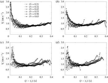
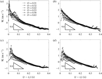
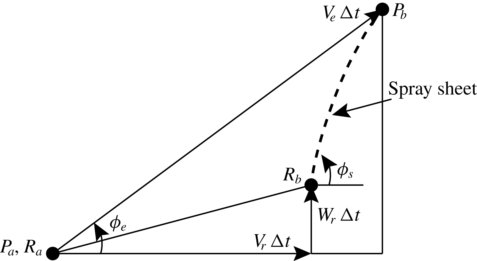
1 Introduction
During the planing motion of a high-speed planing craft or the landing of an amphibious aircraft, the hull frequently impacts with water waves. Knowledge about the formation of the water spray during the impact process is crucial for understanding this complex physical process. The spray formation covers a wide range of spatial and temporal scales and includes many physical processes, such as water sheet formation, wave propagation, air entrainment and the generation of droplets.
Theoretical investigations on general water impact phenomena include early work such as Wagner (Reference Wagner1932) and more recent studies such as Howison, Ockendon & Wilson (Reference Howison, Ockendon and Wilson1991), Korobkin (Reference Korobkin1994), Scolan & Korobkin (Reference Scolan and Korobkin2001), Korobkin & Scolan (Reference Korobkin and Scolan2006) and Oliver (Reference Oliver2007). Water impact problems in the context of naval science have been studied extensively, see for example Chuang & Milne (Reference Chuang and Milne1971), Chuang (Reference Chuang1973), Greenhow & Lin (Reference Greenhow and Lin1983), Vorus (Reference Vorus1996), Ulstein & Faltinsen (Reference Ulstein and Faltinsen1996) and Faltinsen, Kvålsvold & Aarsnes (Reference Faltinsen, Kvålsvold and Aarsnes1997). A considerable number of fundamental studies on the subject of water entry have been conducted focusing primarily on the impact of simple structures, such as cylinders (Kiara, Paredes & Yue Reference Kiara, Paredes and Yue2017), flat plates of various shapes (Iafrati & Korobkin Reference Iafrati and Korobkin2004, Reference Iafrati and Korobkin2008; Faltinsen & Semenov Reference Faltinsen and Semenov2008; Huera-Huarte, Jeon & Gharib Reference Huera-Huarte, Jeon and Gharib2011; Peters, van der Meer & Gordillo Reference Peters, van der Meer and Gordillo2013; Wang et al. Reference Wang, Wang, Balaras, Conroy, O’Shea and Duncan2016, Reference Wang, Kim, Wong, Yu, Kiger and Duncan2019; Mayer & Krechetnikov Reference Mayer and Krechetnikov2018), wedges (Dobrovol’Skaya Reference Dobrovol’Skaya1969; Zhao & Faltinsen Reference Zhao and Faltinsen1993; Semenov & Iafrati Reference Semenov and Iafrati2006; Vincent et al. Reference Vincent, Xiao, Yohann, Jung and Kanso2018), cones (Marston & Thoroddsen Reference Marston and Thoroddsen2014), spheres (Thoroddsen et al. Reference Thoroddsen, Etoh, Takehara and Takano2004; Duez et al. Reference Duez, Ybert, Clanet and Bocquet2007; Truscott & Techet Reference Truscott and Techet2009; Marston et al. Reference Marston, Truscott, Speirs, Mansoor and Thoroddsen2016) and paraboloids (Wu & Sun Reference Wu and Sun2014). The behaviour of the spray generated during the impact varies significantly with the impactor’s geometry. The remainder of this review will focus on the spray formation during the impact of structures that create splash phenomena relevant to the present study.
The evolution of the water surface underneath an impactor during its water entry has been studied extensively. Typically, in cases where the impactor has moderate vertical impact speed and sharpness near its nose, as the leading edge of the impactor enters the water surface, the adjacent water surface rises and turns over to form a water layer that is attached to the surface of the impactor. A number of theoretical studies investigated the very early stage of the impact or the impact with very large impact speed. As a result, gravity has often been ignored in these work. Dobrovol’Skaya (Reference Dobrovol’Skaya1969) derived an implicit similarity form of the water surface profile under a symmetric infinitely long wedge as it enters the water surface. The theory assumes a constant vertical velocity of the wedge and a linear temporal dependence for the length scale of the flow system. The numerical calculation of this similarity solution was performed down to a deadrise angle of
 $30^{\circ }$
. The similarity solution of Dobrovol’Skaya (Reference Dobrovol’Skaya1969) was numerically obtained at smaller deadrise angles by Zhao & Faltinsen (Reference Zhao and Faltinsen1993) and Wang & Faltinsen (Reference Wang and Faltinsen2017). In de Divitiis & de Socio (Reference de Divitiis and de Socio2002), the flow field under the body is calculated in similarity form during the impact of a wedge on a free surface by first imposing a series of potential flow singularities with unknown intensities and then determining these intensities through boundary conditions and an optimization technique. Semenov & Iafrati (Reference Semenov and Iafrati2006) studied the effect of asymmetry during the water entry of a tilted wedge by using potential flow formulations and computed the self-similar free-surface evolution. The calculation shows that there is a cross-flow near the apex of a tilted wedge and this flow is responsible for the variation in water surface evolution and pressure distribution compared to the symmetric water entry of a vertically oriented wedge. Using analytical and numerical calculations, Faltinsen & Semenov (Reference Faltinsen and Semenov2008) studied the water surface evolution under a semi-infinitely long flat plate with various vertical or oblique velocities when it enters the water surface at different deadrise angles. In the vertical impact calculations in Zhao & Faltinsen (Reference Zhao and Faltinsen1993) and Faltinsen & Semenov (Reference Faltinsen and Semenov2008), the under-plate jet tip intersects with the plate’s surface at an non-zero angle and this angle decreases and asymptotically approaches zero as the plate’s deadrise angle decreases to zero. Of course, viscous effects within the boundary layer along the impactor’s surface are not accounted for in these potential flow calculations. Also, phenomena involving topological changes of the air–water interface, such as the formation of droplets and ligaments, which are likely to occur for cases with large impact speeds and small deadrise angles, are not considered. Nevertheless, the potential flow theory should be able to favourably describe the bulk flow field outside the boundary layer. Marston & Thoroddsen (Reference Marston and Thoroddsen2014) performed an experimental study of the splash layer adjacent to the surface of a series of cones as they enter the free surface of various liquids. It was found that a thin layer of air is formed between the spray and the cone surface when the liquid has high viscosity or low surface tension or when the cone surface is hydrophobic. It was also found that the collapse of spray profiles in similarity form fails as the influence of viscosity becomes prominent, i.e. with low impact speeds or with high-viscosity liquids. Iafrati (Reference Iafrati2016) reported an experimental study of the oblique impact of a large-scale flat plate on a water surface at high horizontal velocities. The spray generated under the plate was found to break up into droplets quickly after it emerges from the spray root, which propagates at high speed along the plate. Relevant to Iafrati (Reference Iafrati2016), a computational study of the high-speed oblique impact of a two-dimensional elastic plate with both ends free is reported in Reinhard, Korobkin & Cooker (Reference Reinhard, Korobkin and Cooker2013).
In cases where the impactor has a finite width, a violent surface motion is generated outboard of the edge of the impactor and this surface motion is strongly affect by the impactor geometry and motion profile. Iafrati & Korobkin (Reference Iafrati and Korobkin2004) performed a numerical study of the water surface evolution outboard of a horizontally orientated flat plate during the initial period of the impact. The results indicate that the flow near the plate edge is self-similar and that the thickness of the outboard jet decreases as the distance from the plate increases. The similarity solution of the water entry of a wedge or plate with expanding width is reported in Semenov & Wu (Reference Semenov and Wu2016). The calculation was performed with various expansion rates and the behaviour of the splash jet after the flow detaches from the solid surface is explored. Peters et al. (Reference Peters, van der Meer and Gordillo2013) performed an experimental study of the outboard splash generated during the impact of a horizontally orientated round disk on a water surface. The splash profiles outboard of the disk were found to be self-similar and the temporal dependence of the profiles follows a
 $t^{2/3}$
power law. The
 $t^{2/3}$
power law of the evolution of water surface is also found in the numerical calculations of the water entry of a circular disk (Iafrati & Korobkin Reference Iafrati and Korobkin2011) and a flat plate (Iafrati & Korobkin Reference Iafrati and Korobkin2008). In Peters et al. (Reference Peters, van der Meer and Gordillo2013), it was found that droplets break up from the tip of the splash due to Rayleigh–Taylor instability and that their size is nearly independent of the impact Weber number. In the experimental study by Marston et al. (Reference Marston, Truscott, Speirs, Mansoor and Thoroddsen2016), the splash generated during the vertical impact of spheres on the surface of several liquids under various ambient pressures was investigated. An initially nearly vertical crown splash was observed next to the sphere. A buckling instability phenomenon, which is characterized by striations near the tip of the splash before the closure of the crown splash, is also reported. It was found that the number of striations and the spacing between striations both increase with the size of the sphere. In a recent study by Vincent et al. (Reference Vincent, Xiao, Yohann, Jung and Kanso2018), the splash generated during the vertical water entry of small wedges of various deadrise angles was studied. It is pointed out that there exists a low-pressure area under the splash sheet due to air flow and that this flow is partially responsible for the shape of the splash. An experimental study on the impact of a horizontally oriented flat rectangular plate on liquid surfaces is reported in Mayer & Krechetnikov (Reference Mayer and Krechetnikov2018). This work discussed characteristics of the flow field, water surface motion and the air layer entrapped in areas close to the edge of the plate during the early stage of the impact. It is reported that the surface profiles of the ejecta are nearly self-similar and that the self-similarity exponent varies with impact conditions. The departure angle of the ejecta at the horizontal plate’s edge was found to be non-zero under some conditions.
One of the difficulties in analysing gravity-driven impact problems is that the hydrodynamic load on the impactor is highly transient and nonlinear and is an unknown quantity that is in turn coupled with the motion of the impactor. This problem is particularly important when the deadrise angle of the impactor is small, owing to the sudden change of significant hydrodynamic load. The coupled motion of the impactor and the flow is not the focus of the present paper but is discussed in several studies of gravity-driven impact, such as Wang, Lugni & Faltinsen (Reference Wang, Lugni and Faltinsen2015a ,Reference Wang, Lugni and Faltinsen b ) and Bao, Wu & Xu (Reference Bao, Wu and Xu2017). When the impactor is given a prescribed motion, as it is in many theoretical studies and in the present experimental study, this coupling is eliminated.
In the present paper, the impact of a flat plate on a quiescent water surface is studied experimentally. The plate is held in an orientation tilted up from horizontal about one of its long edges, which is positioned close to a vertical wall. The plate, is driven by a computer-based feedback control motion system before and during the impact. The motion profiles of the plate are programmed and accurately controlled, allowing the impact process to be independent of hydrodynamic loads on the plate or the weight of the moving structure. This novel system allows for the study of the spray formation within a highly controllable parameter space. In particular, the dimensionless motion profiles,
 $Z/B$
versus
 $W/W_{0}$
(where
 $Z$
is the instantaneous plate height,
 $B$
is the plate width,
 $W$
is the instantaneous plate speed and
 $W_{0}$
is the plate impact speed) for all experimental conditions fall on a single curve. The evolution of the water surface profiles are measured with high temporal and spatial resolution. These parametric motion profiles and the highly resolved measurements allow for the examination of the spray’s behaviour in several aspects that have not been explored in the past. The large size and the relatively small deadrise angle of the plate were chosen to be similar to practical problems such as slamming between a planing boat or amphibious aircraft and a water wave. However, it should be noted that in the present experiments, the no-slip boundary condition on the vertical wall and the flow through the 2 mm gap between the plate’s leading edge and the wall probably produce effects that make the flow in some ways dissimilar to the flow on one side of a wedge during impact. Further discussion of these effects are given in the paper.
In flat plate impact studies, several of the important dimensionless parameters are the tilt of the plate relative to horizontal (
 $\unicode[STIX]{x1D6FD}$
, the deadrise angle), the Froude number (
 $\mathit{Fr}=W_{0}/\sqrt{gB}$
, where
 $W_{0}$
is the vertical impact velocity,
 $B$
is the width of the plate and
 $g$
is the gravitational acceleration), the Reynolds number (
 $\mathit{Re}=W_{0}B/\unicode[STIX]{x1D708}$
, where
 $\unicode[STIX]{x1D708}$
is the kinematic viscosity of water) and the Weber number (
 $\mathit{We}=\unicode[STIX]{x1D70C}W_{0}^{2}B/\unicode[STIX]{x1D70E}$
, where
 $\unicode[STIX]{x1D70C}$
is the density of water and
 $\unicode[STIX]{x1D70E}$
is the surface tension of water). In the present experiments,
 $10^{\circ }\leqslant \unicode[STIX]{x1D6FD}\leqslant 25^{\circ }$
,
 $0.21\leqslant \mathit{Fr}\leqslant 0.63$
,
 $1.5\times 10^{5}\leqslant \mathit{Re}\leqslant 4.6\times 10^{5}$
and
 $862\leqslant \mathit{We}\leqslant 7758$
. These values show similarity to the hull deadrise angles of high-speed boats and the dominance of inertia and gravity in the flow dynamics. These experiments also compliment the recent wedge impact experiments of Vincent et al. (Reference Vincent, Xiao, Yohann, Jung and Kanso2018), which was performed with
 $30^{\circ }\leqslant \unicode[STIX]{x1D6FD}\leqslant 60^{\circ }$
and with
 $2.0\leqslant \mathit{Fr}\leqslant 6.0$
, at high
 $\mathit{Re}$
and
 $\mathit{We}$
.
The remainder of this paper is organized in the following order. The details of the experimental set-up are presented in § 2, the results and discussion of the spray formation during the impact will be given in § 3 and conclusions are drawn in § 4.
2 Experimental details
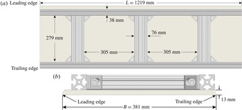
The experimental facility and laser-induced fluorescence (LIF) set-up for the outboard spray measurements are shown in side view (a) and end view (b). The end view of the LIF set-up for the under-plate spray measurements is shown in (c). In (a), only one of the plate’s long edges, the one closest to the viewer, is shown.

Schematic drawings of the impact plate structure, which consists of a 12.7 mm thick polycarbonate plate that is glued using marine grade epoxy to an aluminium frame. In the aluminium frame, the two long side pieces are 1515 T-slot profile beams and the three short pieces are profile 1530 T-slot profile beams, both manufactured by
 $80/20$
, Inc.

2.1 Facilities
The experiments were performed in a towing tank that is 13.7 m long, 2.4 m wide and 1.3 m tall, see figure 1. The four sides and bottom of the tank consist of a set of 3.5 cm thick clear Acrylic flat panels that are in turn supported by an external steel superstructure that is bolted to the laboratory floor. A water surface skimmer is installed along one of the 2.4 m long tank walls and is connected to a pump and diatomaceous earth filter. The water that enters the skimmer is either sent to the drain or filtered and pumped back to the tank at the opposite end from the skimmer.
The tank includes a two-axis carriage system with horizontal and vertical motion, though only vertical motion was used in the present study. The carriage consists of two stainless steel sheet metal boxes, called herein the vertical and horizontal carriages, that are constructed with internal bulkheads and beams in manner that creates very stiff and relatively light structures. The box that forms the horizontal carriage is rectangular and rides on two parallel precision horizontally oriented rails that are mounted, one above the other, on a 2.97 m tall steel frame that was constructed next to one of the long side walls of the tank. The frame is mounted to the 0.8 m thick concrete floor and 0.3 m thick side wall of the laboratory. With this mounting, the possibility of structural vibrations caused by the carriage motion reaching the tank and generating unwanted water waves is extremely low. The box that forms the vertical carriage is trapezoidal in cross-section and rides on two vertically oriented rails that are mounted on the horizontal carriage. The vertical carriage is driven by a belt and electric servo motor system and is controlled by a single computer program that uses position feedback to execute programmable motions. As can be seen in figure 1, the model that is support by the carriage moves near one of the long side walls of the tank and thereby allows for a wide cross-tank area for development and measurement of the water surface motion created by the model impact.
The model used in the present experiments is a polycarbonate plate (length
 $L=121.9~\text{cm}$
, width
 $B=38.1~\text{cm}$
, thickness
 $\unicode[STIX]{x1D70F}=1.3~\text{cm}$
, and elastic modulus 2.6 GPa) whose upper surface is glued using marine epoxy to a frame of aluminium beams as shown in figure 2. In addition to the overall attachment via the epoxy, a bolt was placed in each corner of the plate to connect it to the frame as a safety precaution in case the epoxy were to separate from the plate or the beams during impact with the water surface. The bolt heads were counter sunk into the plate and the remaining indentation in the plate surface was filled with silicon sealant and smoothed to be flush with the otherwise pristine under surface of the plate. The aluminium beams are made of 6105-T5 alloy, which has a modulus of elasticity of 70 GPa. The second moment of area of the beam cross-sections are
 $1.06\times 10^{-7}~\text{m}^{4}$
and
 $2.01\times 10^{-7}~\text{m}^{4}$
for the longitudinal and transverse components, respectively. The quasi-static deflection of the plate due to the bending of the aluminium frame and of the polycarbonate plate in the two 305 mm by 279 mm openings in the aluminium frame, see figure 2, were estimated using one-dimensional Euler beam theory and two-dimensional finite element analysis, respectively. In the deflection estimation, the asymptotic pressure distribution on the surface of a rigid wedge at various times during vertical water entry (see Zhao & Faltinsen Reference Zhao and Faltinsen1993) was used and the coupling between the hydrodynamic load and the structural deformation was not considered. At the smallest deadrise angle
 $\unicode[STIX]{x1D6FD}=10^{\circ }$
and largest impact speed
 $W_{0}=1.2~\text{m}~\text{s}^{-1}$
in the present experiments, the largest estimated deflection of the plate section in the frame openings, of the longitudinal beams and of the mid transverse beam, where the main measurement plane is located, is 0.34 mm, 0.17 mm and
 $1.68~\unicode[STIX]{x03BC}\text{m}$
, respectively. Thus, the deformation of the combined plate structure is very small and its influence on the spray generation is considered negligible.
The stiffened plate is attached to the vertical carriage via a system of aluminium beams and is set so that its long edges are horizontal and its short edges are tilted with a deadrise angle,
 $\unicode[STIX]{x1D6FD}$
, relative to the plane of the water surface. When set up in this way, the lower (upper) long edge of the plate is called the leading (trailing) edge.
A vertical wall (called herein the symmetry wall) is installed close to the leading edge of the impact plate, see figure 1. The wall consists of a set of polycarbonate plates, on the side closest to the impact plate, see figures 1(a) and 1(b), that are bolted to and stiffened by a framework of aluminium beams that are in turn attached to the tank’s steel superstructure. The leading edge of the impact plate model moves vertically along this wall. As can be seen in figure 2(b), the upper corner of the impact plate’s leading edge was trimmed off so that the small gap between the edge of the plates’ impact surface and the smooth surface of the symmetry wall can be held nearly constant for all
 $\unicode[STIX]{x1D6FD}$
. The width of the gap was adjusted to minimize its effect on the experimental results, see discussion in § 2.4.
2.2 Surface profile measurements
The water surface profile histories generated during the impact are measured with a cinematic laser induced fluorescence technique (Liu & Duncan Reference Liu and Duncan2006; Wang et al. Reference Wang, Wang, Balaras, Conroy, O’Shea and Duncan2016, Reference Wang, Ikeda-Gilbert, Duncan, Lathrop, Cooker and Fullerton2018, Reference Wang, Kim, Wong, Yu, Kiger and Duncan2019). The laser light sheet used in these measurements is created from a 6 Watt argon ion laser and a system of spherical and cylindrical lenses. The light sheet is approximately 1 mm thick as it enters the still water surface. The water in the towing tank is mixed with fluorescein dye at a concentration of approximately 5 ppm. A high-speed digital movie camera (Phantom V642, Vision Research, Inc., 4-megapixel images, 12-bit grey levels) is used to record images of the intersection of the laser light sheet with the water free surface and a long-wavelength-pass optical filter placed in front of the camera lens blocks out the specular reflections of laser light while allowing the light from the fluorescing dye to reach the image sensor. The digital images are processed using gradient-based techniques to determine the profile of the water surface in each image.
The cinematic LIF system is used in separate configurations to measure the water surface profile evolution in the regions underneath and outboard of the plate. The camera and light-sheet set-up for the outboard measurements is shown in figures 1(a) and1(b) and the light-sheet set-up for the under plate measurements is shown in figure 1(c). For the outboard profile measurements, two high-speed cameras are installed above the tank and view the outboard water surface region as shown in figure 1(b). In order to have a large field of view and because of the large angle between the camera optical axis and the normal to the plane of the light sheet, the main profile camera (Camera I) is fitted with a 45 mm tilt-shift lens. This camera is operated at a frame rate of 800 Hz and has a spatial resolution of
 $0.5~\text{mm}~\text{pixel}^{-1}$
with image dimensions of
 $1600\times 2560$
pixels. A second camera (II), positioned next to Camera I, is fitted with a 60 mm lens and views a smaller region of the free surface next to the trailing edge of the plate. This camera, which is used for detailed examination of the Type I spray (see § 3.2.1 for definition), is set at a higher frame rate (2400 Hz) and has a spatial resolution of
 $0.4~\text{mm}~\text{pixel}^{-1}$
with image dimensions of
 $900\times 2560$
pixels. In the under-plate profile measurements, the laser beam is directed horizontally across the width of the tank toward the leading edge of the plate. The light sheet illuminates the bottom surface of the impact plate and the water surface below. A third camera (III) is installed at one end of the tank, views a
 $19\times 31~\text{cm}$
measurement window at a frame rate of 800 Hz and has a spatial resolution of
 $0.3~\text{mm}~\text{pixel}^{-1}$
. For both profile measurement configurations, the distortions created by the lenses and the large view angles are corrected by using images of a checkerboard calibration target that was placed in the plane of the light sheet. The corner points on the calibration target are first extracted from the images and a third-order polynomial is used for the transformation of coordinates from the image reference frame to the calibration target reference frame. An LIF image of the still water surface is taken before each experimental run and the extracted still water level line is defined as the
 $y$
-axis. The details of this calibration process can be found in Wang et al. (Reference Wang, Ikeda-Gilbert, Duncan, Lathrop, Cooker and Fullerton2018).
2.3 Plate motion profiles and experimental conditions
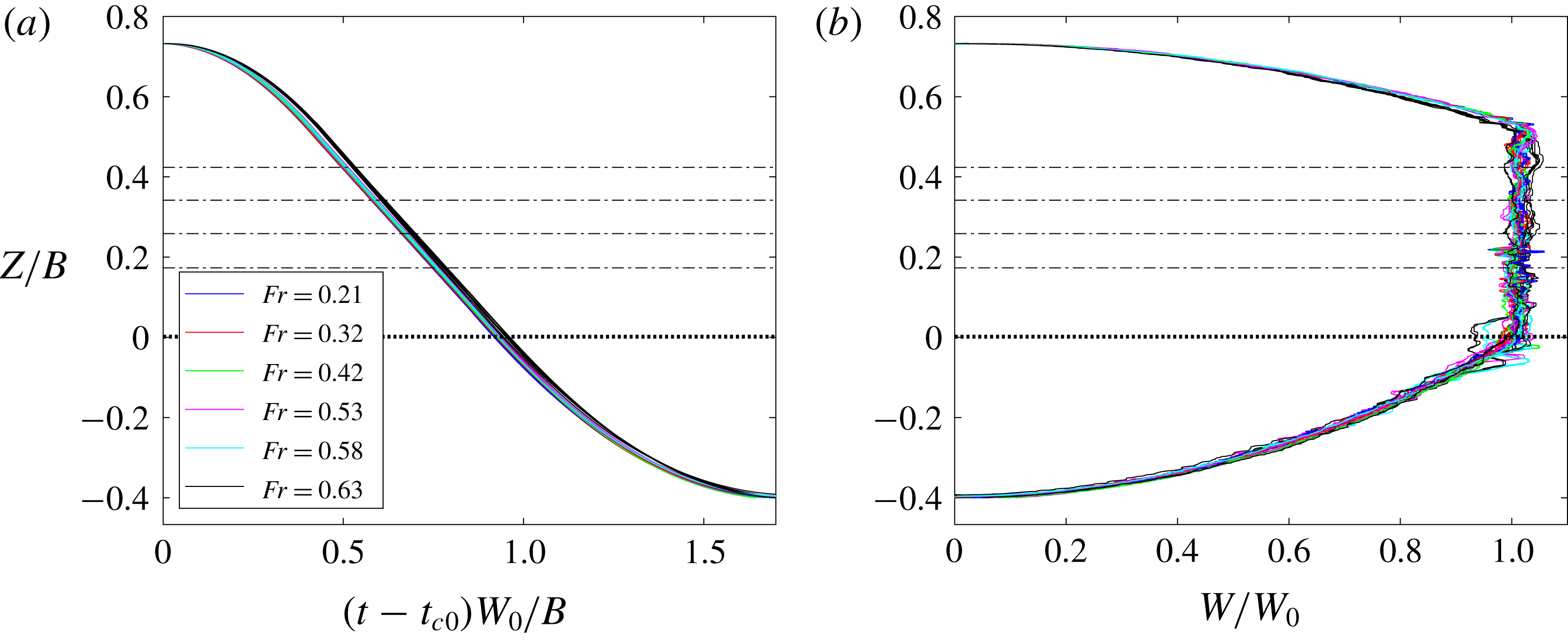
Carriage motion profiles on plots of dimensionless vertical position of the plate’s leading edge (
 $Z/B$
) versus dimensionless time
 $(t-t_{c0})W_{0}/B$
(a) and dimensionless carriage speed
 $W/W_{0}$
(b), where
 $t_{c0}$
is the time when the vertical carriage motion begins. Two repeated runs are plotted for each of the 24 experimental conditions. For each value of
 $\unicode[STIX]{x1D6FD}$
, the water level is adjusted so that the plate’s trailing edge reaches the still water level when the leading edge reaches
 $Z/B=0$
. The four still water levels,
 $Z/B=\sin \unicode[STIX]{x1D6FD}$
, are marked by the four horizontal dash-dot lines.

In each run, the carriage starts at a position well above the water surface, accelerates to a constant speed (
 $W_{0}$
) while still in the air, maintains that speed until the plate’s trailing edge reaches the still water level and then decelerates to a stop. The distances over which the carriage accelerates, remains at constant speed and decelerates are held constant at
 $Z_{1}=0.2B$
,
 $Z_{2}=0.53B$
and
 $Z_{3}=0.4B$
, respectively, for all experimental conditions. The programmed dimensionless carriage vertical position
 $Z/B$
versus
 $t^{\prime }$
is given by
 $$\begin{eqnarray}\frac{Z(t)}{B}=\left\{\begin{array}{@{}ll@{}}\displaystyle \frac{B}{4Z_{1}}t^{\prime 2} & \displaystyle \text{for}\quad 0\leqslant t^{\prime }\leqslant \frac{2Z_{1}}{B},\\ \displaystyle t^{\prime }-\frac{Z_{1}}{B} & \displaystyle \text{for}\quad \frac{2Z_{1}}{B}<t^{\prime }\leqslant \frac{2Z_{1}+Z_{2}}{B},\\ \displaystyle -\frac{B}{4Z_{3}}t^{\prime 2}+\left(1+\frac{2Z_{1}+Z_{2}}{2Z_{3}}\right)t^{\prime } & \\ \displaystyle -\frac{(2Z_{1}+Z_{2})^{2}}{4Z_{3}B}-\frac{Z_{1}}{B} & \displaystyle \text{for}\quad \frac{2Z_{1}+Z_{2}}{B}<t^{\prime }\leqslant \frac{2Z_{1}+Z_{2}+2Z_{3}}{B},\end{array}\right.\end{eqnarray}$$
where
 $t^{\prime }=(t-t_{c0})W_{0}/B$
is the dimensionless time and
 $t^{\prime }=0$
is at the instant when the carriage motion begins. A plot of the measured
 $Z/B$
, versus
 $t^{\prime }$
for all 24 experimental conditions is given in figure 3(a) where it can be seen that the data collapse well to a single curve. A plot of
 $Z/B$
versus the measured dimensionless carriage speed,
 $W/W_{0}$
, for the 24 experimental conditions is shown in figure 3(b). These data also collapse well to a single curve except for a relatively modest level of noise which results primarily from the calculation of the instantaneous carriage velocity as the derivative with respect to time of the measured height,
 $Z$
. The largest deviation from the desired motion profile occurs near
 $Z/B=0$
for the
 $\unicode[STIX]{x1D6FD}=10^{\circ }$
cases with the highest speeds,
 $W_{0}=1.12$
and
 $1.22~\text{m}~\text{s}^{-1}$
. It is believed that the more rapid changes in force on the plate as the trailing edge hits the water in these cases is the cause of these larger deviations. See the figure caption for additional details.
A test matrix consisting of six impact speeds,
 $W_{0}=0.41$
, 0.61, 0.81, 1.02, 1.12 and
 $1.22~\text{m}~\text{s}^{-1}$
, and four deadrise angles,
 $\unicode[STIX]{x1D6FD}=10^{\circ }$
,
 $15^{\circ }$
,
 $20^{\circ }$
and
 $25^{\circ }$
, was chosen. The impact Froude number
 $\mathit{Fr}=W_{0}/\sqrt{gB}$
varies from 0.212 to 0.631; however, it should be kept in mind that this variation was created by varying only the plate speed,
 $W_{0}$
. As time proceeds during impact, the instantaneous Froude number, defined here as
 $\mathit{Fr}^{\prime }=W_{0}/\sqrt{g\ell (t)}$
, where
 $\ell$
is the instantaneous length from the leading edge of the plate to the intersection of the plate surface with the still water level, is initially high and decreases with time. The value of
 $\ell$
when
 $\mathit{Fr}^{\prime }=1.0$
varies from
 $0.044B$
for the lowest impact speed,
 $W_{0}=0.41~\text{m}~\text{s}^{-1}$
, to
 $0.397B$
for the highest,
 $W_{0}=1.12~\text{m}~\text{s}^{-1}$
. Thus, gravity plays a significant role in the flow dynamics during a substantial part of the impact process.
The sequence of steps performed for each experimental run takes approximately one hour. The sequence begins by raising the vertical carriage to the starting position where the plate is well above the water surface. Once in position, the plate is wiped with a soft cloth to remove any remaining water droplets. The water filtration system is then turned on for a period of approximately 15 min. After the filter is turned off, the water motion is allowed to die away over a period of about 40 min. An LIF image of the calm water surface is then taken with each camera, just before the next run takes place. By examination of these LIF images, the still water level is carefully monitored to ensure its consistency over runs at the same value of
 $\unicode[STIX]{x1D6FD}$
. Finally, the experimental run is initiated, after which the data from each camera and the position versus time record of the carriage motion are saved. The surface tension of the tank water was measured with a Wilhelmy plate device before the first run and after the last run of each day. The surface tension was maintained to that of clean water at room temperature,
 $73\pm 0.5~\text{dyn}~\text{cm}^{-1}$
.
2.4 The gap between the plate edge and the symmetry wall
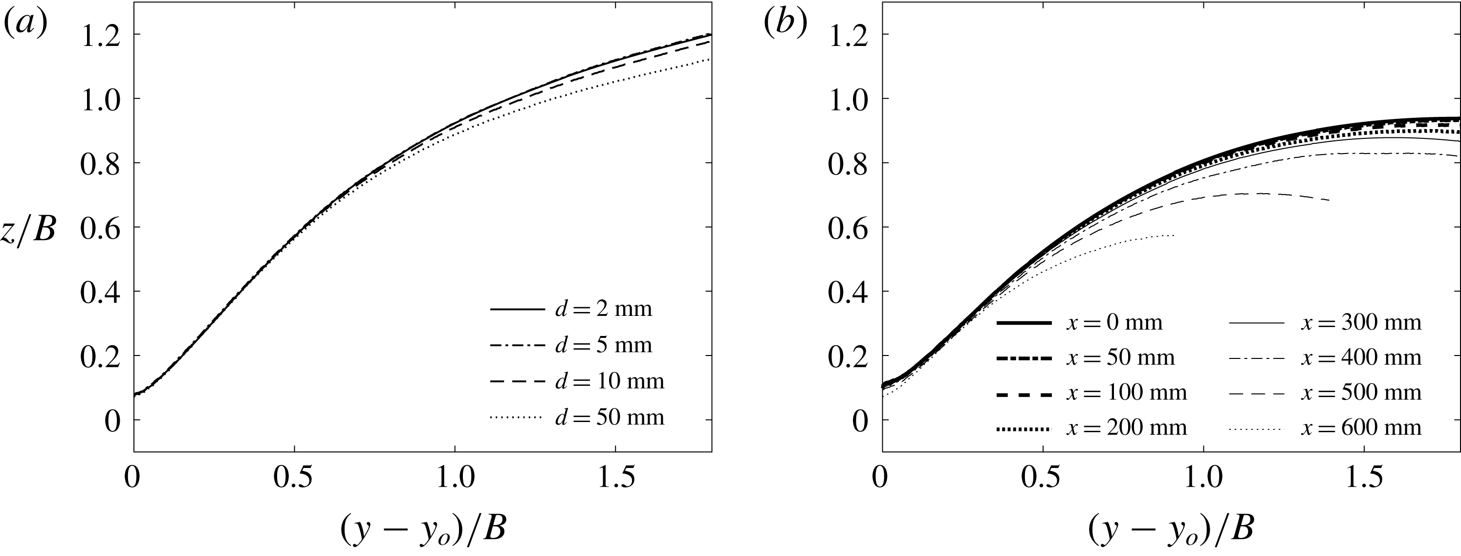
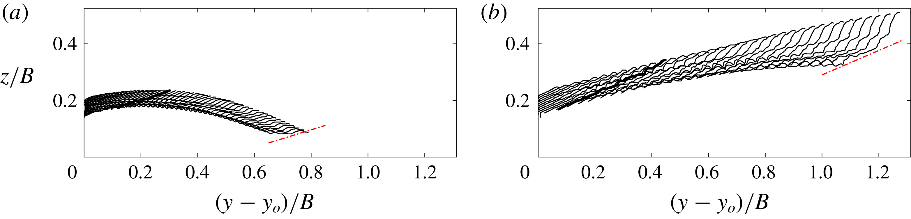
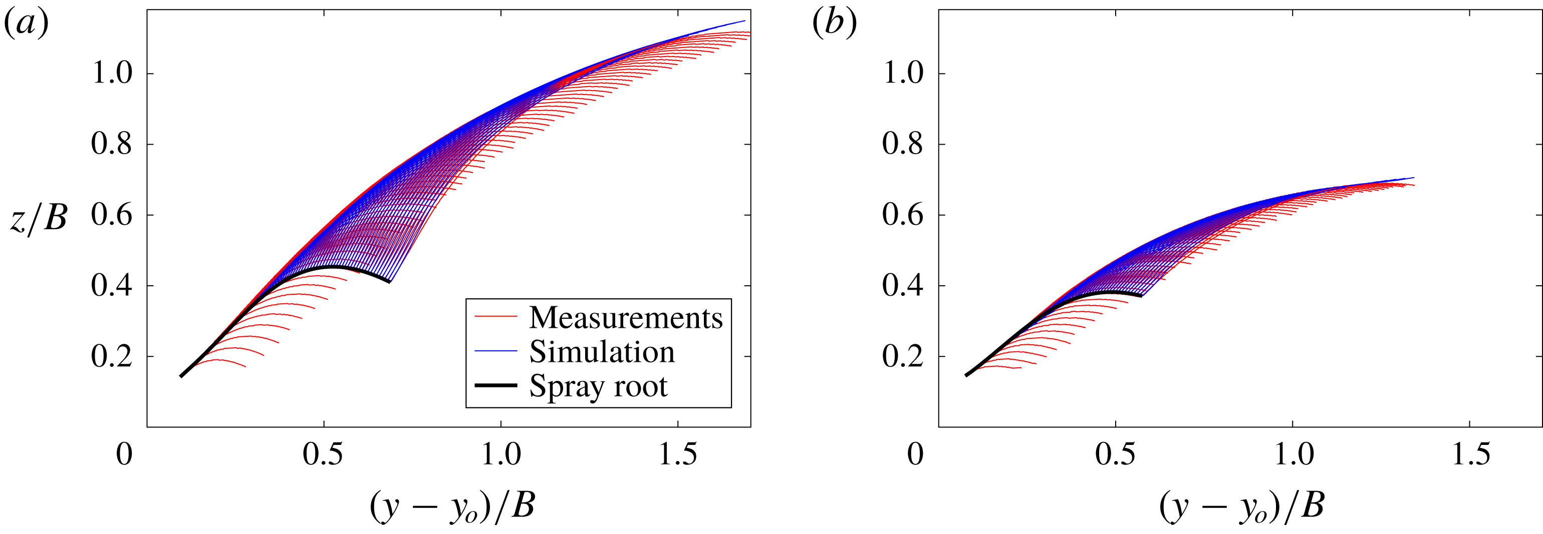
(a) Spray envelope for
 $\unicode[STIX]{x1D6FD}=15^{\circ }$
,
 $\mathit{Fr}=0.53$
and several gap widths (
 $d$
) between the leading edge of the plate and the symmetry wall. (b) Spray envelopes for
 $\unicode[STIX]{x1D6FD}=20^{\circ }$
,
 $\mathit{Fr}=0.53$
and a number of vertical planes located at positions (given by the coordinate
 $x$
) along the length of the plate. The mid-plane of the plate’s long edge is taken as
 $x=0$
. The still water level is at
 $z/B=0$
and the plate’s trailing edge is at
 $(y-y_{o})/B=0$
.

The width of the horizontal gap between the leading edge of the plate and the symmetry wall is expected to affect the behaviour of the spray. The ideal case would be zero gap width and therefore zero leakage of water through the gap. This case would be the most similar to the flow found in one side of a wedge during impact with free surface. It is thought that as the gap becomes larger the high pressure found at the leading edge would partially drive water through the gap rather than into the spray formation. To explore the effect of the gap width on the spray, a series of experiments with four gap widths (
 $d=2~\text{mm}$
, 5 mm, 10 mm, 50 mm),
 $\unicode[STIX]{x1D6FD}=15^{\circ }$
and
 $\mathit{Fr}=0.53$
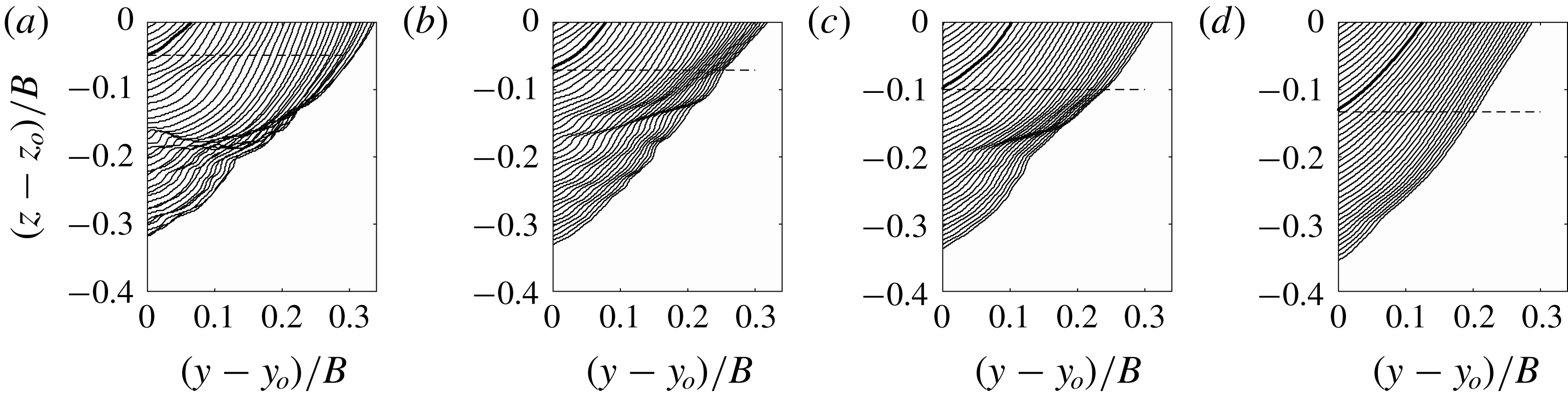
was performed. As the single spray feature to be compared for impacts with the four gap widths, the spray envelope was chosen. The spray envelope is the curve above which there is no spray and below which there is spray at all points at least at one instant during the impact process. This feature of the outboard spray is defined and discussed in detail in § 3.2.4, see figure 22. The spray envelopes for the four gap widths cases are shown in figure 4(a). As depicted in the plot, close to the trailing edge (at
 $y-y_{o}=0$
), the slopes of the envelopes are nearly the same for all four gap widths. Further away from the trailing edge, the height of the envelope at the same
 $y$
decreases as the gap width increases. This trend is more significant for
 $d=10~\text{mm}$
and
 $d=50~\text{mm}$
. As the gap width decreases, the variation between the envelopes decreases. Since the envelopes for
 $d=2~\text{mm}$
and
 $d=5~\text{mm}$
are nearly the same, further decrease in gap width is not expected to have a significant effect on the behaviour of the spray. In consideration of these findings, the gap width was set to 2 mm for the measurements presented in the remainder of this paper.
2.5 Effect of three-dimensionality
In order to explore the variation of the spray as a function of cross-stream position along the plate, a set of spray measurements were performed at seven cross-stream locations ranging from the centre plane (
 $x=0$
) to 1 cm away from the side edge of the impact plate (
 $x=600~\text{mm}$
). The spray envelope is used here to illustrate the effect of three-dimensionality on the spray. In this set of experiments,
 $\unicode[STIX]{x1D6FD}$
and
 $\mathit{Fr}$
were set to
 $20^{\circ }$
and 0.53, respectively, for all experimental runs. The resulting spray envelopes are shown in figure 4(b) where it can be seen that the height of the spray sheet decreases as the measurement plane moves away from the centre plane of the impact plate. At
 $x=600~\text{mm}$
(near the plate’s side edge), the maximum height of the spray envelope is approximately
 $2/3$
of that in the centre plane (
 $x=0~\text{mm}$
). In the range
 $x\in [0~\text{mm},100~\text{mm}]$
, the spray height does not vary significantly, indicating that the flow is nearly two-dimensional. In the spray measurements presented in the remainder of this paper, the light sheet is located at the centre plane (
 $x=0~\text{mm}$
) of the plate.
3 Results and discussion
The qualitative and quantitative descriptions of the spray generation process under the plate during the initial impact period and outboard of the plate after the trailing edge hits the local water surface are described separately in the following two subsections, § 3.1 and § 3.2, respectively.
3.1 Kinematics of the free-surface evolution under the plate
In this subsection, the evolution of the water surface profile under the plate is discussed. This part of the spray generation process starts when the leading edge of the plate hits the undisturbed water surface and extends to the time when the under-plate root (see the following subsection for definition) reaches the plate’s trailing edge. This flow is the precursor to the outboard spray described in § 3.2.
3.1.1 Qualitative description of the profiles
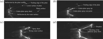
Sequence of images of the water surface profile under the plate. The images are from a high-speed LIF movie taken with
 $\mathit{Fr}=0.53$
and
 $\unicode[STIX]{x1D6FD}=25^{\circ }$
. The field of view of the images is
 $78~\text{cm}\times 31~\text{cm}$
. The movie was recorded at 800 pps and the time interval between the images shown here is 32.5 ms. The image in (a) was captured just after the plate’s leading edge hit the water surface and the image in (d) was captured as the under-plate spray root reached the plate’s trailing edge. The movie from which these images were taken is available as supplementary movie 1, at https://doi.org/10.1017/jfm.2019.630.

The behaviour of the spray under the plate is described qualitatively with the aid of figure 5, which contains four annotated LIF images taken from a movie of an impact at
 $\mathit{Fr}=0.53$
and
 $\unicode[STIX]{x1D6FD}=25^{\circ }$
. When the leading edge of the plate first touches the undisturbed water surface, defined as time
 $t=t_{0}=0$
, a jet, herein called the under-plate spray sheet, begins to form and move along the bottom surface of the plate toward its trailing edge, see figure 5(a). As the plate continues to move downward at constant speed, the water surface near the intersection of the still water level and the plate surface rises and connects to the spray sheet, which becomes a thin water layer that remains attached to the bottom surface of the plate under most experimental conditions, see figure 5(b–d). The under-plate spray root is defined as the flow region where the rising curved water surface connects the undisturbed tank water with the spray sheet. In the spray root, the point on the water surface with the smallest horizontal distance to the leading edge of the plate is herein called the under-plate root point, as illustrated in figure 5(b). The tangent to the water surface at the under-plate root point is vertical. Near the leading edge of the spray sheet, the water surface becomes increasingly irregular, possibly due to the combined effects of the initial impact, the air resistance and the friction at the surface of the plate. The friction from the plate is also possibly a function of surface properties of the plate. In the present experiments, the polycarbonate plate’s surface is not treated specifically for exploring the effect of hydrophobic or hydrophilic coatings. Later in the impact, some droplets break up from the tip of the sheet and fall into the water surface below, see images 5(c,d). After the tip of the spray sheet reaches the trailing edge of the plate, an increasing portion of the spray sheet becomes a free jet. While the under-plate portion of the spray sheet remains attached to the plate, the tip of the free jet portion of the sheet tilts upward. As the plate continues to move downward, the root moves horizontally and reaches the trailing edge. After the moment shown in figure 5(d), a complete surface profile can no longer be obtained from the LIF images, since the camera view of the water surface illuminated by the laser sheet is partially blocked by the curved portion of the airborne spray sheet between the light sheet and the camera. This feature can be observed in image (d), where it is labelled ‘bending of the airborne spray sheet’. In the following, the times when the leading edge of the spray sheet and the under-plate root point reach the trailing edge of the plate are defined as
 $t_{j}$
and
 $t_{r}$
, respectively (
 $t_{j}<t_{r}$
).
3.1.2 Quantitative description of the profiles
Profiles of the water surface under the plate for
 $\mathit{Fr}=0.53$
and two deadrise angles:
 $\unicode[STIX]{x1D6FD}=15^{\circ }$
(a,c,e) and
 $\unicode[STIX]{x1D6FD}=25^{\circ }$
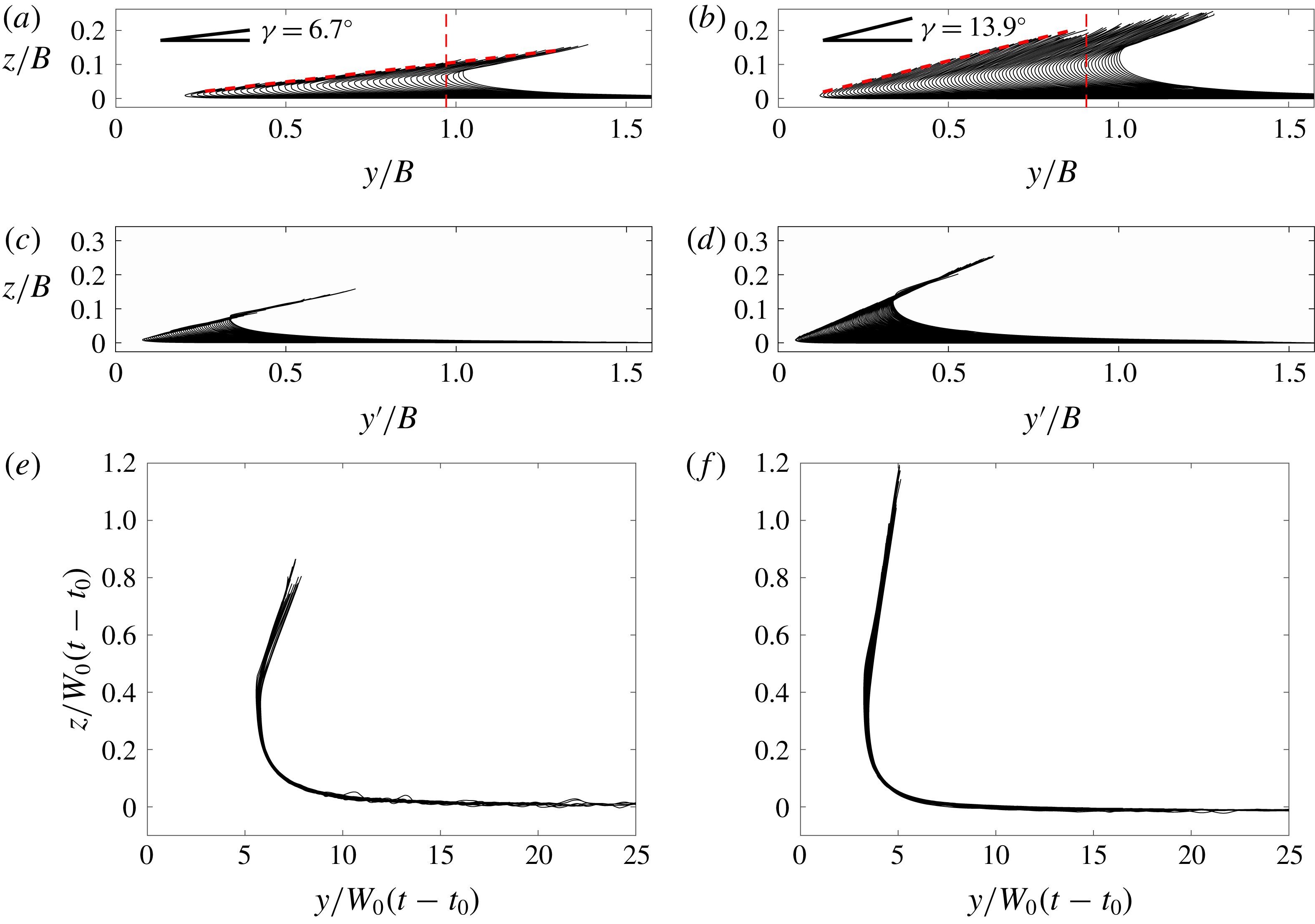
(b,d,f). The profiles in (a,b) are plotted in the laboratory reference frame, the profiles in (c,d) are plotted in a reference frame with the origin fixed at the geometrical intersection line (coordinates
 $y^{\prime }=y-W_{0}(t-t_{0})/\tan \unicode[STIX]{x1D6FD}$
,
 $z$
) and the profiles in (e,f) are scaled by
 $W_{0}(t-t_{0})$
and plotted in the laboratory reference frame. The
 $z$
axis points vertically up with
 $z=0$
at the still water level and the
 $y$
axis is horizontal with
 $y=0$
at the horizontal position of the plate’s leading edge. The vertical dashed lines in (a,b) indicate the trajectories of the plate’s trailing edge.

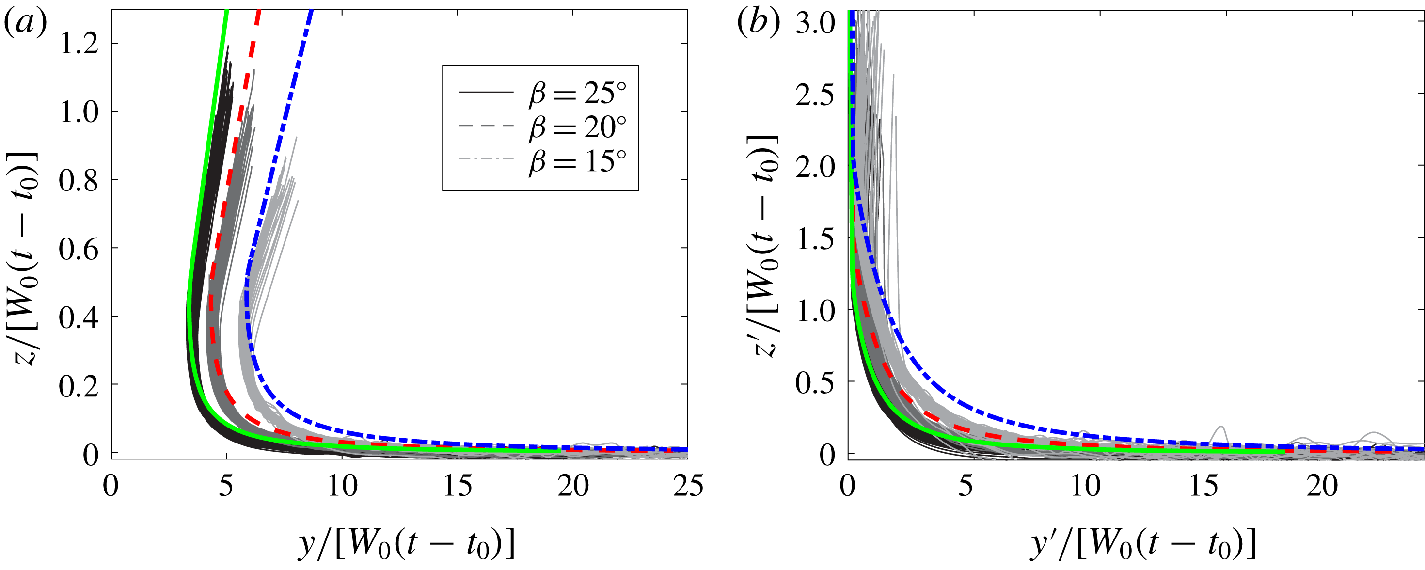
Plots of the underplate free-surface profiles scaled by
 $W_{0}(t-t_{0})$
for all deadrise angles
 $\unicode[STIX]{x1D6FD}$
and Froude numbers
 $\mathit{Fr}$
. In (a), the profiles are plotted in a laboratory-fixed reference frame. In (b), the
 $y^{\prime }$
–
 $z^{\prime }$
coordinate system moves horizontally with the geometrical intersection point,
 $(y^{\prime },z^{\prime })=(0,0)$
. The
 $y^{\prime }$
axis is at the still water surface and the
 $z^{\prime }$
axis is along the bottom surface of the plate. The thick coloured lines are the similarity solution given theoretically in Dobrovol’Skaya (Reference Dobrovol’Skaya1969) and calculated in Wang & Faltinsen (Reference Wang and Faltinsen2017).

The under-plate water surface profiles that are obtained from the LIF image sequences are used for quantitative analysis and exploration of the flow physics. These profiles are extracted for the cases with
 $\unicode[STIX]{x1D6FD}=15^{\circ }$
,
 $20^{\circ }$
and
 $25^{\circ }$
. For the
 $\unicode[STIX]{x1D6FD}=10^{\circ }$
cases, droplets from the spray sheet blocked the line of sight of the camera and it was not possible to obtain the water surface profiles from the images. The under-plate water surface profiles for
 $\mathit{Fr}=0.53$
and two deadrise angles,
 $\unicode[STIX]{x1D6FD}=15^{\circ }$
and
 $\unicode[STIX]{x1D6FD}=25^{\circ }$
, are presented in figure 6. Plots (a) and (b), corresponding to
 $\unicode[STIX]{x1D6FD}=15^{\circ }$
and
 $\unicode[STIX]{x1D6FD}=25^{\circ }$
, respectively, contain the raw profile data plotted in the laboratory reference frame and scaled by
 $B$
, (
 $y/B$
,
 $z/B$
). All of the profiles asymptote to the undisturbed water level,
 $z/B=0$
, for large distance to the right,
 $y/B\rightarrow \infty$
. The opposite end of each profile should intersect with the plate surface; however, for many profiles this point could not be extracted from the images in the small region near the rough spray sheet tip. The mean line connecting the profile end points that did reach the plate is straight and has an angle
 $\unicode[STIX]{x1D6FE}$
relative to horizontal. This angle is determined by the spray sheet tip speed and the time varying vertical position of the plate; see discussion below of the velocities of various profile features. The values of
 $\unicode[STIX]{x1D6FE}$
for the cases shown in figures 6(a) and 6(b) are
 $6.7^{\circ }$
and
 $13.9^{\circ }$
, respectively, and in all cases studied herein,
 $\unicode[STIX]{x1D6FE}<\unicode[STIX]{x1D6FD}$
.
The profile data presented in figures 6(a) and 6(b) are presented again in figures 6(c) and 6(d), respectively, but in a reference frame (
 $y^{\prime }/B$
,
 $z/B$
) with the origin of the horizontal axis (
 $y^{\prime }$
) moving horizontally (in the laboratory reference frame) with the intersection point of the line of the undisturbed water level (
 $z/B=0$
) and a line coincident with the bottom surface of the moving plate. This geometrical intersection point moves at a constant velocity given by
 $$\begin{eqnarray}V_{c}=\frac{W_{0}}{\tan \unicode[STIX]{x1D6FD}},\end{eqnarray}$$
in the laboratory reference frame. In the
 $y^{\prime }/B-z/B$
reference frame, the spacing between successive profiles is smaller than the spacing in the laboratory reference frame and the profiles nearly collapse at both ends of the profiles. This latter feature is expected since the profiles still go to the still water level for large distances to the right and the plate surface is a fixed line in
 $y^{\prime }$
–
 $z$
coordinates. In the under-plate root region, the profiles do not collapse and the root point is moving to the right, i.e. moving horizontally at a higher speed than
 $V_{c}$
in the laboratory reference frame.
The horizontal and vertical positions of the under-plate root point are plotted versus time in (a) and (b), respectively. In both plots, the same colour represents the same Froude number and the same marker type represents the same deadrise angle, as given in the figure legend. Each sequence of data points ends when the root point reaches the trailing edge.

The spacing between successive profiles near the root point in both reference frames does not vary significantly in figure 6(a–d) over time, indicating that the profiles may be self-similar when scaled by time. Dimensional analysis indicates that
 $$\begin{eqnarray}z/[W_{0}(t-t_{0})]=f(y/[W_{0}(t-t_{0})],\unicode[STIX]{x1D6FD},\mathit{Fr}^{\prime }),\end{eqnarray}$$
where
 $t_{0}=0$
is the time of impact of the leading edge with the undisturbed water surface and
 $\mathit{Fr}^{\prime }=W_{0}/\sqrt{gW_{0}(t-t_{0})\csc \unicode[STIX]{x1D6FD}}$
. In this analysis, the effect of viscosity is neglected due to the short time scale of the impact process (see for example, Moghisi & Squire Reference Moghisi and Squire1981), the plate width
 $B$
is assumed to have no effect on the flow until the time when the spray sheet tip reaches the trailing edge, and the effect of surface tension is ignored due to the large Weber number. It should be noted that surface tension is an important parameter at the under-plate spray tip where the curvature becomes large and the spray sheet begins to breakup into droplets and ligaments. The scaling in equation (3.2) is used in the plots in figures 6(e) and 6(f). In both cases, the scaled profiles nearly collapse to a single curve. Judging from (3.2), the success of this scaling must indicate a relatively mild influence of gravity on the profile shape for the range of times from initial impact,
 $t=t_{0}$
when
 $\mathit{Fr}^{\prime }=\infty$
, to the time when the under-plate spray root reaches the trailing edge,
 $t=t_{r}$
when
 $\mathit{Fr}^{\prime }\sim \mathit{O}(1)$
.
To further test this scaling hypothesis, the water surface profiles for
 $\unicode[STIX]{x1D6FD}=15^{\circ }$
,
 $20^{\circ }$
and
 $25^{\circ }$
and all impact Froude numbers (
 $0.41\leqslant \mathit{Fr}\leqslant 0.63$
) are plotted in figure 7(a), using
 $z/[W_{0}(t-t_{0})]-y/[W_{0}(t-t_{0})]$
coordinates. As can be seen in the figure, the surface profiles collapse favourably for all
 $\mathit{Fr}$
at each
 $\unicode[STIX]{x1D6FD}$
and the collapsed sets of profiles shift to the right with decreasing
 $\unicode[STIX]{x1D6FD}$
. These results are consistent with (3.2), which indicates that perfect collapse of the profiles at each
 $\unicode[STIX]{x1D6FD}$
can only be expected for very high Froude number. An implicit similarity solution of the water entry of a two-dimensional wedge was first presented in Dobrovol’Skaya (Reference Dobrovol’Skaya1969). This solution was derived under the assumptions of potential flow, infinite Froude number, infinitely wide inclined surfaces and constant vertical velocity. Zhao & Faltinsen (Reference Zhao and Faltinsen1993) and Wang & Faltinsen (Reference Wang and Faltinsen2017) numerically evaluated this similarity solution for small deadrise angles and the results from the latter are shown as the thick lines in figure 7(a). As can be seen in the plot, the similarity solution agrees fairly well with the measurements, in spite of the differences in set-up and Froude numbers between the wedge impact in the theory and the plate impact in the experiments. The differences in set-up include those at the symmetry plane where in the experiments there is a no-slip boundary condition on the symmetry wall and a small flow through the 2 mm gap between the leading edge of the plate and the symmetry wall. This flow effect is perhaps qualitatively analogous to the water entry of a tilted wedge as discussed in Semenov & Iafrati (Reference Semenov and Iafrati2006). In figure 5 of their paper, it can be seen that the self-similar surface profile on the smaller-deadrise-angle side of the tilted wedge impact has slightly smaller height than that of the vertical (symmetric) wedge impact with the same deadrise angle. Since the tilted wedge allows greater flow over the side with the larger deadrise angle, the slightly smaller profile height of the experimental surface profile data compared to the similarity solution in the root region (most evident for case
 $\unicode[STIX]{x1D6FD}=15^{\circ }$
) might be due to the small amount of flow that is pushed through the gap by the high pressure under the plate. In the present experiments, the symmetry wall makes the set-up significantly different from the computational set-up in Faltinsen & Semenov (Reference Faltinsen and Semenov2008), where a similarity solution of the flow was obtained for the entry of a one-dimensional plate into a water surface that expands to infinity on both sides of the plate. Thus, comparison with the results of the present experiments was not performed.
Plotting the profile data in figure 7(a) in the reference frame moving with the intersection point, not shown, moved the curves for each
 $\unicode[STIX]{x1D6FD}$
closer together but did not collapse them to a single curve. In an attempt to collapse the data further, the profiles are plotted in a coordinate system with axes along the still water level in the reference frame of the intersection point,
 $y^{\prime }$
, and the surface of the plate,
 $z^{\prime }$
, in figure 7(b). These new coordinates are calculated by
 $$\begin{eqnarray}\displaystyle & y^{\prime }=y-y_{c}-z\cot \unicode[STIX]{x1D6FD}, & \displaystyle\end{eqnarray}$$
 $$\begin{eqnarray}\displaystyle & z^{\prime }=z\csc \unicode[STIX]{x1D6FD}. & \displaystyle\end{eqnarray}$$
As can be seen from the plot, the new coordinates bring the curves for the three values of
 $\unicode[STIX]{x1D6FD}$
closer together, but collapse to a single curve is not achieved.
3.1.3 Velocities of the under-plate spray tip and root
The profile histories are also used to determine the velocities of the spray sheet tip and the under-plate root point. Two samples of under-plate spray sheet tip trajectories can be seen in the previously discussed plots in figures 6(a) and 6(b). Since these trajectories are straight lines and since the vertical speed of the plate is constant during the time of these measurements, the spray sheet tip velocity is a constant as well. The relationship between the horizontal component of the jet tip velocity (
 $V_{tu}$
), the plate speed (
 $W_{0}$
) and the slope of the trajectory of the spray sheet tip (
 $\unicode[STIX]{x1D6FE}$
) is found to be
 $$\begin{eqnarray}V_{tu}=\frac{W_{0}}{\tan \unicode[STIX]{x1D6FD}-\tan \unicode[STIX]{x1D6FE}}.\end{eqnarray}$$
The values of
 $\unicode[STIX]{x1D6FE}$
approximated by (3.5) using the measured values of
 $V_{tu}$
as given in figure 9 and discussed below are
 $8.2^{\circ }$
and
 $14.7^{\circ }$
for
 $\unicode[STIX]{x1D6FD}=15^{\circ }$
and
 $\unicode[STIX]{x1D6FD}=25^{\circ }$
, respectively. These should be compared to the above mentioned values of
 $\unicode[STIX]{x1D6FE}$
measured directly in figures 6(a) and 6(b),
 $6.7^{\circ }$
and
 $13.9^{\circ }$
, respectively. It is believed the measured values of
 $V_{tu}$
are fairly accurate since they involve only tracking the horizontal position of the spray sheet tip which is not as affected by the inability to identify the tip contact point with the plate. Thus, the values of
 $\unicode[STIX]{x1D6FE}$
obtained from (3.5) using
 $V_{tu}$
are thought to be more accurate.
The collapse of the profiles of the under-plate spray surface, as shown in figure 7, indicates that the dimensionless position of the root point is only a function of
 $\unicode[STIX]{x1D6FD}$
, i.e.
 $(y_{ru}/(W_{0}(t-t_{0})),z_{ru}/(W_{0}(t-t_{0})))=(\unicode[STIX]{x1D709}(\unicode[STIX]{x1D6FD}),\unicode[STIX]{x1D702}(\unicode[STIX]{x1D6FD}))$
. Qualitatively, the profiles in the figure indicate that the height,
 $\unicode[STIX]{x1D702}$
, of the root point does not change very much over the range of
 $\unicode[STIX]{x1D6FD}$
used in the present experiments, while the horizontal position,
 $\unicode[STIX]{x1D709}$
, does. The speed of the root point for all conditions can theoretically be obtained from the previous equation but the values of
 $\unicode[STIX]{x1D709}$
and
 $\unicode[STIX]{x1D702}$
are difficult to determine due to the lack of perfect collapse of the profile data. Thus, to determine these speeds, the position of the under-plate spray root point was determine in each profile and the components
 $y_{ru}$
and
 $z_{ru}$
are plotted versus time in figures 8(a) and 8(b), respectively. These trajectories form straight lines whose slopes are the nearly constant velocity components of the root point. Consistent with the fact that
 $\unicode[STIX]{x1D702}$
is nearly constant for the present range of
 $\unicode[STIX]{x1D6FD}$
, the
 $z_{ru}$
versus
 $t$
data for all
 $\unicode[STIX]{x1D6FD}$
collapse to a single curve for each value of
 $\mathit{Fr}$
in plot (b). The Dobrovol’Skaya (Reference Dobrovol’Skaya1969) similarity solution calculated by Wang & Faltinsen (Reference Wang and Faltinsen2017) also shows a similar data collapse.
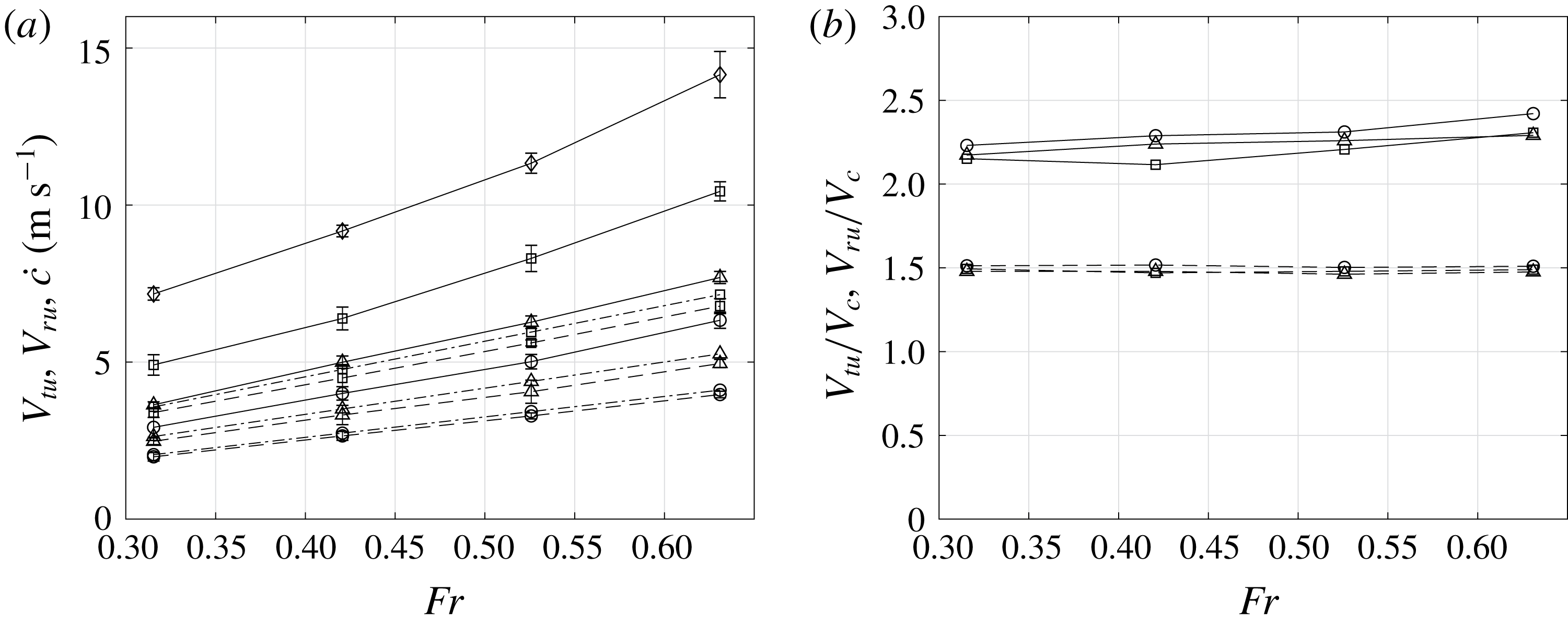
In (a), the horizontal velocities of the under-plate root point (
 $V_{ru}$
) and spray tip (
 $V_{tu}$
) are plotted versus
 $\mathit{Fr}$
for all values of
 $\unicode[STIX]{x1D6FD}$
. In (b),
 $V_{ru}$
and
 $V_{tu}$
scaled by the speed of the geometrical intersection point (
 $V_{c}=W_{0}/\tan \unicode[STIX]{x1D6FD}$
) are plotted versus
 $\mathit{Fr}$
for all values of
 $\unicode[STIX]{x1D6FD}$
. In (a,b), the plot symbols correspond to the value of
 $\unicode[STIX]{x1D6FD}$
(○,
 $\unicode[STIX]{x1D6FD}=25^{\circ }$
; ▵,
 $\unicode[STIX]{x1D6FD}=20^{\circ }$
; ▫,
 $\unicode[STIX]{x1D6FD}=15^{\circ }$
; ♢,
 $\unicode[STIX]{x1D6FD}=10^{\circ }$
) and the line type corresponds to the quantity plotted (——,
 $V_{tu}$
; – – – –,
 $V_{ru}$
; and — ⋅ —, the theoretical prediction of the horizontal velocity of the intersection of the water surface with the bottom surface of the plate by Wagner’s theory, given by
 ${\dot{c}}=(\unicode[STIX]{x03C0}W_{0})/(2\tan \unicode[STIX]{x1D6FD})$
.

The measured horizontal components of the spray tip and root velocities, denoted as
 $V_{tu}$
and
 $V_{ru}$
, respectively, are plotted versus
 $\mathit{Fr}$
in figure 9(a). Both
 $V_{tu}$
and
 $V_{ru}$
increase monotonically with increasing
 $\mathit{Fr}$
and decreasing
 $\unicode[STIX]{x1D6FD}$
. The ratios of the tip and root velocities to the geometric intersection speed,
 $V_{c}=W_{0}/\tan \unicode[STIX]{x1D6FD}$
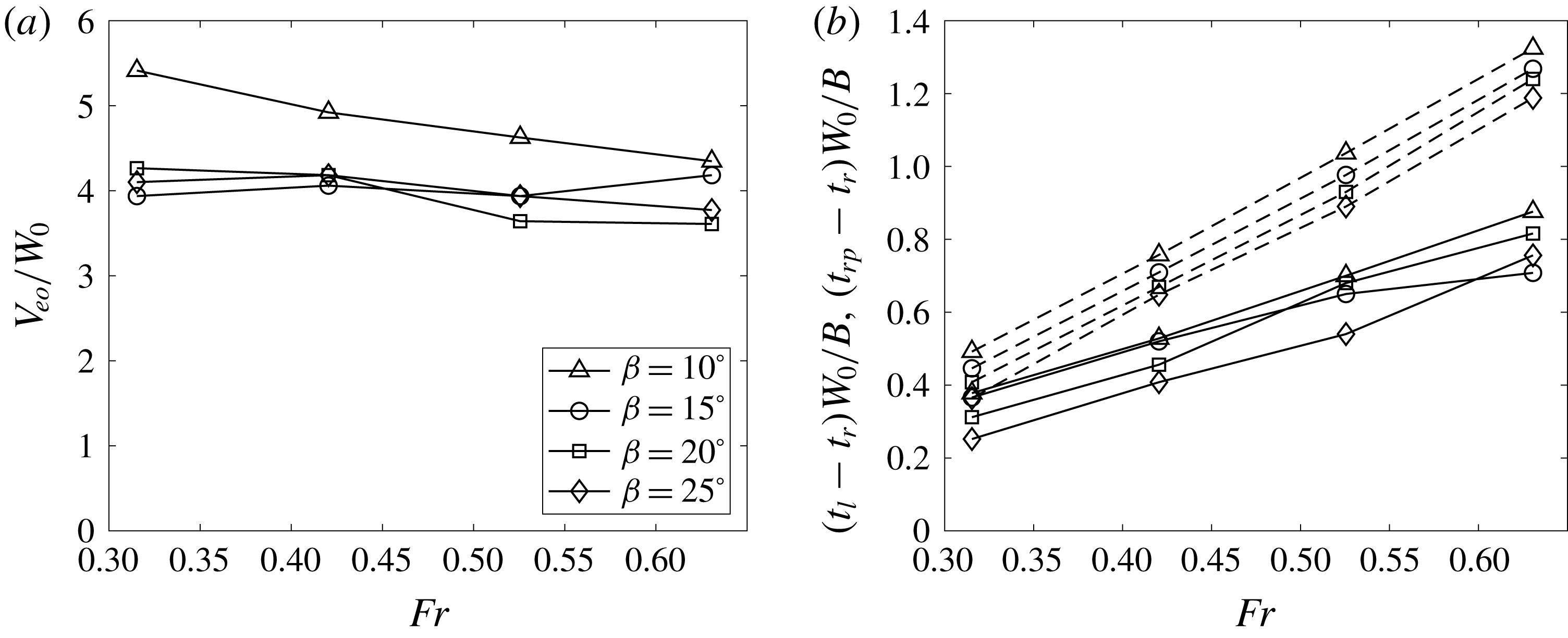
, are plotted in figure 9(b). The root speed ratio
 $V_{ru}/V_{c}$
is found to be nearly independent of
 $\mathit{Fr}$
and
 $\unicode[STIX]{x1D6FD}$
with a value of 1.5. The tip speed ratio is also nearly independent of
 $\mathit{Fr}$
and
 $\unicode[STIX]{x1D6FD}$
with a value of approximately 2.25, i.e. approximately
 $1.5V_{ru}/V_{c}$
. In a simplified analytical model by Wagner (Reference Wagner1932) and also described in Faltinsen (Reference Faltinsen2005, pp. 305–309), the water surface is oriented vertically at the root point. The model does not include the calculation of the spray sheet that is attached to the plate. In this model, the horizontal velocity of the root point is predicted to be
 $$\begin{eqnarray}{\dot{c}}=\frac{\unicode[STIX]{x03C0}W_{0}}{2\tan \unicode[STIX]{x1D6FD}},\end{eqnarray}$$
where
 $c$
is the horizontal distance from the vertex of the wedge to the intersection of the rising water surface and the wedge surface. Thus,
 ${\dot{c}}$
is
 $V_{ru}$
in the present work. The theoretical of value of
 ${\dot{c}}/V_{c}=\unicode[STIX]{x03C0}/2=1.57$
is in close agreement with the present data. The ratio of the measured tip horizontal speed
 $V_{tu}$
to Wagner’s horizontal root speed
 ${\dot{c}}$
is
 $V_{tu}/{\dot{c}}=2.25V_{c}/{\dot{c}}=1.43$
, independent of
 $\unicode[STIX]{x1D6FD}$
. Vincent et al. (Reference Vincent, Xiao, Yohann, Jung and Kanso2018) measured the velocity of the jet tip for wedge deadrise angles between
 $30^{\circ }$
and
 $60^{\circ }$
. The value of the total speed of the jet tip is reported to be
 $1.55{\dot{c}}$
. However, at different deadrise angles, the direction of the jet tip velocity in Vincent et al. (Reference Vincent, Xiao, Yohann, Jung and Kanso2018) is reported to range from
 $18.5^{\circ }$
to
 $39^{\circ }$
from horizontal, resulting in the horizontal speed of the jet tip to be in the range of
 $1.2{\dot{c}}$
to
 $1.47{\dot{c}}$
and this ratio varies with deadrise angle. The lower boundary (at
 $\unicode[STIX]{x1D6FD}=30^{\circ }$
) of this ratio in Vincent et al. (Reference Vincent, Xiao, Yohann, Jung and Kanso2018) is in close agreement with current measurements (
 $10^{\circ }\leqslant \unicode[STIX]{x1D6FD}\leqslant 25^{\circ }$
). In a self-similar potential flow calculation by a fully nonlinear iteration method, Iafrati (Reference Iafrati2012) pointed out that the jet tip speed along the plate follows a
 $1/\unicode[STIX]{x1D6FD}$
trend, i.e. the horizontal speed of the jet tip follows a
 $\cos \unicode[STIX]{x1D6FD}/\unicode[STIX]{x1D6FD}$
trend, in the small
 $\unicode[STIX]{x1D6FD}$
range,
 $\unicode[STIX]{x1D6FD}\leqslant 30^{\circ }$
. The present data agree with this trend qualitatively as
 $V_{tu}\propto \cos \unicode[STIX]{x1D6FD}/\sin \unicode[STIX]{x1D6FD}\approx \cos \unicode[STIX]{x1D6FD}/\unicode[STIX]{x1D6FD}$
when
 $\unicode[STIX]{x1D6FD}$
is small. However, in the calculation, the ratio of the jet tip speed to the impact speed,
 $V_{tu}/W_{0}$
, agrees favourably with
 $3.32/\unicode[STIX]{x1D6FD}$
(where
 $\unicode[STIX]{x1D6FD}$
is in radians), resulting in an estimation of the ratio
 $V_{tu}/{\dot{c}}\approx 2.11$
, when taking
 $\unicode[STIX]{x1D6FD}\approx \sin \unicode[STIX]{x1D6FD}$
. This ratio is larger than that in the present experiments. It is possible that the air resistance acting on the spray and the friction from the plate, which are not considered in the calculation, are responsible for the lower value in the experiment.
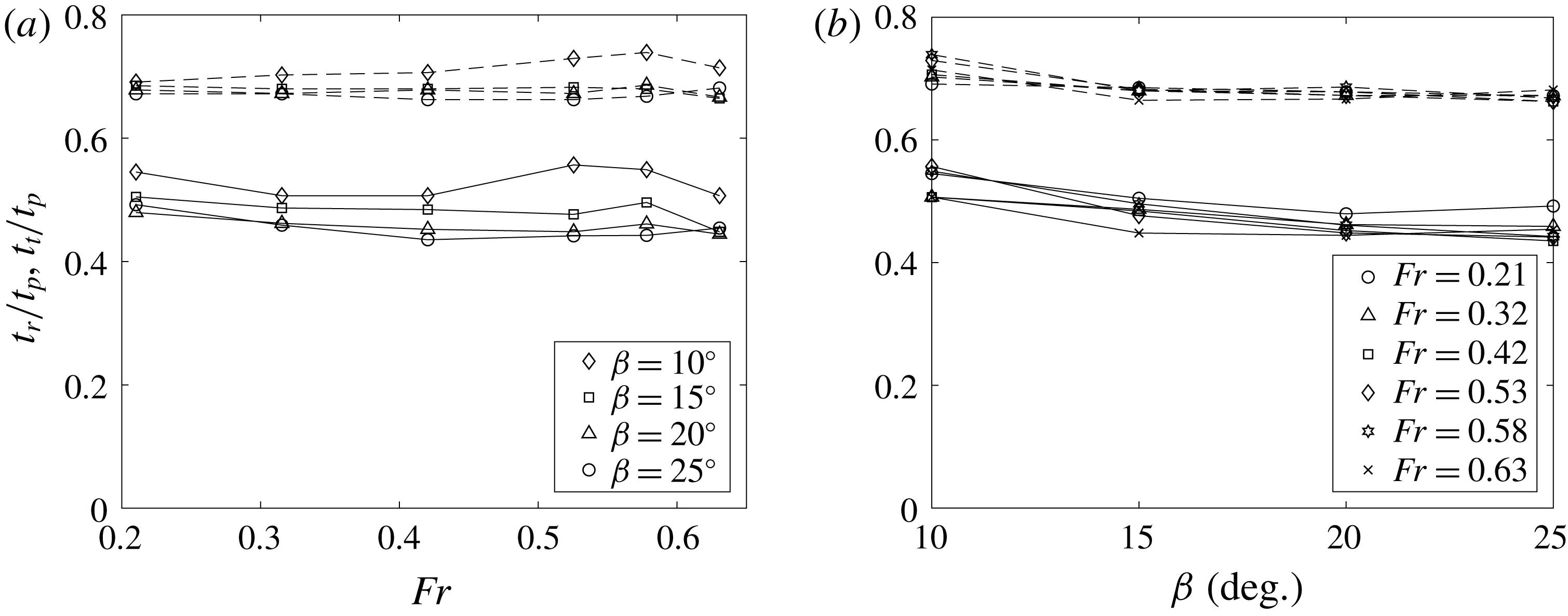
Dimensionless times for the under-plate jet tip (
 $t_{t}/t_{p}$
, ——) and root point (
 $t_{r}/t_{p}$
, – – – –) to propagate from the leading edge to the trailing edge of the plate, where
 $t_{p}$
(
 $=B\sin \unicode[STIX]{x1D6FD}/W_{0}$
) is the time difference between the passage of the leading and trailing edges through the still water level.

Two additional interesting quantities are the time after initial impact (
 $t_{0}=0$
) for the under-plate jet tip and root point to reach the trailing edge of the plate, which are denoted by
 $t_{r}$
and
 $t_{t}$
, respectively. In figure 10, these times, non-dimensionalized by
 $$\begin{eqnarray}t_{p}=\frac{B\sin \unicode[STIX]{x1D6FD}}{W_{0}},\end{eqnarray}$$
the time difference between the passage of the leading and trailing edges of the plate through the still water level, are plotted. As can be seen in the plots, the dimensionless times, are fairly independent of
 $\mathit{Fr}$
and
 $\unicode[STIX]{x1D6FD}$
. The numerical values indicate that
 $$\begin{eqnarray}t_{t}=0.5t_{p}\quad \text{and}\quad t_{r}=0.7t_{p}\end{eqnarray}$$
are good approximations to the data.
3.1.4 Thickness of the spray sheet
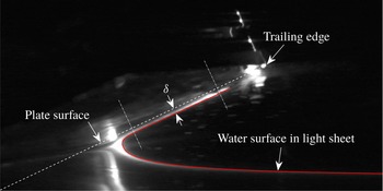
Sample LIF image of the under-plate water surface profile from which the thickness (
 $\unicode[STIX]{x1D6FF}$
) of the spray sheet is found. The solid line is the water surface profile and the dashed line is the plate’s lower surface in the plane of light sheet. The plate surface is extracted from a separate image selected from a high-frame-rate movie that was recorded while the plate was moving in air at a very slow speed. The selection is performed by matching the plate’s position data corresponding to each movie and the match is verified by comparing features in both images. The thickness (
 $\unicode[STIX]{x1D6FF}$
) of the spray sheet is the average of the normal distance between the plate surface and the water surface in the range where this distance is nearly a constant.

The thickness of the under-plate spray sheet can be measured by using the images of the lower surface of the plate and the LIF images of the under-plate spray. After each set of experiments with the same deadrise angle
 $\unicode[STIX]{x1D6FD}$
, the tank water surface was lowered and a movie of the plate motion in air was recorded by the same camera that measures the under-plate spray. The location of the lower surface of the plate in the argon-ion laser sheet plane is recorded. The thickness of the spray sheet is determined by the normal distance from the measured under-plate water surface to the plate’s lower surface. At a fixed time, starting at the under-plate spray root and moving toward the trailing edge, the thickness of the spray sheet first decreases rapidly and then maintains a nearly constant value until near the spray tip, where a thick region forms, see figure 11. The tip region is rough in appearance and ligaments and droplets are ejected under most experimental conditions. Herein, the mean thickness of the spray sheet in the constant range is measured and denoted as
 $\unicode[STIX]{x1D6FF}$
, see figure 11. As discussed in § 3.1.2 and shown in figure 7, for each
 $\unicode[STIX]{x1D6FD}$
, when the under-plate surface profiles are scaled by
 $W_{0}(t-t_{0})$
, they nearly collapse on one curve. Since the plate moves at a constant velocity (
 $W_{0}$
), if one scales the thickness of the under-plate spray sheet by
 $W_{0}(t-t_{0})$
, the scaled thickness at various times is also expected to collapse for each
 $\unicode[STIX]{x1D6FD}$
. Following this idea, the scaled thickness,
 $\unicode[STIX]{x1D6FF}/[W_{0}(t-t_{0})]$
, versus
 $\unicode[STIX]{x1D6FD}$
, is shown in figure 12(a). As can be seen from the figure, the scaled thickness increases with increasing
 $\unicode[STIX]{x1D6FD}$
and is nearly independent of
 $\mathit{Fr}$
at each
 $\unicode[STIX]{x1D6FD}$
. The spread of the data at each
 $\unicode[STIX]{x1D6FD}$
can also be gleaned from the imperfection of the collapse of the scaled profiles in figure 7. This variation is perhaps due to the growing viscous boundary layer along the plate, gravity and difficulty in locating the spray sheet surface due to optical blockage caused by the violent fragmentation of the spray sheet tip into ligaments.
(a) Mean thickness (
 $\unicode[STIX]{x1D6FF}$
) of the under-plate spray sheet, scaled by
 $W_{0}(t-t_{0})$
, versus
 $\unicode[STIX]{x1D6FD}$
. Each symbol in (a) represents the scaled mean thicknesses over various times for each condition and the standard deviation is shown by the error bar. (b) Estimate of the volume of water per unit width in the under-plate spray sheet, scaled by the total volume of water displaced by the plate at this instant (
 $\unicode[STIX]{x1D6FA}_{d}=0.5(\unicode[STIX]{x0394}z)^{2}/\tan \unicode[STIX]{x1D6FD}$
, where
 $\unicode[STIX]{x0394}z=W_{0}(t-t_{0})$
is the depth of penetration below the still water level at this instant). Each symbol in (b) represents the average of
 $\unicode[STIX]{x1D6FA}/\unicode[STIX]{x1D6FA}_{d}$
over various times and the standard deviation is shown by the error bar. In this estimation, the instantaneous distance between the spray tip and root is taken as the length of the spray sheet and the small variation in thickness along the sheet is neglected. The results for case
 $\unicode[STIX]{x1D6FD}=15^{\circ }$
and
 $\mathit{Fr}=0.63$
were not obtained because of difficulties in extracting enough water surface profiles.

The mean thickness of the under-plate spray sheet gives an estimate of the fluid volume per unit span (distance along the plate’s long edges), see figure 12(b). As depicted from the analysis above, at the same
 $\unicode[STIX]{x1D6FD}$
, the velocities of the spray tip and root both scale with
 $W_{0}$
while the thickness scales with
 $W_{0}(t-t_{0})$
. These scalings indicate that the volume of water in the spray sheet scales with
 $W_{0}^{2}(t-t_{0})^{2}$
. Thus, for the same
 $\unicode[STIX]{x1D6FD}$
, the volume of water in the spray sheet,
 $\unicode[STIX]{x1D6FA}$
, scaled by the total volume displaced by the plate,
 $\unicode[STIX]{x1D6FA}_{d}$
, remains approximately constant over time, as indicated in figure 12(b). From the plot, the values of these constants increase with
 $\unicode[STIX]{x1D6FD}$
and vary from approximately 6 % to 12 %. Thus, at every instant, the majority of the displaced water contributes to the rise of the water surface below the under-plate root point as well as a small amount that escapes through the gap between the plate and the symmetry wall.
3.2 Kinematics of the free-surface evolution outboard of the plate’s trailing edge
The free-surface profile evolution outboard of the plate for times after the under-plate root point reaches the plate’s trailing edge,
 $t>t_{r}$
, is discussed in this subsection. This discussion begins with a qualitative description of the surface profile evolution in § 3.2.1, which is followed by four subsections each describing quantitatively, a separate region of the flow. In this subsection, for the convenience of discussion, the position of the plate’s trailing edge at time
 $t=t_{r}$
is defined and referred to as point
 $O(y_{o},z_{o})$
.
3.2.1 Qualitative description of the outboard free surface motion, including feature definitions
Sequence of LIF images of the spray outboard of the plate’s trailing edge for an experimental run with
 $\unicode[STIX]{x1D6FD}=20^{\circ }$
and
 $\mathit{Fr}=0.53$
. The images are taken at a frame rate of 800 pps with a field of view of approximately
 $140~\text{cm}\times 80~\text{cm}$
. The time interval between successive images is 137.5 ms. The image in (a) was taken at the moment when the spray root reached the plate’s trailing edge. These images were taken from supplementary movie 2. Additional movies, taken at the most extreme conditions,
 $\unicode[STIX]{x1D6FD}=10^{\circ }$
,
 $\mathit{Fr}=0.63$
and
 $\unicode[STIX]{x1D6FD}=25^{\circ }$
,
 $\mathit{Fr}=0.21$
are also available as supplementary movies 6 and 7, respectively.

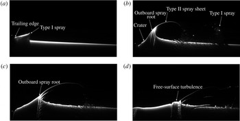
The development of the spray system outboard (to the right) of the plate is illustrated by the sequence of four LIF images of the free surface presented in figure 13 and the corresponding supplementary movie 2. The images are for the case with
 $\unicode[STIX]{x1D6FD}=20^{\circ }$
and
 $\mathit{Fr}=0.53$
; although many aspects of the spray system vary with both
 $\mathit{Fr}$
and
 $\unicode[STIX]{x1D6FD}$
, this case exhibits all the main features. The first image, figure 13(a), was taken at the time when the under-plate root point reached the plate’s trailing edge; at this point in time, the under-plate spray sheet has fully emerged. Just after this instant, the under-plate spray root/spray sheet system passes the plate’s trailing edge and transforms into a wave-like structure with a nearly vertical jet forming from the wave crest region, called herein the outboard spray root, see figure 13(b). As the plate continues to move downward, a crater forms between the plate’s trailing edge and the outboard spray root, see figure 13(b). Similar qualitative behaviour of the spray sheet and crater can be found in the pictures of vertical water entry of a free-falling wedge in Wang et al. (Reference Wang, Lugni and Faltinsen2015b
) and numerically calculated water surface profiles in for example Bao, Wu & Xu (Reference Bao, Wu and Xu2016) and Bao et al. (Reference Bao, Wu and Xu2017). The outboard spray is defined herein as the initially continuous sheet of airborne water between the outboard spray root and the leading edge (tip) of spray that came from the under-plate spray sheet. For convenience, the part of the spray that was originally the under-plate spray sheet is called the Type I spray and the continuous sheet of water moving upward from the outboard spray root is called the Type II spray. Finally, the part of the spray sheet that connects the Type I and II sprays is called the connecting spray. As the impact process continues, the crater deepens and the outboard spray root moves away from the plate, while the Type II spray increases in height. In a typical case as shown in figure 13, the connecting spray sheet quickly breaks up into a region of droplets and ligaments and the Type I and II spray components are separated by the time of image (b). For the later times corresponding to image (c,d), the Type I spray has moved out of the field of view of the camera. Though the Type I spray is initially a continuous sheet of water, it also quickly breaks down into a cloud of droplets and ligaments. Just before the time corresponding to image (d), the wave crest at the outboard spray root forms a weak plunging breaker and the Type II spray begins to fall into the water surface, creating a patch of free-surface turbulent flow as the left edge of the Type II spray continues to move to the right. Between the times corresponding to image (c,d) the crater wall begins to collapse and falls back on the plate.
3.2.2 Characteristics of Type I spray
LIF images of the Type I spray sheet at the instant when the under-plate spray root reaches the trailing edge of the plate for
 $\mathit{Fr}=0.53$
. Images (a–d) are from experimental runs with deadrise angles of
 $\unicode[STIX]{x1D6FD}=10^{\circ }$
,
 $15^{\circ }$
,
 $20^{\circ }$
and
 $25^{\circ }$
, respectively.

The Type I spray is fully emerged from under the plate and appears as a nearly flat sheet of water in the outboard spray LIF images at the time when the under-plate root point reaches the trailing edge, see figure 14. At this instant, the upper free surface along the length of this outboard spray sheet,
 $L_{Io}$
, includes a smooth portion next to the plate’s trailing edge and a rough portion farther outboard, as pointed out in figure 14(d). The transition from smooth to rough free surface may indicate that the boundary layer within the spray sheet transitions from laminar to turbulent flow as fluid particles travel along the length of the plate. The distance travelled by a fluid particle from entry into the spray sheet near the under-plate root point to becoming a free jet at the plate’s trailing edge decreases with time because the under-plate root point moves to the trailing edge. The Reynolds number associated with the largest possible travel distance for a fluid particle, i.e. for a particle that enters the spray sheet at about the time that the leading edge enters the water surface, is approximately
 $\mathit{Re}=V_{tu}B\sec \unicode[STIX]{x1D6FD}/\unicode[STIX]{x1D708}$
and ranges from
 $1.2\times 10^{6}$
to
 $5.5\times 10^{6}$
, which is within the turbulent range for a steady boundary layer on a flat plate in a uniform flow. On the other hand, the Reynolds number for a particle with the shortest possible travel distance, i.e. a fluid particle that enters the spray sheet as the under-plate root point arrives at the trailing edge, is zero. Thus, transition may occur at some place within the spray sheet, at a Reynolds number between these extremes.
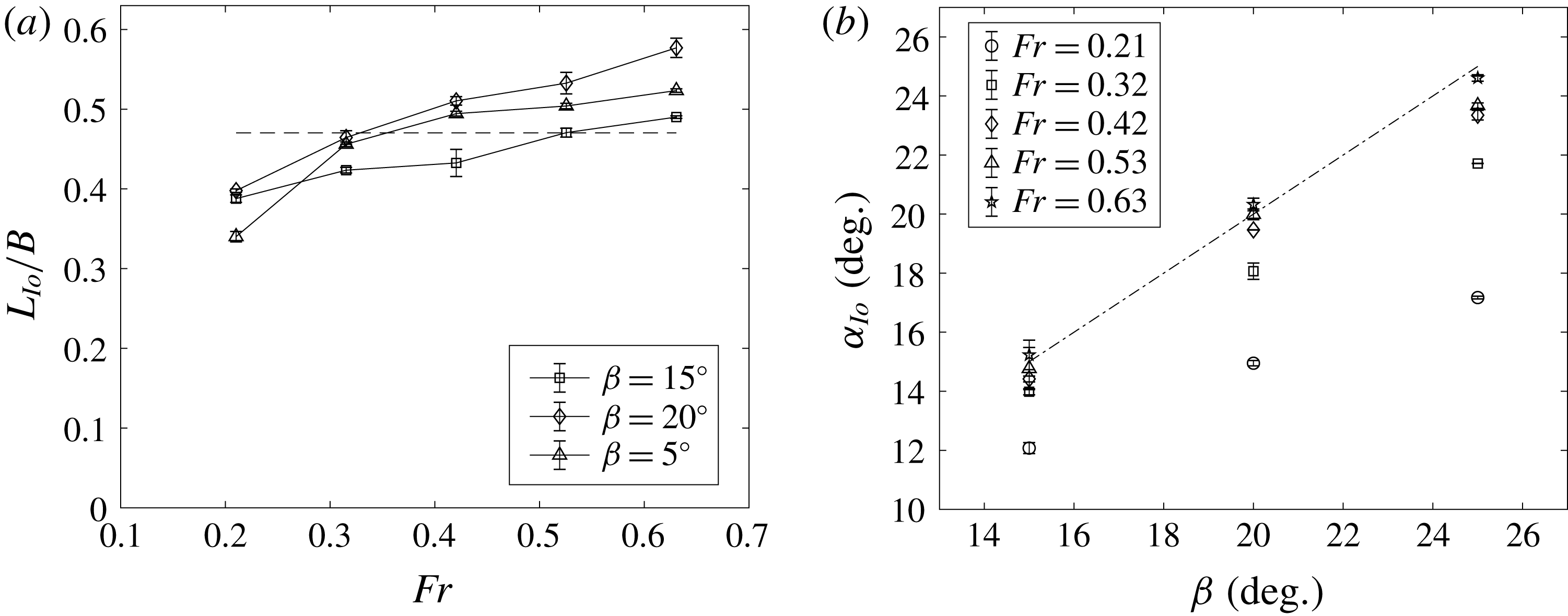
Characteristics of the Type I spray sheet at the instant when the under-plate spray root reaches the plate’s trailing edge (
 $t=t_{r}$
). (a) A plot of the length
 $L_{Io}$
of the spray sheet measured from its tip to the trailing edge of the plate versus
 $\mathit{Fr}$
for
 $\unicode[STIX]{x1D6FD}=15^{\circ }$
,
 $20^{\circ }$
and
 $25^{\circ }$
. The horizontal dashed line is the value of
 $L_{Io}/B$
predicted from the measured values of the speeds and travel times of the under-plate spray tip and root, see text for details. (b) A plot of the angle of inclination of the spray sheet,
 $\unicode[STIX]{x1D6FC}_{Io}$
, versus
 $\unicode[STIX]{x1D6FD}$
for various values of
 $\mathit{Fr}$
. The dash-dotted line is
 $\unicode[STIX]{x1D6FC}_{Io}=\unicode[STIX]{x1D6FD}$
. In both plots, each data point is the mean value over three repeated runs and the error bars are the standard deviations.

At
 $t=t_{r}$
, the Type I spray sheet length
 $L_{Io}$
, measured from the plate’s trailing edge to the spray tip, is plotted versus
 $\mathit{Fr}$
in figure 15(a) for
 $\unicode[STIX]{x1D6FD}=15^{\circ }$
,
 $20^{\circ }$
and
 $25^{\circ }$
. Values of
 $L_{Io}$
for
 $\unicode[STIX]{x1D6FD}=10^{\circ }$
were difficult to obtain because the leading edge of the spray sheet begins to break up into droplets and ligaments before
 $t=t_{r}$
at this value of
 $\unicode[STIX]{x1D6FD}$
. Also, it should be noted that in all cases some of the water at the tip of the spray sheet seems to fall vertically. This effect is most significant in the
 $\mathit{Fr}=0.21$
and
 $\unicode[STIX]{x1D6FD}=25^{\circ }$
case where this falling water reaches the undisturbed water surface at or before
 $t=t_{r}$
, see supplementary movie 3. It is thought that the falling water is composed of the slow moving water in the portion of the boundary layer closest to the plate, which is able to pass through the faster moving water below it only at the spray sheet’s leading edge. The measured values of
 $L_{Io}$
are taken from the above-plate movies; from this camera point of view, the falling water at the spray sheet leading edge is not visible. As can be seen in the plot, the average value of
 $L_{lo}$
is approximately
 $0.45B$
and at the same
 $\unicode[STIX]{x1D6FD}$
, the value of
 $L_{Io}$
increases by from
 $0.1B$
to
 $0.2B$
over the range of
 $\mathit{Fr}$
; however, no obvious trend is found between
 $L_{Io}$
and
 $\unicode[STIX]{x1D6FD}$
. It is also possible to estimate
 $L_{Io}$
from the horizontal component of the under-plate spray sheet tip speed,
 $V_{tu}=1.5V_{c}$
(see figure 9), and
 $t_{r}-t_{t}$
, the difference in time for the under-plate root point and spray sheet tip to reach the trailing edge, see (3.8):
 $$\begin{eqnarray}L_{Io}=\frac{(t_{r}-t_{t})V_{tu}}{\cos \unicode[STIX]{x1D6FD}}\approx 0.47B.\end{eqnarray}$$
This estimated value is in good agreement with the mean value of the measured results in figure 15(a), but it does not show the increasing trend of
 $L_{Io}$
with increasing
 $\mathit{Fr}$
found in the data.
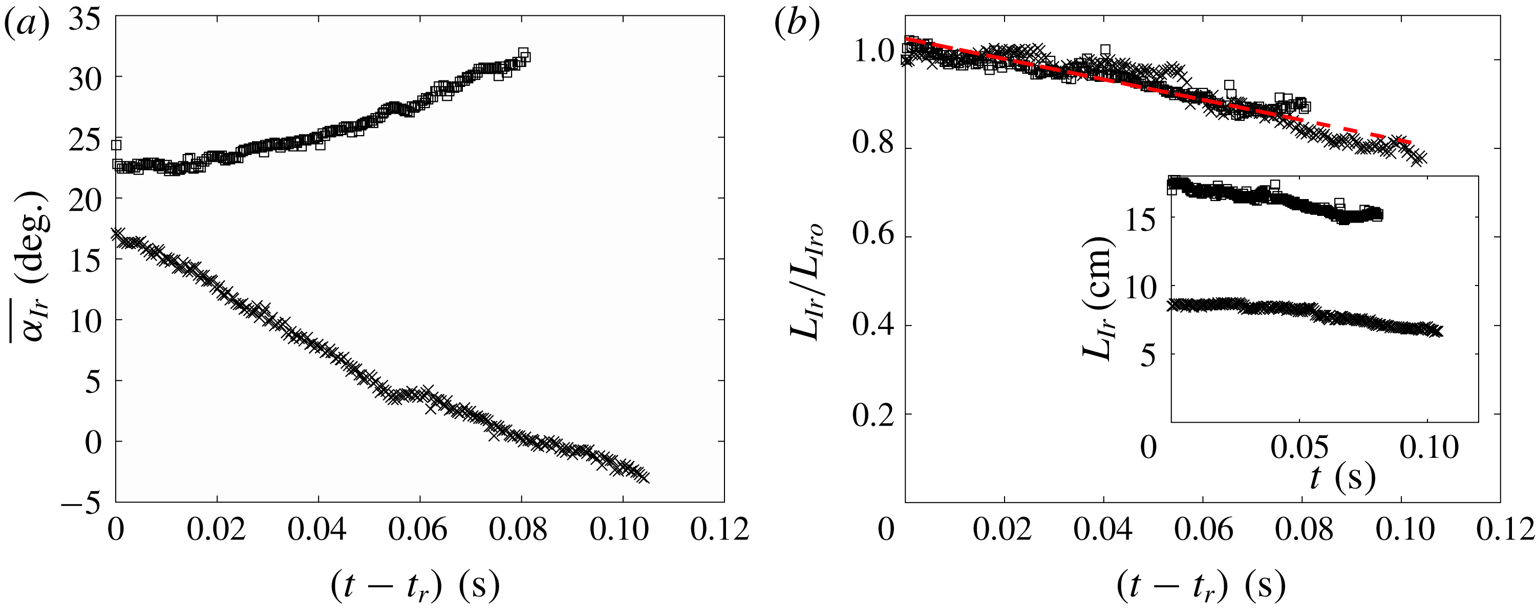
The angle of inclination of the spray sheet
 $\unicode[STIX]{x1D6FC}_{Io}$
at the instant
 $t=t_{r}$
is plotted versus
 $\unicode[STIX]{x1D6FD}$
in figure 15(b). For larger
 $\mathit{Fr}$
, the data tend to the line
 $\unicode[STIX]{x1D6FC}_{Io}=\unicode[STIX]{x1D6FD}$
, the value expected in the absence of gravity. As
 $\mathit{Fr}$
decreases, the data fall farther and farther below the
 $\unicode[STIX]{x1D6FC}_{Io}=\unicode[STIX]{x1D6FD}$
line, indicating that the influence of gravity on the airborne portion of the spray sheet is significant even before the under-plate root point reaches the trailing edge of the plate.
When the under-plate root point first reaches the plate’s trailing edge, the smooth portion of the spray sheet is initially connected to the rough portion. The smooth portion subsequently grows in length and becomes the Type II spray discussed in § 3.2.4. The rough portion of the initial spray sheet becomes the Type I spray. During this latter process, the spray sheet rotates and shrinks in length while moving away from the plate and breaking into a cloud of droplets and ligaments. The initial velocities of the particles (as they pass by the plate’s trailing edge) are thought to be nearly the same and consist of a large component of velocity parallel to the plate (
 ${\approx}2.25W_{0}/\sin \unicode[STIX]{x1D6FD}$
) and a smaller component normal to the plate, equal to
 $W_{0}\cos \unicode[STIX]{x1D6FD}$
. It is thought that without the influence of the air and turbulence in the sheet, the sheet would remain intact and the fluid particles would approximately follow ballistic trajectories. In this simplified scenario, the particle time in free fall is the time since the fluid particle passed by the plate’s trailing edge. Thus, the downward component of the particle velocity and the distance fallen increase as
 $t-t_{t}$
and
 $(t-t_{t})^{2}$
, respectively, and the sheet would rotate, obtaining an increasingly curved (downward) shape as it falls. This effect should increase as the spray sheet formation time,
 $t_{r}-t_{t}$
, increases; as shown in figure 10,
 $t_{r}-t_{t}\approx 0.2B\sin \unicode[STIX]{x1D6FD}/W_{0}$
, i.e. increasing with increasing
 $\unicode[STIX]{x1D6FD}$
and decreasing
 $W_{0}$
(
 $\mathit{Fr}$
).
Top surface profiles of the rough portion of the Type I spray for (a)
 $\mathit{Fr}=0.21$
,
 $\unicode[STIX]{x1D6FD}=25^{\circ }$
and (b)
 $\mathit{Fr}=0.42$
,
 $\unicode[STIX]{x1D6FD}=25^{\circ }$
. The bold curves are the profiles at
 $t=t_{r}$
. For reference, the respective angles of inclination of the bold curves are also shown at the end of the profile sequences by the dash-dotted lines. The still water level and the trailing edge of the plate are located at
 $z/B=0$
and
 $(y-y_{o})/B=0$
, respectively. The time interval between successive profiles is 3.33 ms.

The mean angle of inclination (
 $\overline{\unicode[STIX]{x1D6FC}_{Ir}}$
) and the arc length of the rough portion of the Type I spray sheet (
 $L_{Ir}$
) are plotted versus time in (a) and (b), respectively, for cases
 $\mathit{Fr}=0.21$
,
 $\unicode[STIX]{x1D6FD}=25^{\circ }$
(plotting symbol
 $\times$
) and
 $\mathit{Fr}=0.42$
,
 $\unicode[STIX]{x1D6FD}=25^{\circ }$
(plotting symbol ▫). In (a), the
 $\overline{\unicode[STIX]{x1D6FC}_{Ir}}$
value at each time instant is calculated as the mean of the angle of inclination at each of a uniformly distributed set of interpolation points. In (b), the absolute length
 $L_{Ir}$
for each case is shown in the inset plot, while in the main plot,
 $L_{Ir}$
is scaled by
 $L_{Iro}$
, the value of
 $L_{Ir}$
at
 $t=t_{r}$
. The dashed line, which has a slope of
 $-2.3~\text{s}^{-1}$
, is a linear fit to the data. In both panels,
 $t-t_{r}=0~\text{s}$
is the time when the under-plate root point reaches the plate’s trailing edge.

Type I spray horizontal speed (
 $V_{t}$
) over the plate speed (
 $W_{0}$
) versus distance from the plate’s trailing edge (
 $(y-y_{o})/B$
) for two experimental conditions. The straight lines were computed via least-squares fits to the experimental data.

One influence of air on the motion of the spray sheet is due to lift. Since the spray sheet initially has a positive angle of attack and moves to the right at high speed, the air is expected to induce a counter-clockwise moment, tending to increase the angle of attack. To illustrate the opposing influences of gravity and aerodynamic lift on the motion of the Type I spray sheet, profiles of the rough part of the top surface of the Type I spray sheet are presented for cases with
 $\unicode[STIX]{x1D6FD}=25^{\circ }$
and
 $\mathit{Fr}=$
0.21 and 0.42 in figures 16(a) and 16(b), respectively. For the convenience of comparison, a few profiles before the under-plate root point reaches the trailing edge are also plotted. After the under-plate root point reaches the trailing edge, the spray sheet with the smaller
 $\mathit{Fr}$
, plot (a), rotates clockwise, presumably because the effect of gravity outweighs the effect of aerodynamic lift, while counter clockwise rotation is seen at the higher
 $\mathit{Fr}$
, plot (b), presumably because the lift outweighs the effect of gravity. The mean angle of inclination
 $\overline{\unicode[STIX]{x1D6FC}_{Ir}}$
of the rough parts of the Type I spray sheets versus time is plotted in figure 17(a) for both cases. The decreasing
 $\overline{\unicode[STIX]{x1D6FC}_{Ir}}$
for the lower
 $\mathit{Fr}$
case and increasing
 $\overline{\unicode[STIX]{x1D6FC}_{Ir}}$
for the higher
 $\mathit{Fr}$
case are clearly visible in the plot. The direction of rotation of the Type I spray sheet for all experimental conditions is given in table 1. Clockwise rotation, indicating the dominance of gravity, occurs only in the cases with the lowest Froude number. The length
 $L_{Ir}$
of the rough part of the Type I spray sheet is plotted versus time for the above two cases in figure 17(b). As can be seen in the plot,
 $L_{Ir}$
is larger in the
 $\mathit{Fr}=0.42$
case than in the
 $\mathit{Fr}=0.21$
case for all times plotted. This length decreases with time for both cases and when non-dimensionalized by their initial lengths,
 $L_{Iro}$
, both data sets fall on a single straight line.
The behaviour of the Type I spray later in time, after the spray sheet breaks up and becomes a cloud of droplets, is difficult to quantify. One measure that is possible is the speed of the leading edge of the sheet as determined by measuring the speed of individual droplets. The results of this analysis for two experimental conditions,
 $\mathit{Fr}=0.53$
at two values of
 $\unicode[STIX]{x1D6FD}=15^{\circ }$
and
 $25^{\circ }$
, are shown on a plot of non-dimensional droplet horizontal speed (
 $V_{t}/W_{0}$
) versus non-dimensional horizontal distance from the plate’s trailing edge in figure 18. In both cases, the speed decreases approximately linearly with distance from the plate
 $y$
, probably as a consequence of aerodynamic resistance.
3.2.3 Evolution of the crater
A close-up view of the free-surface profiles in the crater region for
 $\mathit{Fr}=0.53$
. (a–d) Contain profiles for
 $\unicode[STIX]{x1D6FD}=10^{\circ }$
to
 $25^{\circ }$
, respectively. In each plot,
 $y_{o}$
and
 $z_{o}$
are, respectively, the horizontal and vertical coordinates of the plate’s trailing edge at
 $t=t_{r}$
. The time interval between successive profiles is 3.75 ms. The profiles are plotted up to 150 ms after
 $t=t_{r}$
. The horizontal dashed line in each plot is the still water level. The profiles recorded when the plate’s trailing edge reaches the still water level are plotted in bold.

Qualitative classification of the Type I spray sheets according to their direction of rotation, where N denotes neutral (constant slope), CW denotes clockwise (decreasing slope) and CCW denotes counterclockwise (increasing slope).

The width of the crater
 $L_{H}$
(see text for definition) versus time plotted in logarithmic coordinates. (a) Contains the data for deadrise angle
 $\unicode[STIX]{x1D6FD}=20^{\circ }$
and all Froude numbers. In the inset plot, the width
 $L_{H}$
and the time
 $t-t_{r}$
are scaled by
 $B$
and
 $B/W_{0}$
, respectively. In (b),
 $L_{H}/B$
is plotted versus
 $(t-t_{r})W_{0}/B$
in logarithmic coordinates for all experimental conditions. The data are plotted up to the time when the backward propagating surface waves on the crater reaches the trailing edge.

In this subsection, the temporal evolution of the crater will be discussed. In order to compare free-surface profiles and length scales for the various impact conditions, the data are presented in plots with coordinates
 $(y-y_{o},z-z_{o})$
, where
 $O(y_{o},z_{o})$
is defined at the beginning of § 3.2. A set of surface profiles during the expansion of the crater region for
 $\mathit{Fr}=0.53$
and each of the four deadrise angles,
 $\unicode[STIX]{x1D6FD}$
, is shown in figure 19. As discussed above, the plate is moving at constant speed until the trailing edge reaches the still water level; this height and the corresponding crater profile are noted in each plot. Following the top edge of the profile as it moves horizontally, it can be seen that the spacing between profiles, which are equally spaced in time, decreases, indicating that the horizontal speed of expansion is slowing down with time. Following the vertical motion of the bottom edge of the crater, a similar deceleration is seen. The horizontal motion is controlled by the free-surface dynamics, while the vertical motion is controlled by the plate motion, since the lower edge of the crater is always attached to the trailing edge of the plate. It is also noticed that there are ripples generated on the crater surface and these ripples become more prominent as
 $\unicode[STIX]{x1D6FD}$
decreases. It is possible that these ripples come from the small-amplitude oscillations of the plate’s motion around the desired motion profiles. These small-amplitude oscillations are more visible in the small
 $\unicode[STIX]{x1D6FD}$
cases, probably due to the highly transient force acting on the plate; however, the maximum fluctuation of the plate velocity, which is obtained numerically from the plate’s position data, is at most 7 % of the impact velocity in the case with
 $\mathit{Fr}=0.63$
and
 $\unicode[STIX]{x1D6FD}=10^{\circ }$
. Another possibility for the ripple generation is the growth of an instability in the free-surface flow. In any case, these ripple structures do not exist at the upper portion of the crater, where the width of the crater is defined, see discussion below.
In order to compare the crater evolution at the various experimental conditions, the horizontal length
 $L_{H}$
from the origin
 $O$
to the crater surface and the vertical length
 $L_{V}$
from
 $O$
to the bottom of the crater, which is also the trailing edge of the plate, are used. Here,
 $L_{H}$
is chosen as the characteristic length scale of the crater evolution and plotted versus time in figure 20(a) for
 $\unicode[STIX]{x1D6FD}=20^{\circ }$
and all values of
 $\mathit{Fr}$
. The evolution of
 $L_{H}$
seems to follow a power law relation with
 $t$
until near the end of the crater’s growth period for all
 $\mathit{Fr}$
. The exponents of the power law functions at all
 $\mathit{Fr}$
are nearly the same. The magnitude of
 $L_{H}$
at the same time increases with
 $\mathit{Fr}$
, resulting in separate curves for each
 $\mathit{Fr}$
. The increase in the width
 $L_{H}$
is likely due to the larger energy input by the plate’s motion at higher
 $\mathit{Fr}$
over the same period of time. However, if one scales the time by
 $B/W_{0}$
, the data nearly collapse to a single straight line, i.e. a power law function, see the inset plot in figure 20(a). Similarly, the data for all experimental conditions are plotted in these dimensionless coordinates in figure 20(b). The data also form a single straight line and the power law function, as determined by least square fit to the data, is
 $L_{H}/B=0.64[(t-t_{r})W_{0}/B]^{0.77}$
. Dimensional analysis, ignoring the effects of surface tension and viscosity, yields that
 $L_{H}/B$
is potentially a function of only
 $(t-t_{r})W_{0}/B$
,
 $\mathit{Fr}$
and
 $\unicode[STIX]{x1D6FD}$
. The data shown in figure 20(b) indicate
 $\mathit{Fr}$
and
 $\unicode[STIX]{x1D6FD}$
are perhaps not important variables for determining
 $L_{H}$
. The exponent for the present experiments is similar to the value of the scaling exponent used to collapse the surface profiles given in Mayer & Krechetnikov (Reference Mayer and Krechetnikov2018), which were obtained with a very small scale plate with zero deadrise angle and different vertical motion. This later work primarily focuses on the behaviour for very small time, i.e.
 $tW_{0}/B\leqslant 0.01$
. The power law coefficients in both the present experiments and the experiments in Mayer & Krechetnikov (Reference Mayer and Krechetnikov2018) are slightly larger than
 $2/3$
. The
 $2/3$
coefficient was first suggested by Yakimov (Reference Yakimov1973), based on the argument that the flow velocity near the impactor’s edge scales as
 $|r|^{-1/2}$
shortly after the impact, where
 $|r|$
is the distance to the edge of the impactor. This scaling was also suggested by Iafrati & Korobkin (Reference Iafrati and Korobkin2011) and Peters et al. (Reference Peters, van der Meer and Gordillo2013), in studies of the impact of a circular plate on a water surface. This mismatch in the exponents is likely due to the differences between the details of the present experiments and those of these earlier studies.
The angle of inclination of the water surface at the trailing edge of the plate,
 $\unicode[STIX]{x1D703}$
, versus the deadrise angle of the plate,
 $\unicode[STIX]{x1D6FD}$
: ○,
 $\mathit{Fr}=0.21$
; ▫,
 $\mathit{Fr}=0.32$
; ♢,
 $\mathit{Fr}=0.42$
;
 ,
 $\mathit{Fr}=0.53$
; ▹,
 $\mathit{Fr}=0.58$
; ◃,
 $\mathit{Fr}=0.63$
. The dash-dotted line is
 $\unicode[STIX]{x1D703}=\unicode[STIX]{x1D6FD}$
, the condition if the local free surface is parallel to the plate surface at its trailing edge. The length of each error bar is twice the standard deviation of the data at the respective condition.

The angle (
 $\unicode[STIX]{x1D703}$
) relative to horizontal of the tangent to the water surface near the plate’s trailing edge can also be determined from the profiles of the crater. For any combination of
 $\unicode[STIX]{x1D6FD}$
and
 $\mathit{Fr}$
, the experimental data indicate that
 $\unicode[STIX]{x1D703}$
remains nearly constant during the period when the plate is moving at constant speed. The average of
 $\unicode[STIX]{x1D703}$
during this time period is plotted versus
 $\unicode[STIX]{x1D6FD}$
in figure 21. The data indicate that the water surface at the plate’s trailing edge has a steeper slope than that of the plate’s surface, i.e.
 $\unicode[STIX]{x1D703}>\unicode[STIX]{x1D6FD}$
for all experimental conditions. It is worth noting that the measurement of
 $\unicode[STIX]{x1D703}$
shown in figure 21 is based on the surface profile data that resolve features down to 0.4 mm, so micro-scale variations of surface slope with length scale below this minimum are not measurable. As depicted in figure 21,
 $\unicode[STIX]{x1D703}$
does not experience an obvious monotonic trend as
 $\unicode[STIX]{x1D6FD}$
increases. Instead, at
 $\unicode[STIX]{x1D6FD}=15^{\circ }$
,
 $20^{\circ }$
and
 $25^{\circ }$
, the values of
 $\unicode[STIX]{x1D703}$
are nearly the same with a mean value of approximately
 $35^{\circ }$
, while at
 $\unicode[STIX]{x1D6FD}=10^{\circ }$
, the value of
 $\unicode[STIX]{x1D703}$
is approximately
 $30^{\circ }$
. Also, at each
 $\unicode[STIX]{x1D6FD}$
, the value of
 $\unicode[STIX]{x1D703}$
does not have an obvious dependence on the Froude number. The difficulty in obtaining local slopes of the free surface from the measured profiles is likely responsible of the large standard divisions in the plots and may obscure subtle trends in the data. In the experimental study on the impact of a horizontal small plate on a water surface by Mayer & Krechetnikov (Reference Mayer and Krechetnikov2018),
 $\unicode[STIX]{x1D703}$
, therein called the free-surface departing angle, is reported to be larger than the plate’s angle of inclination, which equals to zero. It is worth noting that the flow is assumed to leave the plate surface tangentially in a number of potential flow calculations (see for example, Iafrati & Korobkin Reference Iafrati and Korobkin2004, Reference Iafrati and Korobkin2008). The present results indicate that to accommodate this assumption there would have to be small region (length less than 0.4 mm) of very high surface curvature attached to the plate edge.
3.2.4 Characteristics of the Type II spray
Profiles of the upper free surface of the Type II spray and the crater for
 $\unicode[STIX]{x1D6FD}=10^{\circ }$
and
 $\mathit{Fr}=0.53$
. (a) Shows the surface profiles plotted in a laboratory coordinate system with
 $(y-y_{o})/B=0$
at the plate’s trailing edge and
 $z/B=0$
at the still water level. In (b), the
 $i$
th profile in (a) is shifted vertically by
 $(i-1)\,\text{d}z/B$
where
 $\text{d}z=1~\text{cm}$
. The time between profiles is 7.5 ms. The rough free surface indicated in the plot is due to wave breaking and spray sheet collapse, see text for detailed explanation.

The envelopes of the Type II spray plotted in scaled coordinates for the four deadrise angles are given in (a–d), respectively. Envelopes for all Froude numbers are given in each plot. The envelopes are plotted up to the location where the unstable motion near the top of the spray sheet begins to develop. The location
 $(y_{o},z_{o})$
is the position of the plate’s trailing edge at
 $t=t_{r}$
.

Features of light rays in the imaging process. The side view shows the behaviour of some of the laser light rays; the inset shows in detail the path of laser light rays near the spray root region. Point
 $R$
is at the lower side water surface of the spray sheet, where the surface tangent is vertical. The top view shows light rays from the fluorescing dye in the imaging process. The thick line and arrow in the side view represent the reflected ray that is marked out by the dotted line in the image in figure 25.

In this subsection, the characteristics of the Type II spray sheet and the outboard spray root are discussed. This spray sheet at any instant in time is a streak line composed of fluid that was previously ejected from the outboard spray root, which as is shown below moves both vertically and horizontally after its formation. Two plots of a typical sequence of profiles of the water surface outboard of the plate’s trailing edge for
 $t>t_{r}$
are shown in figure 22. In figure 22(a), the profiles are plotted in a laboratory-fixed reference frame. Early in the sequence, the Type II spray grows rapidly in height while translating away from the plate. The Type II spray has relatively steeper slope near the outboard spray root during this early period and this slope decreases over time and approaches a constant value. Subsequently, the profiles of the Type II spray form nearly parallel curves just before and as the spray sheet collapses on the water surface. A patch of ripples, indicating the possibility of underlying turbulent flow, are generated during the collapse of the spray sheet. In figure 22(b), the same set of surface profiles are shifted vertically over time. A region with high line density approximately represents the propagation of the outboard spray root, which will be discussed in detail later. It should be noted that the spray sheet becomes thin outboard of the point of maximum height, especially at late times, after the spray sheet begins to collapse on the underlying water surface. In addition, in many of the experimental conditions, the spray sheet in this region breaks up into droplets and ligaments. Because of these two phenomena, the surface profile extraction in the above-discussed region is in many cases not possible.
From figure 22(a), it can be seen that the profiles over all time are clearly bounded by a spatial curve, which is herein called the envelope of the Type II spray. Every point below the envelope is at some instant in water and every point above the envelope is always in air. This distinction is significant in that any structural component located below the envelope will be impacted by the spray. Close examination of the profile sequence in figure 22(a) shows that the envelope is created from a sequence of single points, one from each of the Type II spray sheet profiles captured during the time period while the spray sheet is in its growth phase. The envelopes for all experimental conditions are plotted in spatial coordinates scaled by
 $W_{0}^{2}/(2g)$
in figure 23, where a panel with curves for all values of
 $\mathit{Fr}$
is given for each value of
 $\unicode[STIX]{x1D6FD}$
. Before the scaling is performed, the origin of the coordinate system is first shifted vertically to point
 $O$
(
 $y_{o}$
,
 $z_{o}$
), defined at the beginning of § 3.2. This scaling is consistent with dimensional analysis, assuming
 $z=f_{1}(y,W_{0},\unicode[STIX]{x1D6FD},B,g)$
and resulting in
 $$\begin{eqnarray}\frac{zg}{W_{o}^{2}}=f_{2}\left(\frac{yg}{W_{o}^{2}},\unicode[STIX]{x1D6FD},\mathit{Fr}\right).\end{eqnarray}$$
According to figure 23, at
 $\unicode[STIX]{x1D6FD}=10^{\circ }$
and
 $15^{\circ }$
, the envelopes for
 $\mathit{Fr}\geqslant 0.32$
nearly collapse on the same curve while at
 $\unicode[STIX]{x1D6FD}=20^{\circ }$
and
 $25^{\circ }$
, the collapse only appears for envelopes for
 $\mathit{Fr}\geqslant 0.42$
. Thus, the collapse of the envelopes for each
 $\unicode[STIX]{x1D6FD}$
improves with decreasing
 $\unicode[STIX]{x1D6FD}$
and increasing
 $\mathit{Fr}$
. This result serves to help determine the function
 $f_{2}$
in the above equation. Similar deviations from data collapse to a single curve were seen in the analysis of the characteristics of the Type I spray at time
 $t=t_{r}$
, see the plot of the initial angle of inclination of the Type I spray as a function of
 $\unicode[STIX]{x1D6FD}$
in figure 15(b). This similar data collapse behaviour gives some support for the idea that there is a connection between the underplate spray sheet and the ejection of particles into the Type II spray sheet. Indeed, in the under plate LIF movies, it appears that the under-plate spray root converts into the outboard spray root just after
 $t=t_{r}$
.
As mentioned above, the Type II spray sheet consists of fluid particles that were previously ejected at temporally varying initial velocities from the outboard spray root, which moves away from the plate’s trailing edge as the impact proceeds. Thus, the geometry and kinematics of the Type II spray sheet are determined by the flow velocity at the outboard spray root and its trajectory. In view of this connection between the spray root and the Type II spray sheet, the remainder of the current subsection begins with a discussion of the outboard spray root motion and is followed by an estimation of the flow velocity at the outboard spray root.
An LIF image with superposed lines showing the determination of the outboard spray root location. The dashed line represents the upper water surface profile and the dotted line represents the light ray focused by the outboard spray root region as illustrated in figure 24. The filled circle is the intersection of these two lines and is taken as the location of the outboard spray root point.

The trajectories of the outboard spray root point for all
 $\unicode[STIX]{x1D6FD}$
are shown in each panel: (a)
 $\mathit{Fr}=0.21$
, (b)
 $\mathit{Fr}=0.32$
, (c)
 $\mathit{Fr}=0.42$
, (d)
 $\mathit{Fr}=0.53$
, (e)
 $\mathit{Fr}=0.58$
, (f)
 $\mathit{Fr}=0.63$
. In all plots,
 $y_{r}-y_{o}=0$
is at the horizontal location of the plate’s trailing edge and
 $z_{r}=0~\text{cm}$
is at the still water level.

Trajectories of the outboard spray root point for all
 $\mathit{Fr}$
are plotted in each panel: (a)
 $\unicode[STIX]{x1D6FD}=10^{\circ }$
, (b)
 $\unicode[STIX]{x1D6FD}=15^{\circ }$
, (c)
 $\unicode[STIX]{x1D6FD}=20^{\circ }$
, (d)
 $\unicode[STIX]{x1D6FD}=25^{\circ }$
. In all plots,
 $y_{r}-y_{o}=0$
is at the horizontal location of the plate’s trailing edge and
 $z_{r}=0~\text{cm}$
is at the still water level.

Horizontal velocities of the outboard spray root point for all
 $\mathit{Fr}$
are plotted in each panel: (a)
 $\unicode[STIX]{x1D6FD}=10^{\circ }$
, (b)
 $\unicode[STIX]{x1D6FD}=15^{\circ }$
, (c)
 $\unicode[STIX]{x1D6FD}=20^{\circ }$
, (d)
 $\unicode[STIX]{x1D6FD}=25^{\circ }$
.

Vertical velocities of the outboard spray root point for all
 $\mathit{Fr}$
are plotted in each panel: (a)
 $\unicode[STIX]{x1D6FD}=10^{\circ }$
, (b)
 $\unicode[STIX]{x1D6FD}=15^{\circ }$
, (c)
 $\unicode[STIX]{x1D6FD}=20^{\circ }$
, (d)
 $\unicode[STIX]{x1D6FD}=25^{\circ }$
.

The LIF images of the outboard spray when the plunging jet of the breaker is visible. (a,b) Show the camera view from above and below the spray sheet, respectively. Both images are taken 309 ms after
 $t=t_{r}$
for
 $\unicode[STIX]{x1D6FD}=25^{\circ }$
,
 $\mathit{Fr}=0.53$
. Images (a,b) were taken from supplementary movies 4 and 1, respectively..

As defined in § 3.2.1, the outboard spray root is a small region at the crest of the wave-like structure that propagates away from the plate as the impact proceeds. In order to quantify the motion of the outboard spray root, we define, somewhat arbitrarily, the root point based on our LIF images of the outboard spray, in the following manner. Within the outboard spray root region, the slope of the lower side air–water interface transitions from negative to positive, see figure 24. At a certain point in the region (point
 $R$
in figure 24), the local water surface is vertical. The light-sheet optics above the tank create input laser light rays that are then refracted at the upper side air–water interface. Most refracted rays travel within the water phase and illuminate the subsurface water that is mixed with fluorescent dye. These refracted rays form the background illumination for qualitatively observing water surface features that are between the light-sheet plane and the camera. One refracted ray that reaches point
 $R$
from the water phase is reflected internally by the local air–water interface. As shown in the inset of figure 24, when the local upper side interface (
 $IF_{U}$
) is at an angle
 $\unicode[STIX]{x1D703}_{1}$
from the horizontal direction and the input ray is at an angle
 $\unicode[STIX]{x1D703}_{2}$
from the vertical direction, according to Snell’s law, the incident angle (
 $\unicode[STIX]{x1D703}_{3}$
) of the refracted ray on the lower side interface (
 $IF_{L}$
) at point
 $R$
can be expressed as
 $$\begin{eqnarray}\unicode[STIX]{x1D703}_{3}=90^{\circ }-\unicode[STIX]{x1D703}_{1}+\arcsin \left[\frac{n_{a}\sin (\unicode[STIX]{x1D703}_{1}-\unicode[STIX]{x1D703}_{2})}{n_{w}}\right],\end{eqnarray}$$
where
 $n_{a}=1$
and
 $n_{w}=1.3$
are the index of refraction of air and water, respectively. The input rays are nearly vertical in the present experiments, i.e.
 $\unicode[STIX]{x1D703}_{2}\approx 0^{\circ }$
. The angle (
 $\unicode[STIX]{x1D703}_{1}$
) between the local upper side interface and the horizontal direction ranges from approximately
 $45^{\circ }$
to
 $80^{\circ }$
at different
 $\unicode[STIX]{x1D6FD}$
values. Thus, according to (3.11),
 $\unicode[STIX]{x1D703}_{3}$
ranges from
 $58^{\circ }$
to
 $77^{\circ }$
. The critical incident angle for total internal reflection at the air–water interface is
 $49^{\circ }$
. Therefore, at the lower side interface near point
 $R$
, total internal reflection occurs and all the energy is reflected toward the water phase. This reflected ray crosses with the other rays refracted by the upper air–water interface. As a result, the laser light is focused to form a bright ‘line’ with high light intensity in the water phase in the plane of light sheet. This bright ‘line’ becomes a subsurface light source and the light that originates along this bright ‘line’ is then refracted by the upper water–air interface (crater surface) and some of this light enters the lens of the camera. Since the curvature of the crater surface is small and the camera lens has a long focal length, the image that the bright ‘line’ casts on the camera sensor remains nearly a straight line, as shown in the LIF image in figure 25. This bright ‘line’ is extended to intersect with the upper surface profile of the Type II spray. Since the thickness of the Type II spray is very small, this intersection point is a good representation of the position of the outboard spray root region and is herein called the outboard spray root point, see figure 25. The appearance and behaviour of this bright ‘line’ are very consistent over time. At the moment when the Type II spray starts to fall down on the water surface, this ‘line’ is at the position of the starting point of the free-surface splash zone, further indicating it is a consistent and faithful representation of the outboard spray root.
With the above-described method, the trajectories of the outboard spray root point were determined and are shown in figures 26 and 27. As is shown figure 26, where a plot containing trajectories for all values of
 $\unicode[STIX]{x1D6FD}$
is given for each
 $\mathit{Fr}$
, the trajectories for each
 $\unicode[STIX]{x1D6FD}$
nearly collapse to a single curve. In particular, the maximum heights of the trajectories are nearly independent of
 $\unicode[STIX]{x1D6FD}$
, while at both ends of the trajectories, the slopes increase and the heights decrease only slightly as the values of
 $\unicode[STIX]{x1D6FD}$
decrease. It is interesting that in contrast to this root point behaviour, the envelopes of the Type II spray change dramatically with
 $\unicode[STIX]{x1D6FD}$
, see figure 23. In figure 27, the root point trajectory data are shown in four plots, with each plot containing the trajectories for one value of
 $\unicode[STIX]{x1D6FD}$
and all values of
 $\mathit{Fr}$
. As depicted in the figure, at the same value of
 $\unicode[STIX]{x1D6FD}$
, the trajectories for all Froude numbers follow a nearly straight line starting from the plate’s trailing edge. As
 $\mathit{Fr}$
is increased, the trajectories follow this line to a larger
 $(y-y_{o})/B$
and the maximum height of the trajectories increases.
From examination of the LIF movies taken of the region outboard of the plate’s trailing edge, the outboard spray root region appears to behave like the crest of a gravity wave generated by the impulsive motion of the plate. To further explore this concept, the horizontal velocities of the outboard spray root point at all experimental conditions are plotted in figure 28. In all cases, the horizontal velocity of the outboard root point,
 $V_{r}$
, decreases quickly, from approximately
 $2.5~\text{m}~\text{s}^{-1}$
to approximately
 $1.0~\text{m}~\text{s}^{-1}$
within approximately 0.07 s, as the root point leaves the plate’s trailing edge. According to studies of the water entry of a wedge (for example, Zhao & Faltinsen Reference Zhao and Faltinsen1993) there is a high-pressure zone travelling with the under-plate spray root. The sudden decrease in speed of the outboard spray root point is probably related to the emergence of the high-pressure zone from the plate edge at
 $t=t_{r}$
. Subsequently,
 $V_{r}$
approaches a nearly constant value of approximately
 $1.0~\text{m}~\text{s}^{-1}$
for all
 $\unicode[STIX]{x1D6FD}$
and
 $\mathit{Fr}$
. By the linear dispersion relationship for a deep-water gravity wave, the length of a wave with a phase speed of
 $c_{p}=1.0~\text{m}~\text{s}^{-1}$
is
 $\unicode[STIX]{x1D706}=2\unicode[STIX]{x03C0}c_{p}^{2}/g=0.64~\text{m}\approx 1.7B$
. These data support the idea that the plate impact is impulsive, selecting a wavelength proportional to the width of the plate rather than the plate’s impact speed. The vertical velocity of the outboard root point is plotted versus time in figure 29, where a plot of the data for all values of
 $\mathit{Fr}$
is given for each
 $\unicode[STIX]{x1D6FD}$
. The data in each plot nearly collapse to a single curve that starts at approximately
 $2~\text{m}~\text{s}^{-1}$
and decreases almost linearly, after an initial period, with a downward acceleration almost equal to the acceleration of gravity. After the outboard spray root point reaches its maximum height, the spray root region appears to undergo a process similar to a plunging breaking wave crest, see the LIF images in figure 30. As the breaking continues, the bottom end of the Type II spray sheet begins to collapse and a rough surface patch is generated by a combination of the breaking wave and the collapsing spray sheet.
Geometrical constraints on the magnitude (
 $V_{e}$
) and angle (
 $\unicode[STIX]{x1D719}_{e}$
) of the velocity of fluid particles emerging from the outboard spray root. At an arbitrary instant
 $t_{a}$
, the fluid particle position
 $P_{a}$
and the outboard spray root
 $R_{a}$
coincide. After a short time
 $\unicode[STIX]{x0394}t$
(
 $\unicode[STIX]{x0394}t\ll 1$
), the fluid particle moves to a position
 $P_{b}$
on the spray sheet and the root moves to
 $R_{b}$
.

As mentioned above, the time history of the fluid particle velocity at the outboard spray root and the motion of the spray root determine the development and behaviour of the Type II spray sheet. While the motion of the root point was measured as described above, the fluid velocity measurement was not attempted. In the following, the measured spray sheet profiles and the outboard root point trajectories are used with a ballistic model of the airborne spray sheet to estimate the fluid velocity at the root point. In this simple model, the effects of the surrounding air, surface tension and viscosity are neglected. Similar ideas with different configurations have been applied to the analysis of ejecta generated under different scenarios (see for example, Thoroddsen et al. Reference Thoroddsen, Thoraval, Takehara and Etoh2011; Vincent et al. Reference Vincent, Xiao, Yohann, Jung and Kanso2018).
The model and its connection to the measured data are described as follows. The magnitude (
 $V_{e}$
) and angle (
 $\unicode[STIX]{x1D719}_{e}$
) of the emerging fluid particle velocity at the root point at any instant must satisfy the following geometrical constraint:
 $$\begin{eqnarray}(V_{e}\cos \unicode[STIX]{x1D719}_{e}-V_{r})\tan \unicode[STIX]{x1D719}_{s}=V_{e}\sin \unicode[STIX]{x1D719}_{e}-W_{r},\end{eqnarray}$$
as shown in figure 31, where
 $V_{r}$
and
 $W_{r}$
are the horizontal and vertical velocity of the outboard root point, respectively, as given in figures 28 and 29. The angle
 $\unicode[STIX]{x1D719}_{s}$
is the instantaneous angle of inclination of the spray sheet at the outboard root point, which is determined from the measured surface profiles of the Type II spray.
The position
 $(y_{p},z_{p})$
at any time
 $t$
of a fluid particle that was ejected from the root point at
 $t_{e}$
with speed
 $V_{e}$
and angle
 $\unicode[STIX]{x1D719}_{e}$
is determined by the following equations:
 $$\begin{eqnarray}\displaystyle & y_{p}(t)=y_{p}|_{t=t_{e}}+V_{e}|_{t=t_{e}}\cos \unicode[STIX]{x1D719}_{e}|_{t=t_{e}}(t-t_{e}), & \displaystyle\end{eqnarray}$$
 $$\begin{eqnarray}\displaystyle & z_{p}(t)=z_{p}|_{t=t_{e}}+V_{e}|_{t=t_{e}}\sin \unicode[STIX]{x1D719}_{e}|_{t=t_{e}}(t-t_{e})-{\textstyle \frac{1}{2}}g(t-t_{e})^{2}, & \displaystyle\end{eqnarray}$$
where
 $(y_{p}|_{t=t_{e}},z_{p}|_{t=t_{e}})$
is also the position of the root point
 $(y_{r},z_{r})$
at
 $t=t_{e}$
. All the fluid particles that emerged from the outboard root point prior to the current instant make up the current spray profile. To simplify the problem,
 $V_{e}(t)$
is assumed to follow an exponential form, as suggested by Vincent et al. (Reference Vincent, Xiao, Yohann, Jung and Kanso2018). In particular, in the present model, it is assumed that
 $$\begin{eqnarray}V_{e}(t)=V_{eo}\exp \left[\frac{t-t_{r\prime }}{t_{l}-t_{r\prime }}\ln \left(\frac{V_{el}}{V_{eo}}\right)\right],\end{eqnarray}$$
where
 $V_{eo}$
is the emerging speed of the first fluid particle ejected from the spray root at
 $t=t_{r\prime }$
and
 $t_{r\prime }$
is taken slightly after
 $t_{r}$
since the first few measured profiles after
 $t=t_{r}$
are too small to have enough resolution to accurately satisfy the geometrical constraints (shown in figure 31),
 $V_{el}$
and
 $t_{l}$
are the speed and ejection time of the last fluid particle that emerges from the root point, respectively. At
 $t=t_{l}$
, the speed of the fluid particle equals the speed of the outboard root point, i.e.
 $$\begin{eqnarray}V_{el}=\sqrt{V_{r}|_{t=t_{l}}^{2}+W_{r}|_{t=t_{l}}^{2}},\end{eqnarray}$$
which can be determined from the measured root point velocities as long as
 $t_{l}$
is known. Thus, the objective of the model is to find the optimal values of
 $V_{eo}$
and
 $t_{l}$
such that the instantaneous coordinates of the fluid particles
 $(y_{p},z_{p})$
computed from (3.13) and (3.14) are as close as possible to the experimentally measured spray profiles. By minimizing the average offset between the measured and the simulated spray envelopes, the optimal values of
 $V_{eo}$
and
 $t_{l}$
were determined and are presented in figure 32. The streak lines of the fluid particles computed by the above-described model using the optimal parameters are plotted together with measured surface profiles of the Type II spray sheet in figure 33 for two typical conditions. As depicted in figure 33, the envelopes of the spray sheet from the simulation agree satisfactorily with those from the experiments and the model successfully captures the shape of each Type II spray sheet up to its location of maximum height. A rough estimation of the emerging speed of fluid particles at the outboard spray root is given by this simplified model, as shown in figure 32(a), where a curve is given for each
 $\unicode[STIX]{x1D6FD}$
. It is thought that the departure of the
 $\unicode[STIX]{x1D6FD}=10^{\circ }$
curve from the other three curves, may be the effect of the early breakup of the Type II spray sheet, which is observed for the
 $\unicode[STIX]{x1D6FD}=10^{\circ }$
conditions, on the ballistic computation. According to this prediction,
 $V_{eo}$
is approximately four times of the vertical impact velocity,
 $W_{0}$
, for all values of
 $\mathit{Fr}$
at the three larger values of
 $\unicode[STIX]{x1D6FD}$
. At
 $\unicode[STIX]{x1D6FD}=10^{\circ }$
, the ratio between
 $V_{eo}$
and
 $W_{0}$
is approximately 5. The estimated results indicate
 $V_{eo}$
perhaps scales with
 $W_{0}$
, not the speed of the geometrical intersection,
 $V_{c}$
. The estimated duration of the fluid particle emerging process,
 $t_{l}$
, is plotted in figure 32(b), as is the time when the first surface ripple is generated due to the sheet collapse and wave breaking in the experiments. According to the model prediction, the emerging process stops before the first surface ripple is seen in the experiments. This result is consistent with the idea that the ripple generation occurs as the fluid particles in the spray sheet fall onto the water surface below.
(a) Initial emerging speed (
 $V_{eo}$
) of fluid particles at the spray root as estimated by the model and scaled by
 $W_{0}$
versus
 $\mathit{Fr}$
. (b) The time (
 $t_{l}$
) when fluid particles stop emerging from the outboard spray root point as estimated by the model and scaled by
 $B/W_{0}$
versus
 $\mathit{Fr}$
(solid lines). The dashed lines in (b) represent the time (
 $t_{rp}$
) when the first free-surface ripple is generated according to observations of the high-speed LIF movies.

Type II spray surface profiles from experiments and the simulation for two typical cases with
 $\mathit{Fr}=0.42$
. (a,b) Correspond to
 $\unicode[STIX]{x1D6FD}=15^{\circ }$
and
 $20^{\circ }$
, respectively. The profiles are plotted up to the instant when fluid particles stop emerging from the outboard spray root in the simulation. Each experimental profile is plotted from the spray root to a point where the horizontal position is 3 cm past the horizontal location of the maximum height of the spay sheet.

3.2.5 Connecting spray: separation mechanism of Type I and Type II sprays
In this subsection, the connecting spray between the Type I and II sprays is discussed. In the typical case described in § 3.2.1, the connecting spray breaks up, resulting in a complete separation between the Type I and II sprays. By qualitative examination of the LIF movies of all cases, it is found that the connecting spray tends to break up early at large
 $\mathit{Fr}$
and small
 $\unicode[STIX]{x1D6FD}$
. To illustrate this tendency, LIF images taken at two typical instants from four experimental conditions with different values of
 $\unicode[STIX]{x1D6FD}$
and the same
 $\mathit{Fr}=0.53$
are presented in figure 34. The images in (a) were taken at the instant when the plate’s trailing edge reached the still water level. As depicted in (a), the connecting spray remains continuous for
 $\unicode[STIX]{x1D6FD}=20^{\circ }$
and 25
 $^{\circ }$
, while it just begins to break up into ligaments for
 $\unicode[STIX]{x1D6FD}=15^{\circ }$
. For
 $\unicode[STIX]{x1D6FD}=10^{\circ }$
, the Type I and II sprays are clearly separated. In (b), the LIF images were taken 50 ms after the instant shown in (a). At this later time, separation of the Type I and Type II spray also occurs for
 $\unicode[STIX]{x1D6FD}=20^{\circ }$
, while the connecting spray for
 $\unicode[STIX]{x1D6FD}=25^{\circ }$
is still in the process of stretching. As is also depicted in figure 34, and in agreement with the above-discussed speeds of the Type II spray root and the Type I spray, the distance travelled by the Type I spray over the 50 ms time period significantly increases as
 $\unicode[STIX]{x1D6FD}$
decreases, while the distance travelled by the Type II spray is shorter and does not vary significantly with
 $\unicode[STIX]{x1D6FD}$
. For convenience in describing this effect quantitatively, the characteristic speed of the Type II spray is chosen as the horizontal speed of the outboard root point while the characteristic speed of the Type I spray is chosen as the horizontal speed of the under-plate spray tip as it emerges from under the plate. As discussed above, the speed of the root point of the Type II spray is nearly the same for all conditions (
 ${\approx}1~\text{m}~\text{s}^{-1}$
), as shown in figure 28, while the speed of the Type I spray is
 $2.25W_{0}/\tan \unicode[STIX]{x1D6FD}$
, which ranges from 1.9 to
 $15.0~\text{m}~\text{s}^{-1}$
, see figure 9. Contours of the difference between these characteristic speeds (
 $\unicode[STIX]{x1D6FF}U$
) are plotted on a
 $\mathit{Fr}$
–
 $\unicode[STIX]{x1D6FD}$
plane in figure 35. Data points indicating the connecting spray behaviour, as observed in the high-speed LIF movies, coarsely define the boundary between the non-separation and separation regimes. This boundary is clearly aligned well with the contours.
LIF images of the outboard spray system for four deadrise angles and
 $\mathit{Fr}=0.53$
. In the column of images on the left (ai–aiv), the plate’s trailing edge is at
 $z=0~\text{cm}$
while the images in the column on the right (bi–biv) were taken 50 ms after the respective image in column (a). The rows of two images from (i) to (iv) correspond to deadrise angles of
 $\unicode[STIX]{x1D6FD}=10^{\circ }$
,
 $15^{\circ }$
,
 $20^{\circ }$
and
 $25^{\circ }$
, respectively. The movies from which these images were taken have been complied into a single movie, supplementary movie 5.

Another potential mechanism for the breakup of the connecting spray is due to the surrounding air flow. In the study of the water entry of a small wedge with large deadrise angles by Vincent et al. (Reference Vincent, Xiao, Yohann, Jung and Kanso2018), it is pointed out that the surrounding air flow creates a pressure difference between the upper and lower sides of the spray sheet. To explore this possibility in the present experiments, the following discussion will focus on the kinematics of the connecting spray’s lowest point, near which the breakup of the connecting spray first occurs. The vertical position of the lowest point,
 $z_{k}$
, versus time is shown in figure 36(a) for a number of experimental conditions. The
 $z_{k}$
versus
 $t$
curves are approximately parabolic functions. The vertical velocities of the lowest point,
 $w_{k}$
, are calculated by numerically differentiating the
 $z_{k}$
versus
 $t$
data and are shown in figure 36(b). As depicted in the plot, the variation of vertical acceleration (the slope of the curves in plot (b)) is not sensitive to
 $\mathit{Fr}$
. However, the vertical acceleration is found smaller in cases with the larger
 $\unicode[STIX]{x1D6FD}$
. For
 $\unicode[STIX]{x1D6FD}=25^{\circ }$
, the vertical acceleration is slightly larger than
 $g$
while a vertical acceleration of approximately
 $10g$
is found for
 $\unicode[STIX]{x1D6FD}=10^{\circ }$
. The highest accelerations are found just before the spray sheet breaks up. High vertical accelerations at the lowest point on the connecting spray ranging from
 $10g$
to
 $90g$
are reported in Vincent et al. (Reference Vincent, Xiao, Yohann, Jung and Kanso2018). This large acceleration on the connecting spray, likely induced by the air flow, probably facilitates the breakup of the connecting spray.
Regimes of separation between the Type I and Type II sprays. The grey level represents the difference (
 $\unicode[STIX]{x1D6FF}U$
) in the horizontal speeds of the Type I and II sprays, as defined in § 3.2.5. The connecting spray behaviour, as seen in the LIF movies, is indicated by the plot symbols: ●, the connecting spray sheet remains continuous; ▪, connecting spray sheet breaks up; ○, the connecting spray behaviour falls on the boundary between the two regimes; and ▹, the connecting spray impinges on the water surface before breaking up.

The vertical position and velocity of the lowest point on the connecting spray sheet are shown in (a) and (b), respectively. The values of
 $\unicode[STIX]{x1D6FD}$
are given by the colour and the values of
 $\mathit{Fr}$
are denoted by the plot symbol, as given in the figure legend. The vertical position and velocity are measured up to the instant when the Type I and II sprays separate.

4 Conclusions
An experimental study of the spray formation during the vertical impact of a tilted rectangular flat plate (length
 $L=1.22~\text{m}$
, width
 $B=0.38~\text{m}$
) on a quiescent water surface is performed for tilt angles
 $\unicode[STIX]{x1D6FD}$
ranging from
 $10^{\circ }$
to
 $25^{\circ }$
and Froude numbers,
 $\mathit{Fr}=W_{0}/\sqrt{gB}$
, ranging from 0.21 to 0.63, where
 $W_{0}$
is the plate’s impact velocity and
 $g$
is the gravitational acceleration. The plate motion, which is driven by a servo motor with programmable control system, is set to maintain a constant speed until the trailing (upper) long edge of the plate passes the still water level (SWL) and then to decelerate to a stop.
The spray formation begins with the rise of the water surface and the generation of a thin spray sheet under the plate as the plate’s leading edge touches the still water surface. It is found that the under-plate surface profiles at different times nearly collapse on a single curve when scaled by
 $W_{0}t$
and the collapsed profiles are in agreement with the similarity solution proposed by Dobrovol’Skaya (Reference Dobrovol’Skaya1969) and calculated in Wang & Faltinsen (Reference Wang and Faltinsen2017). The horizontal velocity of the tip of the under-plate spray sheet is about 2.25 times the speed of the geometrical intersection between the plate’s bottom surface and the still water surface (
 $V_{c}$
) for all conditions. The horizontal velocity of the under-plate root point is approximately
 $1.5V_{c}$
and is nearly equal to the growth rate of the wet length in Wagner’s theory. The under-plate spray structure emerges from the plate’s trailing edge and subsequently forms the outboard spray system. The outboard spray system is categorized into Type I spray, the crater adjacent to the plate’s trailing edge, the Type II spray, and the connecting spray. The Type I spray comes from the under-plate spray sheet, travelling with initial speeds as high as
 $15~\text{m}~\text{s}^{-1}$
. It then decelerates, rotates and shrinks in length as it moves under the combined effect of gravity and aerodynamic force. The crater is generated as the plate’s trailing edge hits the local water surface. The bottom of the crater is attached to the plate’s trailing edge and the crater width (
 $L_{H}$
) expands as the plate continues to move downward. The growth of the crater’s width is found to follow a non-dimensional power law relationship,
 $L_{H}/B=0.64((t-t_{r})W_{0}/B)^{0.77}$
, which is independent of
 $\unicode[STIX]{x1D6FD}$
. Also, for all experimental conditions, the angle of inclination of the local water surface at the plate’s trailing edge is found to be larger than
 $\unicode[STIX]{x1D6FD}$
(to the resolution of the present measurements). The Type II spray is a thin sheet of water and it’s root is initially located at the crater’s upper edge. At moderate and high
 $\mathit{Fr}$
, for each
 $\unicode[STIX]{x1D6FD}$
the envelopes of the Type II spray collapse on a single curve when scaled by
 $W_{0}^{2}/(2g)$
. During the spray sheet generation process, the outboard spray root behaves like the crest of an impulsively generated and freely propagating wave. The horizontal velocity of the outboard root point (wave crest) is nearly the same for all conditions, indicating that the wavelength is selected primarily by the plate width, which is held constant in these experiments. The connecting spray between the Type I and II sprays tends to break up into ligaments and droplets for large
 $\mathit{Fr}$
and small
 $\unicode[STIX]{x1D6FD}$
. Two possible stretching mechanisms are thought to be responsible for this break up. The first stretching mechanism is caused by the large difference between the speeds of the Type I and II sprays. The second mechanism is due to the large local vertical acceleration near the lowest point on the connecting spray. The large acceleration, which was as high as
 $10g$
for selected conditions, is probably due to unsteady air motion as discussed in Vincent et al. (Reference Vincent, Xiao, Yohann, Jung and Kanso2018), where accelerations as high as
 $90g$
were found in experiments performed with
 $30^{\circ }\leqslant \unicode[STIX]{x1D6FD}\leqslant 60^{\circ }$
and
 $2.0\leqslant \mathit{Fr}\leqslant 6.0$
.
Acknowledgement
A.W. and J.H.D. gratefully acknowledge the support of the Office of Naval Research (grant N000141612619, program manager Dr S. Russell).
Supplementary movies
Supplementary movies are available at https://doi.org/10.1017/jfm.2019.630.