





Impact Statements
This study focuses on statistical methods to reveal trends in noisy experimental data gathered for thermally aged rubber. The methods are statistical hypothesis tests of the data and model selection. Statistical hypothesis tests of experimental data do not require a quantitative model. Consequently, their results are not affected by modeling assumptions. A disadvantage is that they often cannot consider all experimental data. To ensure that all data can be considered, model selection can be applied. The downside of model selection is that only a limited number of quantitative models are assessed against the data. Because each method compensates for the other’s shortcomings, statistical tests of data and model selection together offer a rigorous platform to detect trends in scattered data.
1. Introduction
Rubber can react with different chemicals in its environment (Layer and Lattimer, Reference Layer and Lattimer1990; Song et al., Reference Song, Liang, Wang, Song, Tian, Qiang, Tian and Chen2024). If rubber is surrounded by air, oxygen diffuses into the rubber (Celina et al., Reference Celina, Wise, Ottesen, Gillen and Clough1998) and causes chain scission and cross-link formation (Cunneen, Reference Cunneen1968; Han et al., Reference Han, Wu, Quan and Niu2020; Wei et al., Reference Wei, Xie, He, Zhu, Liu, Zhang and Liao2022). These two processes occur continuously and explain why rubber’s fracture stress degrades over time, and the modulus increases over time. For an increase in temperature, the processes accelerate and consequently, so does the evolution of mechanical properties (Celina et al., Reference Celina, Gillen and Assink2005). Consequently, many mechanical frameworks for elastomers incorporate temperature and oxidative aging (Behnke and Kaliske, Reference Behnke and Kaliske2015, Reference Behnke and Kaliske2018; Lejeunes et al., Reference Lejeunes, Delattre, Eyheramendy, Méo and Ahose2018; Bouaziz et al., Reference Bouaziz, Ahose, Lejeunes, Eyheramendy and Sosson2019; Cruanes et al., Reference Cruanes, Deffarges, Lacroix and Méo2019; Le Mouellic et al., Reference Le Mouellic, Charlès, Le Cam, Boyard, Bailleul, Gaudry and Veillé2021; Redon et al., Reference Redon, Le Cam, Robin, Miroir and Fralin2023).
The general consensus accepts a monotonic relation between the aging temperature and the evolution rate of mechanical properties: the higher the aging temperature, the faster the properties evolve. This entails that a property can degrade or grow, but not both. Most aging models, such as those based on time-temperature-superposition, intrinsically incorporate this monotonic relation (Huang and Kinloch, Reference Huang and Kinloch1993; Zhu et al., Reference Zhu, Jiang, Cheng, Zhang, Guo, Xiong, Fu, Yang and Jiang2015; Tao et al., Reference Tao, Shen, Chen, Liu, Gao, Wu and Tsige2018).
1.1. Aim
However, the fracture stress of the peroxide-cured EPDM of interest to this study seems to both degrade and grow, depending on the aging temperature. Because fracture stress growth conflicts with the general consensus and because the experimental data exhibit substantial scatter, the aim of this study was to demonstrate the use of two probabilistic concepts to quantitatively investigate fracture stress growth in detail. The two methods are model-free statistical hypothesis tests and model selection. They have hardly been, if ever, applied in the field of elastomer research—to the best of the authors’ knowledge. Therefore, this study could facilitate the adoption of data-driven and statistical approaches within the elastomer community.
The focus on the fracture stress is motivated by different reasons. First, the fracture stress normally only degrades due to thermal aging, but here it can also improve—an atypical and therefore interesting phenomenon. Second, the fracture stress is often studied to assess the impact of thermal aging (Ning et al., Reference Ning, Ma, Zhang, Zhang, Wu and Tian2014; Öncel et al., Reference Öncel, Gül, Efe, Erdoğan and Karaağaç2023). Third, fracture stress measurements often exhibit considerable noise, making it difficult to distinguish trends with the naked eye. Fourth, fracture stress measurements are closely related to fracture toughness measurements. Therefore, the qualitative relation between thermal aging and the fracture toughness in phase-field damage models for elastomers (Loew et al., Reference Loew, Peters and Beex2019, Reference Loew, Peters and Beex2020a, Reference Loew, Poh, Peters and Beex2020b; Yin and Kaliske, Reference Yin and Kaliske2020) can follow a similar qualitative relation as that between the fracture stress and thermal aging.
Despite this study’s focus on the evolution of the fracture stress due to thermal oxidative aging, the application of the two methods (i.e., model-free statistical hypothesis tests and model selection) can be applied to any material property and any physical mechanism, for example, the number and length of cracks due to ozone attack, modulus change due to thermal aging, and surface embrittlement due to photo-oxidation. The application of the methods to the fracture stress should thus be considered as a demonstrative example only.
1.2. Statistical hypothesis tests without model assumptions
The statistical hypothesis tests (Lieber, Reference Lieber1990; Guyatt et al., Reference Guyatt, Jaeschke, Heddle, Cook, Shannon and Walter1995) are directly applied to the experimental data. They are used to investigate whether the fracture stress degrades for a certain aging temperature, remains the same for a certain aging temperature, or grows for a certain aging temperature. The advantage of these tests is that they investigate the experimental data directly. Hence, they do not need an aging model, which is intrinsically associated with model assumptions.
The model-free statistical hypothesis tests investigate whether two sets of data are statistically equivalent (i.e., the difference between the two datasets is only caused by random chance alone) or statistically different (i.e., the difference between the two datasets is caused by a statistically significant, underlying effect). The tests accomplish this by quantifying the probability that two datasets originate from the same distribution (with the same distribution parameters). This probability is quantified by the p-value (Goodman, Reference Goodman2008; Thiese et al., Reference Thiese, Ronna and Ott2016; Lakens, Reference Lakens2021). A large p-value indicates a high probability that the two datasets originate from the same distribution, whereas a small p-value indicates the opposite, that is, some statistically significant, underlying effect is responsible for the difference between the two datasets.
Although a tiny p-value indeed indicates a high probability that two datasets originate from two different distributions, it does not provide any information about how different these two distributions are. To quantify the difference between the two distributions from which each dataset originates, another metric must be used. This study uses the effect size for this purpose (Ferguson, Reference Ferguson2009; Kelley and Preacher, Reference Kelley and Preacher2012; Tomczak and Tomczak, Reference Tomczak and Tomczak2014).
This study applies two statistical tests to the experimental data: the two-tailed (Wilcoxon) Mann–Whitney U test (MWU test) (Mann and Whitney, Reference Mann and Whitney1947; Fay and Proschan, Reference Fay and Proschan2010; MacFarland and Yates, Reference MacFarland and Yates2016) and the two-sample Smirnov test (Hodges, Reference Hodges1958; Berger and Zhou, Reference Berger and Zhou2014), which is more widely known as the two-sample Kolmogorov–Smirnov test (KS test). The tests are readily available in different software packages (e.g., Python’s SciPy library, Matlab, SPSS, R). They can even be performed online (see e.g., Statskingdom’s MWU test, 2025 for the MWU test and Statskingdom’s KS test, 2025 for the KS test). Both tests have their own advantages and downsides.
The conventional two-tailed MWU test (Mann and Whitney, Reference Mann and Whitney1947; Fay and Proschan, Reference Fay and Proschan2010; MacFarland and Yates, Reference MacFarland and Yates2016) is suited for small datasets, bounded data, and is nonparametric. The latter issue means that the MWU test does not assume that the data of each set originates from a specific distribution. Because the datasets are relatively large for the conventional MWU test, the test statistic is assumed to behave according to a normal distribution (Siegel, Reference Siegel1956). This approximation implies that the employed MWU test does not neatly incorporate the fact that the data are bounded. The MWU test only investigates the central tendency of the data. All these aspects make the MWU test highly suited to analyze fracture stress data.
The two-sample KS test (Hodges, Reference Hodges1958; Berger and Zhou, Reference Berger and Zhou2014; Finner and Gontscharuk, Reference Finner and Gontscharuk2018) investigates both the central tendency and the shape of the distributions that underlie the datasets. Similar to the employed MWU test, the KS test is nonparametric. However, the KS test incorporates the fact that the data are bounded—in contrast to the employed variant of the MWU test. Whereas the datasets are rather large for the original MWU test (and consequently, the MWU variant with a normal approximation is applied), the datasets are, in some instances, relatively small for the KS test. By applying both the MWU test and the KS test, a comparison can be made since both tests are based on different concepts and investigate different aspects.
The advantage of applying statistical tests directly to experimental data is that no aging model is required and, hence, their results are unaffected by modeling assumptions. However, the tests also come with a disadvantage if they are applied to properties that evolve over time. The problem involves the selection of the two datasets. To investigate whether the fracture stress degrades, remains the same, or grows over time at a certain aging temperature, the fracture stress data of unaged rubber are gathered in the first set. The fracture stress data recorded for the longest aging duration (at a specific aging temperature) are gathered in the second set. The reason is that the fracture stress hardly changes for short aging durations (see ahead to Figure 5). However, by only comparing the fracture stress data of unaged rubber with those of rubber aged for the longest duration, a substantial amount of data is ignored.
1.3. Model selection
To ensure that all experimental data are incorporated in the quantitative assessment, model selection is applied to several aging models that account for the time-dependent change in the fracture stress. Model selection provides a ranking that quantitatively assesses the suitability of the different aging models (Zucchini, Reference Zucchini2000; Stoica and Selen, Reference Stoica and Selen2004; Ding et al., Reference Ding, Tarokh and Yang2018).
Model selection is stricter than the model-free statistical hypothesis tests. The reason is that even if the statistical hypothesis tests indicate that the fracture stress degrades and grows for different aging temperatures, model selection can still indicate that the additional model complexity necessary to incorporate growth outweighs the improvement in accuracy.
The underlying concept of model selection is Occam’s razor (Domingos, Reference Domingos1999; Forster, Reference Forster2000; Stoffi et al., Reference Stoffi, Cevolani and Gnecco2022). The principle assumes that the simplest model that explains the real-world observations is most likely the most suitable model. Model selection can be performed with different information criteria (Burnham and Anderson, Reference Burnham and Anderson2004; Stoica and Selen, Reference Stoica and Selen2004). These criteria consist of a cost function and a profit function. The cost function quantifies the complexity of each model by means of the number of model parameters. The profit function quantifies the accuracy of each model.
This study applies model selection by means of the Akaike information criterion (AIC) (Akaike, Reference Akaike1974) and the Bayesian information criterion (BIC) (Schwarz, Reference Schwarz1978). The reasons for applying these two criteria are that they are the best-known criteria and by applying two criteria instead of one, a comparison can be made. Both the AIC and the BIC use the same profit function, but a different cost function. Its practical implication is that the BIC favors model simplicity more than the AIC (Burnham and Anderson, Reference Burnham and Anderson2004).
Model selection as applied in this study (i.e., using parameter values deterministically calibrated using least-squares) is strictly speaking not a statistical hypothesis test, but model selection based on the Bayes factor does constitute genuine hypothesis testing (Kass and Raftery, Reference Kass and Raftery1995; Hoijtink et al., Reference Hoijtink, Mulder, Van Lissa and Gu2019). However, the application of the Bayes factor requires the probabilistic identification of the model parameters (Rappel et al., Reference Rappel, Wu, Noels and Beex2019, Reference Rappel, Girolami and Beex2022; Zeraatpisheh et al., Reference Zeraatpisheh, Bordas and Beex2021), and a smaller audience is familiar with probabilistic identification and/or Bayesian inference than with deterministic least-squares identification. On top of that, calculating the Bayes factor goes one step further than the probabilistic identification, since it also requires dedicated techniques such as bridge sampling (Gronau et al., Reference Gronau, Sarafoglou, Matzke, Ly, Boehm, Marsman, Leslie, Forster, Wagenmakers and Steingroever2017; Wang et al., Reference Wang, Jones and Meng2022) or thermodynamical integration (Gelman and Meng, Reference Gelman and Meng1998; Liu et al., Reference Liu, Elshall, Ye, Beerli, Zeng, Lu and Tao2016; Mingo et al., Reference Mingo, Nijzink, Ley and Hale2025) to compute the marginal likelihood. On the other hand, it may be noted that the BIC and Bayes factor are closely related (Raftery, Reference Raftery1999; Weakliem, Reference Weakliem1999; Ibrahim et al., Reference Ibrahim, Chen and Sinha2001).
1.4. Context
Although the true aim of this study was a demonstration of the use of statistical hypothesis tests and model selection in the field of elastomer research, the statement that the fracture stress of the rubber of interest both degrades and grows as a result of thermal oxidative aging deserves to be placed in a bit more context. The reason is that the general consensus is that the fracture stress only degrades due to thermal oxidative aging. However, the EPDM rubber of interest here is peroxide-cured instead of being vulcanized by sulfur, as is the case with the majority of rubbers. In fact, two previous studies have also reported an aging-induced growth of the fracture stress for peroxide-cured EPDMs (Ning et al., Reference Ning, Ma, Zhang, Zhang, Wu and Tian2014; Öncel et al., Reference Öncel, Gül, Efe, Erdoğan and Karaağaç2023).
Another factor that comes into play is the aging duration. In the current study, a maximal aging duration of 72 days is applied. It could very well be that for longer aging durations, the fracture stress also degrades for aging temperatures for which growth is observed in the current study. However, the maintenance policy of the authors’ industrial collaborator advises replacing its rubber parts after months rather than years. This justifies why the current study focuses on relatively short aging times. On the other hand, the maximal aging duration in the current study is 72 days, whereas Ning et al. (Reference Ning, Ma, Zhang, Zhang, Wu and Tian2014) and Öncel et al. (Reference Öncel, Gül, Efe, Erdoğan and Karaağaç2023) use maximal aging durations of 9 days and 14 days, respectively.
1.5. Outline
The remainder of this study is organized as follows. The next section briefly summarizes the experimental campaign but focuses in more detail on the two-tailed MWU test and two-sample KS test. Section 3 summarizes a number of aging models that are subjected to model selection as discussed in Section 4. Section 5 presents the results, and Section 6 presents some conclusions.
2. Statistical hypothesis testing of the data
This section starts with a discussion of the sample preparation and testing procedure. The second subsection discusses the application of the MWU test and the KS test.
2.1. Sample preparation and testing
The specimen preparation follows the same manufacturing process as the industrial partner uses for its products. The compound of the peroxide-cured EPDM is protected by intellectual property and is unknown to the authors.
The industrial partner does not produce the EPDM rubber, but does perform the vulcanization step (achieved by peroxide). To this end, sheets of 125
$ \times $
 100
$ \times $
 2 mm
$ {}^3 $
 are cut from EPDM rubber plies as received. Each sheet is then placed in a compression mold with a pressure of 20 MPa for 15 minutes at 170 °C to achieve vulcanization. Afterward, the sheets are stored at
$ 23\pm 3 $
 °C for at least 24 hours. The mass of each sheet is 30.92 grams (with a standard deviation of 0.14 gram). The reported glass transition temperature is around −75 °C.
Subsequently, dog bone specimens are cut from a sheet, all with the same orientation. The specimens are then thermally aged according to ISO 11346:2014. The ovens are designed for long-term aging and may experience temperature deviations of 3 °C. The specimens are hung from metallic rods without mutual contact and contact with the oven walls. The ovens ventilate regularly, yielding oxidative aging. Thermal oxidative aging is applied for a maximum aging duration of 72 days, for temperatures of 50 °C, 60 °C, 70 °C, 90 °C, 120 °C, 140 °C, and 150 °C. At regular intervals, specimens are taken out of the oven for uniaxial testing. Specimens are allowed to cool down for a minimum of 24 hours.
Uniaxial tensile tests are performed according to ISO 37:2017 with a Zwick/Roell tensile tester. The effective area of each specimen is measured individually. Two markers are attached to the specimens to measure the stretch during the tensile experiment with an optical extensometer that employs two lasers. The temperature during uniaxial testing is
$ 23\pm 3 $
 °C.
2.2. Model-free statistical hypothesis tests
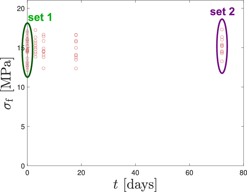
The two model-free statistical hypothesis tests require the selection of two sets of data. Figure 1 illustrates this selection for the data recorded for an aging temperature of 120 °C. Naturally, the first set consists of the fracture stress data of unaged rubber. The second set consists of fracture stress data of rubber that is aged for the longest duration at a specific aging temperature (although sets at some other aging durations are also selected in the results section).
Experimental fracture stresses (red circles) recorded for aging at 120 °C as a function of the aging duration. The two sets of fracture stress data are encircled. The first set (green) envelopes all the data of unaged rubber. The second set (purple) envelopes all the data of rubber aged for the longest duration, that is, 72 days.

Figure 1. Long description
A scatter plot with the horizontal X-axis labeled t [days] ranging from 0 to 80 and the vertical Y-axis labeled sigma sub f [M P a] ranging from 0 to 20. Red open circles represent individual data points.
* At t equals 0, a dense vertical cluster of data points is encircled by a green oval labeled set 1. These points are concentrated between 12 and 18 M P a.
* Moving right, smaller clusters of data points appear at approximately 3, 6, and 18 days, maintaining a similar vertical spread.
* At the far right of the plot, at t equals 72 days, a final vertical cluster of data points is encircled by a purple oval labeled set 2. These points are also concentrated between 13 and 18 M P a, showing no significant downward trend in fracture stress over the 72-day period.
2.3. Two-tailed Mann–Whitney U test with normal approximation
Considering set 1 with
$ {n}_1 $
 data points and set 2 with
$ {n}_2 $
 data points, the MWU test (Mann and Whitney, Reference Mann and Whitney1947; MacFarland and Yates, Reference MacFarland and Yates2016) starts by merging the fracture stress data from both sets in a single list and sorting the list in ascending order. The sorted list of length
$ {n}_1+{n}_2 $
 provides a ranking of all data points, where the index of each data point serves as the rank of said data point. Subsequently, the ranks of all data points in set 1 are summed, resulting in the rank sum of set 1,
$ {R}_1 $
 . The same is performed for set 2, which yields rank sum
$ {R}_2 $
 . Next, the U-statistic for each set is calculated according to:

with
$ i=\left\{1,2\right\} $
 .
Next, the smallest of the two U-statistics is selected and denoted by
$ U $
 . With
$ U $
 available, the Z-score, which quantifies how many standard deviations
$ U $
 is removed from the mean, can be calculated according to:

with the following mean and standard deviation:

Here, the U-statistic is assumed to be normally distributed (Siegel, Reference Siegel1956) because
$ {n}_1 $
 and
$ {n}_2 $
 are relatively large for the data in this study in relation to the MWU test. Nevertheless, the MWU test remains nonparametric, because the assumption of normality applies to the ranks of the data and not to the raw data. On the other hand, the fact that the fracture stress data are bounded is not incorporated due to the normal approximation.
Next, the two-tailed p-value is calculated with the help of the Z-score:

where
$ N\left(a,{b}^2\right) $
 denotes the normal distribution with mean
$ a $
 and standard deviation
$ b $
 , and erf(
$ \bullet $
 ) denotes the erf function.
Finally, the standardized effect size is calculated according to
$ Z $
 /
$ \sqrt{n_1+{n}_2} $
 .
2.4. Two-sample Kolmogorov–Smirnov test
The application of the two-sample KS test (Hodges, Reference Hodges1958; Berger and Zhou, Reference Berger and Zhou2014) starts with the construction of the empirical cumulative distribution functions (eCDFs) of the two sets, here denoted by
$ {\hat{F}}_1\left({\sigma}_{\mathrm{f}}\right) $
 and
$ {\hat{F}}_2\left({\sigma}_{\mathrm{f}}\right) $
 for sets 1 and 2, respectively. The eCDF of set 1 can be written as:

with:

where
$ {\underline {\tilde{\sigma}}}_{\mathrm{f}}^1 $
 stores set 1’s fracture stress data in ascending order and
$ {\tilde{\sigma}}_{\mathrm{f}/i}^1 $
 denotes the
$ {i}^{\mathrm{th}} $
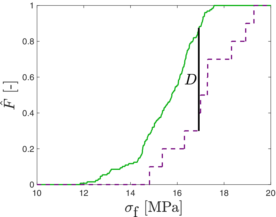
 fracture stress measurement in set 1. In the same way, the eCDF of set 2 must also be constructed. Figure 2 presents a graphical illustration of two potential eCDFs, where set 1 (green, solid) contains many more data points than set 2 (purple, dashed).
Illustration of an eCDF for set 1 (green, solid) and one for set 2 (purple, dashed). The test statistic
$ D $
 , that is, the maximum vertical distance between the two eCDFs, is presented as a black solid line. The eCDFs are not associated with the data in Figure 1.

Figure 2. Long description
The horizontal x axis is labeled sigma sub f in units of M P a, ranging from 10 to 20. The vertical y axis is labeled F hat, ranging from 0 to 1. Two step-like curves represent the e C D Fs.
* The first curve, a solid green line, begins its ascent at approximately 12 M P a and reaches 1 at roughly 17.5 M P a.
* The second curve, a dashed purple line, begins its ascent later at approximately 14.8 M P a and reaches 1 at roughly 19.5 M P a.
A thick black vertical line segment is positioned at approximately 17 M P a. This segment spans the vertical gap between the dashed purple line at y equals 0.3 and the solid green line at y equals 0.88. The letter D is placed to the left of this vertical line to indicate the test statistic for the maximum vertical distance.
Next, the maximal vertical distance between the two eCDFs is calculated:

where
$ D $
 denotes the KS test statistic (see Figure 2).
Subsequently, matrix
$ \underline {\underline{C}} $
 of size
$ \left({n}_1+1\right)\times \left({n}_2+1\right) $
 is constructed, with components
$ {C}_{i,j} $
 at the
$ {i}^{\mathrm{th}} $
 row and the
$ {j}^{\mathrm{th}} $
 column calculated as follows:

and the p-value is given by the component
$ {C}_{n_1,{n}_2} $
 . Hence, the p-value is calculated exactly in this study (Viehmann, Reference Viehmann2021), but often Smirnov’s approximation is used (Hodges, Reference Hodges1958; Marsaglia et al., Reference Marsaglia, Tsang and Wang2003).
The effect size is quantified by
$ D $
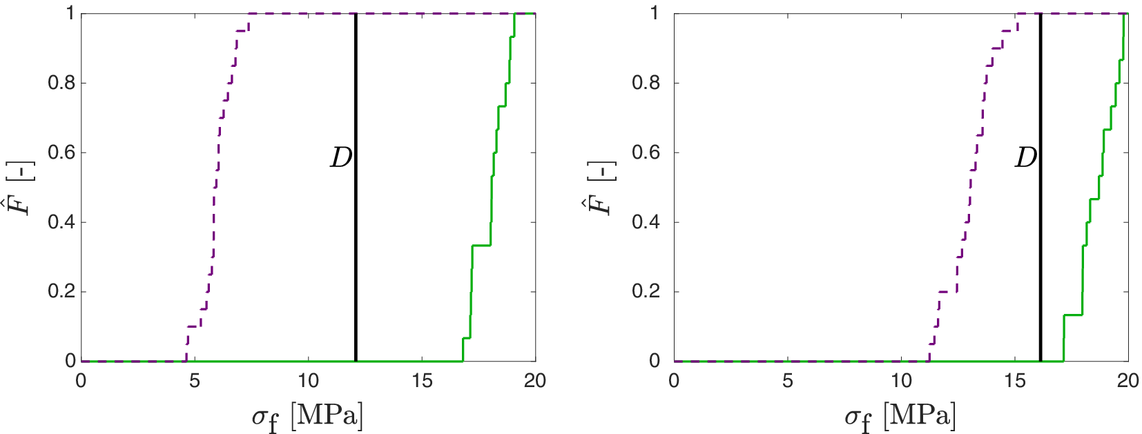
 . This comes with the disadvantage that the effect size does not change for widely varying datasets. This is illustrated in Figure 3. The eCDFs in the left diagram clearly differ more than the two eCDFs in the right diagram, but
$ D=1 $
 for both cases. Thus, the KS test cannot quantify the effect size for widely varying datasets and will always yield an effect size of 1 in those cases.
Two cases for which the effect size of the two-sample KS test is the same (
$ D=1 $
 ), whereas the two eCDFs in the left diagram are clearly more different than the two in the right diagram.

3. Aging models
Similar to most model-free statistical hypothesis tests, the tests of the previous section are limited to comparing two datasets. This entails that a substantial amount of experimental data is ignored. In order to incorporate all experimental data via model selection, different models are required that describe the fracture stress evolution as a function of the aging temperature and aging duration. The first subsection focuses on a general aging model that incorporates both degradation and growth. In the second subsection, the general aging model is specified in four variants, which will be used in the model selection.
3.1. General aging model
In all aging models, the evolution of the fracture stress,
$ {\sigma}_{\mathrm{f}} $
 , is defined as:

where
$ {\sigma}_{\mathrm{f}}^{\mathrm{ref}} $
 denotes the fracture stress of unaged rubber. Hence, reference fracture stress
$ {\sigma}_{\mathrm{f}}^{\mathrm{ref}} $
 is a model parameter, whereas fracture stress
$ {\sigma}_{\mathrm{f}} $
 is a function of the aging temperature and duration.
Changes due to thermal aging are captured by two variables:
$ d $
 and
$ g $
 . Variable
$ d $
 describes the degradation of the fracture stress due to thermal aging and
$ g $
 describes growth. The evolution of degradation variable
$ d $
 is based on Behnke and Kaliske (Reference Behnke and Kaliske2018) and reads:

where
$ \tau $
 denotes a characteristic time parameter and
$ {d}_{\infty } $
 denotes the value that
$ d $
 approaches if a constant aging temperature (
$ T $
 ) is maintained infinitely long. It may be clear from Eq. (10) that degradation variable
$ d $
 can only increase and is bounded by 1+
$ g $
 such that the fracture stress remains non-negative.
Similarly, the evolution of
$ g $
 reads:

where
$ {g}_{\infty } $
 denotes the infinity growth function. Similar to
$ d $
 , growth variable
$ g $
 can only increase. Time scale parameter
$ \tau $
 could be taken independently in Eqs. (10) and (11), but the same value is assumed here to simplify the parameter calibration. Furthermore, time scale parameter
$ \tau $
 could also be made dependent on the aging temperature, but this is also not considered to reduce experimental efforts.
To summarize, the model parameters of the presented aging model are reference fracture stress
$ {\sigma}_{\mathrm{f}}^{\mathrm{ref}} $
 (for unaged rubber), time-scale parameter
$ \tau $
 , and any number of parameters associated with infinity degradation function
$ {d}_{\infty }(T) $
 , and infinity growth function
$ {g}_{\infty }(T) $
 (Behnke and Kaliske, Reference Behnke and Kaliske2018). The current study constructs the two functions as piece-wise linear between aging temperatures that are included in the experimental campaign, that is, 50 °C, 60 °C, 70 °C, 90 °C, 120 °C, 140 °C, and 150 °C (although Behnke and Kaliske, Reference Behnke and Kaliske2018 propose a number of variants with less parameters). The calibration subsection of the results section discusses this in more detail.
3.2. Four different aging models
To quantitatively assess whether the growth of the fracture stress for aging temperatures of 60 °C and 90 °C should be included according to the model selection of the next section, four aging models will be compared with each other. The four variants differ from one another in only a single aspect: the definition of infinity growth function
$ {g}_{\infty }(T) $
 . Hence, infinity degradation function
$ {d}_{\infty }(T) $
 is the same for all models.
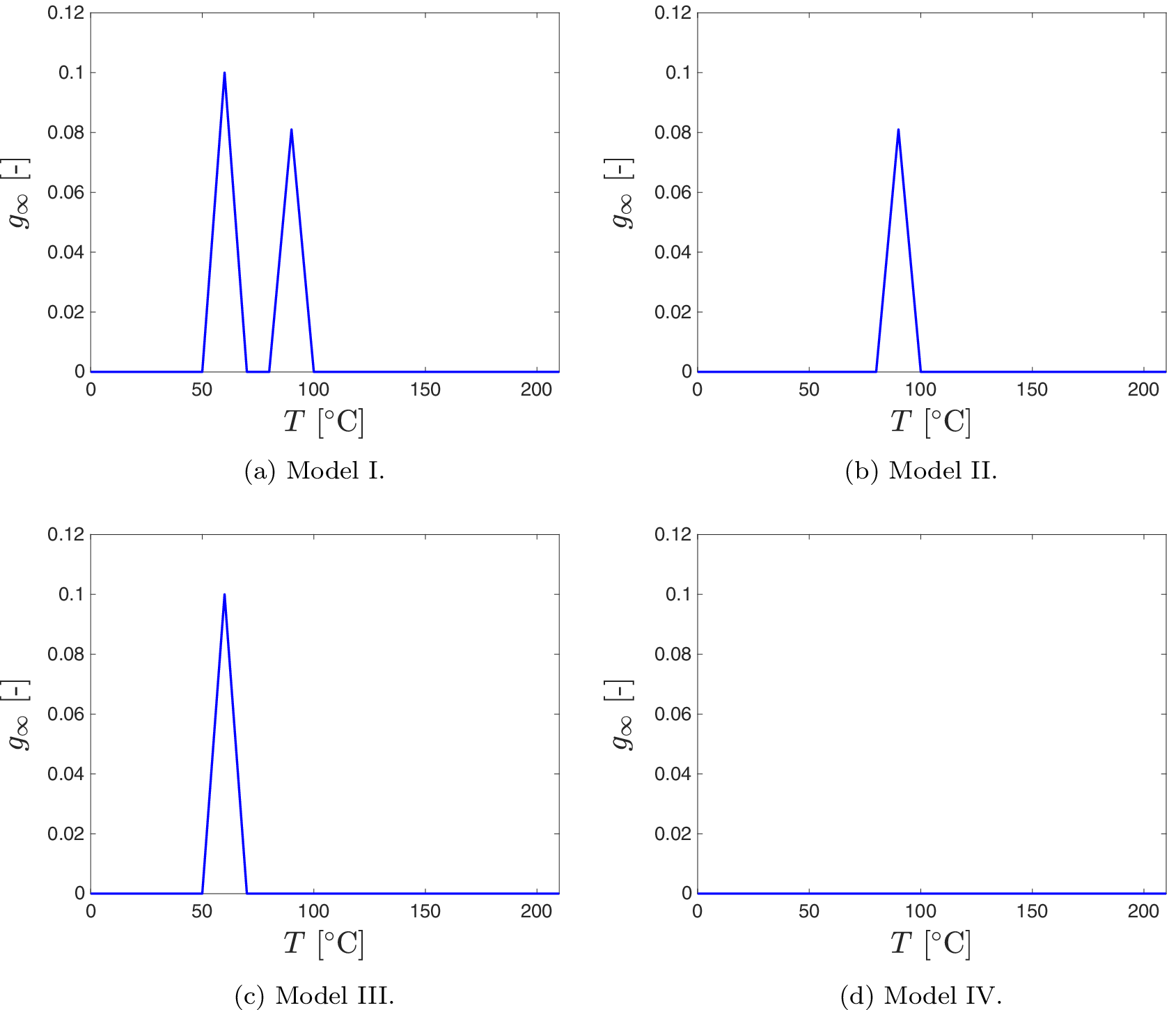
In model I (i.e., “Full aging model”), the growth of the fracture stress is incorporated for aging temperatures of 60 °C and 90 °C. The infinity growth function associated with this model is graphically presented in Figure 4a. Model II only allows growth to take place at an aging temperature of 90 °C. Its infinite growth function is presented in Figure 4b. Conversely, Model III enables growth of the fracture stress to take place at 60 °C and disallows fracture stress growth at 90 °C. The associated infinity growth function is presented in Figure 4c. Finally, Model IV does not allow any growth to take place. Hence, its infinity growth function is 0 everywhere.
Infinity growth functions
$ {g}_{\infty }(T) $
 of the four different aging models. The infinity growth function is the only difference between the four aging models.

Figure 4. Long description
The four panels share identical axes. The horizontal x-axis represents temperature T in degrees Celsius, ranging from 0 to 200. The vertical y-axis represents the infinity growth function g sub infinity, ranging from 0 to 0.12.
* Panel a, Model I, located at the top-left, shows two distinct triangular peaks. The first peak reaches a height of 0.1 at approximately 60 degrees Celsius. The second peak reaches a height of 0.08 at approximately 90 degrees Celsius. Outside these narrow peaks, the value is zero.
* Panel b, Model II, located at the top-right, shows a single triangular peak reaching a height of 0.08 at approximately 90 degrees Celsius. The rest of the function is zero.
* Panel c, Model III, located at the bottom-left, shows a single triangular peak reaching a height of 0.1 at approximately 60 degrees Celsius. The rest of the function is zero.
* Panel d, Model IV, located at the bottom-right, shows a flat line at zero across the entire temperature range from 0 to 200 degrees Celsius.
It may be clear that the infinity growth functions in Figure 4 may not be ideally suited to link the observed fracture stress data to any underlying chemical changes. However, the objective here is to determine whether fracture stress growth should be incorporated into any model, and these functions are well-suited for that purpose.
4. Model selection
In order to incorporate all the experimental data, model selection is applied to four aging models of the previous section. Two information criteria are exploited for model selection: the Akaike information criterion (AIC) (Akaike, Reference Akaike1974) and the Bayesian information criterion (BIC) (Schwarz, Reference Schwarz1978). For a model calibrated using least squares, they can be calculated as follows:


where
$ {n}_{\mathrm{p}} $
 denotes the number of model parameters,
$ {n}_{\mathrm{m}} $
 denotes the number of experimental observations, and the residual sum of squares is expressed as follows:

where
$ {\tilde{\sigma}}_{\mathrm{f}/i} $
 denotes a fracture stress measurement recorded for aging temperature
$ {T}_i $
 and aging duration
$ {t}_i $
 .
$ {\sigma}_{\mathrm{f}} $
 denotes the model response for the same aging temperature and aging duration.
Both information criteria consist of two contributions. The first contribution quantifies the “costs” of the model and uses the number of model parameters to do so (and the number of experimental observations in the case of the BIC). The second contribution quantifies the “gains” of the model (i.e., the accuracy), which is quantified identically in the two criteria. It may be clear that a model with a small AIC or BIC value is favored over those with larger values.
Because the absolute AIC and BIC values are affected by constants that are shared by all models, relative probabilities are generally considered instead of absolute values (Burnham and Anderson, Reference Burnham and Anderson2004). To provide the definition of these relative probabilities, the four models are again denoted by I, II, III, and IV. The minimal AIC and BIC values among these models are determined and denoted by
$ {\mathrm{AIC}}_{\mathrm{min}} $
 and
$ {\mathrm{BIC}}_{\mathrm{min}} $
 , respectively. The relative likelihood of model
$ i $
 , is then calculated as follows:

where
$ \mathrm{AIC} $
 may be replaced by
$ \mathrm{BIC} $
 if the BIC is of interest. Thus,
$ {p}_i $
 quantifies the relative probability that model
$ i $
 performs better than the other models. In AIC terminology,
$ {p}_i $
 are called the Akaike weights.
Finally, it may be observed that the original AIC (Akaike, Reference Akaike1974) is employed here and not the extension for a small number of data (Suguria, Reference Suguria1978). The reason is that the amount of gathered data is substantial relative to the number of model parameters. In such cases, the difference between the two AIC variants is insignificant (as was confirmed by the authors for this study’s data, but not reported).
5. Results
This section presents the results of the statistical hypothesis tests that are directly applied to the experimental data (Subsection 1), the calibration of the aging models (Subsection 2), and the results of the model selection (Subsection 3).
5.1. Model-free statistical hypothesis tests
Before discussing the results of the model-free statistical hypothesis tests, it is again iterated that the larger the p-value, the more probable the data in the two sets differ only due to random chance. Literature most commonly assumes that a p-value less than 0.05 or 0.01 indicates that the differences between the two datasets are caused by a statistically significant, underlying effect.
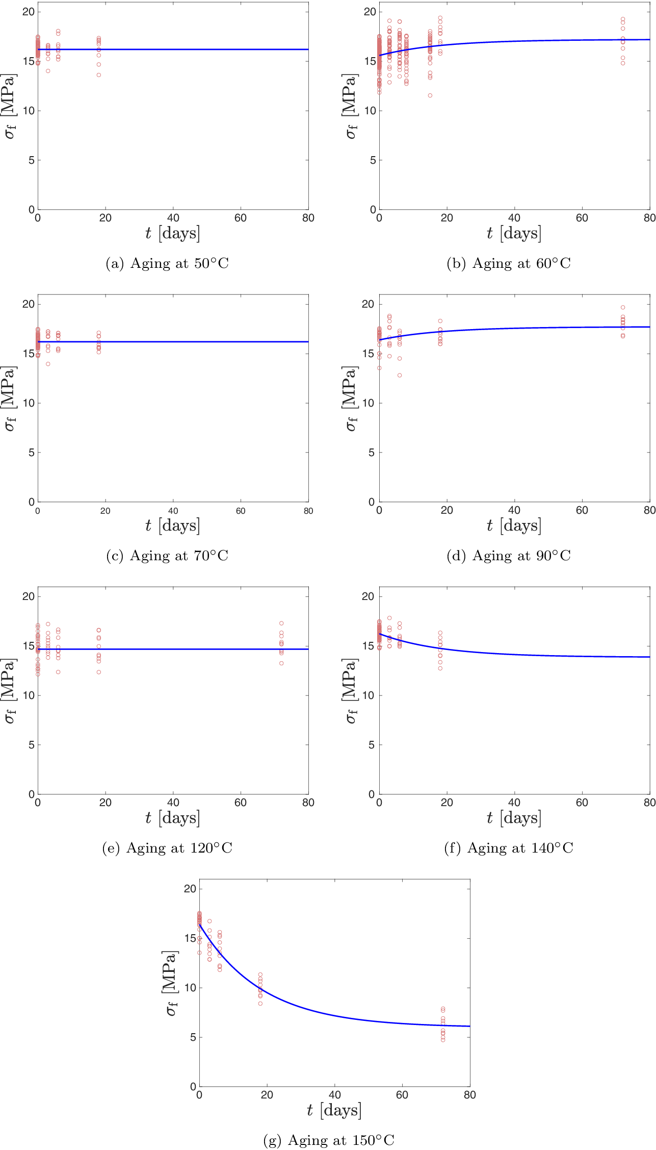
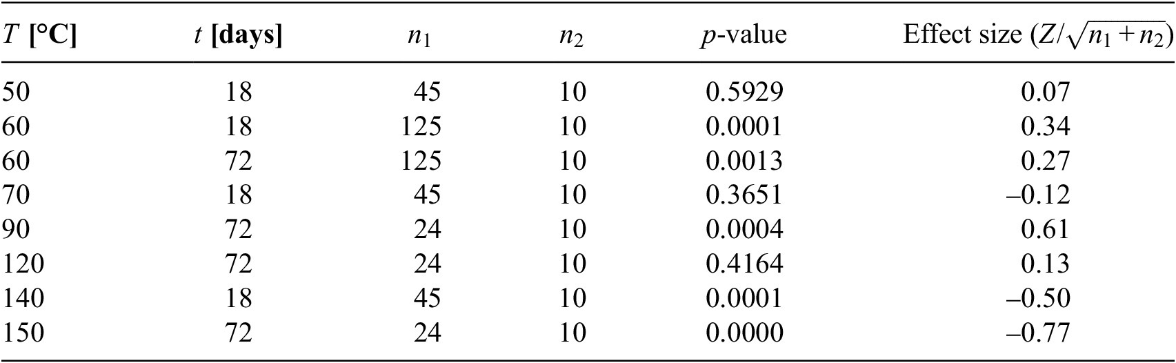
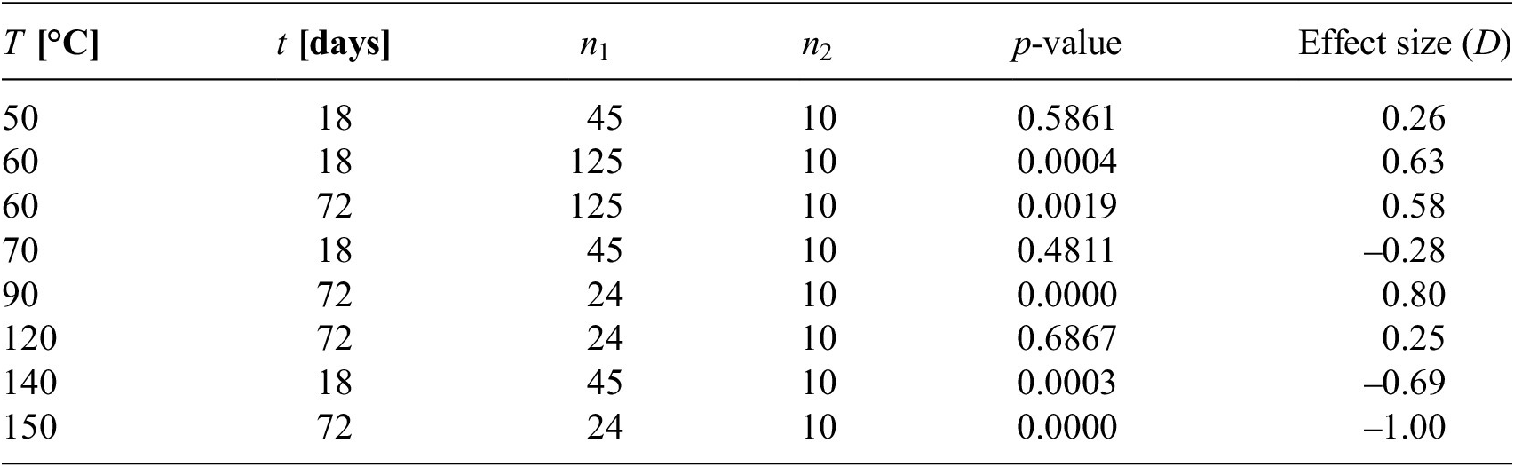
With that in mind, attention is directed to the experimentally recorded fracture stresses in Figure 5 and the results of the two-tailed MWU test and the two-sample KS test in Tables 1 and 2, respectively. The p-values of both tests are substantially greater than 0.05 and 0.01, or substantially lower. This means that there are no doubts about whether the null hypothesis (i.e., the differences between the datasets are caused by random chance alone) is accepted (large p-values) or rejected (small p-values).
Comparison of the fracture stress measurements (red circles) with the calibrated responses (blue lines) of aging Model I (which incorporates both degradation and growth).

Figure 5. Long description
A multi-panel figure containing seven line graphs labeled a through g. Each graph shares the same axes. The horizontal x-axis is t in days, ranging from 0 to 80. The vertical y-axis is sigma sub f in M P a, ranging from 0 to 20. Red circles represent individual measurements and a solid blue line represents the model response.
* Panel a, Aging at 50 degrees Celsius. The blue line is nearly horizontal at approximately 16 M P a.
* Panel b, Aging at 60 degrees Celsius. The blue line shows a slight asymptotic increase from 16 to 17.5 M P a.
* Panel c, Aging at 70 degrees Celsius. The blue line is horizontal at 16 M P a.
* Panel d, Aging at 90 degrees Celsius. The blue line shows a slight asymptotic increase from 16.5 to 18 M P a.
* Panel e, Aging at 120 degrees Celsius. The blue line is horizontal at approximately 15 M P a.
* Panel f, Aging at 140 degrees Celsius. The blue line shows an asymptotic decrease from 16 to 14 M P a.
* Panel g, Aging at 150 degrees Celsius. The blue line shows a significant asymptotic decrease from 17 M P a at day 0 to approximately 6 M P a at day 80. The red data points are more widely scattered in this panel compared to lower temperatures.
Two-tailed MWU test results

Table 1. Long description
The table consists of six columns and eight data rows. The columns are labeled as follows: T in degrees Celsius, t in days, n sub 1, n sub 2, p-value, and Effect size calculated as Z all over the square root of the sum of n sub 1 and n sub 2.
* Row 1: 50 degrees Celsius, 18 days, n sub 1 is 45, n sub 2 is 10, p-value is 0.5929, effect size is 0.07.
* Row 2: 60 degrees Celsius, 18 days, n sub 1 is 125, n sub 2 is 10, p-value is 0.0001, effect size is 0.34.
* Row 3: 60 degrees Celsius, 72 days, n sub 1 is 125, n sub 2 is 10, p-value is 0.0013, effect size is 0.27.
* Row 4: 70 degrees Celsius, 18 days, n sub 1 is 45, n sub 2 is 10, p-value is 0.3651, effect size is negative 0.12.
* Row 5: 90 degrees Celsius, 72 days, n sub 1 is 24, n sub 2 is 10, p-value is 0.0004, effect size is 0.61.
* Row 6: 120 degrees Celsius, 72 days, n sub 1 is 24, n sub 2 is 10, p-value is 0.4164, effect size is 0.13.
* Row 7: 140 degrees Celsius, 18 days, n sub 1 is 45, n sub 2 is 10, p-value is 0.0001, effect size is negative 0.50.
* Row 8: 150 degrees Celsius, 72 days, n sub 1 is 24, n sub 2 is 10, p-value is 0.0000, effect size is negative 0.77.
A note indicates that positive effect sizes show fracture stress growth, while negative signs indicate degradation over time.
Note: The sign of the effect size indicates whether the fracture stress grows (+) or degrades (-) over time.
Two-sample KS test results
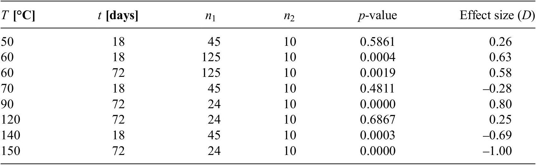
Table 2. Long description
The table consists of six columns and eight data rows.
Column headers are:
1. T degrees Celsius.
2. t days.
3. n sub 1.
4. n sub 2.
5. p-value.
6. Effect size D.
Data rows:
* Row 1: 50, 18, 45, 10, 0.5861, 0.26.
* Row 2: 60, 18, 125, 10, 0.0004, 0.63.
* Row 3: 60, 72, 125, 10, 0.0019, 0.58.
* Row 4: 70, 18, 45, 10, 0.4811, negative 0.28.
* Row 5: 90, 72, 24, 10, 0.0000, 0.80.
* Row 6: 120, 72, 24, 10, 0.6867, 0.25.
* Row 7: 140, 18, 45, 10, 0.0003, negative 0.69.
* Row 8: 150, 72, 24, 10, 0.0000, negative 1.00.
A note below the table states that the sign of the effect size indicates whether the fracture stress grows plus or degrades minus over time.
Note: The sign of the effect size indicates whether the fracture stress grows (+) or degrades (-) over time.
Another observation from Tables 1 and 2, which reinforces the belief in the p-values, is that the MWU and KS tests produce highly similar p-values across all examined combinations of datasets.
The p-values clearly indicate that the fracture stresses associated with aging at 50 °C, 70 °C, and 120 °C are not different from the fracture stresses of unaged rubber. Thus, the fracture stress does not evolve over time for these aging temperatures. Tables 1 and 2 also show that the effect sizes for these three aging temperatures are small. This is expected if the datasets lack statistical significance.
The p-values for the other aging temperatures of 60 °C, 90 °C, 140 °C, and 150 °C are substantially lower than 0.05 and even substantially lower than 0.01. Consequently, it is easy to argue that statistical significance is associated with these aging temperatures. In other words, both statistical hypothesis tests indicate a high probability that the fracture stress evolves over time for these aging temperatures.
To quantify the magnitude of the evolution of the fracture stress for these aging temperatures, the effect sizes must be considered. For aging temperatures of 60 °C and 90 °C, both the MWU and KS tests indicate that the fracture stress grows, whereas for 140 °C and 150 °C, both tests indicate a degradation of the fracture stress. The effect sizes calculated by the two tests are not the same. However, this can be explained by the fact that they use different test statistics: the MWU test focuses on central location (via ranking), whereas the KS test investigates both central location and shape (via the maximum vertical difference between the two eCDFs). However, the relative ratios of the effect sizes match satisfactorily.
In summary, both hypothesis tests indicate without doubt that the fracture stress degrades for aging at 140 °C and 150 °C, remains the same for aging at 50 °C, 70 °C, and 120 °C, and grows for aging at 60 °C and 90 °C. On the other hand, the tests do not incorporate all experimental data.
5.2. Calibrated model responses
The current subsection presents the calibration of the aging model of Section 3. It focuses on Model I’s calibration results (full aging model), because the other three models are obtained by setting some values of infinity growth function
$ {g}_{\infty }(T) $
 to 0.
The parameters of the aging models are reference fracture stress
$ {\sigma}_{\mathrm{f}}^{\mathrm{ref}} $
 , time-scale parameter
$ \tau $
 , and the parameters that describe infinity degradation function
$ {d}_{\infty }(T) $
 and infinity growth function
$ {g}_{\infty }(T) $
 . The data for aging at 150 °C in Figure 5(g) show the neatest temporal trend. Therefore, these data are used to calibrate
$ {\sigma}_{\mathrm{f}}^{\mathrm{ref}} $
 ,
$ \tau $
 , and
$ {d}_{\infty}\Big(T=150{}^{\circ} $
 C
$ \Big) $
 simultaneously, while
$ {g}_{\infty}\Big(T=150{}^{\circ} $
 C
$ \Big)=0 $
 to prevent indeterminacy. With
$ {\sigma}_{\mathrm{f}}^{\mathrm{ref}} $
 and
$ \tau $
 now calibrated, the data for aging at 140 °C are used to calibrate
$ {d}_{\infty}\Big(T=140{}^{\circ} $
 C
$ \Big) $
 , while
$ {g}_{\infty}\Big(T=140{}^{\circ} $
 C
$ \Big)=0 $
 to prevent indeterminacy. The values of
$ {d}_{\infty } $
 at all the other aging temperatures tested are set to 0, because no degradation occurs (
$ 50{}^{\circ} $
 C,
$ 70{}^{\circ} $
 C, and
$ 100{}^{\circ} $
 C) or to prevent indeterminacy in the identification of
$ {g}_{\infty}\Big(T=60{}^{\circ} $
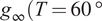 C
$ \Big) $
 and
$ {g}_{\infty}\Big(T=90{}^{\circ} $
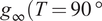 C
$ \Big) $
 .
All values of
$ {g}_{\infty } $
 are set to zero, except for aging at 60 °C and for aging at 90 °C. For these two aging temperatures, the identification of
$ {g}_{\infty}\Big(T=60{}^{\circ} $
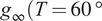 C
$ \Big) $
 and
$ {g}_{\infty}\Big(T=90{}^{\circ} $
 C
$ \Big) $
 is straightforward since
$ {\sigma}_{\mathrm{f}}^{\mathrm{ref}} $
 and
$ \tau $
 have already been calibrated using the response for 150 °C.
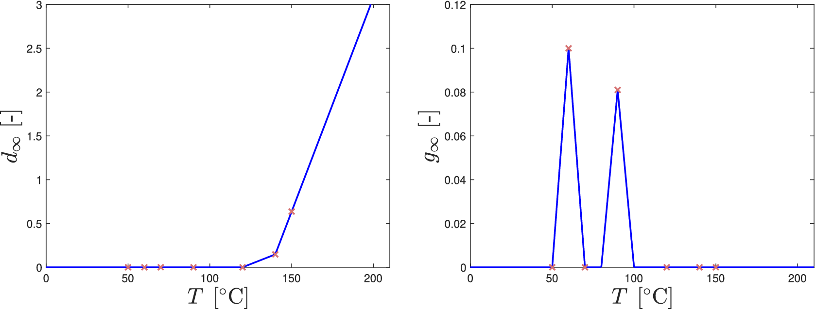
The resulting infinity degradation function
$ {d}_{\infty }(T) $
 and infinity growth function
$ {g}_{\infty }(T) $
 are presented in Figure 6. Here, it is clear that piecewise linear functions are chosen for both expressions. The associated model responses in Figure 5 seem sufficiently accurate to the naked eye and yield a mean squared error of 1.5 MPa
$ {}^2 $
 upon closer inspection.
Infinity degradation function
$ {d}_{\infty }(T) $
 (left, blue line) and infinity degradation function
$ {g}_{\infty }(T) $
 (right, blue lines) for aging Model I (that incorporates both degradation and growth). The red crosses are data points obtained from the experimental data in Figure 5.

Figure 6. Long description
Two side-by-side line graphs.
Left Graph:
* The x-axis is labeled T in degrees Celsius, ranging from 0 to 200.
* The y-axis is labeled d sub infinity, ranging from 0 to 3.
* The data is represented by a blue line with red crosses as data points.
* The line remains at 0 until approximately 120 degrees Celsius. It then shows a sharp linear increase, passing through data points at 140 degrees Celsius (y is approximately 0.2) and 150 degrees Celsius (y is approximately 0.6), continuing upward to y equals 3 at 200 degrees Celsius.
Right Graph:
* The x-axis is labeled T in degrees Celsius, ranging from 0 to 200.
* The y-axis is labeled g sub infinity, ranging from 0 to 0.12.
* The data is represented by blue lines forming two distinct triangular peaks.
* The first peak starts at 50 degrees Celsius, reaches a maximum of 0.1 at 60 degrees Celsius, and returns to 0 at 70 degrees Celsius.
* The second peak starts at 80 degrees Celsius, reaches a maximum of approximately 0.08 at 90 degrees Celsius, and returns to 0 at 100 degrees Celsius.
* Red crosses mark the base and peak of these triangles, as well as several points at y equals 0 between 120 and 150 degrees Celsius.
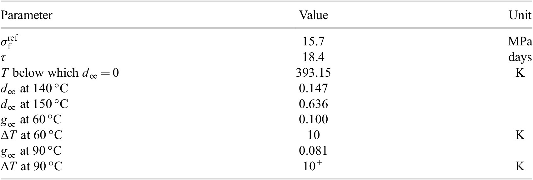
The calibrated parameter values of this aging model (i.e., the full aging model, which incorporates both degradation and growth) are presented in Table 3. It is repeated again that Model II is obtained by forcing
$ {g}_{\infty}\Big(T=60{}^{\circ} $
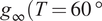 C
$ \Big)=0 $
 , Model III by forcing
$ {g}_{\infty}\Big(T=90{}^{\circ} $
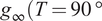 C
$ \Big)=0 $
 , and Model IV by forcing
$ {g}_{\infty}\Big(T=60{}^{\circ} $
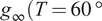 C
$ \left)={g}_{\infty}\right(T=90{}^{\circ} $
 C
$ \Big)=0 $
 , as previously presented in Figure 4.
Calibrated parameter values for aging Model I (which incorporates both degradation and growth)

Table 3. Long description
The table consists of three columns: Parameter, Value, and Unit.
* Row 1: sigma sub f super ref, 15.7, M P a.
* Row 2: tau, 18.4, days.
* Row 3: T below which d sub infinity equals 0, 393.15, K.
* Row 4: d sub infinity at 140 degrees C, 0.147, (no unit).
* Row 5: d sub infinity at 150 degrees C, 0.636, (no unit).
* Row 6: g sub infinity at 60 degrees C, 0.100, (no unit).
* Row 7: Delta T at 60 degrees C, 10, K.
* Row 8: g sub infinity at 90 degrees C, 0.081, (no unit).
* Row 9: Delta T at 90 degrees C, 10 black square, K.
A footnote indicates that the black square symbol signifies the value was chosen.
Note: Symbol
$ {}^{+} $
 indicates that the value is chosen.
5.3. Model selection
Finally, the results of the model selection are discussed. The fracture stress data for unaged rubber (i.e., at
$ t=0 $
 ) are ignored in the analyses of Table 4, because their number is substantially larger than for the other aging durations, and they are only needed to calibrate the reference fracture stress
$ {\sigma}_{\mathrm{f}}^{\mathrm{ref}} $
 . If they were incorporated, the relative BIC results (
$ {p}^{\mathrm{BIC}} $
 ) would be similar to the relative AIC results (
$ {p}^{\mathrm{AIC}} $
 ), while the relative AIC results would hardly change. This is confirmed by the authors, but not reported.
Model selection results

Table 4. Long description
The table consists of seven columns and five rows including the header.
Columns from left to right are: Model Name, n sub p, R S S, A I C, B I C, p super A I C, and p super B I C.
Row 1 (Header): Model Name, n sub p, R S S, A I C, B I C, p super A I C, p super B I C.
Row 2 (I: full aging model): n sub p is 9, R S S is 565.4, A I C is 170.8, B I C is 206.2, p super A I C is 0.99, p super B I C is 0.58.
Row 3 (II: without growth at 60 degrees Celsius): n sub p is 7, R S S is 667.6, A I C is 229.5, B I C is 257.0, p super A I C is 0.00, p super B I C is 0.00.
Row 4 (III: without growth at 90 degrees Celsius): n sub p is 7, R S S is 584.5, A I C is 179.3, B I C is 206.8, p super A I C is 0.01, p super B I C is 0.42.
Row 5 (IV: without growth where g sub infinity of T equals 0): n sub p is 5, R S S is 686.8, A I C is 236.3, B I C is 255.8, p super A I C is 0.00, p super B I C is 0.00.
A footnote indicates that n sub m equals 377 for all models.
Note:
$ {n}_{\mathrm{m}}=377 $
 is the same for all models.
The relative AIC results in Table 4 leave no doubt that the full aging model (Model I) outperforms all other aging models. The second-best aging model is the model that only considers growth at 60 °C and ignores growth at 90 °C, and only has a relative likelihood of 0.01 versus a relative likelihood of 0.99 for the full aging model. (This does not imply that fracture stress growth at 60 °C is ‘more physical’ than the growth at 90 °C. It only means that the growth at 60 °C is more important to incorporate in an aging model than the growth at 90 °C.)
The BIC results in Table 4 indicate a greater relative likelihood for the aging model that only considers growth at 60 °C and ignores growth at 90 °C than the AIC results. Yet, according to the BIC, the full aging model is the most suited aging model with a relative likelihood of 0.58.
Thus, the AIC and BIC model selection results indicate that growth at 60 °C is more important to incorporate than growth at 90 °C, whereas the statistical hypothesis tests of the data have indicated that the fracture stress grows more for aging at 90 °C than at 60 °C. On the one hand, the model selection results may seem more trustworthy because they consider all experimental data. On the other hand, model-free statistical hypothesis tests do not involve modeling assumptions of the aging model. Regardless, both types of results indicate that the fracture stress of the peroxide-cured EPDM rubber of interest not only degrades due to thermal oxidative aging, but also grows for some aging temperatures—as was also observed in (Ning et al. (Reference Ning, Ma, Zhang, Zhang, Wu and Tian2014), Öncel et al. (Reference Öncel, Gül, Efe, Erdoğan and Karaağaç2023).
6. Summary and conclusion
This study has demonstrated the application of statistical hypothesis tests of experimental data and model selection as means to investigate trends in scattered aging data. Statistical hypothesis tests of data have the advantage that their results are unaffected by modeling choices. However, they are unable to consider all experimental data if the data evolve over time. On the other hand, model selection considers all experimental data, but comes with the disadvantages that (i) only proposed models are investigated against the data, and (ii) it is associated with modeling assumptions, since all models come with modeling choices.
Here, it is relevant to mention that the model selection approaches of this study are only applicable if the models are deterministically calibrated using least-squares minimization. Consequently, the approaches do not, strictly speaking, constitute true hypothesis tests. In contrast, model selection based on the Bayes factor represents a genuine statistical hypothesis testing framework. The reason to focus on model selection for deterministic identification is nevertheless justified by the fact that deterministic identification is better understood by a large part of the community than probabilistic identification. This makes the exploited model selection approaches readily accessible to practitioners who may not be familiar with probabilistic methods such as Bayesian inference. Moreover, probabilistic identification not only requires specialized sampling algorithms, but the computation of Bayes factors also depends on dedicated methods for estimating the marginal likelihood (e.g., bridge sampling or thermodynamic integration).
Model-free statistical hypothesis tests and model selection are used to quantitatively investigate whether the fracture stress of the peroxide-cured EPDM rubber of interest exhibits improvement due to short-term thermal oxidative aging for certain aging temperatures. This in-depth investigation is performed because fracture stress improvement goes against the general consensus that the fracture stress only degrades due to thermal oxidative aging, and because the experimental data exhibit substantial scatter.
The statistical hypothesis tests directly applied to the experimental data are the two-tailed Wilcoxon-Mann–Whitney U (MWU) test and the two-sample Smirnov test, which is better known as the two-sample Kolmogorov–Smirnov (KS) test. Although the two tests focus on different metrics, their p-values are highly similar. On top of that, the p-values are far below and above the widely used critical values of 0.01 and 0.05. This means that the results of the two tests leave no doubt about statistical significance: the fracture stress improves for aging temperatures of 60 °C and 90 °C due to thermal oxidative aging (for short aging durations).
Besides the p-values, the effect size was also investigated. For the fracture stress data investigated here, the effect size indicates how much the fracture stress improves or degrades for certain aging temperatures. The calculated effect sizes differ more than the p-values due to the use of different test statistics. However, relative to each other, the effect sizes calculated by the MWU test and the KS test are similar.
Model selection was applied in order to consider all experimental data—which is impossible in the hypothesis tests of the data. Model selection can be considered stricter than the aforementioned statistical hypothesis tests, because model selection quantitatively assesses model complexity versus model accuracy. This means that even if Model A is more accurate than Model B, Model B can still be preferred if it is less complex than Model A.
Model selection was applied to four different aging models. All models incorporated fracture stress degradation, but differed in the way they incorporated fracture stress improvement. Model selection was applied via the Akaike information criterion (AIC) and the Bayesian information criterion (BIC). The BIC favors model simplicity more strongly than the AIC.
The results of both the AIC and the BIC indicate that the aging model that fully incorporates fracture stress improvement is the most suited. This confirms the results of the model-free statistical hypothesis tests that the fracture stress indeed grows for certain aging temperatures. A minor difference between the two types of tests is that the model selection results indicate that fracture stress improvement for aging at 60 °C is more important than the improvement at 90 °C, whereas the results of the statistical hypothesis tests of the data indicate the opposite.
Although this study has only applied the two methods to one material property (fracture stress) affected by one physical phenomenon (thermal oxidative aging), the two methods can be applied to any material property affected by any physical phenomenon. Hence, the evolution of the fracture stress due to thermal aging was only a demonstrative example: the methods can also be used to study crack length due to ozone attack, the modulus due to thermal aging, and the fracture stress due to ultraviolet irradiation, to name a few examples.
Data availability statement
The industrial partner has asked the authors not to share any raw experimental data. The compound of the investigated EPDM compound is protected by intellectual property and is unknown to the authors. The authors only know that the EPDM contains an anti-degradant.
Acknowledgments
The authors, and in particular Aravind Kadhambariyil, would like to acknowledge (late) Thomas Dieckmann, Andreas Brueck, Andreas Schaal, and Bernd Hackenberger of SISTO Armaturen SA for their support with the experimental campaign. The authors are also grateful for the financial support of SISTO Armaturen SA.
Author contribution
Conceptualization: L.B., Data curation: A.K., Formal analysis: L.B., Funding acquisition: S.B., L.B., Investigation: A.K., Methodology: A.K., L.B., Project administration: S.B., L.B., Resources: A.K., Software: A.K., Supervision: S.B., L.B., Validation: A.K., Visualization: A.K., Writing – original draft: A.K., L.B., Writing – review and editing: S.B., L.B.
Funding statement
Aravind Kadhambariyil’s PhD studies are financed by SISTO Armaturen SA.
Competing interests
Although Aravind Kadhambariyil’s PhD studies are financed by SISTO Armaturen SA, he is not an employee of SISTO Armaturen SA but of the University of Luxembourg. SISTO Armature SA has not influenced the methodology or results of this study, nor is it expected to capitalize on this study’s outcomes—to the best of the authors’ understanding.







 Open access


Comments
No Comments have been published for this article.