2 Simulation configuration and discretization

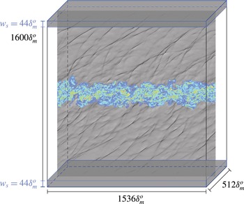
The compressible flow equations, formulated in Cartesian coordinates, were solved for the temporally developing shear layer shown in figure 1. The simulation domain extends $L_{x}\times L_{y}\times L_{z}=1536\unicode[STIX]{x1D6FF}_{m}^{o}\times 1600\unicode[STIX]{x1D6FF}_{m}^{o}\times 512\unicode[STIX]{x1D6FF}_{m}^{o}$ in the streamwise $x$ , cross-stream $y$ and spanwise $z$ directions, respectively, with $\unicode[STIX]{x1D6FF}_{m}^{o}=\unicode[STIX]{x1D6FF}_{m}(0)$ the initial momentum thickness. The momentum thickness at time $t$ is

(2.1) $$\begin{eqnarray}\unicode[STIX]{x1D6FF}_{m}(t)=\frac{1}{\unicode[STIX]{x1D70C}_{\infty }\unicode[STIX]{x0394}U^{2}}\int _{-L_{y}/2}^{L_{y}/2}\bar{\unicode[STIX]{x1D70C}}\left[\frac{1}{2}\unicode[STIX]{x0394}U-\tilde{u} (y,t)\right]\left[\frac{1}{2}\unicode[STIX]{x0394}U+\tilde{u} (y,t)\right]\text{d}y,\end{eqnarray}$$

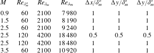
where $\unicode[STIX]{x0394}U$ is the velocity difference across the shear layer and $\tilde{u} (y,t)$ is the Favre-averaged mean flow. For most of the simulations, which are summarized in table 1, the Reynolds number based on the momentum thickness,

(2.2) $$\begin{eqnarray}Re_{\unicode[STIX]{x1D6FF}_{m}}=\frac{\unicode[STIX]{x1D70C}_{\infty }\unicode[STIX]{x0394}U\unicode[STIX]{x1D6FF}_{m}(t)}{\unicode[STIX]{x1D707}},\end{eqnarray}$$

increases from $Re_{\unicode[STIX]{x1D6FF}_{m}}=60$ to $2100$ such that $\unicode[STIX]{x1D6FF}_{m}(t)/\unicode[STIX]{x1D6FF}_{m}^{o}=35$ at the final time. A supplementary $M=2.5$ flow with $Re_{\unicode[STIX]{x1D6FF}_{m}^{o}}=120$ was simulated until $Re_{\unicode[STIX]{x1D6FF}_{m}}=4200$ to confirm Reynolds number insensitivity. The initial condition included the turbulence velocity perturbations of Kleinman & Freund (Reference Kleinman and Freund2008) to a streamwise velocity profile

(2.3) $$\begin{eqnarray}\bar{u}(y)=\frac{\unicode[STIX]{x0394}U}{2}\tanh \left(\frac{y}{2\unicode[STIX]{x1D6FF}_{m}^{o}}\right).\end{eqnarray}$$

The free-stream temperatures and sound speeds ( $c_{\infty }$ ) were identical and four flow speeds were simulated: $M=\unicode[STIX]{x1D6E5}U/c_{\infty }=0.9$ , $1.5$ , $2.5$ and $3.5$ .

Figure 1.

Simulation domain schematic. The shaded regions represent the extent of the sponge in (2.5).

Table 1.

Simulation parameters. The final Reynolds number for $Re_{\unicode[STIX]{x1D6FF}_{m}}$ and $Re_{\unicode[STIX]{x1D6FF}_{99}}$ correspond to $\unicode[STIX]{x1D6FF}_{m}(t)/\unicode[STIX]{x1D6FF}_{m}^{o}=35$ .

The simulation domain visualized in figure 1 was discretized with $N_{x}\times N_{y}\times N_{z}=1536\times 1601\times 512$ uniformly distributed mesh points with spacing $\unicode[STIX]{x1D6E5}=\unicode[STIX]{x1D6FF}_{m}^{o}$ . The resolution was doubled ( $\unicode[STIX]{x1D6E5}=1/2\unicode[STIX]{x1D6FF}_{m}^{o}$ ) for the $Re_{\unicode[STIX]{x1D6FF}_{m}^{o}}=120$ case. Domain interior derivatives were computed with fourth-order, 13-point, resolution-optimized finite differences (Bogey & Bailly Reference Bogey and Bailly2004). Grid points adjacent the $y=\pm L_{y}/2$ boundaries used reduced-order centred then one-sided differences (Buchta Reference Buchta2016), although these are not expected to degrade the solution since they are far from the turbulence and inside absorbing sponge zones. The second derivatives and mixed derivatives for the viscous terms are approximated by repeated finite-difference approximations to first-derivative operators.

A combination of an absorbing sponge (Freund Reference Freund1997) augmented with one-dimensional characteristic radiation boundary conditions (Thompson Reference Thompson1987) was used to model an infinite extent in $y$ with a local radiation-like approximation. The sponge regions had width $w_{s}=44\,\unicode[STIX]{x1D6FF}_{m}^{o}$ within which a damping term was added to the governing equations ${\mathcal{N}}(\boldsymbol{q})=0$ such that

(2.4) $$\begin{eqnarray}{\mathcal{N}}(\boldsymbol{q})=-\unicode[STIX]{x1D709}(y)[\boldsymbol{q}-\boldsymbol{q}_{target}(y)],\end{eqnarray}$$

where $\boldsymbol{q}_{target}$ is the uniform condition of either free stream. The sponge strength increased quadratically toward $y=\pm L_{y}/2$ as

(2.5) $$\begin{eqnarray}\unicode[STIX]{x1D709}(y)=\left\{\begin{array}{@{}ll@{}}{\displaystyle \frac{1}{2}}\left[{\displaystyle \frac{|y|-\left({\displaystyle \frac{L_{y}}{2}}-w_{s}\right)}{w_{s}}}\right]^{2},\quad & |y|>{\displaystyle \frac{L_{y}}{2}}-w_{s}\\ 0,\quad & \text{otherwise}.\end{array}\right.\end{eqnarray}$$

Repeated applications of first-derivative finite-difference approximations can reduce computational cost, but for symmetric stencils this approach is well understood not to provide the realistic viscous dissipation of the highest-wavenumber disturbances supported by the mesh. To counter the mild instability that can result from its lack, a weak high-wavenumber numerical filtering was applied in all three coordinate directions, as is often done (Kleinman & Freund Reference Kleinman and Freund2008). A 13-point, fourth-order filter (Bogey & Bailly Reference Bogey and Bailly2004) was applied every numerical time step to each conservative variable. One filter application reduces the wavenumber $k_{c}\unicode[STIX]{x0394}=1.81$ component by $1$ per cent while completely damping the highest wavenumber $k\unicode[STIX]{x0394}=\unicode[STIX]{x03C0}$ . The effect of this filter on key observables is shown to be negligible in the Appendix.

Reported statistical quantities are averaged over all mesh points in the $x$ - and $z$ -directions. They are also averaged in time intervals of $\unicode[STIX]{x0394}t=20\unicode[STIX]{x1D6FF}_{m}^{o}/\unicode[STIX]{x0394}U$ (every $100\,\unicode[STIX]{x0394}t$ time steps) using a self-similarity scaling in $y$ as the shear layer spreads from $\unicode[STIX]{x1D6FF}_{m}(t)/\unicode[STIX]{x1D6FF}_{m}^{o}=15$ to $35$ (see § 3). The $\pm y$ symmetry is likewise exploited for averaging.

3 Shear-layer development

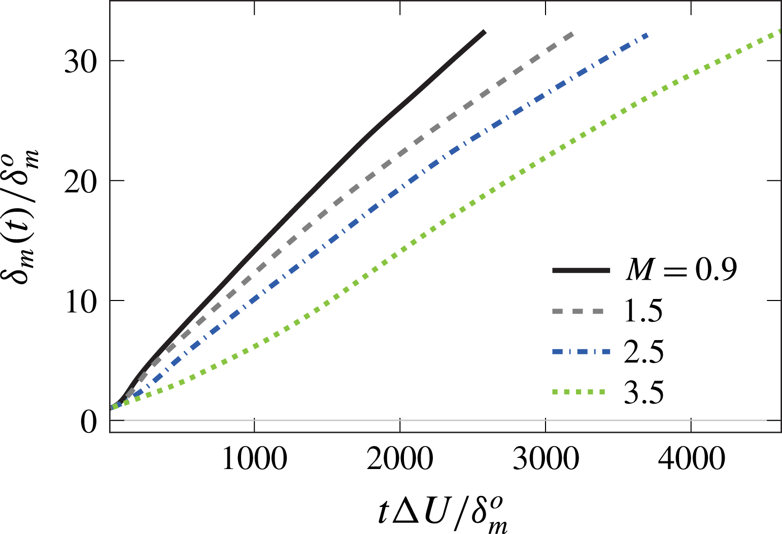
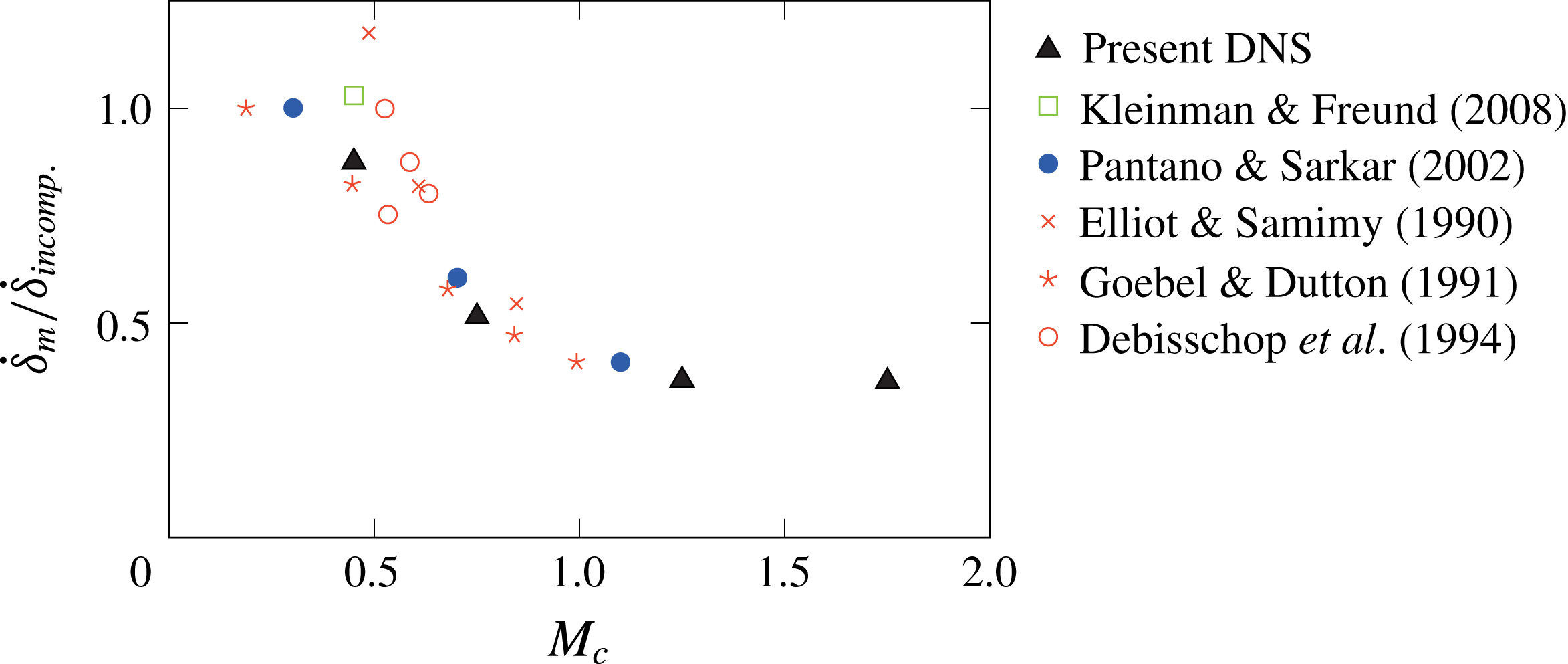
The growth of the turbulent shear layers is shown in figure 2. In all cases, after spreading by a factor of approximately 5, the growth is approximately linear between $15<\unicode[STIX]{x1D6FF}_{m}(t)/\unicode[STIX]{x1D6FF}_{m}^{o}<35$ , consistent with other simulations of this kind (Pantano & Sarkar Reference Pantano and Sarkar2002; Kleinman & Freund Reference Kleinman and Freund2008). Figure 3 shows that the growth rate of the simulations normalized by that expected for a corresponding incompressible fluid. As expected, based on previous observations, growth rate decreases with increasing

(3.1) $$\begin{eqnarray}M_{c}={\displaystyle \frac{\unicode[STIX]{x0394}U}{c_{\infty }+c_{j}}},\end{eqnarray}$$

and the trends with $M_{c}$ compare well with observations from spatially developing shear flows (Elliott & Samimy Reference Elliott and Samimy1990; Goebel & Dutton Reference Goebel and Dutton1991; Debisschop, Chambres & Bonnet Reference Debisschop, Chambres and Bonnet1994) and simulations of other temporally developing mixing layers (Pantano & Sarkar Reference Pantano and Sarkar2002; Kleinman & Freund Reference Kleinman and Freund2008).

Figure 2.

Shear-layer growth.

Figure 3.

Growth-rate suppression with $M_{c}$ (3.1). The nominal incompressible fluid growth rate $\dot{\unicode[STIX]{x1D6FF}}_{incomp.}=0.016$ is from the $M_{c}=0.3$ simulation of Pantano & Sarkar (Reference Pantano and Sarkar2002).

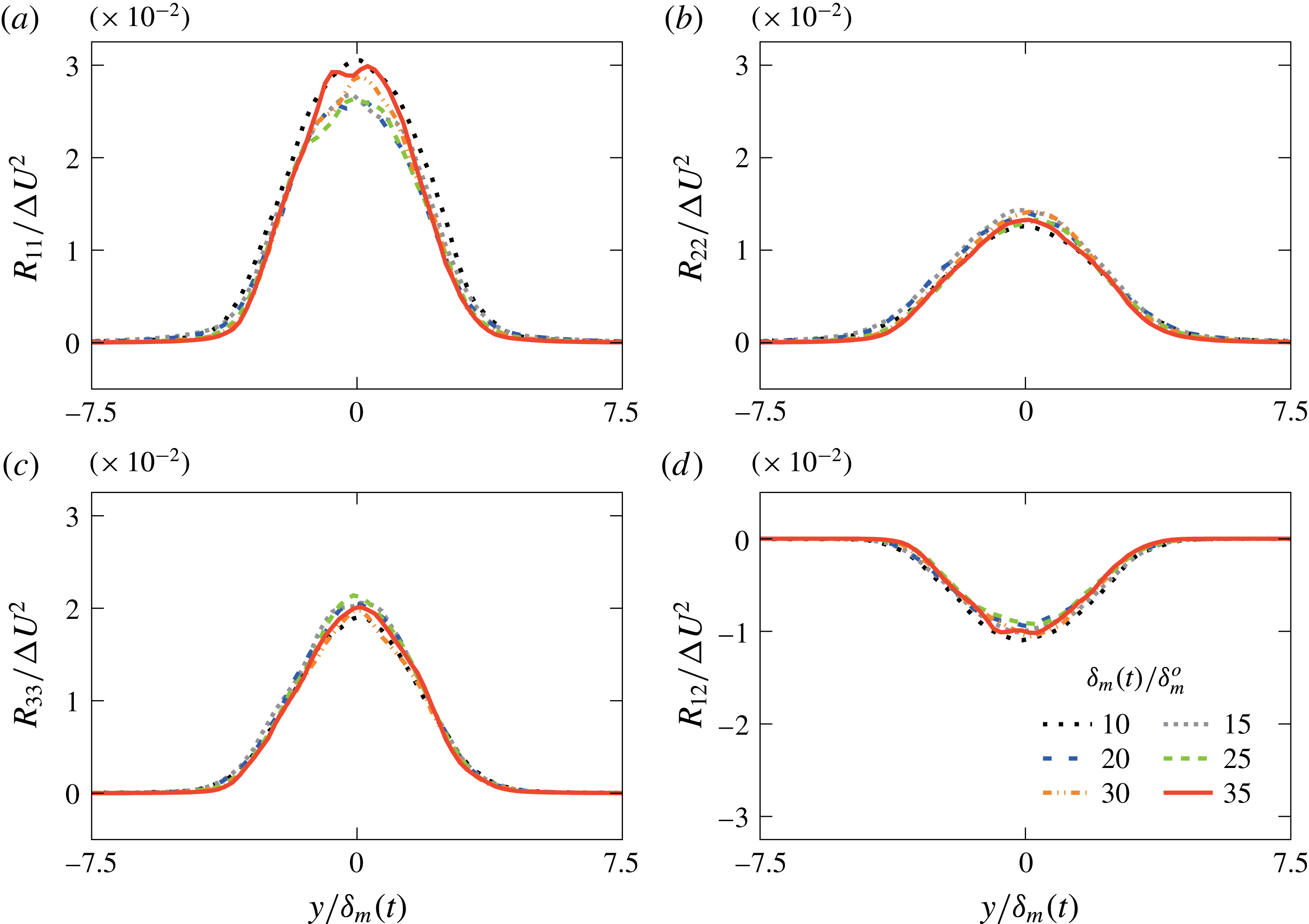
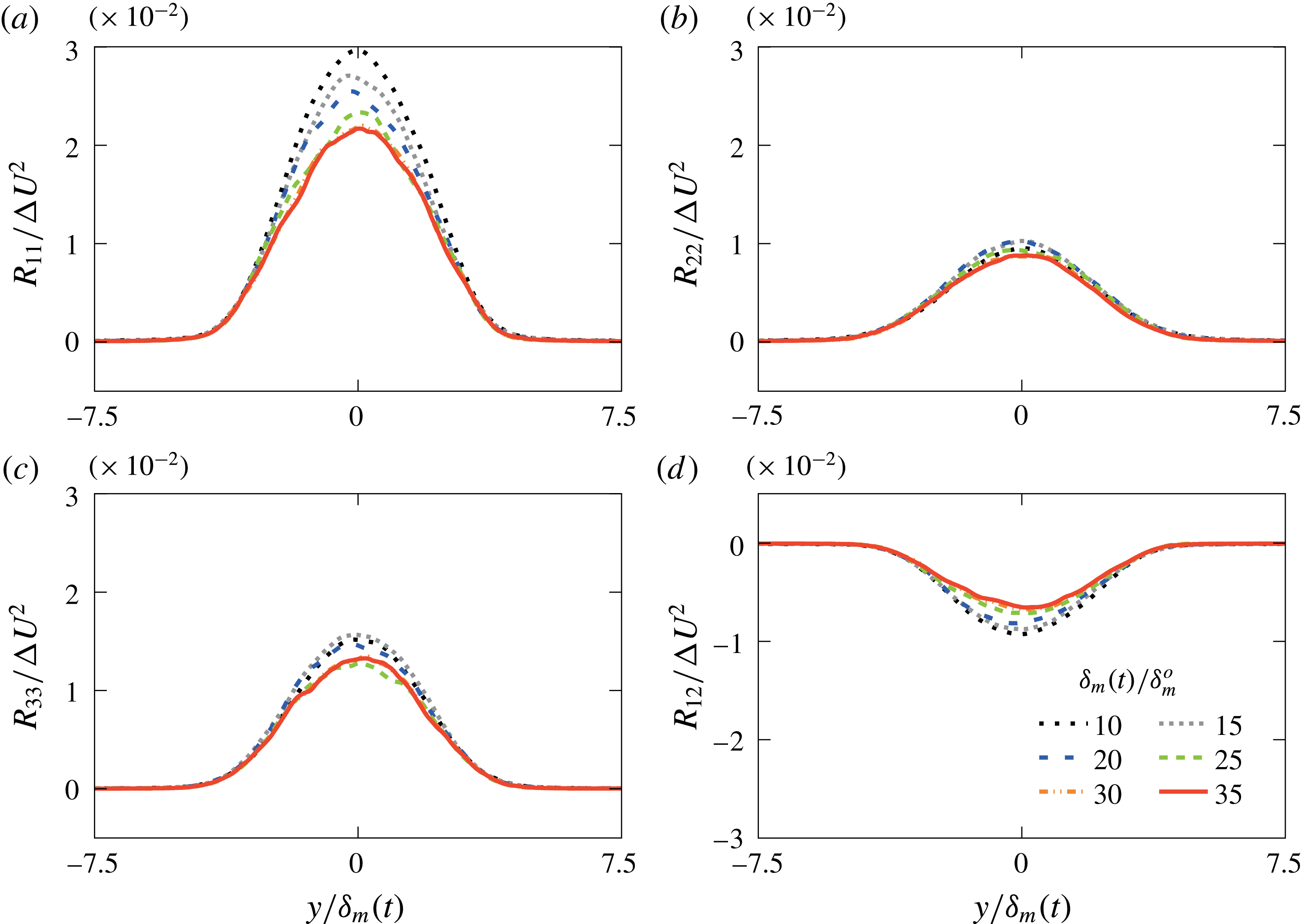
In a self-similar temporally developing flow, statistics should depend only on $y/\unicode[STIX]{x1D6FF}_{m}(t)$ , which does approximately collapse the Reynolds stresses in all cases. For $M=0.9$ in figure 4, the similarity scaling is particularly effective between $\unicode[STIX]{x1D6FF}_{m}(t)/\unicode[STIX]{x1D6FF}_{m}^{o}=10$ to $30$ . This collapse is slower to achieve, and ultimately not quite so complete for $M\geqslant 1.5$ , such as for the $M=2.5$ case shown in figure 5, although still sufficient for our averaging. A slower approach to self-similarity is expected based on experiments Elliott & Samimy (Reference Elliott and Samimy1990) and simulations (Pantano & Sarkar Reference Pantano and Sarkar2002). Similar statistics for all cases are reported in full detail elsewhere (Buchta Reference Buchta2016).

Figure 4.

Reynolds stress profiles for $M=0.9$ with shear-layer growth.

Figure 5.

Reynolds stress profiles for $M=2.5$ with shear-layer growth. Data from two additional ensembles with different initial random seeds are used for these statistics.

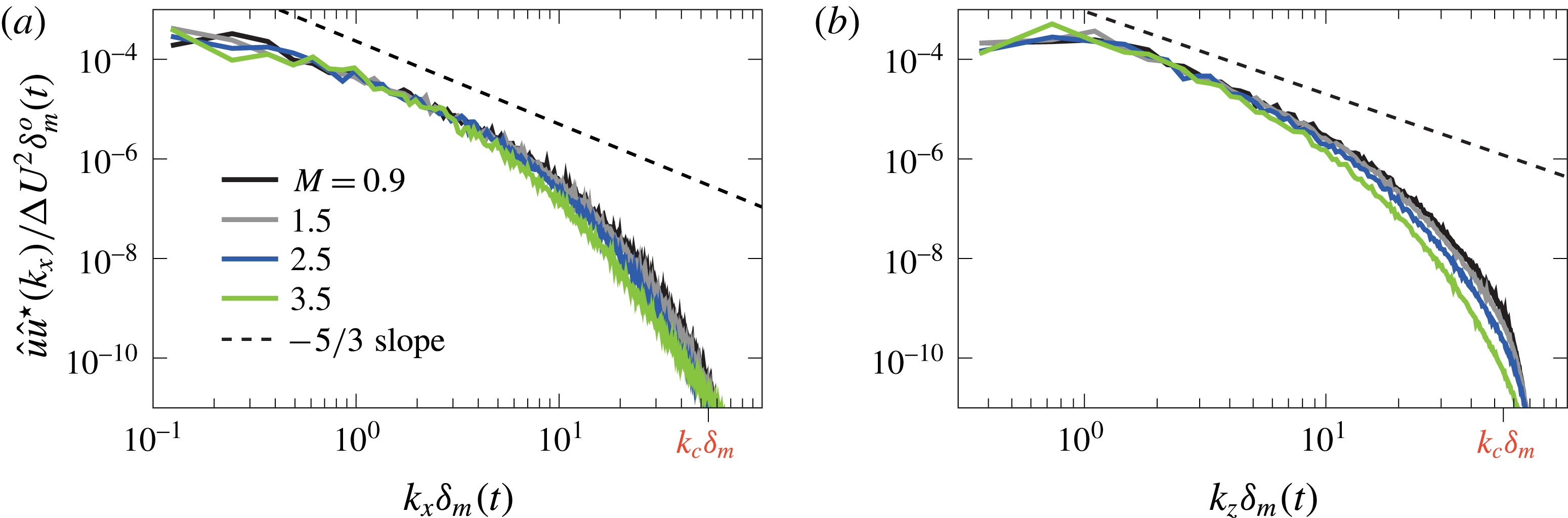
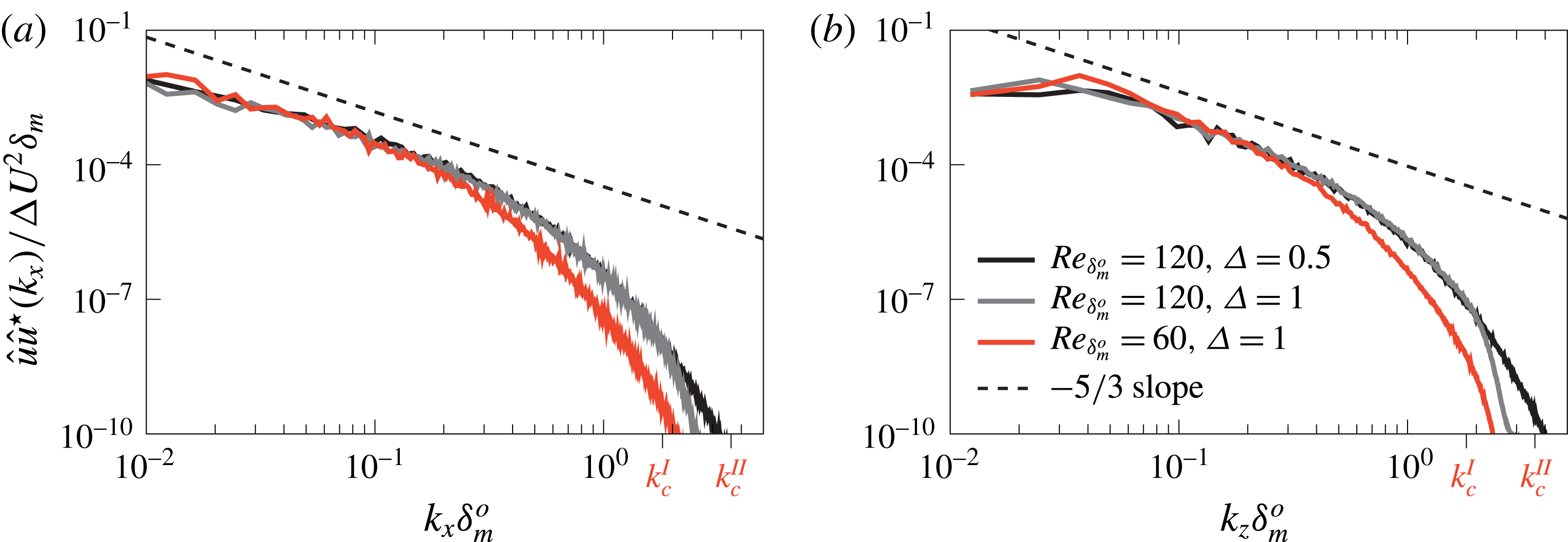
The $u$ -velocity spectra in figure 6 show that the turbulence has developed to be realistically broadband. The energy in the wavenumbers beyond $k\unicode[STIX]{x1D6FF}_{m}\gtrsim 10$ also decreases with increasing $M$ , which is consistent with compressible mixing-layer simulations at similar Mach numbers (Pantano & Sarkar Reference Pantano and Sarkar2002). For $Re_{\unicode[STIX]{x1D6FF}_{m}^{o}}=60$ and $120$ , the spectra overlay for $k\unicode[STIX]{x1D6FF}_{m}^{o}<0.01$ (figure 7), with more energy in the higher Reynolds number case for $k\unicode[STIX]{x1D6FF}_{m}^{o}\gtrsim 0.03$ . We further confirm sufficiency of the resolution by comparing a coarser mesh $\unicode[STIX]{x1D6E5}=\unicode[STIX]{x1D6FF}_{m}^{o}$ representation for $Re_{\unicode[STIX]{x1D6FF}_{m}^{o}}=120$ . Similarly, the negligible effect on the spectra of the numerical filter introduced in § 2 is confirmed in the Appendix.

Figure 6.

Spectrum of $u$ -velocity for all cases as indicated at $y=0$ when $\unicode[STIX]{x1D6FF}_{m}(t)/\unicode[STIX]{x1D6FF}_{m}^{o}=30$ in the (a) streamwise and (b) spanwise direction. The discrete Fourier transform of the $u$ -velocity is denoted $\hat{u}$ and its corresponding complex conjugate $\hat{u} ^{\star }$ . The wavenumber $k_{c}$ corresponds to a $1$ per cent damping due to the numerical filter discussed in § 2.

Figure 7.

Spectrum of $u$ -velocity for different Reynolds numbers as indicated for $M=2.5$ at $y=0$ when $\unicode[STIX]{x1D6FF}_{m}(t)/\unicode[STIX]{x1D6FF}_{m}^{o}=30$ in the (a) streamwise and (b) spanwise directions.

4 The near acoustic field

4.1 Pressure intensity

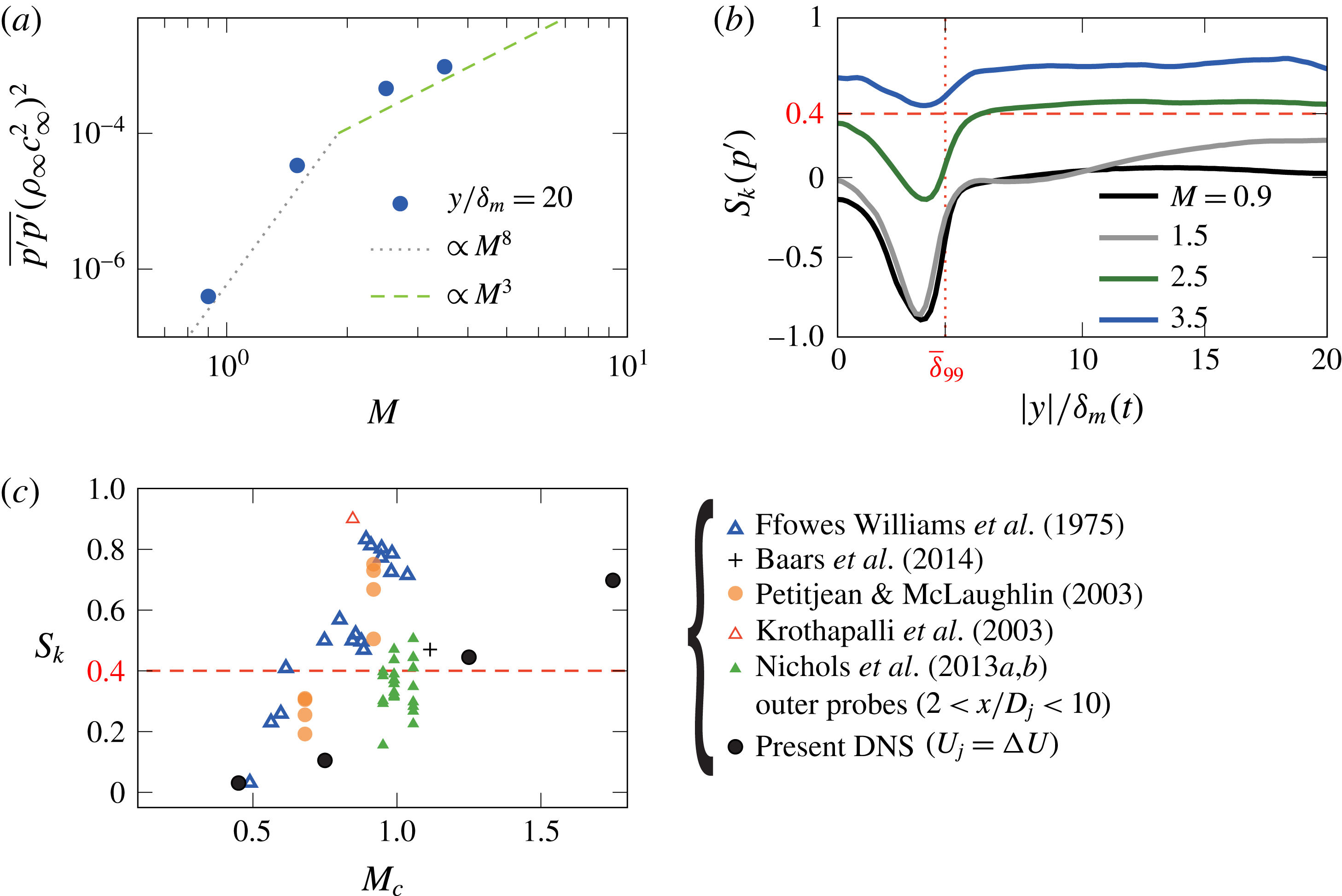
The radiated sound intensity is expected to change it scaling from $\langle p^{\prime }p^{\prime }\rangle \propto U_{j}^{8}$ to $\langle p^{\prime }p^{\prime }\rangle \propto U_{j}^{3}$ for $M\gtrsim 2$ , as anticipated by Ffowcs Williams (Reference Ffowcs Williams1963) and seen in experiments (Chobotov & Powell Reference Chobotov and Powell1957; Tanna, Dean & Burrin Reference Tanna, Dean and Burrin1976). Figure 8 confirms that the simulated intensity $\langle p^{\prime }p^{\prime }\rangle$ is consistent with this behaviour, and likewise shows the significant increase in intensity, which is important for any sound field nonlinearities.

Figure 8.

(a) Effect of Mach number on the pressure intensity. (b) Pressure skewness with distance from the mixing layer, with the dashed line showing the nominal crackle threshold $S_{k}=0.4$ and dotted line denoting the average $\unicode[STIX]{x1D6FF}_{99}$ and (c)  $y$ -averaged $S_{k}$ compared with experiments and simulations with $M_{c}=U_{j}/(c_{j}+c_{\infty })$ for the jets and $M_{c}$ from (3.1) for the present mixing layers.

4.2 Pressure traces

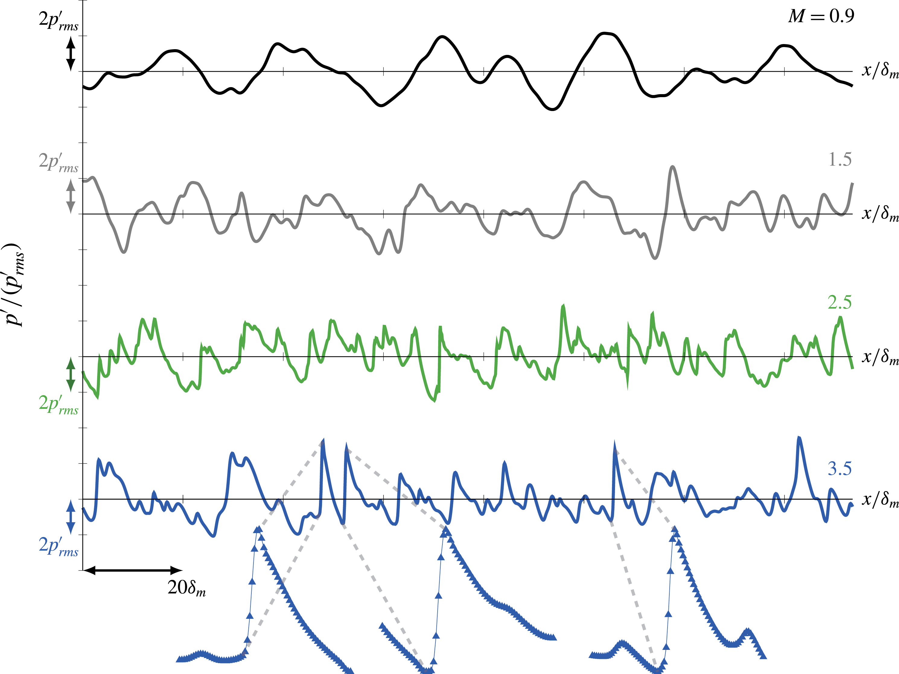
Figure 9 shows example sound-field pressure profiles for the different $M$ . For $M\lesssim 1.5$ , there are no obvious sharp peaks or shock-like compressions, and peaks and valleys appear to be symmetric about $p^{\prime }=0$ . In contrast, for $M\gtrsim 2.5$ , stronger $+p^{\prime }$ than $-p^{\prime }$ become apparent, and there are distinct sharp-peaked shock-like compressions. We note that in laboratory measurements the pressure is only typically acquired for $r\gtrsim 10D_{j}$ and often only for $r>100D_{j}$ (Ffowcs Williams et al. Reference Ffowcs Williams, Simson and Virchis1975; Petitjean et al. Reference Petitjean, Viswanathan and McLaughlin2006; Schlinker et al. Reference Schlinker, Simonich, Reba, Colonius and Ladeinde2008; Gee et al. Reference Gee, Neilsen and Atchley2013a ; Baars & Tinney Reference Baars and Tinney2014; Mora et al. Reference Mora, Heeb, Kastner, Gutmark and Kailasanath2014). Thus, the current pressure, with its steepened skewed features, suggests that this character manifests immediately adjacent the turbulent source, as seen in simulations of turbulent jets (Freund et al. Reference Freund, Lele and Moin2000; Nichols et al. Reference Nichols, Lele and Spyropoulos2013b ).

Figure 9.

Pressure variation with $x$ at $y/\unicode[STIX]{x1D6FF}_{m}(t)=5$ and $z=0$ when $\unicode[STIX]{x1D6FF}_{m}(t)/\unicode[STIX]{x1D6FF}_{m}^{o}=10$ . Since there are $N_{x}=1536$ mesh points in $x$ , even the sharpest features in these profiles are resolved, as shown with symbols marking mesh points for three features of the most challenging $M=3.5$ case.

4.3 Pressure skewness

Figure 8(b) shows that $S_{k}$ increases with $M$ at all $y$ . There does not appear to be a distinct transition to a finite $S_{k}$ (and nominally ‘crackling’ behaviour), though the $M$ -cases simulated do not necessarily preclude some sort of jump to finite $S_{k}$ for $M\approx 1.5$ . For $M=1.5$ , a slight increase in $S_{k}$ with $y$ beyond the rotational region suggests a weak propagation effect, but the $S_{k}$ levels still remain below those associated with crackle. For $M\gtrsim 2.5$ , $S_{k}$ exceeds $0.4$ . The sharpness of the sound field features for $M\geqslant 2.5$ in figure 9 raises concerns about their resolution; insensitivity to both Reynolds number and numerical dissipation is confirmed in the Appendix.

Since $S_{k}$ is nearly constant for $\unicode[STIX]{x1D6FF}_{99}<y/\unicode[STIX]{x1D6FF}_{m}<20$ , as seen in figure 8(b), we also average in the $y$ -direction,

(4.1) $$\begin{eqnarray}{S_{k}}_{|y|>\unicode[STIX]{x1D6FF}_{99}}={\displaystyle \frac{1}{L_{y}-\unicode[STIX]{x1D6FF}_{99}}}\int _{|y|>\unicode[STIX]{x1D6FF}_{99}}^{L_{y}}S_{k}\,\text{d}y,\end{eqnarray}$$

and we observe a monotonic increase with $M$ in figure 8(c). Again, even in the near field, there is no distinct ‘switch’ to finite $S_{k}$ . However, the skewness increases more rapidly over $M=0.9$ to $2.5$ and slower between $2.5\lesssim M\lesssim 3.5$ . Superficially, the different pace that $S_{k}$ increases with $M$ can be anticipated from measurements that shows $S_{k}\propto p_{rms}^{\prime }$ (Ffowcs Williams et al. Reference Ffowcs Williams, Simson and Virchis1975), which is also confirmed for these simulations (Buchta Reference Buchta2016). In this case, seeing the $p^{\prime }$ intensity shown in figure 8(a) we might anticipate the decreasing sensitivity of $S_{k}$ to $M$ .

Figure 8(c) also compares the near-field average (4.1) to jet measurements. The jet values are somewhat larger than those in the DNS, although this might be anticipated if additional propagation can further enhance $S_{k}$ reported in cases (Szewczyk Reference Szewczyk1978; Petitjean et al. Reference Petitjean, Viswanathan and McLaughlin2006; Schlinker et al. Reference Schlinker, Simonich, Reba, Colonius and Ladeinde2008). The very-near-field average $S_{k}$ of the large-eddy simulation of Nichols et al. (Reference Nichols, Lele, Ham, Martens and Spyropoulos2013a ,Reference Nichols, Lele and Spyropoulos b ) are more consistent with the present simulations. The noise source is also more complex in jets, particularly the intense fluctuations at the close of the potential core, where a jet behaviour is expected to deviate most significantly from the approximate self-similarity of the present simulation. Regardless, the simulations do reproduce the key $p^{\prime }$ intensity and $S_{k}$ behaviour of jets.

4.4 Wave development

4.4.1 Visualizations

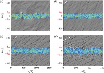
The visualizations in figure 10 show distinct Mach-like waves for $M\geqslant 2.5$ , with shock-like features propagating at distinct angles, which are shallower for $M=3.5$ . The $M=1.5$ case does not show such distinct sharp of features (figure 10 b), although the waves still have a distinct Mach-wave-like angle. For $M=0.9$ , no such waves are expected. As shown in the visualizations, the apparent wave angles match

(4.2) $$\begin{eqnarray}\unicode[STIX]{x1D703}=\sin ^{-1}\left({\displaystyle \frac{2c_{\infty }}{\unicode[STIX]{x0394}U+1}}\right),\end{eqnarray}$$

which is based on experimental data (Oertel Reference Oertel, Müller, Roesner and Schmidt1979).

Figure 10.

Two-dimensional plane at $z=L_{z}/2$ when $\unicode[STIX]{x1D6FF}_{m}/\unicode[STIX]{x1D6FF}_{m}^{o}=32$ : colours show vorticity magnitude ( $0.01<\left|\unicode[STIX]{x1D735}\times \boldsymbol{u}\right|\unicode[STIX]{x1D6FF}_{m}^{o}/\unicode[STIX]{x0394}U<0.25$ ) and greys show dilatation $(\unicode[STIX]{x1D735}\boldsymbol{\cdot }\boldsymbol{u})\unicode[STIX]{x1D6FF}_{m}^{o}/\unicode[STIX]{x0394}U$ for (a) $M=0.9$ , (b) $1.5$ , (c) $2.5$ and (d) $3.5$ . The dashed lines in (b–d) correspond to the Mach line orientation in (4.2). The dilatation grey levels span $\pm 0.002$ in (a), $\pm 0.005$ in (b) and $\pm 0.01$ in both (c) and (d).

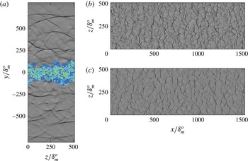
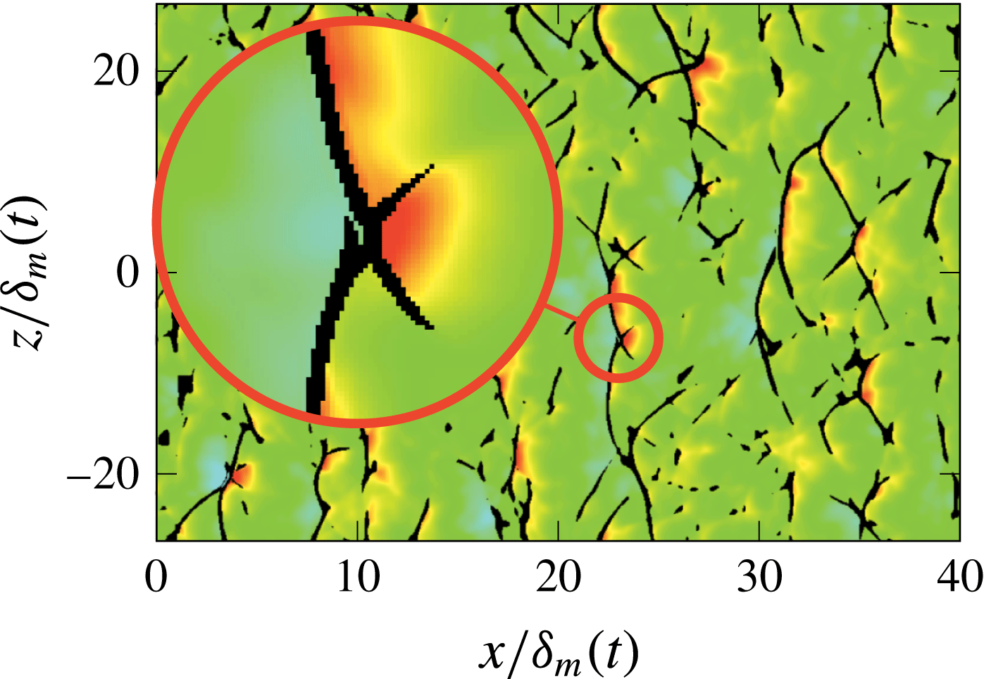
These two-dimensional visualizations, which suggest Mach waves that are similar to those radiated by high-speed projectiles or air vehicles, mask the surprisingly intricate three-dimensional structure of the near acoustic field seen in figure 11. Near to the turbulence, for $M\geqslant 2.5$ , the weak shocks are curved in the $z$ direction and form a cross-hatched pattern that flattens, as might be expected by nonlinear action, farther from the flow.

Figure 11.

(a) An $y$ – $z$ plane at $x=L_{x}/2$ when $\unicode[STIX]{x1D6FF}_{m}/\unicode[STIX]{x1D6FF}_{m}^{o}=32$ for $M=2.5$ : colours show vorticity magnitude with $0.01<\left|\unicode[STIX]{x1D735}\times \boldsymbol{u}\right|\unicode[STIX]{x1D6FF}_{m}^{o}/\unicode[STIX]{x0394}U<0.25$ and greys show dilatation $-0.01<(\unicode[STIX]{x1D735}\boldsymbol{\cdot }\boldsymbol{u})\unicode[STIX]{x1D6FF}_{m}^{o}/\unicode[STIX]{x0394}U<0.01$ . (b,c) Corresponding $x$ – $z$ planes visualized with the same levels at: (b) $y=7.5\unicode[STIX]{x1D6FF}_{m}$ and (c) $15\unicode[STIX]{x1D6FF}_{m}$ .

The corresponding pressure fluctuations visualized in figure 12 show the pressures are higher and particularly prominent where the compression waves intersect. A transport equation for $S_{k}$ is developed in § 5 quantifies the apparent lateral contributions of these interactions on $S_{k}$ .

Figure 12.

An $x$ – $z$ plane at $y=10\unicode[STIX]{x1D6FF}_{m}(t)$ when $\unicode[STIX]{x1D6FF}_{m}(t)/\unicode[STIX]{x1D6FF}_{m}^{o}=15$ showing pressure fluctuations for $M=2.5$ ; the colour varies with $p^{\prime }/\unicode[STIX]{x0394}U^{2}\unicode[STIX]{x1D70C}_{\infty }$ between $-0.3$ (blue) and $0.3$ (red), with the dilatation in black for $\unicode[STIX]{x1D735}\boldsymbol{\cdot }\boldsymbol{u}<1.25\times 10^{-2}\unicode[STIX]{x0394}U/\unicode[STIX]{x1D6FF}_{m}(t)$ .

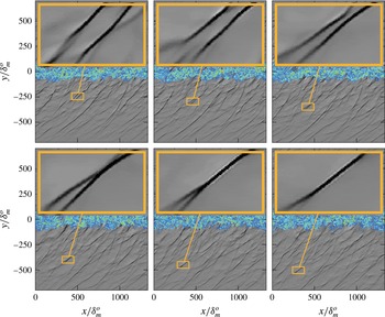
The instantaneous visualizations of the near-field sound also mask unsteady wave–wave interactions of the skewed pressure fields. Figure 13 shows a particular wave merging event, which is fundamentally nonlinear since linear waves would simply superpose. These are numerous throughout the near acoustic field, and seem to be more prevalent, as expected, for the greater nonlinearity of the more intense sound in the $M=3.5$ case. It is clear that the shear layer has grown little during the entire pictured sequence including this merging (approximately $30\,\%$ ). Thus, merging waves are generated at about the same mixing-layer thickness and are expected to share characteristics, as they would for a corresponding spatially developing flow. This, in turn, suggests that any such wave–wave interactions should closely resemble what would occur for spatially development. This is revisited in more detail in the following section.

Figure 13.

Example of wave merging for $M=2.5$ and $\unicode[STIX]{x1D6FF}_{m}(t)/\unicode[STIX]{x1D6FF}_{m}^{o}=19$ to $25$ at $z=L_{z}/2$ : colours show $|\unicode[STIX]{x1D735}\times \boldsymbol{u}|$ between $0.01$ and $0.25\unicode[STIX]{x0394}U/\unicode[STIX]{x1D6FF}_{m}^{o}$ and greys show $\unicode[STIX]{x1D735}\boldsymbol{\cdot }\boldsymbol{u}$ within $\pm 0.01\unicode[STIX]{x0394}U/\unicode[STIX]{x1D6FF}_{m}^{o}$ . Visualization are separated in time by $\unicode[STIX]{x0394}t=64\unicode[STIX]{x1D6FF}_{m}^{o}/c_{\infty }$ .

4.4.2 Wave statistics

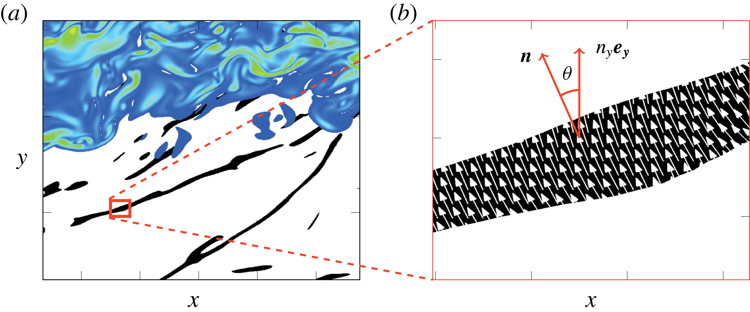
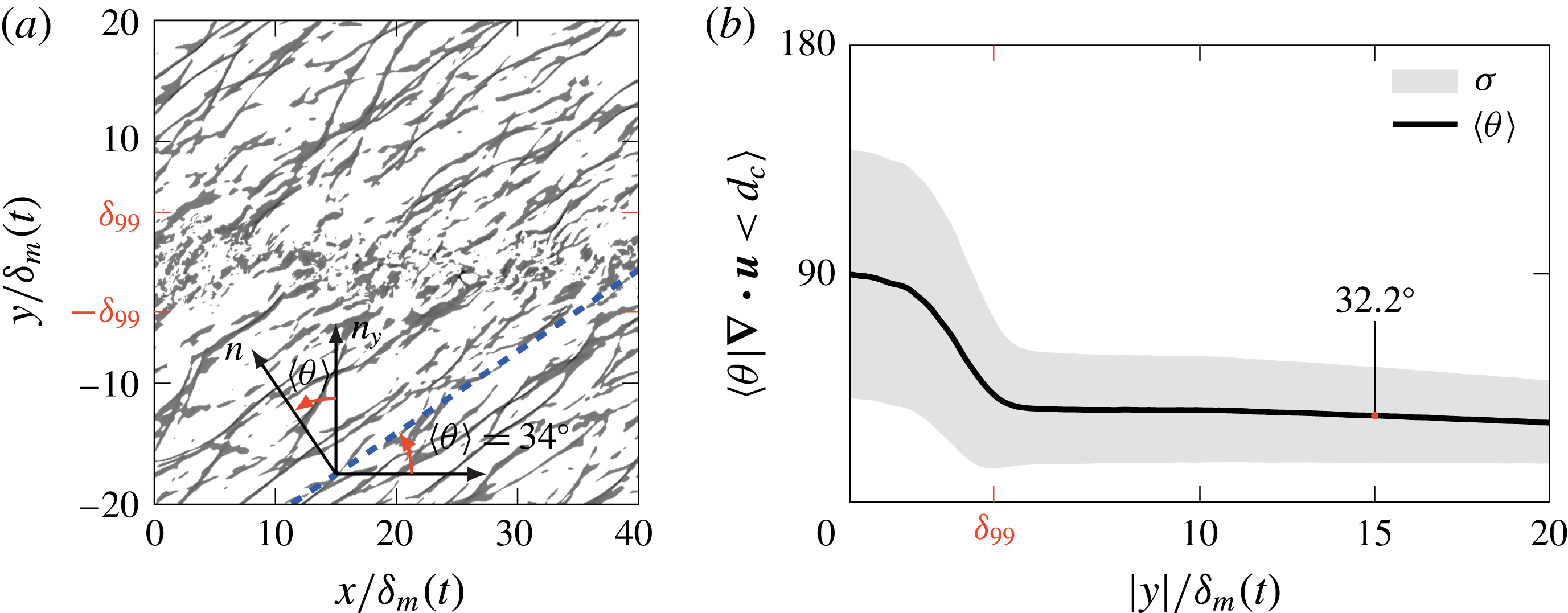
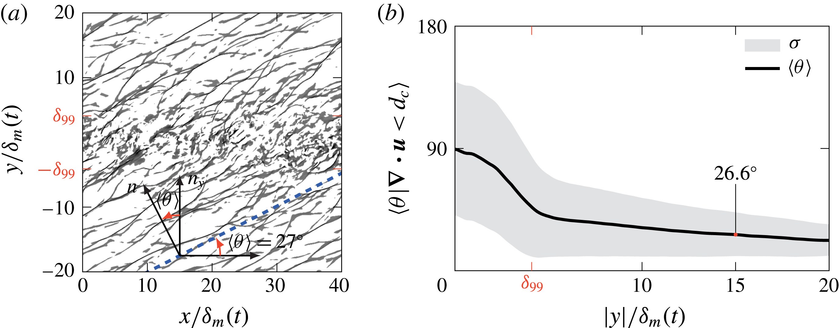
The near-field wave statistics quantify the mechanisms noted in the visualizations. We first consider wave angles, as shown in figure 14. To quantify this, we define the relatively strong compressions based on a threshold

(4.3) $$\begin{eqnarray}\unicode[STIX]{x1D735}\boldsymbol{\cdot }\boldsymbol{u}<d_{c}.\end{eqnarray}$$

The local angle with respect to the streamwise direction is then

(4.4) $$\begin{eqnarray}\unicode[STIX]{x1D703}=\cos ^{-1}n_{y},\end{eqnarray}$$

where $n_{y}$ is the $y$ -component of the normal vector

(4.5) $$\begin{eqnarray}\boldsymbol{n}={\displaystyle \frac{\unicode[STIX]{x1D735}p}{|\unicode[STIX]{x1D735}p|}}.\end{eqnarray}$$

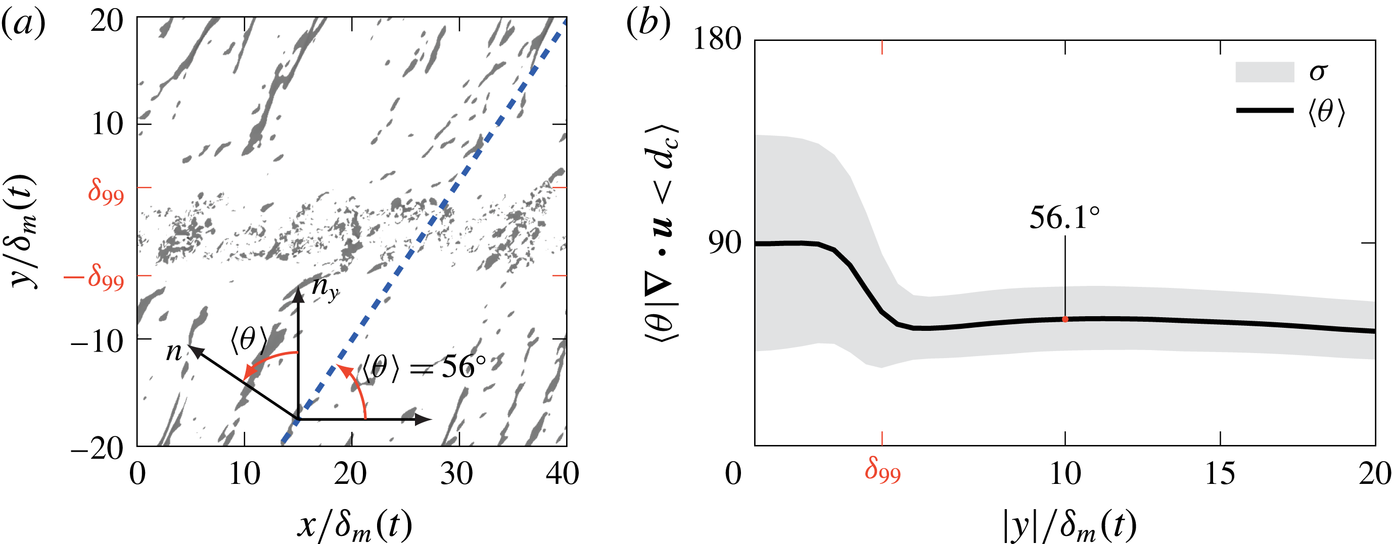
This angle is averaged conditionally over regions meeting the (4.3) criterion. Results presented in figures 15–17 used $d_{c}=-1.25\times 10^{-2}\unicode[STIX]{x0394}U/\unicode[STIX]{x1D6FF}_{m}(t)$ , and conclusions are insensitive to this particular value (Buchta Reference Buchta2016). The DNS results support an eddy advection hypothesis, with $\langle \unicode[STIX]{x1D703}\rangle =50.8^{\circ }$ , $31.3^{\circ }$ and $22.3^{\circ }$ at $y=20\,\unicode[STIX]{x1D6FF}_{m}(t)$ for $M=1.5$ , $2.5$ and $3.5$ , which are close to the corresponding $\unicode[STIX]{x1D703}=53^{\circ }$ , $35^{\circ }$ and $27^{\circ }$ from (4.2).

Of course, turbulence does not have a single, fixed advection speed. Thus, we also quantify the range of the wave angles by standard deviations of $\unicode[STIX]{x1D703}$ . The distributions are narrower at $M=1.5$ , similar to those observed by Murray & Lyons (Reference Murray and Lyons2016) for jet noise at similar conditions. For $M\geqslant 2.5$ the distributions narrow with increasing distance from the turbulence, and narrow more still at $M=3.5$ . This would be consistent with nonlinear merging of the kind visualized in figure 13. When weak shocks merge in this way, the resulting wave will have an angle between those of its constituents. This is similar to the geometric flattening and merging of weak shocks (Whitham Reference Whitham1974). Increased nonlinear interactions for the stronger perturbations for $M=3.5$ are thus expected to more rapidly narrow the distribution, as is indeed seen in figure 17(b).

Figure 14.

(a) The near acoustic field showing $\unicode[STIX]{x1D735}\boldsymbol{\cdot }\boldsymbol{u}<d_{c}$ as black and the adjacent turbulence with vorticity magnitude contours between $|\unicode[STIX]{x1D735}\times \boldsymbol{u}|=0.1$ and $5\,\unicode[STIX]{x0394}U/\unicode[STIX]{x1D6FF}_{m}(t)$ ; (b) a corresponding detailed view of the wavefront with the $x$ – $y$ components of $\boldsymbol{n}$ from (4.5) shown as vectors at the computational mesh point where the threshold (4.3) is satisfied.

Figure 15.

The $M=1.5$ case: (a) dilatation, $(\unicode[STIX]{x1D735}\boldsymbol{\cdot }\boldsymbol{u})\unicode[STIX]{x1D6FF}_{m}(t)/\unicode[STIX]{x0394}U<d_{c}$ , when $\unicode[STIX]{x1D6FF}_{m}(t)/\unicode[STIX]{x1D6FF}_{m}^{o}=15$ at $z=L_{z}/2$ , and (b) average wave angles $\langle \unicode[STIX]{x1D703}\rangle$ per (4.3) and shaded by one standard deviation $\unicode[STIX]{x1D70E}$ about the mean.

Figure 16.

Same as figure 15 for the $M=2.5$ case.

Figure 17.

Same as figure 15 for the $M=3.5$ case.

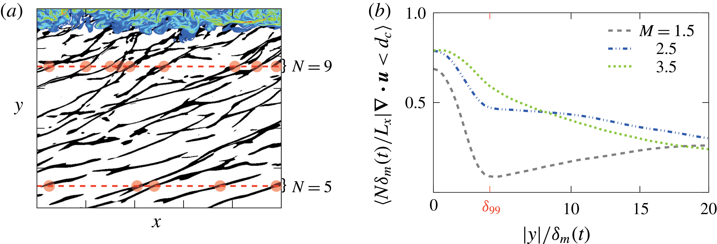
To quantify the rate of wave merging, we evaluate the number of distinct waves, which is expected to decrease with propagation distance (Lighthill Reference Lighthill, Batchelor and Davies1956) as stronger shocks with a higher propagation velocity overtake weaker ones (Lighthill Reference Lighthill, Batchelor and Davies1956, Reference Lighthill and Fung1993). Recent measurements also suggest the existence of wave merging (Fiévet et al. Reference Fiévet, Tinney, Baars and Hamilton2015). We count waves as the number of distinct compression regions that satisfy the threshold (4.3) at any $y$ -position, as illustrated in figure 18 (a). The result is shown in figure 18(b). We see a different evolution of wave density between the $M=1.5$ and the nominally crackling cases, $M=2.5$ and $3.5$ . The wave density is expected to increase with $y$ due to a retarded-time effect: at earlier times and smaller $\unicode[STIX]{x1D6FF}_{m}(t)$ the smaller scales of the turbulence should produce more compression waves. At larger $y$ , these earlier radiated shorter waves (and higher frequencies) will lead to there being more waves. Nonlinear merging counters this behaviour. For $M=2.5$ and $3.5$ , nonlinear merging overwhelms any retarded-time effect, and the number of waves decreases with distance from the mixing layer, doing so more rapidly for $M=3.5$ .

The temporal spreading of the mixing layers introduces two potential differences from the corresponding spatially developing flow. The first is relatively simple: similarity suggests that the mixing layer will radiate waves with increasing wavelength as it spreads in time, which is not the case for a fixed location in a spatially developing mixing layer. However, visualizations such as figure 18(a) suggest that the change in wave-to-wave spacing is slow, which is confirmed by the number density quantified in figure 18(b). The second consideration is more subtle and involves retarded-time effects. Self-similar development implies an origin at some time $\unicode[STIX]{x1D70F}=0$ . This early development was not simulated, although its extent would be small compared to the times simulated. For example, for the $M=3.5$ case with growth rate $\dot{\unicode[STIX]{x1D6FF}}_{m}/\unicode[STIX]{x1D6FF}_{m}^{o}\approx 0.008$ , our simulation omits the time range $-110\leqslant t\unicode[STIX]{x0394}U/\unicode[STIX]{x1D6FF}_{m}^{o}\leqslant 0$ during which the shear-layer thickness would have grown (if assumed linear) from $\unicode[STIX]{x1D6FF}_{m}(t)=0$ to $\unicode[STIX]{x1D6FF}_{m}(0)=\unicode[STIX]{x1D6FF}_{m}^{o}$ . If such data were available, similarity would indicate that waves would be more and more closely spaced closer to the $\unicode[STIX]{x1D70F}=0$ causality limit. To estimate the consequence of this for the region that we consider close to the mixing layer, we recognize that the similarity-scaled wave density at the point of generation ( $y\approx 0$ ) should be constant: $N^{\prime }(0)\equiv N(0)\unicode[STIX]{x1D6FF}_{m}(\unicode[STIX]{x1D70F})=C$ , where $C$ is the rate of Mach-wave generation. The main assumption here, consistent with self-similarity, is that the number of waves generated is inversely proportional to the mixing-layer thickness at the time of generation. Self-similarity also indicates $\unicode[STIX]{x1D6FF}_{m}(\unicode[STIX]{x1D70F})=\dot{\unicode[STIX]{x1D6FF}}_{m}\unicode[STIX]{x1D70F}$ with constant $\dot{\unicode[STIX]{x1D6FF}}_{m}$ . Taking advantage of the relatively regular Mach-wave structure of the radiation, we assume a speed $c_{y}$ of wave propagation in the $y$ direction ( $c_{y}\approx c_{\infty }\cos \unicode[STIX]{x1D703}$ ). With this, the wave density at $y=y_{o}$ is

(4.6) $$\begin{eqnarray}N^{\prime }(y_{o}^{\prime })={\displaystyle \frac{C}{1-{\displaystyle \frac{\dot{\unicode[STIX]{x1D6FF}}_{m}}{c_{y}}}y_{o}^{\prime }}},\end{eqnarray}$$

where $y_{o}^{\prime }=y_{o}/\unicode[STIX]{x1D6FF}_{m}(t)$ is a similarity coordinate, such as used in figure 17(a). This shows that for $y_{o}^{\prime }\ll c_{y}/\dot{\unicode[STIX]{x1D6FF}}_{m}$ the wave density of the current simulations, where quantified, should correspond to the sound radiated by a $\dot{\unicode[STIX]{x1D6FF}}_{m}=0$ spatially developing flow. The consequences for our reported observations are small. It most affects the $M=1.5$ results, for which wave angle of $\unicode[STIX]{x1D703}=50.8^{\circ }$ ( $c_{y}\approx 0.63\,c_{\infty }$ ) and $\dot{\unicode[STIX]{x1D6FF}}_{m}=0.006\,c_{\infty }$ leads to a 23 per cent increase at our maximum $y/\unicode[STIX]{x1D6FF}_{m}=20$ (e.g. figure 18 b). This is likely in part responsible for the increasing wave count with distance. For $M=3.5$ , the same comparison with $\dot{\unicode[STIX]{x1D6FF}}_{m}=0.002\,c_{\infty }$ and $\unicode[STIX]{x1D703}=22^{\circ }$ yields only a 5 per cent increase. So retarded-time effects do increase wave density in $y$ as observed for $M=1.5$ , although only weakly, especially weakly at smaller $y$ and larger $M$ . Nonlinear merging leads to the $y$ -decreasing wave density for $M\geqslant 2.5$ .

Figure 18.

(a) Example wave counts based on (4.3) and (b) the corresponding $y$ -dependence.

5 Transport of $S_{k}$

The visualizations and wave statistics show the effects of nonlinear propagation but do not address the $S_{k}$ values. To identify the factors that affect $S_{k}$ we develop a $S_{k}$ transport equation, as might be derived for Reynolds stresses or turbulence kinetic energy. We start with product-rule differentiation of pressure skewness advection using (1.1)

(5.1) $$\begin{eqnarray}{\displaystyle \frac{\overline{\text{D}}}{\text{D}t}}S_{k}\equiv {\displaystyle \frac{\overline{\text{D}}}{\text{D}t}}\left[{\displaystyle \frac{\overline{(p^{\prime })}^{3}}{\overline{(p^{\prime })^{2}}^{3/2}}}\right]=[\overline{(p^{\prime })^{2}}]^{-3/2}\left\{{\displaystyle \frac{\overline{\text{D}}}{\text{D}t}}\overline{(p^{\prime })^{3}}-{\displaystyle \frac{3}{2}}{\displaystyle \frac{\overline{(p^{\prime })^{3}}}{\overline{(p^{\prime })^{2}}}}{\displaystyle \frac{\overline{\text{D}}}{\text{D}t}}\overline{(p^{\prime })^{2}}\right\},\end{eqnarray}$$

where

(5.2) $$\begin{eqnarray}{\displaystyle \frac{\overline{\text{D}}}{\text{D}t}}()\equiv {\displaystyle \frac{\unicode[STIX]{x2202}}{\unicode[STIX]{x2202}t}}+\overline{v}{\displaystyle \frac{\unicode[STIX]{x2202}}{\unicode[STIX]{x2202}y}},\end{eqnarray}$$

has only a $y$ -advection component since the turbulence is statistically homogeneous in the $x$ - and $z$ -directions. We further develop (5.1) based on evolution equations for $\overline{(p^{\prime })^{3}}$ and $\overline{(p^{\prime })^{2}}$ , and for this we begin with an equation for pressure

(5.3) $$\begin{eqnarray}{\displaystyle \frac{\unicode[STIX]{x2202}p}{\unicode[STIX]{x2202}t}}=-u_{i}{\displaystyle \frac{\unicode[STIX]{x2202}p}{\unicode[STIX]{x2202}x_{i}}}-\unicode[STIX]{x1D6FE}p{\displaystyle \frac{\unicode[STIX]{x2202}u_{i}}{\unicode[STIX]{x2202}x_{i}}}+{\mathcal{D}},\end{eqnarray}$$

which is an exact consequence of the governing flow equations. For compactness, the heat conduction and viscous terms are combined in

(5.4) $$\begin{eqnarray}{\mathcal{D}}=(\unicode[STIX]{x1D6FE}-1)\left\{{\displaystyle \frac{1}{Re_{\unicode[STIX]{x1D6FF}_{m}^{o}}Pr}}{\displaystyle \frac{\unicode[STIX]{x2202}^{2}T}{\unicode[STIX]{x2202}x_{i}\unicode[STIX]{x2202}x_{i}}}+\unicode[STIX]{x1D70F}_{ij}{\displaystyle \frac{\unicode[STIX]{x2202}u_{i}}{\unicode[STIX]{x2202}x_{j}}}\right\}\end{eqnarray}$$

and the viscous stress is

(5.5) $$\begin{eqnarray}\unicode[STIX]{x1D70F}_{ij}={\displaystyle \frac{1}{Re_{\unicode[STIX]{x1D6FF}_{m}^{o}}}}\left({\displaystyle \frac{\unicode[STIX]{x2202}u_{i}}{\unicode[STIX]{x2202}x_{j}}}+{\displaystyle \frac{\unicode[STIX]{x2202}u_{j}}{\unicode[STIX]{x2202}x_{i}}}-{\displaystyle \frac{2}{3}}{\displaystyle \frac{\unicode[STIX]{x2202}u_{k}}{\unicode[STIX]{x2202}x_{k}}}\unicode[STIX]{x1D6FF}_{ij}\right).\end{eqnarray}$$

In (5.4), the Prandtl number is $Pr=0.71$ and $Re_{\unicode[STIX]{x1D6FF}_{m}^{o}}$ from (2.2). In forming (5.3), the following non-dimensionalization was used:

(5.6) $$\begin{eqnarray}\left.\begin{array}{@{}c@{}}\unicode[STIX]{x1D70C}={\displaystyle \frac{\unicode[STIX]{x1D70C}^{\star }}{\unicode[STIX]{x1D70C}_{\infty }}},\quad u_{i}={\displaystyle \frac{u_{i}^{\star }}{\unicode[STIX]{x0394}U}},\quad p={\displaystyle \frac{p^{\star }}{\unicode[STIX]{x1D70C}_{\infty }\unicode[STIX]{x0394}U^{2}}},\quad T={\displaystyle \frac{T^{\star }c_{p}^{\star }}{\unicode[STIX]{x0394}U^{2}}},\\ x={\displaystyle \frac{x^{\star }}{\unicode[STIX]{x1D6FF}_{m}^{o}}},\quad \text{and}\quad t={\displaystyle \frac{t^{\star }\unicode[STIX]{x1D6FF}_{m}^{o}}{\unicode[STIX]{x0394}U}},\end{array}\right\}\end{eqnarray}$$

where ( $^{\star }$ ) quantities represent dimensional values. Reynolds decomposing the pressure and velocity,

(5.7) $$\begin{eqnarray}\displaystyle & \displaystyle p(\boldsymbol{x},t)=\overline{p}(y,t)+p^{\prime }(\boldsymbol{x},t) & \displaystyle\end{eqnarray}$$

(5.8) $$\begin{eqnarray}\displaystyle & \displaystyle u_{i}(\boldsymbol{x},t)=\overline{u}_{i}(y,t)+u_{i}^{\prime }(\boldsymbol{x},t), & \displaystyle\end{eqnarray}$$

in (5.3) and averaging yields the mean pressure equation

(5.9) $$\begin{eqnarray}{\displaystyle \frac{\unicode[STIX]{x2202}\overline{p}}{\unicode[STIX]{x2202}t}}+\overline{u_{i}}{\displaystyle \frac{\unicode[STIX]{x2202}\overline{p}}{\unicode[STIX]{x2202}x_{i}}}+\overline{u_{i}^{\prime }{\displaystyle \frac{\unicode[STIX]{x2202}p^{\prime }}{\unicode[STIX]{x2202}x_{i}}}}=-\unicode[STIX]{x1D6FE}\left[\overline{p}{\displaystyle \frac{\unicode[STIX]{x2202}\overline{u_{i}}}{\unicode[STIX]{x2202}x_{i}}}+\overline{p^{\prime }{\displaystyle \frac{\unicode[STIX]{x2202}u_{i}^{\prime }}{\unicode[STIX]{x2202}x_{i}}}}\right]+\overline{{\mathcal{D}}}.\end{eqnarray}$$

Substituting in (5.3) and (5.9) into

(5.10) $$\begin{eqnarray}{\displaystyle \frac{\unicode[STIX]{x2202}p^{\prime }}{\unicode[STIX]{x2202}t}}={\displaystyle \frac{\unicode[STIX]{x2202}p}{\unicode[STIX]{x2202}t}}-{\displaystyle \frac{\unicode[STIX]{x2202}\overline{p}}{\unicode[STIX]{x2202}t}},\end{eqnarray}$$

yields

(5.11) $$\begin{eqnarray}{\displaystyle \frac{\unicode[STIX]{x2202}p^{\prime }}{\unicode[STIX]{x2202}t}}=-\overline{u_{i}}{\displaystyle \frac{\unicode[STIX]{x2202}p^{\prime }}{\unicode[STIX]{x2202}x_{i}}}-u_{i}^{\prime }{\displaystyle \frac{\unicode[STIX]{x2202}\overline{p}}{\unicode[STIX]{x2202}x_{i}}}-u_{i}^{\prime }{\displaystyle \frac{\unicode[STIX]{x2202}p^{\prime }}{\unicode[STIX]{x2202}x_{i}}}+\overline{u_{i}^{\prime }{\displaystyle \frac{\unicode[STIX]{x2202}p^{\prime }}{\unicode[STIX]{x2202}x_{i}}}}-\unicode[STIX]{x1D6FE}\left[\overline{p}{\displaystyle \frac{\unicode[STIX]{x2202}u_{i}^{\prime }}{\unicode[STIX]{x2202}x_{i}}}+p^{\prime }{\displaystyle \frac{\unicode[STIX]{x2202}\overline{u_{i}}}{\unicode[STIX]{x2202}x_{i}}}+p^{\prime }{\displaystyle \frac{\unicode[STIX]{x2202}u_{i}^{\prime }}{\unicode[STIX]{x2202}x_{i}}}-\overline{p^{\prime }{\displaystyle \frac{\unicode[STIX]{x2202}u_{i}^{\prime }}{\unicode[STIX]{x2202}x_{i}}}}\right]+{\mathcal{D}}^{\prime },\end{eqnarray}$$

where the fluctuating viscous and heat conduction term is ${\mathcal{D}}^{\prime }={\mathcal{D}}-\overline{{\mathcal{D}}}$ . Since

(5.12) $$\begin{eqnarray}{\displaystyle \frac{\unicode[STIX]{x2202}\overline{(p^{\prime })^{3}}}{\unicode[STIX]{x2202}t}}=\overline{3(p^{\prime })^{2}{\displaystyle \frac{\unicode[STIX]{x2202}p^{\prime }}{\unicode[STIX]{x2202}t}}},\end{eqnarray}$$

the first term on the right-hand side of (5.1) along with (5.11) and (5.12) gives

(5.13) $$\begin{eqnarray}\left.\begin{array}{@{}rclr@{}}\left[\overline{{p^{\prime }}^{2}}\right]^{-3/2}{\displaystyle \frac{\overline{\text{D}}}{\text{D}t}}\overline{{p^{\prime }}^{3}} & = & \left[\overline{{p^{\prime }}^{2}}\right]^{-3/2}\\ & & \times \,\bigg[-3\overline{v^{\prime }{p^{\prime }}^{2}}{\displaystyle \frac{\unicode[STIX]{x2202}\overline{p}}{\unicode[STIX]{x2202}y}} & (\text{Ia})\\ & & -\,\overline{{\displaystyle \frac{\unicode[STIX]{x2202}v^{\prime }{p^{\prime }}^{3}}{\unicode[STIX]{x2202}y}}} & (\text{IIa})\\ & & +\,3\overline{{p^{\prime }}^{2}}\overline{u_{i}^{\prime }{\displaystyle \frac{\unicode[STIX]{x2202}p^{\prime }}{\unicode[STIX]{x2202}x_{i}}}} & (\text{IIIa})\\ & & -\,3\unicode[STIX]{x1D6FE}\overline{p}\overline{{p^{\prime }}^{2}d^{\prime }} & (\text{IVa})\\ & & -\,3\unicode[STIX]{x1D6FE}\overline{{p^{\prime }}^{3}}{\displaystyle \frac{\unicode[STIX]{x2202}\overline{v}}{\unicode[STIX]{x2202}y}} & (\text{Va})\\ & & +\,(-3\unicode[STIX]{x1D6FE}+1)\overline{{p^{\prime }}^{3}d^{\prime }} & (\text{VIa})\\ & & +\,3\unicode[STIX]{x1D6FE}\overline{{p^{\prime }}^{2}}\cdot \overline{p^{\prime }d^{\prime }} & (\text{VIIa})\\ & & +\,3\overline{{p^{\prime }}^{2}{\mathcal{D}}^{\prime }}\quad \bigg]. & (\text{VIIIa})\end{array}\right\}\end{eqnarray}$$

Similarly, the second term on the right-hand side of (5.1) can be written

(5.14) $$\begin{eqnarray}\left.\begin{array}{@{}rclr@{}}-{\displaystyle \frac{3}{2}}{\displaystyle \frac{\overline{{p^{\prime }}^{3}}}{\overline{{p^{\prime }}^{2}}^{5/2}}}\times {\displaystyle \frac{\overline{\text{D}}}{\text{D}t}}\overline{{p^{\prime }}^{2}} & = & -{\displaystyle \frac{3}{2}}{\displaystyle \frac{\overline{{p^{\prime }}^{3}}}{\overline{{p^{\prime }}^{2}}^{5/2}}}\\ & & \times \,\bigg[-2\overline{v^{\prime }p^{\prime }}{\displaystyle \frac{\unicode[STIX]{x2202}\overline{p}}{\unicode[STIX]{x2202}y}} & (\text{Ib})\\ & & -\,2\overline{p^{\prime }u_{i}^{\prime }{\displaystyle \frac{\unicode[STIX]{x2202}p^{\prime }}{\unicode[STIX]{x2202}x_{i}}}} & (\text{IIb})\\ & & -\,2\unicode[STIX]{x1D6FE}\overline{p}\overline{p^{\prime }d^{\prime }} & (\text{IIIb})\\ & & -\,2\unicode[STIX]{x1D6FE}\overline{{p^{\prime }}^{2}}{\displaystyle \frac{\unicode[STIX]{x2202}\overline{v}}{\unicode[STIX]{x2202}y}} & (\text{IVb})\\ & & -\,2\unicode[STIX]{x1D6FE}\overline{{p^{\prime }}^{2}d^{\prime }} & (\text{Vb})\\ & & +\,2\overline{p^{\prime }{\mathcal{D}}^{\prime }}\bigg]. & (\text{VIb})\end{array}\right\}\end{eqnarray}$$

Together, the right-hand sides of (5.13) and (5.14) govern $S_{k}$ . We remark that positive-valued sources of pressure intensity in (5.14) are sinks of pressure skewness, which are due to the negative prefactor in (5.14). This is simply because $\overline{{p^{\prime }}^{2}}$ appears in the denominator of skewness in (5.1), so increasing $\overline{{p^{\prime }}^{2}}$ of itself will decrease $S_{k}$ . The collection of terms selected to form (5.13) and (5.14) is not unique but was deemed useful for the following discussion.

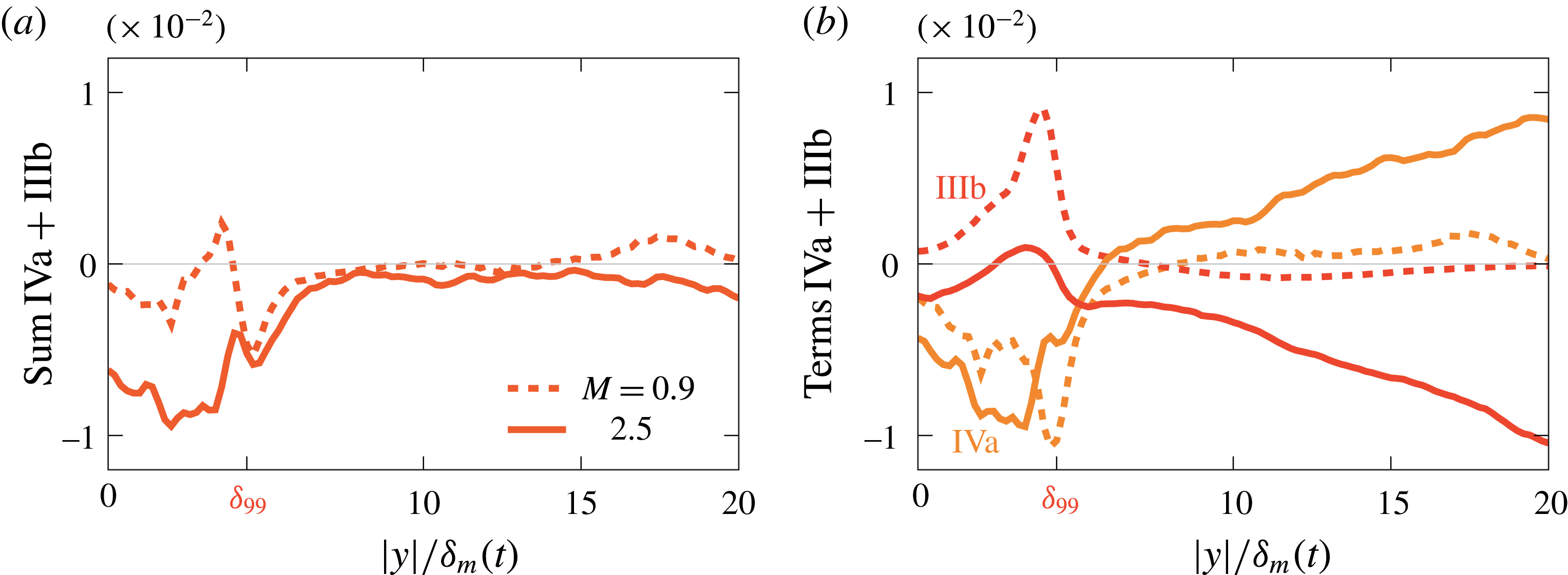
The complete description of these terms and their contributions are provided elsewhere (Buchta Reference Buchta2016). We summarize the main findings relevant to crackle and contrast them with the $S_{k}\approx 0$ , $M=0.9$ flow. As expected, all terms depending on gradients of the mean outside the shear region are negligible (terms Ia, Va, Ib and IVb). We also anticipated that IVa and IIIb, when summed

(5.15) $$\begin{eqnarray}\underbrace{-3\unicode[STIX]{x1D6FE}\overline{p}\overline{{p^{\prime }}^{2}d^{\prime }}\cdot \overline{{p^{\prime }}^{2}}^{-3/2}}_{(\text{IVa})}+\underbrace{3\unicode[STIX]{x1D6FE}\overline{p}\cdot \overline{p^{\prime }d^{\prime }}\cdot \overline{{p^{\prime }}^{3}}\cdot \overline{{p^{\prime }}^{2}}^{-5/2}}_{(\text{IIIb})}\end{eqnarray}$$

are also insignificant based on planar weak-shock theory. This follows from recognizing that the pressure increase across a viscous shock is (Taylor Reference Taylor1910; Lighthill Reference Lighthill, Batchelor and Davies1956; Thompson Reference Thompson1988)

(5.16) $$\begin{eqnarray}{\displaystyle \frac{p^{\prime }}{\unicode[STIX]{x1D70C}_{\infty }c_{\infty }^{2}}}=-{\displaystyle \frac{l_{s}d^{\prime }}{\unicode[STIX]{x0394}U}},\end{eqnarray}$$

where $l_{s}$ is a measure of the shock thickness. Thus, for any particular shock $p^{\prime }\propto -d^{\prime }$ and the two terms in (5.15) cancel. Furthermore, both are in proportion to $d^{\prime }$ , so these will contribute mostly within the strong (large $|d^{\prime }|$ ) compressions and much less away from them. Figure 19 confirms this for the simulation data: their sum in (a) is indeed significantly smaller than their individual contribution in (b). In the $M=0.9$ case, these correlations are negligible since weak shocks are absent.

Figure 19.

(a) The sum of terms (IVa) and (IIIb) in (5.13) and (5.14) for $M=0.9$ (dashed) and $2.5$ (solid). (b) The corresponding separate contributions.

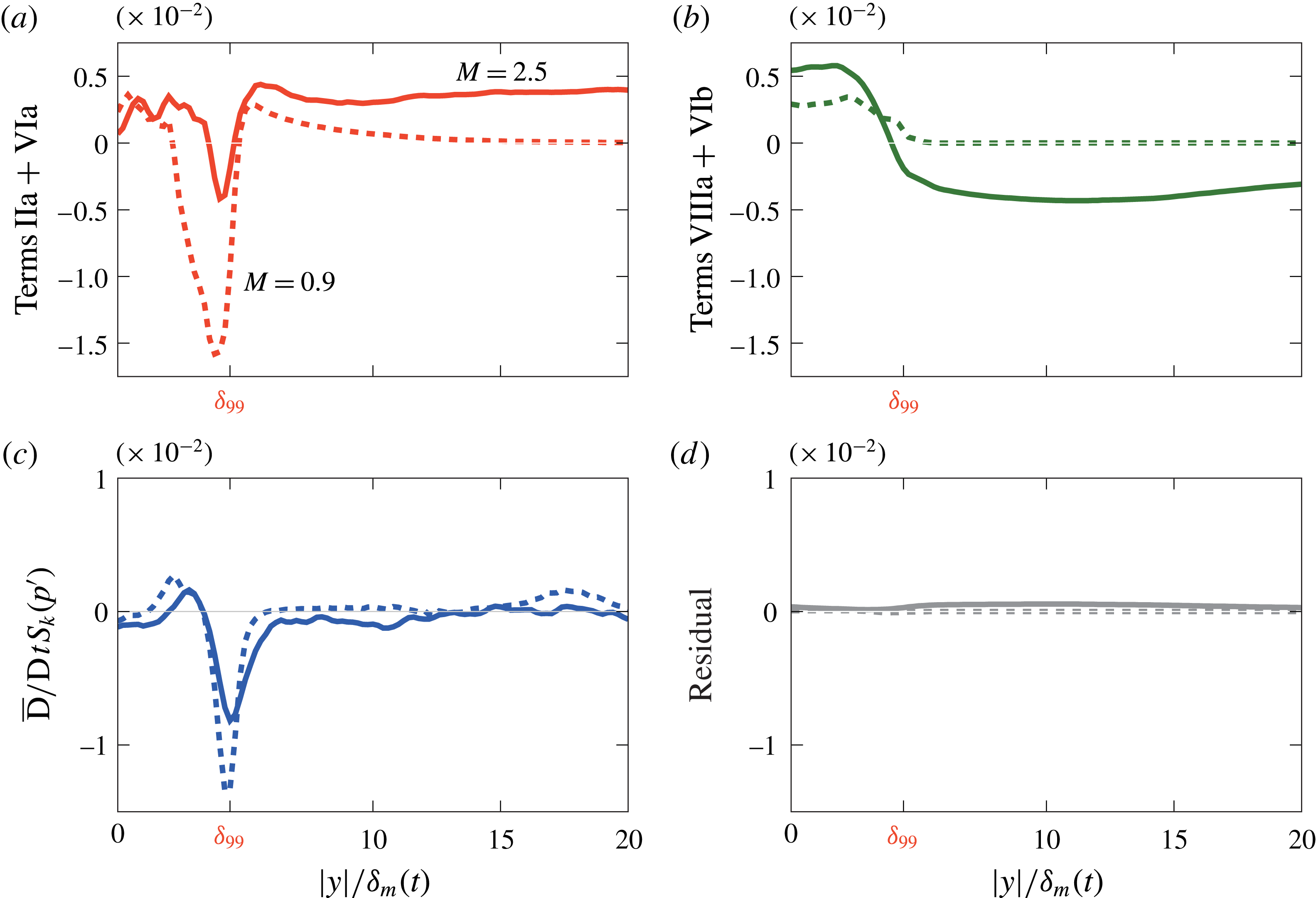
Figure 20(a,b) shows the main sources and sinks of $S_{k}$ transport. Beyond $y/\unicode[STIX]{x1D6FF}_{99}$ , the terms IIa  $+$  VIa, generating $S_{k},$ are balanced by dissipation effects (VIIIa  $+$  VIb) with correlations multiplying ${\mathcal{D}}^{\prime }$ . Term IIa has a flux-like form transporting $S_{k}$ , similar to the turbulence transport in an energy budget, and is not a true source such as VIa. For $M=0.9$ , these terms decay rapidly beyond $y=\unicode[STIX]{x1D6FF}_{99}$ , which is consistent with an approximately linear sound field. The source and dissipation terms are in near balance beyond $y/\unicode[STIX]{x1D6FF}_{m}\gtrsim \unicode[STIX]{x1D6FF}_{99}$ , as seen in figure 20(c), which is also consistent with the approximately constant $S_{k}$ (figure 8 b). Of course, small effects, indiscernible due to the finite statistical sample available here, could provide a small source of $S_{k}$ that is collectively significant over longer distances. All remaining terms are small. Figure 20(d) shows that the residual formed by subtracting the left- and right-hand sides of (5.1) is approximately ten times smaller than the primary budget terms in (a) and (b).

It might be anticipated that numerical dissipation acting on the shock thickness scale could affect the $S_{k}$ transport by enhancing dissipation in thin shock-like structures. However, over the range of Reynolds numbers, numerical filtering schedules tested (and seen in the spectra in figure 22), there were no discernible effects.

Figure 20.

Primary skewness budget terms: sources (IIa)  $+$  (VIa) in (a) and sinks (VIIIa)  $+$  (VIb) in (b). (c) The net transport of $S_{k}$ and (d) the residual between the left- and right-hand sides of (5.1).

The lateral ( $x$ – $z$ ) plane image of strong dilatation and pressure in figure 12 suggested the possibility a source of $S_{k}$ might arise at wave intersections above the turbulence. However, the lateral derivatives in $x$ and $z$ making up $d^{\prime }$ make almost no average contributions to the (VIa) source. This can be seen by recrafting (IIa)  $+$  (VIa) as

(5.17) $$\begin{eqnarray}\displaystyle & & \displaystyle \underbrace{{\displaystyle \frac{\unicode[STIX]{x2202}\overline{v^{\prime }{p^{\prime }}^{3}}}{\unicode[STIX]{x2202}y}}}_{(\text{IIa})}+\underbrace{(3\unicode[STIX]{x1D6FE}-1)\overline{{p^{\prime }}^{3}d^{\prime }}}_{(\text{IVa})}\nonumber\\ \displaystyle & & \displaystyle \qquad =3\unicode[STIX]{x1D6FE}{\displaystyle \frac{\unicode[STIX]{x2202}\overline{v^{\prime }{p^{\prime }}^{3}}}{\unicode[STIX]{x2202}y}}+(-3\unicode[STIX]{x1D6FE}+1)\overline{v^{\prime }{\displaystyle \frac{\unicode[STIX]{x2202}{p^{\prime }}^{3}}{\unicode[STIX]{x2202}y}}}+(3\unicode[STIX]{x1D6FE}-1)\overline{{p^{\prime }}^{3}\left\{{\displaystyle \frac{\unicode[STIX]{x2202}u^{\prime }}{\unicode[STIX]{x2202}x}}+{\displaystyle \frac{\unicode[STIX]{x2202}w^{\prime }}{\unicode[STIX]{x2202}z}}\right\}}\end{eqnarray}$$

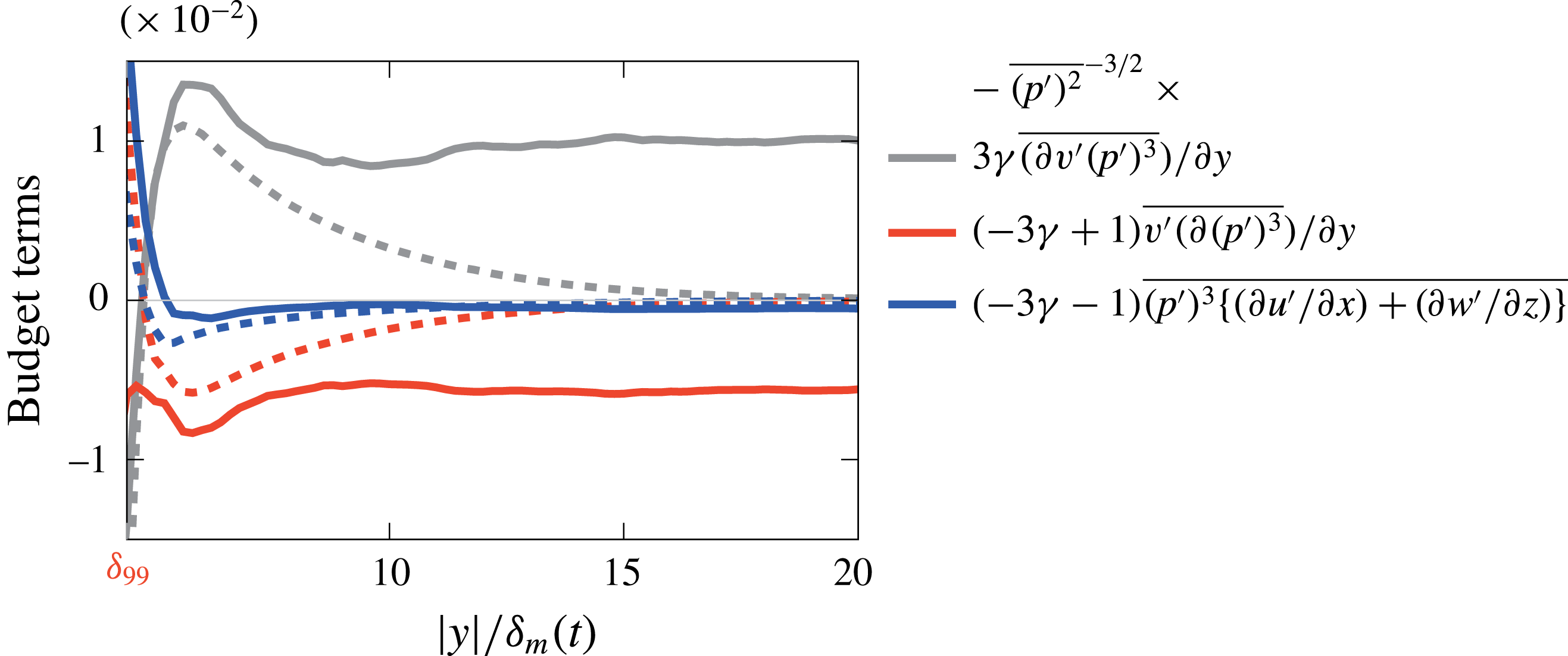
and their contributions shown in figure 21. The $S_{k}$ beyond the rotational region is primarily due to $\unicode[STIX]{x2202}_{y}(v^{\prime }{p^{\prime }}^{3})$ and balanced in part by $v^{\prime }\unicode[STIX]{x2202}_{y}({p^{\prime }}^{3})$ with essentially no contributions from terms with streamwise and spanwise velocity derivatives in (5.17). These data suggest that the curved, intersecting waves shown in figure 12 can form strong peaks, yet ultimately they are not contributing as a $S_{k}$ source.

Figure 21.

Individual contributions of (IIa) and (VIa) in (5.13) from (5.17) for $M=0.9$ (dashed) and $2.5$ (solid).

Figure 22.

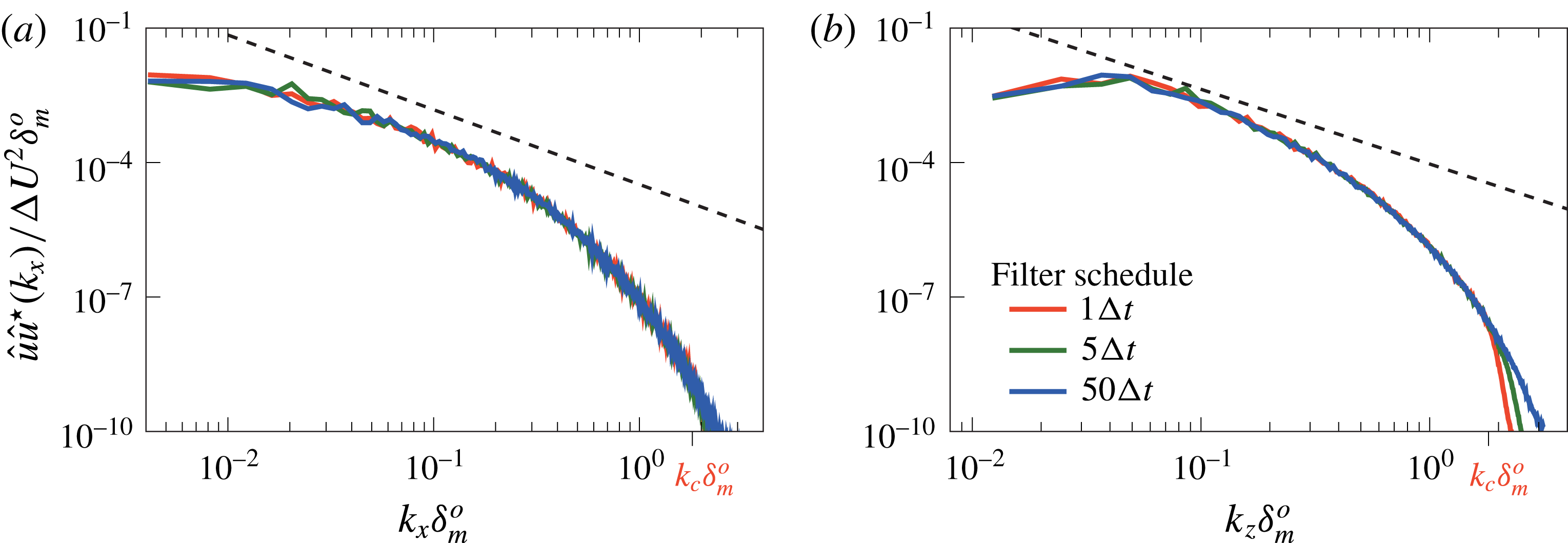
Effect of the numerical filter on the midplane ( $y=0$ ) $u$ -velocity spectra in the (a) streamwise and (b) spanwise direction.