1. Introduction
From nature to industry, wetting and dewetting flow structures occur in various hydrodynamic problems (Bonn et al. Reference Bonn, Eggers, Indekeu, Meunier and Rolley2009). When describing the flow of a continuous fluid near the contact line using a simple wedge shape, a well-known issue arises: the stress and pressure diverge if we adhere to the no-slip boundary condition (Huh & Scriven Reference Huh and Scriven1971). This makes it difficult to provide a fundamental description of moving contact lines. Alternatively, to clarify the phenomena near the moving contact line, non-continuum models are used. For instance, molecular dynamics (MD) simulations (Gentner, Ogonowski & De Coninck Reference Gentner, Ogonowski and De Coninck2003; Blake Reference Blake2006) and lattice-Boltzmann (LB) simulations (Blake, De Coninck & d’Ortona Reference Blake, De Coninck and d’Ortona1995; Mo, Liu & Kwok Reference Mo, Liu and Kwok2005) are used to study mechanism of contact line dynamics. These simulations are well suited to study microscopic systems (Bonn et al. Reference Bonn, Eggers, Indekeu, Meunier and Rolley2009).
From a hydrodynamic point of view, two approaches have been introduced to resolve the singularity issue: either a slip boundary condition at the contact line is applied (Brochard-Wyart & De Gennes Reference Brochard-Wyart and De Gennes1992), or a partial wetting structure near a contact line is assumed between the macroscopic layer and the thin film (De Gennes Reference De Gennes1985). The Navier–Stokes equations can be used to study the wetting and dewetting dynamics problem, provided that boundary conditions are properly formulated.
To study wetting and dewetting flow problems, classical lubrication theory is a useful approach to simplify the governing equations. When
 $\mathit{Re}\,{\it\epsilon}$
is much smaller than unity, the flow field can be assumed to be in the Stokes regime, i.e. with negligible nonlinear convective acceleration terms (Reynolds Reference Reynolds1886; White Reference White2005). Here,
 $\mathit{Re}$
(
 $={\it\rho}Uh_{f}/{\it\mu}$
;
 ${\it\rho}$
denotes density,
 $U$
the substrate speed,
 $h_{f}$
the droplet tail height,
 ${\it\mu}$
the viscosity) is the Reynolds number and
 ${\it\epsilon}$
(
 $=h_{f}/L$
;
 $L$
the streamwise length) represents the aspect ratio of the flow geometry.
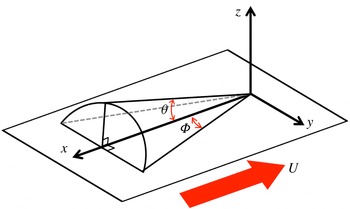
Limat & Stone (Reference Limat and Stone2004) introduced a three-dimensional lubrication model for the dewetting corner structure of a droplet sliding down on an inclined substrate in the framework of lubrication theory. They used a similarity solution to describe the contact line shape of the three-dimensional structure near the corner singularity. Then, they showed that two angles (see definitions of the angles in figure 1), namely the dynamic receding contact angle
 ${\it\theta}$
and the half-opening angle
 ${\rm\Phi}$
, are linked to each other. Furthermore, based on this model, Snoeijer et al. (Reference Snoeijer, Rio, Le Grand and Limat2005) obtained an analytical solution for the internal flow field near the corner structure, which showed a self-similar flow pattern. These models are limited to low Reynolds number (
 $\mathit{Re}\ll 1$
) and low dynamic receding contact angle (
 ${\it\theta}<20^{\circ }$
).
Sketch of the dewetting corner geometry.

Interestingly, qualitatively similar results are observed in flows where the conventional lubrication approximation no longer holds, i.e.
 $\mathit{Re}\,{\it\epsilon}>1$
. This occurs for example in immersion lithography (Mulkens et al.
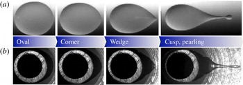
Reference Mulkens, Flagello, Streefkerk and Graeupner2004; Owa & Nagasaka Reference Owa and Nagasaka2008) where a small liquid immersion droplet is held between an optical component and a moving substrate. An example of this similarity is shown in figure 2, where we compare a gravity-driven liquid droplet on an incline (
 $\mathit{Re}\ll 1$
) and an immersion droplet over a moving substrate (
 $\mathit{Re}\sim O(100)$
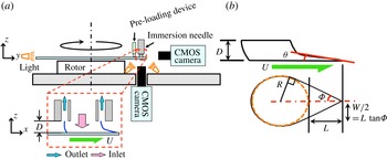
). For the gravity-driven liquid droplet case, the droplet speed is proportional to the inclination angle of the substrate. The immersion droplet speed is determined by the moving substrate (the top of the droplet remains attached to the stationary immersion hood, as shown in figure 3). In this case, the wetting and dewetting speed of contact lines increases to approximately
 $1\ \text{m}\ \text{s}^{-1}$
, i.e.
 $\mathit{Re}\sim O(100)$
for water (Riepen, Evangelista & Donders Reference Riepen, Evangelista and Donders2008; Kim et al.
Reference Kim, Große, Elsinga and Westerweel2011). Regardless of the Reynolds number, the rear part of the droplet evolves from a round shape to a cusp shape when the contact line speed increases. Furthermore, droplet break-up occurs when the half-opening angle
 ${\rm\Phi}$
exceeds 30° (Podgorski, Flesselles & Limat Reference Podgorski, Flesselles and Limat2001; Stone et al.
Reference Stone, Limat, Wilson, Flesselles and Podgorski2002; Riepen et al.
Reference Riepen, Evangelista and Donders2008; see also figure 1 for definition of
 ${\rm\Phi}$
). However, so far no explanation for this similarity has been reported.
Comparison of the transition of the droplet shape in two different geometries and at different Reynolds numbers. (a) Sessile drops on an inclined substrate at
 $\mathit{Re}\ll 1$
. Images taken from Podgorski et al. (Reference Podgorski, Flesselles and Limat2001). (b) A droplet in a model for an immersion lithography machine at
 $\mathit{Re}\sim O(100)$
. In (b), the grey-rounded rim that can be seen inside the droplet is the needle device to supply the flow. Both sets of image are views from the bottom through the transparent glass substrate.

High-speed recording shadowgraphy technique, side and bottom views. (a) Schematic of the experimental set-up. The dashed box shows an enlarged sketch of a liquid immersion droplet over the moving substrate, where
 $D$
is the total height of the droplet and
 $U$
is the velocity of the substrate. The working principle is explained in the text. (b) The geometry and definition of the coordinate systems for the droplet shape, where
 ${\it\theta}$
is the dynamic receding contact angle,
 ${\rm\Phi}$
the half-opening angle,
 $R$
the radius of the main drop, and
 $L$
the length of the elongated tail.

In this study, we perform an experimental and theoretical analysis for the dewetting corner flow problem at
 $\mathit{Re}\,{\it\epsilon}>1$
. First, we observe the shape of a partial dewetting flow structure from the side and bottom view by means of shadowgraphy. From this result, we construct a scaling argument, and then we obtain an empirical model to depict the corner structure of the partial dewetting at
 $\mathit{Re}\,{\it\epsilon}>1$
. This model describes the conical structure by
 ${\it\theta}$
and
 ${\rm\Phi}$
(see the definition of symbols in figures 1 and 3
b). Next, to measure the three-dimensional three-component (referred to as 3D-3C) velocity vectors in a volume, we perform tomographic particle image velocimetry (referred to as tomographic PIV). Through further investigation of the flow pattern, we postulate that the streamlines are straight and nearly parallel in different cross-sectional planes. From the experimental results, we assume that the wall-normal components of the velocity and vorticity are negligible compared to the other components. Based on these results, we present a modified three-dimensional lubrication model for the dewetting corner structure at
 $\mathit{Re}\,{\it\epsilon}>1$
. The model shows that dynamic receding contact angles
 ${\it\theta}$
and half-opening angles
 ${\rm\Phi}$
are correlated with each other. In the model, the modified pressure is introduced that consists of the capillary pressure and the dynamic pressure. When the corner shape is sharper (small
 ${\rm\Phi}$
or high speed
 $U$
), the dynamic pressure effects become important, which is validated by the analytical and experimental results. Furthermore, the model shows that the depth-averaged velocity profile of the corner structure resembles a self-similar flow pattern. We measure the flow pattern for two cases where
 ${\rm\Phi}=40^{\circ }$
and 75°, by means of tomographic PIV. The analytical results are validated and confirmed by the experimental data.
2. Experiments
2.1. High-speed shadowgraphy recording
We perform high-speed shadowgraphy measurements to observe the shape of a partial dewetting droplet over a moving substrate. The schematic of the experimental set-up is shown in figure 3. The liquid droplet is generated by a so-called immersion needle (see the small dashed box of figure 3
a). To maintain a constant volume of the droplet, water is supplied to the centre of the droplet through the inner part of the immersion needle. Then water and air are simultaneously extracted through an annular tube around the inlet. The annular tube of the immersion needle is connected to a constant vacuum pressure of
 $-$
0.5 bar during the measurements (see Kim et al.
Reference Kim, Große, Elsinga and Westerweel2011 for details). The volume of generated drops ranges from approximately 200 to 950 nl by varying the total height (
 $D$
) of the droplet (the gap between the immersion needle and the substrate) in the range
 $200\ {\rm\mu}\text{m}\leqslant D\leqslant 300\ {\rm\mu}\text{m}$
. The droplet has a 1 mm radius (
 $R$
). The liquid droplet is located near the edge of a 12 in. glass wafer, which spins with a constant acceleration up to the critical velocity. Above the critical velocity, the droplet starts to shed satellite droplets at its tail (called ‘pearling’, figure 2). While rotating the wafer, a pre-loading device maintains a constant position of the wafer in the vertical direction. It has been demonstrated earlier that there is no noticeable centrifugal force effect in the flow pattern (Kim et al.
Reference Kim, Große, Elsinga and Westerweel2011).
Three different substrate conditions are used, which lead to typical apparent contact angles
 ${\it\theta}_{0}\approx 89^{\circ }$
, 76°, and 63°, respectively. The substrates have receding contact angles of 81°, 70° and 48° and advancing contact angles of 97°, 82° and 78°, respectively. The hysteresis is measured by the add/remove volume method (De Gennes, Brochard-Wyart & Quéré Reference De Gennes, Brochard-Wyart and Quéré2004). The substrates are coated by ASML Holding NV. To observe the contour of the bottom view a transparent glass wafer (Silicon Valley Microelectronics, Inc.) is used. The working fluid is distilled water with a dynamic viscosity
 ${\it\mu}=10^{-3}\ \text{Pa}\ \text{s}$
, a surface tension
 ${\it\gamma}=72\ \text{mN}\ \text{m}^{-1}$
, and a density
 ${\it\rho}=10^{3}\ \text{kg}\ \text{m}^{-3}$
. The working fluid is continuously circulating to maintain it at a constant room temperature (298 K). The Reynolds number (
 $\mathit{Re}={\it\rho}Uh_{f}/{\it\mu}$
) is much larger than unity, where
 $U$
is the speed of the wafer and
 $h_{f}$
is the droplet tail height. Moreover, the capillary number (
 $\mathit{Ca}={\it\mu}U/{\it\gamma}$
) is approximately 0.014.
The motion is recorded via a high-speed CMOS camera (Photron SA3), with a resolution of
 $1024\ \text{pixel}\times 1024\ \text{pixel}$
and a 12-bit dynamic range and a frame rate of 1000 frames per second (f.p.s.). The camera is equipped with a long-range microscope (Navitar 10X Telecentric Zoom system) giving a resolution of
 $5\ {\rm\mu}\text{m}\ \text{pixel}^{-1}$
for the side view and
 $3\ {\rm\mu}\text{m}\ \text{pixel}^{-1}$
for the bottom view. The wafer substrate is accelerating by
 $1\ \text{m}\ \text{s}^{-2}$
at the position of the droplet during the measurement. Here, the viscous/capillary time scale is approximated as
 ${\it\tau}_{{\it\gamma}}\sim {\it\mu}D/{\it\gamma}\sim 10^{-5}\ (\text{s})$
and this time scale is relatively short compared to the duration of the experimental recording frame rate (order of milliseconds). In this sense, we assume that at each instance the liquid interface is in a quasi-steady state.
Tomographic PIV set-up. (a) Illustration of the PIV set-up, with four PIV cameras mounted on a custom-made microscope at the bottom of the set-up. (b) Cross-sectional schematic of the PIV set-up. The focal length
 $f$
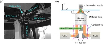
is approximately 31 mm and the inner aperture is approximately 7 mm inside the lens. Particles inside the immersion droplet are volumetrically illuminated at 527 nm wavelength. A diffuser plate is installed between the stereo-microscope and the glass wafer. In the optical box, filters are installed in front of each CCD camera, which only transmit light with wavelengths longer than 535 nm. The laser beam path is also included in the optical box.

2.2. Tomographic PIV
Recently, tomographic PIV has been introduced to measure 3D-3C velocity vectors in both microscopic (Kim et al. Reference Kim, Große, Elsinga and Westerweel2011) and large-scale turbulence problems (Elsinga Reference Elsinga2008). Furthermore, tomographic PIV is able to reconstruct the liquid–air interface, and hence it is possible to apply the velocity measurement to a flow domain with a free surface (Kim, Westerweel & Elsinga Reference Kim, Westerweel and Elsinga2013).
Figure 4 shows the experimental set-up for the volumetric flow measurement. To obtain the three velocity components in a volume we install four CCD cameras (LaVision Imager Intense), each with a resolution of
 $1376\ \text{pixel}\times 1040\ \text{pixel}$
and a 12-bit dynamic range. In this experimental configuration, the equivalent linear dimension of a single pixel in the object domain is
 $4\ {\rm\mu}\text{m}$
. To observe the internal flow field of the partial dewetting flow, the entire volume needs to be accessed with minimal optical distortion due to refraction at the interface. Therefore, the four cameras are mounted on an inverted custom-made microscope, as shown in figure 4. The optical path of each camera is off-axis through a single microscope objective lens with a magnification of 1.5. The offset angle between the optical axes of the cameras is about
 ${\it\alpha}\approx 20^{\circ }$
(see figure 4
b). Volume illumination is achieved using an expanded laser beam with a diameter of 5 mm. An optical diffuser plate is used to avoid speckle effects. As shown in figure 4(b), the custom-made microscope is installed at approximately 30 mm below the wafer surface. The depth-of-field can be estimated by
 ${\rm\Delta}z_{0}\cong 4(1+1/M_{0})^{2}{f^{\#}}^{2}{\it\lambda}$
(e.g. Adrian & Westerweel Reference Adrian and Westerweel2010), where
 ${\rm\Delta}z_{0}$
is the depth-of-field,
 $M_{0}$
the magnification of the lens,
 $f^{\#}$
the
 $f$
-number of the lens and
 ${\it\lambda}$
the wavelength of the light. For the given optical parameters we have
 ${\rm\Delta}z_{0}\approx 120\ {\rm\mu}\text{m}$
. The accuracy of the present experimental system is evaluated in preceding studies (Kim et al.
Reference Kim, Große, Elsinga and Westerweel2011, Reference Kim, Westerweel and Elsinga2013). The error amplitude of the particle displacement that is related to the divergence root-mean-square (r.m.s.) error is between 0.1 and 0.3 pixels. This error is consistent with the typical measurement uncertainty reported for tomographic PIV.
To measure the flow field, the working fluid is seeded with
 $1.28\ {\rm\mu}\text{m}$
tracer particles (Microparticles GmbH, Germany). The particles are labelled with a fluorescent dye (Rhodamine-B) and coated with polyethylene glycol (PEG). This PEG-coating avoids particle coagulation and attachment to the solid surface and to the free surface. Fluorescence is excited by a dual-cavity frequency-doubled pulsed Nd:YLF (
 ${\it\lambda}=527\ \text{nm}$
, Pegasus – New wave research) high-speed laser. The final image density (
 $N_{I}$
) is
 $5.38\times 10^{-1}$
, given by
 $N_{I}\equiv CA_{I}{\rm\Delta}z_{0}/M_{0}^{2}$
, where
 $C$
is the mean number of particles per unit volume
 $(\text{m}^{-3})$
,
 $M_{0}$
the magnification of the lens,
 ${\rm\Delta}z_{0}$
the depth-of-field (m) and
 $A_{I}$
the image interrogation area
 $(\text{m}^{2})$
. The particle image seeding density is 0.034 particles per pixel (p.p.p.) as determined from a typical raw image. The value corresponds to a source density
 $N_{S}\simeq 0.09$
, which is considered to represent a relatively low seeding density (Adrian & Westerweel Reference Adrian and Westerweel2010). This is not adequate for resolving the small scales of the fluid motion close to the moving contact line. In order to effectively increase the density of the reconstructed particle, the 3D intensity volumes are averaged over 25 individually reconstructed volume pairs.
For the multi-camera PIV system, calibration is necessary to correct for the different projections recorded on each of the CCD cameras. A calibration of the image mapping is performed by 3D calibration, and the calibration is corrected by means of volume self-calibration (Wieneke Reference Wieneke2008). After the calibration, the disparity error between the different views is less than 0.05 pixels. The whole pre- and post-processing and calibration procedures are performed by means of a commercial code (Davis 8.05, LaVision GmbH).
For tomographic PIV, the MART (multiplicative algebraic reconstruction technique) algorithm is used with five iterations and with the relaxation parameter
 ${\it\mu}=1$
(Elsinga Reference Elsinga2008). The velocity is obtained by performing 3D cross-correlations of the reconstructed particle distribution in the measurement volume with an interrogation volume of
 $8\ \text{voxel}\times 8\ \text{voxel}\times 8\ \text{voxel}$
with 50 % overlap. The spatial discretization is
 $250\ \text{voxels}\ \text{mm}^{-1}$
. The PIV experimental details are described in detail by Kim et al. (Reference Kim, Große, Elsinga and Westerweel2011, Reference Kim, Westerweel and Elsinga2013).
Evolution of the dynamic receding contact angle
 ${\it\theta}$
where the height of the structure is
 $D=250\ {\rm\mu}\text{m}$
. The elongated liquid droplet tail
 $L$
and the droplet tail height
 $h_{f}$
vary with the speed of the substrate
 $U$
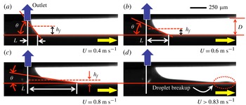
, which is observed from the side by shadowgraphy measurements. The dark arrow indicates the outlet of the immersion needle device.

Evolution of the partial dewetting contact line (i.e. solid curves) by varying the speed of the substrate
 $U$
where the total height of the structure is
 $250\ {\rm\mu}\text{m}$
. Images observed from below by means of shadowgraphy. The dashed-dotted line is the symmetry line of the partial dewetting and
 ${\rm\Phi}$
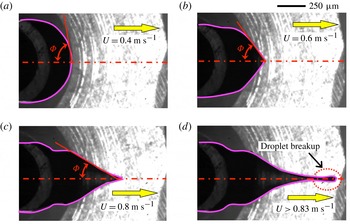
is the half-opening angle. (a) Oval shape, (b) corner shape, (c) corner to cusp shape and (d) droplet breakup.

3. Experimental results and discussion
3.1. Scaling analysis
We observe the shape of the partial dewetting flow from the bottom and side view by means of shadowgraphy. Figures 5 and 6 show examples of the evolution of the partial dewetting by increasing the substrate speed where the substrate is hydrophobic,
 ${\it\theta}_{0}\approx 89^{\circ }$
. At the early stage, the tail structure has a large slope (
 ${\it\theta}$
) and a short tail (
 $L$
) as shown in figure 5(a). Figure 5(b,c) shows that as the substrate speed increases, the tail becomes elongated. When the critical speed is reached, it begins to lose fluid (i.e. droplet breakup), as shown in figure 5(d). Figure 6 shows the shape change of the partial dewetting contact lines in the bottom view, i.e. oval
 $\Rightarrow$
corner
 $\Rightarrow$
cusp
 $\Rightarrow$
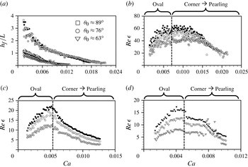
pearling. Furthermore, figure 7(a) shows the evolution of the aspect ratio
 ${\it\epsilon}$
(
 $=h_{f}/L$
) by increasing the substrate speed. The tail length (
 $L$
) and the tail height (
 $h_{f}$
) are defined in figure 5. At the early stage, the aspect ratio is
 ${\it\epsilon}\geqslant 1$
. In particular, in the case of
 ${\it\theta}_{0}\approx 89^{\circ }$
(square symbols in figure 7), the elongated droplet tail is short compared to the tail height (
 $h_{f}$
), which is due to the hydrophobic surface. In the case of hydrophilic substrates, the aspect ratio is smaller than for the hydrophobic one at least in the early stage. However, for all cases, as the substrate speed increases, the droplet shape becomes elongated and thin like a thin-film flow structure, irrespective of the contact angle.
Evolution of (a)
 $h_{f}/L$
and (b–d)
 $\mathit{Re}\,{\it\epsilon}$
with respect to the capillary number
 $\mathit{Ca}$
. The black symbol is for
 $D=300\ {\rm\mu}\text{m}$
, the white
 $D=250\ {\rm\mu}\text{m}$
and grey
 $D=200\ {\rm\mu}\text{m}$
above the different surface conditions, i.e. (b)
 ${\it\theta}_{0}\approx 89^{\circ }$
; (c)
 ${\it\theta}_{0}\approx 76^{\circ }$
; and (d)
 ${\it\theta}_{0}\approx 63^{\circ }$
.

Based on the shadowgraphy results, we perform a scaling analysis for the partial dewetting flow at intermediate Reynolds number in the absolute frame. The following representative scales are taken into consideration:
-
(a) droplet tail height of the liquid drop:
 $50\ {\rm\mu}\text{m}\leqslant h_{f}\leqslant 100\ {\rm\mu}\text{m}$
;
-
(b) length of the liquid drop tail:
$0\leqslant L\leqslant 1\ \text{mm}$
(for
$R=1\ \text{mm}$
); -
(c) substrate speed:
$U\leqslant 1\ \text{m}\ \text{s}^{-1}$
.


Let
 $L$
and
 $h_{f}$
be the characteristic length in the direction of the substrate movement and in the normal direction, respectively. Then, the dimensionless variables are as follows:
 $$\begin{eqnarray}t^{\prime }=t\frac{U}{L},\quad x^{\prime }=\frac{x}{L},\quad z^{\prime }=\frac{z}{h_{f}},\quad u^{\prime }=\frac{u}{U},\quad w^{\prime }=\frac{w}{{\it\epsilon}U},\quad p^{\prime }=\frac{{\it\epsilon}^{2}L}{{\it\mu}U}p,\end{eqnarray}$$
The pressure is normalized by the viscous force and the aspect ratio. Substitution of (3.1) in the momentum equation for
 $u$
yields
 $$\begin{eqnarray}\frac{{\it\rho}U^{2}}{L}\left(\frac{\partial u^{\prime }}{\partial t^{\prime }}+u^{\prime }\frac{\partial u^{\prime }}{\partial x^{\prime }}+w^{\prime }\frac{\partial u^{\prime }}{\partial z^{\prime }}\right)=-\frac{{\it\mu}U}{L^{2}{\it\epsilon}^{2}}\frac{\partial p^{\prime }}{\partial x^{\prime }}+\frac{{\it\mu}U}{L^{2}}\left(\frac{\partial ^{2}u^{\prime }}{\partial {x^{\prime }}^{2}}+\frac{1}{{\it\epsilon}^{2}}\frac{\partial ^{2}u^{\prime }}{\partial {z^{\prime }}^{2}}\right).\end{eqnarray}$$
Given that
 $h_{f}\ll L$
, we have
 $\partial ^{2}u^{\prime }/\partial x^{\prime 2}\ll (1/{\it\epsilon}^{2})(\partial ^{2}u^{\prime }/\partial z^{\prime 2})$
in the viscous terms, and we further divide by
 ${\it\mu}U/L^{2}$
, so that
 $$\begin{eqnarray}\mathit{Re}\,{\it\epsilon}\left(\frac{\partial u^{\prime }}{\partial t^{\prime }}+u^{\prime }\frac{\partial u^{\prime }}{\partial x^{\prime }}+w^{\prime }\frac{\partial u^{\prime }}{\partial z^{\prime }}\right)\cong -\frac{\partial p^{\prime }}{\partial x^{\prime }}+\left(\frac{\partial ^{2}u^{\prime }}{\partial {z^{\prime }}^{2}}\right),\end{eqnarray}$$
where
 $\mathit{Re}$
is the Reynolds number,
 $\mathit{Re}={\it\rho}Uh_{f}/{\it\mu}$
. Here,
 $\mathit{Re}\,{\it\epsilon}$
is larger than unity as shown in figure 7. The inertial forces, i.e. the left-hand side of (3.3), are thus not negligible in comparison with pressure and viscous forces.
In the same manner, in the wall-normal direction, we find
 $$\begin{eqnarray}\frac{{\it\epsilon}{\it\rho}U^{2}}{L}\left(\frac{\partial w^{\prime }}{\partial t^{\prime }}+u^{\prime }\frac{\partial w^{\prime }}{\partial x^{\prime }}+w^{\prime }\frac{\partial w^{\prime }}{\partial z^{\prime }}\right)=-\frac{{\it\mu}U}{{\it\epsilon}^{2}Lh}\frac{\partial p^{\prime }}{\partial z^{\prime }}+\frac{{\it\epsilon}{\it\mu}U}{L^{2}}\left(\frac{\partial ^{2}w^{\prime }}{\partial {x^{\prime }}^{2}}+\frac{1}{{\it\epsilon}^{2}}\frac{\partial ^{2}w^{\prime }}{\partial {z^{\prime }}^{2}}\right),\end{eqnarray}$$
where for the viscous terms,
 $\partial ^{2}w^{\prime }/\partial x^{\prime 2}\ll (1/{\it\epsilon}^{2})(\partial ^{2}w^{\prime }/\partial z^{\prime 2})$
, and we further divide by
 ${\it\epsilon}{\it\mu}U/L^{2}$
, so that
 $$\begin{eqnarray}\mathit{Re}\,{\it\epsilon}^{3}\left(\frac{\partial w^{\prime }}{\partial t^{\prime }}+u^{\prime }\frac{\partial w^{\prime }}{\partial x^{\prime }}+w^{\prime }\frac{\partial w^{\prime }}{\partial z^{\prime }}\right)\cong -\frac{\partial p^{\prime }}{\partial z^{\prime }}+{\it\epsilon}^{2}\left(\frac{\partial ^{2}w^{\prime }}{\partial {z^{\prime }}^{2}}\right).\end{eqnarray}$$
In this result, if the flow structure becomes very thin and long, i.e.
 ${\it\epsilon}\ll 1$
, the pressure in the liquid is independent of the
 $z$
-direction due to negligible inertia and viscous effects, i.e.
 $\mathit{Re}\,{\it\epsilon}^{3}\ll 1$
and
 ${\it\epsilon}^{2}\ll 1$
.
Figure 7 shows that in the observed flow
 $\mathit{Re}\,{\it\epsilon}$
is larger than unity. In particular, at the early stage, when the droplet has an oval shape at the rear part (see figure 6
a),
 $\mathit{Re}\,{\it\epsilon}$
increases with the substrate velocity. Here, the aspect ratio (
 $h_{f}/L$
) is not small enough to neglect the inertial effect, i.e.
 $h_{f}/L>1$
, and therefore the product
 $\mathit{Re}\,{\it\epsilon}$
reaches a maximum of
 $O$
(10) (see figure 7
a). After the droplet assumes the corner shape, the flow structure begins to elongate further and
 $\mathit{Re}\,{\it\epsilon}$
decreases. However, it remains relatively large, i.e.
 $\mathit{Re}\,{\it\epsilon}>1$
.
Based on a further analysis of this scaling argument, we obtain a result that describes the relation between
 ${\it\theta}$
and
 ${\rm\Phi}$
. In order to eliminate the pressure terms, we take the curl of (3.3) and (3.5), and we obtain
 $$\begin{eqnarray}\displaystyle & & \displaystyle (\mathit{Re}\,{\it\epsilon})\frac{\partial }{\partial z^{\prime }}\left[\left(\frac{\partial u^{\prime }}{\partial t^{\prime }}+u^{\prime }\frac{\partial u^{\prime }}{\partial x^{\prime }}+w^{\prime }\frac{\partial u^{\prime }}{\partial z^{\prime }}\right)\right]-(\mathit{Re}\,{\it\epsilon}^{3})\frac{\partial }{\partial x^{\prime }}\left[\left(\frac{\partial w^{\prime }}{\partial t^{\prime }}+u^{\prime }\frac{\partial w^{\prime }}{\partial x^{\prime }}+w^{\prime }\frac{\partial w^{\prime }}{\partial z^{\prime }}\right)\right]\nonumber\\ \displaystyle & & \displaystyle \quad \cong \left[\frac{\partial }{\partial z^{\prime }}\left({\it\epsilon}^{2}\frac{\partial ^{2}u^{\prime }}{\partial x^{\prime 2}}+\frac{\partial ^{2}u^{\prime }}{\partial z^{\prime 2}}\right)\right]-{\it\epsilon}^{2}\left[\frac{\partial }{\partial x^{\prime }}\left({\it\epsilon}^{2}\frac{\partial ^{2}w^{\prime }}{\partial x^{\prime 2}}+\frac{\partial ^{2}w^{\prime }}{\partial z^{\prime 2}}\right)\right],\end{eqnarray}$$
where
 $(\mathit{Re}\,{\it\epsilon})\gg (\mathit{Re}\,{\it\epsilon}^{3})$
on the left-hand side and
 $1\gg {\it\epsilon}^{2}$
on the right-hand side. The result shows that the inertial forces are balanced with the viscous forces:
 $$\begin{eqnarray}\overbrace{\mathit{Re}\,{\it\epsilon}\left(=\frac{{\it\rho}UL}{{\it\mu}}\ {\it\epsilon}^{2}\right)}^{\text{inertia}}\sim \overbrace{1}^{\text{viscous}}.\end{eqnarray}$$
According to figure 3(b), the elongated tail length
 $L$
can be approximated using the half-opening angle
 ${\rm\Phi}$
(see this definition in the inset of figure 8) and the radius
 $R$
of the liquid droplet,
 $$\begin{eqnarray}L\approx R\left(\sin {\rm\Phi}^{-1}-1\right)\!.\end{eqnarray}$$
Furthermore, if we assume that the aspect ratio (
 ${\it\epsilon}$
) can be written as
 $\tan {\it\theta}$
, then (3.7) becomes
 $$\begin{eqnarray}L\approx R\left(\frac{1}{\sin {\rm\Phi}}-1\right)\sim \frac{{\it\mu}}{{\it\rho}U\tan ^{2}{\it\theta}}.\end{eqnarray}$$
This results in the following expression:
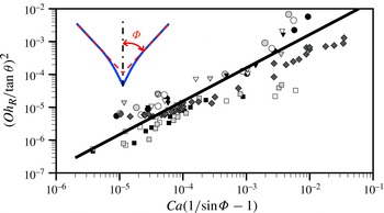
 $$\begin{eqnarray}\left(\frac{Oh_{R}}{\tan {\it\theta}}\right)^{2}\cong \left[\mathit{Ca}\left(\frac{1}{\sin {\rm\Phi}}-1\right)\right],\end{eqnarray}$$
where
 ${\it\theta}$
is the dynamic receding contact angle and
 ${\rm\Phi}$
is the half-opening angle. The Ohnesorge number
 $Oh_{R}$
is
 ${\it\mu}/\sqrt{{\it\rho}{\it\gamma}R}$
where
 $R$
is the radius of the immersion droplet. This dimensionless number describes the ratio of viscous forces to inertial and surface tension forces. We evaluate the validity of (3.10) experimentally. The dynamic receding contact angle
 ${\it\theta}$
is determined from a fit to the liquid interface data within a distance of
 $50\ {\rm\mu}\text{m}$
from the corner tip of the droplet. We measure the half-opening angle
 ${\rm\Phi}$
as shown in the inset of figure 8. For
 ${\rm\Phi}$
and
 ${\it\theta}$
, the measurement error is approximately
 $\pm 2^{\circ }$
. This result confirms that dynamic receding contact angles and half-opening angles are correlated with each other according to the relation (3.10).
 $(Oh_{R}/\!\tan {\it\theta})^{2}$
versus
 $\mathit{Ca}(1/\!\sin {\rm\Phi}-1)$
for three different substrates where: ○,
 ${\it\theta}_{0}\approx 76^{\circ }$
; ▿,
 ${\it\theta}_{0}\approx 63^{\circ }$
; ▫, ♢,
 ${\it\theta}_{0}\approx 89^{\circ }$
. The black symbol (
 $R=1\ \text{mm}$
) represents data for
 $D=300\ {\rm\mu}\text{m}$
; the white (
 $R=1\ \text{mm}$
) and dark grey (
 $R=0.5\ \text{mm}$
),
 $D=250\ {\rm\mu}\text{m}$
; the grey (
 $R=1\ \text{mm}$
),
 $D=200\ {\rm\mu}\text{m}$
. The solid line represents a linear fit to the combined measurement results.

Full 3D-3C velocity distribution and streamlines in the liquid immersion droplet on the moving substrate (
 $U=0.7\ \text{m}\ \text{s}^{-1}$
) at
 $\mathit{Re}\,{\it\epsilon}=4.1$
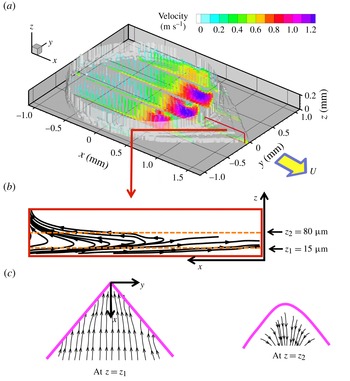
. (a) 3D-3C velocity components at five arbitrary cross-sectional planes, where the white surface contour indicates the shape of the liquid immersion droplet on the moving substrate. (b) Streamlines (box) at the cross-sectional plane (
 $y=-0.04\ \text{mm}$
). (c) In-plane streamlines at
 $z_{1}=15\ {\rm\mu}\text{m}$
. (d) In-plane streamlines at
 $z_{2}=80\ {\rm\mu}\text{m}$
.

3.2. Internal flow pattern
We obtain the 3D-3C flow field inside the liquid immersion droplet on the moving substrate at
 $U=0.7\ \text{m}\ \text{s}^{-1}$
by means of tomographic PIV, as shown in figure 9(a). The obtained flow field contains
 $147\times 132\times 15$
velocity vectors for the whole droplet. The half-opening angle is
 ${\rm\Phi}=40^{\circ }$
. The external shape (i.e. the liquid–air interface) of the liquid immersion droplet is indicated by the white contour, i.e. where the velocity magnitude is zero. This was determined from the reconstructed 3D tomographic intensity data. We only plot velocity vector profiles at five arbitrary cross-sectional planes in figure 9(a). The colour of the vectors represents the velocity magnitude. The flow field is mainly driven by the moving substrate and the boundary conditions of the immersion needle (see figure 3
a). Near the rear part of the outlet (
 $x=0.75\ \text{mm}$
), we observe a strong extraction flow field. Given the current experimental set-up, where the internal flow pattern is observed from below, it is difficult to obtain the velocity vectors at the advancing part where the contact angle is large. At the advancing part, a relatively small amount of reliable data was obtained, and the liquid–gas interface shape is therefore difficult to reconstruct. However, in this study, we focus on the dewetting corner. Figure 9(b) shows the streamline results at an arbitrary cross-sectional plane (
 $y=-0.04\ \text{mm}$
) (see more visualizations at different cross-sectional planes in figure 16 of appendix A. Two in-plane streamline plots at different
 $z$
positions are shown in figure 9(c,d), where the thick solid lines indicate the contact lines. Note that streamlines at cross-sectional planes are more or less parallel and straight.
4. Theoretical model
4.1. Modified three-dimensional lubrication model for the dewetting corner
This section is devoted to a presentation of a three-dimensional lubrication model for the corner structure at
 $\mathit{Re}\,{\it\epsilon}>1$
. The model problem describes the rear part of the partial dewetting, as shown in figure 10(a). The flow is governed by the incompressible Navier–Stokes equations and continuity equation,
 $$\begin{eqnarray}\boldsymbol{{\rm\nabla}}\boldsymbol{\cdot }\boldsymbol{u}=0,\quad {\it\rho}\left[\frac{\partial \boldsymbol{u}}{\partial t}+(\boldsymbol{u}\boldsymbol{\cdot }\boldsymbol{{\rm\nabla}})\boldsymbol{u}\right]+\boldsymbol{{\rm\nabla}}p={\it\mu}{\rm\nabla}^{2}\boldsymbol{u},\end{eqnarray}$$
where
 $\boldsymbol{u}=(u,v,w)$
and assuming that the gravity does not play a role in this problem. We use the vector identities
 $(\boldsymbol{u}\boldsymbol{\cdot }\boldsymbol{{\rm\nabla}})\boldsymbol{u}\equiv \boldsymbol{{\rm\nabla}}\left(\boldsymbol{u}/2\boldsymbol{\cdot }\boldsymbol{u}\right)-\boldsymbol{u}\times {\bf\omega}$
and
 ${\rm\nabla}^{2}\boldsymbol{u}\equiv \boldsymbol{{\rm\nabla}}(\boldsymbol{{\rm\nabla}}\boldsymbol{\cdot }\boldsymbol{u})-\boldsymbol{{\rm\nabla}}\times (\boldsymbol{{\rm\nabla}}\times \boldsymbol{u})$
where
 ${\bf\omega}=({\it\omega}_{x},{\it\omega}_{y},{\it\omega}_{z})=\boldsymbol{{\rm\nabla}}\times \boldsymbol{u}$
and
 $\boldsymbol{{\rm\nabla}}\equiv (\partial /\partial x,\partial /\partial y,\partial /\partial z)$
.
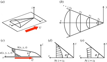
(a) Sketch of the partial dewetting contact line shape observed for the substrate moving with a certain speed showing the droplet curvature. (b) Local cross-sectional plane at each
 $x$
-position. (c) The usual cross-sectional flow pattern near a contact line at
 $y=0$
. (d) Example of the planar flow field at
 $z=z_{1}$
; (e) another example at
 $z=z_{2}$
. Here,
 $z_{1}$
is at a plane where the flow is towards the tip of the tail and
 $z_{2}$
is at a plane where the flow is away from the tail, where
 $z_{2}>z_{1}$
.

Let us first consider here a scaling analysis for the dewetting flow problem at intermediate Reynolds numbers, which assists in deriving the extended lubrication model. This situation is representative of the flow in a liquid drop applied to a model of a liquid-immersion lithography machine, as sketched in the dashed box of figure 3(a). The device generates a constant liquid volume over either a stationary or a moving surface. For the model problem, we focus on the tail part of the dewetting problem. If the substrate is moving with a speed
 $U$
, then the dewetting flow structure resembles a finite thin and long conical shape, as shown in figure 10(a). For the scaling argument, we consider the following relevant length scales:
 $x\sim L,y\sim W$
and
 $z\sim h_{f}$
. On increasing the substrate speed to
 $1\ \text{m}\ \text{s}^{-1}$
, typical length scales are
 $L\sim 10^{-3}\ \text{m}$
,
 $W\sim 10^{-4}\ \text{m}$
, and
 $h_{f}\sim 10^{-5}\ \text{m}$
, so
 $(h_{f}/W)^{2}$
and
 $(h_{f}/L)^{2}\ll 1$
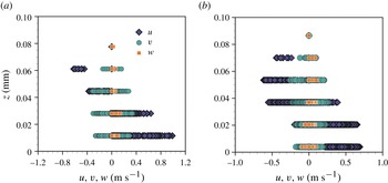
. Furthermore, the streamwise and spanwise velocities in the corner structure are dominant compared to the wall-normal component,
 $w\ll u,v$
, as shown in figure 11 (see also Kim et al.
Reference Kim, Große, Elsinga and Westerweel2011).
Comparison of the three velocity components of the dewetting corner flow along the droplet height: (a)
 ${\rm\Phi}=75^{\circ }$
and (b)
 ${\rm\Phi}=40^{\circ }$
.

In § 3.2, we presented the internal flow pattern in figure 9. At the dewetting rear part of the droplet, the flow streamlines are approximately parallel and straight between the free surface and the moving substrate, as shown in figure 9(b). In this case, we can assume that the cross-sectional flow structure is as in figure 10(c–e), i.e. the streamlines are straight and nearly parallel. This assumption implies
 $w\cong 0$
compared to (
 $u,v$
). In this case, the pressure is independent of
 $z$
(see (3.5)). The static pressure is determined by the spanwise droplet curvature
 $p(x,y)=-{\it\gamma}{\rm\Delta}h$
from the Young–Laplace equation (Snoeijer et al.
Reference Snoeijer, Rio, Le Grand and Limat2005), where the flow is assumed to be incompressible,
 $h$
is the interface height, and
 ${\rm\Delta}\equiv \partial ^{2}/\partial x^{2}+\partial ^{2}/\partial y^{2}$
.
By scaling arguments, the viscous terms reduce to
 ${\it\mu}(\partial ^{2}\boldsymbol{u}/\partial z^{2})$
where
 $\boldsymbol{u}=(u,v,0)$
. For an incompressible flow, the continuity equation is satisfied, so that
 $\boldsymbol{{\rm\nabla}}\boldsymbol{\cdot }\boldsymbol{u}=0$
. Owing to this result, the viscous terms are reduced to
 $-\boldsymbol{{\rm\nabla}}\times (\boldsymbol{{\rm\nabla}}\times \boldsymbol{u})$
. This must be equal to
 ${\it\mu}(\partial ^{2}\boldsymbol{u}/\partial z^{2})$
by the scaling argument. To satisfy this condition, the
 $z$
component of the vorticity
 ${\it\omega}_{z}$
must be negligible compared to the other vorticity components
 ${\it\omega}_{x}$
and
 ${\it\omega}_{y}$
(except for the region very close to the liquid interfaces), which is validated by the experimental results (see figure 9).
Based on these assumptions (
 $w=0$
and
 ${\it\omega}_{z}=0$
), the modified pressure is defined as
 $p^{\ast }=-{\it\gamma}{\rm\Delta}h+{\it\rho}q^{2}/2$
where
 $q=\Vert \boldsymbol{u}\Vert$
is the magnitude of the local fluid velocity. For the steady case the following modified governing equation, including dynamic pressure effects, can be formulated:
 $$\begin{eqnarray}-\boldsymbol{{\rm\nabla}}p^{\ast }+{\it\mu}\frac{\text{d}^{2}\boldsymbol{u}}{\text{d}z^{2}}\cong \mathbf{0},\end{eqnarray}$$
where
 ${\it\mu}$
is the dynamic viscosity. As a result, the viscous forces are balanced by the capillary pressure (
 $-{\it\gamma}{\rm\Delta}h$
) and the dynamic pressure (
 ${\it\rho}q^{2}/2$
).
Let us consider a capillary length in a dynamic situation. Normally, the capillary length can be estimated from a force balance between the Laplace pressure
 ${\it\gamma}{\it\kappa}$
and the hydrostatic pressure
 ${\it\rho}g{\it\kappa}^{-1}$
, i.e.
 ${\it\kappa}^{-1}=\sqrt{{\it\gamma}/{\it\rho}g}$
. In equilibrium, the capillary length for water is normally approximately 3 mm, with a surface tension
 ${\it\gamma}$
of
 $72\ \text{mN}\ \text{m}^{-1}$
, a density
 ${\it\rho}$
of
 $10^{3}\ \text{kg}\ \text{m}^{-3}$
, and a gravitational acceleration
 $g=9.8\ \text{m}\ \text{s}^{-2}$
. However, if gravity is negligible or the Laplace pressure is balanced by another force, e.g. an inertial force, the capillary length can be expressed as
 ${\it\kappa}^{-1}\cong \sqrt{2{\it\gamma}\ell /{\it\rho}q^{2}}$
where
 $\ell$
is characteristic length scale and
 $q$
is the speed of the droplet (Biance et al.
Reference Biance, Chevy, Clanet, Lagubeau and Quéré2006; Reyssat, Pardo & Quéré Reference Reyssat, Pardo and Quéré2009). In this situation, we can neglect gravity, and the Laplace pressure is balanced by
 ${\it\rho}q^{2}({\it\kappa}^{-1}/\ell )/2$
, which is in terms of the dynamic pressure.
Here, we adopt this dynamic capillary length scale. In the dynamic situation of dewetting, the local free-surface curvature (i.e. the inverse of the capillary length) varies with the
 $x$
-position as shown in figure 10(b). The curvature becomes large as one approaches the corner tip at
 $(x,y)=(0,0)\ \text{mm}$
. To estimate the local curvature profile, we suggest that the local capillary length is described by
 $$\begin{eqnarray}{\it\kappa}^{-1}\equiv ({\rm\Delta}h)^{-1}\cong \left(\frac{2h{\it\gamma}}{{\it\rho}q^{2}{\it\epsilon}_{x}^{2}}\right)^{1/2},\end{eqnarray}$$
where
 $\ell$
is expressed as
 $h/{\it\epsilon}_{x}^{2}$
, where
 $h$
is the local height of the partial dewetting flow, which is function of
 $x$
, and
 ${\it\epsilon}_{x}$
is the local aspect ratio
 $h/x$
. By this relation, we assume that the dynamic pressure gradient effect is dominant in the droplet tail length direction compared to the depth direction. As a consequence, the dynamic pressure can be expressed in terms of the dynamic capillary length,
 ${\it\rho}q^{2}/2\cong {\it\gamma}\ell ({\rm\Delta}h)^{2}$
.
To obtain the velocity profile, the boundary conditions are taken as the no-slip boundary condition at the wall and no tangential stress at the free surface. The velocity profile is then obtained by substituting the expression for the dynamic capillary length, (4.3), into the term describing the dynamic pressure in (4.2); integrating the equation in the
 $z$
-direction then gives
 $$\begin{eqnarray}\boldsymbol{u}=\frac{1}{2{\it\mu}}\boldsymbol{{\rm\nabla}}\left(-{\it\gamma}{\rm\Delta}h+\frac{{\it\gamma}x^{2}}{h}({\rm\Delta}h)^{2}\right)\left(z^{2}-2hz\right)-\boldsymbol{U},\end{eqnarray}$$
where
 $\boldsymbol{U}$
is the substrate velocity and
 $h(x,y)$
is the free-surface profile. The velocity profile is a combination of Poiseuille flow and Couette flow.
The modified total pressure consists of the capillary pressure and the dynamic pressure, so that (4.2) can be expressed as
 $$\begin{eqnarray}\boldsymbol{{\rm\nabla}}\biggl(\underbrace{-{\it\gamma}{\rm\Delta}h}_{\text{capillary pressure}}+\overbrace{\frac{{\it\gamma}x^{2}}{h}({\rm\Delta}h)^{2}}^{\text{dynamic pressure}}\biggr)-\underbrace{\frac{3{\it\mu}\boldsymbol{U}}{h^{2}}}_{\text{viscous force}}=\mathbf{0},\end{eqnarray}$$
where
 $\boldsymbol{U}$
is the two-dimensional depth-averaged velocity profile in a coordinate system attached to the moving substrate,
 $\boldsymbol{U}(x,y)=(1/h)\int _{0}^{h}\text{d}z\,\boldsymbol{u}$
. If the surface tension is constant, then (4.5) can be re-written as
 $$\begin{eqnarray}\boldsymbol{{\rm\nabla}}{\rm\Delta}h-\frac{3{\it\mu}\boldsymbol{U}}{{\it\gamma}h^{2}}\biggl[1+\overbrace{\frac{{\it\gamma}h^{2}}{3{\it\mu}\boldsymbol{U}}\boldsymbol{{\rm\nabla}}\left(\frac{x^{2}}{h}({\rm\Delta}h)^{2}\right)}^{\text{dynamic pressure effect}}\biggr]=\mathbf{0}.\end{eqnarray}$$
This result is similar to the classical lubrication equation, but now accounting for the dynamic pressure. For a sliding droplet in the Stokes regime, the lubrication model is
 $\boldsymbol{{\rm\nabla}}{\rm\Delta}h=3{\it\mu}\boldsymbol{U}/{\it\gamma}h^{2}$
, which is the force balance between the static capillary force and the viscous force (Limat & Stone Reference Limat and Stone2004). The conventional lubrication theory model can be modified for the dynamic pressure, provided that the flow pattern at the corner has straight and nearly parallel streamlines.
4.2. Modified interface equation
$H({\it\zeta})$
for dewetting corner

Stone et al. (Reference Stone, Limat, Wilson, Flesselles and Podgorski2002) and Limat & Stone (Reference Limat and Stone2004) introduced the interface equation
 $H(y/x)$
to describe the three-dimensional corner structure using a similarity solution
 $h(x,y)=\mathit{Ca}^{1/3}xH(y/x)$
where
 $\mathit{Ca}={\it\mu}U/{\it\gamma}$
is the capillary number. The final equation is a nonlinear fourth-order ordinary differential equation (ODE) that was validated using experimental data. Although it is limited to the Stokes flow regime and small receding contact angles, the model is useful for understanding the shape transition mechanism of partial dewetting contact lines.
In this section, we extend the lubrication model to
 $\mathit{Re}\,{\it\epsilon}>1$
for the case of a flow pattern with straight and nearly parallel streamlines. To obtain the interface equation
 $h(x,y)$
, (4.5) should satisfy the depth-averaged mass conservation, and if the interface is considered in a reference frame moving with the droplet, then
 $$\begin{eqnarray}\frac{\partial h}{\partial t}+\boldsymbol{{\rm\nabla}}\boldsymbol{\cdot }(h\boldsymbol{U})=0,\end{eqnarray}$$
where
 $h(x-Ut,y)$
describes the partial dewetting interface in the moving reference frame. Then, we substitute
 $\boldsymbol{U}$
from (4.5) into (4.7) and obtain a result for the interface shape:
 $$\begin{eqnarray}3\mathit{Ca}\frac{\partial h}{\partial x}=\boldsymbol{{\rm\nabla}}\boldsymbol{\cdot }\left[h^{3}\boldsymbol{{\rm\nabla}}\left({\rm\Delta}h-\frac{x^{2}}{h}\left({\rm\Delta}h\right)^{2}\right)\right].\end{eqnarray}$$
This is the modified three-dimensional corner structure equation at
 $\mathit{Re}\,{\it\epsilon}>1$
. Then, if we adopt the similarity Ansatz
 $h(x,y)=\mathit{Ca}^{1/3}xH({\it\zeta})$
where
 ${\it\zeta}=y/x$
(Limat & Stone Reference Limat and Stone2004), the result yields
 $$\begin{eqnarray}\displaystyle 3(H-{\it\zeta}H_{{\it\zeta}}) & = & \displaystyle (1+{\it\zeta}^{2})^{2}(H^{3}H_{{\it\zeta}{\it\zeta}{\it\zeta}})_{{\it\zeta}}+3{\it\zeta}(1+{\it\zeta}^{2})(H^{3}H_{{\it\zeta}{\it\zeta}})_{{\it\zeta}}+2{\it\zeta}(1+{\it\zeta}^{2})H^{3}H_{{\it\zeta}{\it\zeta}{\it\zeta}}\nonumber\\ \displaystyle & & \displaystyle +\,(1+3{\it\zeta}^{2})H^{3}H_{{\it\zeta}{\it\zeta}}-\left[(1+{\it\zeta}^{2})^{3}(-HH_{{\it\zeta}}H_{{\it\zeta}{\it\zeta}}^{2}+2H^{2}H_{{\it\zeta}{\it\zeta}}H_{{\it\zeta}{\it\zeta}{\it\zeta}})_{{\it\zeta}}\right.\nonumber\\ \displaystyle & & \displaystyle +\,4{\it\zeta}(1+{\it\zeta}^{2})^{2}(4HH_{{\it\zeta}{\it\zeta}{\it\zeta}}+H_{{\it\zeta}}H_{{\it\zeta}{\it\zeta}})HH_{{\it\zeta}{\it\zeta}}+2{\it\zeta}(1+\,{\it\zeta}^{2})^{2} (HH_{{\it\zeta}{\it\zeta}{\it\zeta}}\nonumber\\ \displaystyle & & \displaystyle \left.+\,H_{{\it\zeta}}H_{{\it\zeta}{\it\zeta}})HH_{{\it\zeta}{\it\zeta}}+3(1+5{\it\zeta}^{2})(1+{\it\zeta}^{2})H^{2}H_{{\it\zeta}{\it\zeta}}^{2}\!\right],\end{eqnarray}$$
where
 $H({\it\zeta})$
is independent of the capillary number and the Reynolds number. The derivatives of
 $H({\it\zeta})$
with respect to
 ${\it\zeta}$
are written
 $H_{{\it\zeta}}$
.
The partial dewetting corner structure
 $H({\it\zeta})$
is described by a fourth-order ODE. To solve this equation, we apply two boundary conditions,
 $H_{{\it\zeta}}(0)=H_{{\it\zeta}{\it\zeta}{\it\zeta}}(0)=0$
, because of the symmetry. Further, there are two independent parameters
 $H(0)=H_{0}$
and
 $H_{{\it\zeta}{\it\zeta}}(0)$
. However, each
 $H_{0}$
has several
 $H_{{\it\zeta}{\it\zeta}}(0)$
solutions (Limat & Stone Reference Limat and Stone2004). To choose the proper value for
 $H_{{\it\zeta}{\it\zeta}}(0)$
, Limat & Stone (Reference Limat and Stone2004) suggested that when the curvature
 $H({\it\zeta})$
obeys mass conservation, there is a unique
 $H_{{\it\zeta}{\it\zeta}}(0)$
for each
 $H_{0}$
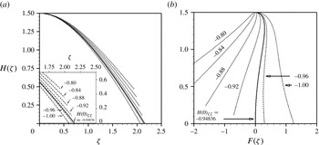
. As shown in figure 12, for (4.9), each
 $H_{0}$
also has several
 $H_{{\it\zeta}{\it\zeta}}(0)$
. To find the matching solution, the
 $x$
-flux integrated over a cross-sectional plane must be zero. This statement can be expressed as
 $$\begin{eqnarray}F({\it\zeta})=\int _{0}^{{\it\zeta}}\left[H^{3}\left(\left[{\it\zeta}[1+{\it\zeta}^{2}]H_{{\it\zeta}{\it\zeta}}-\frac{H_{{\it\zeta}{\it\zeta}}^{2}}{H}\left[1+{\it\zeta}^{2}\right]^{2}{\it\zeta}\right]_{{\it\zeta}}+\frac{3}{H^{2}}\right)\right]\text{d}{\it\zeta}=0,\end{eqnarray}$$
where the flux is integrated between
 $y=-{\it\zeta}x$
and
 $y={\it\zeta}x$
. This integrated equation can be derived in the same manner as mentioned in the literature (Limat & Stone Reference Limat and Stone2004). As shown in figure 12(b), each
 $H(0)$
has a unique
 $H_{{\it\zeta}{\it\zeta}}(0)$
solution that satisfies
 $F({\it\zeta})\rightarrow 0$
and
 $H({\it\zeta})\rightarrow 0$
. In this problem, the solution is
 $H_{{\it\zeta}{\it\zeta}}(0)=-0.94836$
for
 $H_{0}=1.5$
. To obtain the proper
 $H_{{\it\zeta}{\it\zeta}}(0)$
, we use the shooting method with a fourth-order Runge–Kutta method.
Solutions of the interface
 $H({\it\zeta})$
equation. (a)
 $H({\it\zeta})$
versus
 ${\it\zeta}$
; different solutions of (4.9) with
 $H(0)=1.5$
and different initial
 $H_{{\it\zeta}{\it\zeta}}(0)$
. The solid line is the exact solution to satisfy (4.10). (b)
 $H({\it\zeta})$
versus
 $F({\it\zeta})$
shows that there is only one pair
 $H(0)$
and
 $H_{{\it\zeta}{\it\zeta}}(0)$
that satisfies the mass conservation.

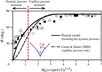
We numerically solve (4.9) and plot the results as the solid line in figure 13, which is the relationship between the half-opening angle
 ${\rm\Phi}$
and
 $H_{0}\ (=\mathit{Ca}^{-1/3}\tan {\it\theta})$
. This prediction is validated using experimental data. We measure two angles,
 ${\rm\Phi}$
and
 ${\it\theta}$
, and then plot all measurement results of the partial dewetting problem in figure 13. The dashed-dotted line is the numerical result for the gravity-driven droplet on an inclined plane, which was investigated by Limat & Stone (Reference Limat and Stone2004) and Snoeijer et al. (Reference Snoeijer, Rio, Le Grand and Limat2005). They used the classical lubrication approximation, ignoring convective acceleration (inertial) terms. Our model (the solid line) provides a better prediction for the relation between
 ${\rm\Phi}$
and
 $H_{0}$
as the half-opening angle becomes smaller, i.e. at large substrate speeds.
Comparison of numerical results for the relation between half-opening angle
 ${\rm\Phi}$
and
 $\tan {\it\theta}/\mathit{Ca}^{1/3}$
. The solid line has been obtained numerically from (4.9) and (4.10). The dashed-dotted line is the numerical result of Limat & Stone (Reference Limat and Stone2004) that is based on the Stokes flow regime. The symbols are experimental data for this partial dewetting flow problem for three different surface conditions (see figure 7
a) and colours indicate the different drop volumes: black, results for
 $D=300\ {\rm\mu}\text{m}$
; white,
 $D=250\ {\rm\mu}\text{m}$
; grey,
 $D=200\ {\rm\mu}\text{m}$
where the radius of droplets is
 $R=1\ \text{mm}$
.

Limat & Stone (Reference Limat and Stone2004) assumed that the cross-sectional plane of the conical dewetting shape can be approximated by a parabolic shape, i.e.
 $h(x,y)\approx H_{0}\ \mathit{Ca}^{1/3}x[1-y^{2}/(x^{2}\tan ^{2}{\it\phi})]$
. We use this assumption to describe the shape of the partial dewetting flow at intermediate Reynolds numbers. From (4.5), we obtain the approximate analytical solution
 $$\begin{eqnarray}\tan ^{3}{\it\theta}\approx \overbrace{{\textstyle \frac{3}{2}}\mathit{Ca}\tan ^{2}{\rm\Phi}}^{\text{capillary pressure}}+\overbrace{{\textstyle \frac{3}{4}}\mathit{Ca}\tan ^{4}{\rm\Phi}}^{\text{dynamic pressure}}.\end{eqnarray}$$
Figure 13 shows that when
 ${\rm\Phi}<60^{\circ }$
,
 $(3/4)\mathit{Ca}\tan ^{4}{\rm\Phi}$
becomes the dominant term. In contrast, when the angle
 ${\rm\Phi}$
is larger than approximately 60°, the term
 $\frac{3}{2}\mathit{Ca}\tan ^{2}{\rm\Phi}$
is dominant. Hence, we can postulate that there are two approximate solutions to describe the relationship between
 ${\it\theta}$
and
 ${\rm\Phi}$
. In the present partial dewetting flow at intermediate Reynolds numbers, the dynamic pressure effects become more important when the half-opening angle gets smaller.
4.3. Self-similar flow pattern at
$\mathit{Re}\,{\it\epsilon}>1$

Based on the present lubrication model, we can obtain the two-dimensional mean velocity profile in the corner structure. From (4.5), we express the two-dimensional mean velocity profile in a coordinate system attached to the moving substrate:
 $$\begin{eqnarray}\boldsymbol{U}(x,y)=\frac{{\it\gamma}h^{2}}{3{\it\mu}}\left(\boldsymbol{{\rm\nabla}}{\rm\Delta}h-\boldsymbol{{\rm\nabla}}\left[\frac{x^{2}}{h}({\rm\Delta}h)^{2}\right]\right).\end{eqnarray}$$
By the similarity Ansatz
 $h(x,y)=\mathit{Ca}^{1/3}xH({\it\zeta})$
, we can obtain the velocity profile in a polar coordinate system (
 $r,{\it\phi}$
):
 $$\begin{eqnarray}\left.\begin{array}{@{}lll@{}}\displaystyle U_{r} & = & \overbrace{-\frac{U}{3}\frac{H^{2}H_{{\it\zeta}{\it\zeta}}}{\cos {\it\phi}}}^{\text{capillary pressure}}+\overbrace{\frac{U}{3}\frac{HH_{{\it\zeta}{\it\zeta}}^{2}}{\cos ^{3}{\it\phi}}}^{\text{dynamic pressure}},\\ \displaystyle U_{{\it\phi}} & = & \underbrace{\frac{U}{3}\frac{H^{2}}{\cos ^{3}{\it\phi}}\left(H_{{\it\zeta}{\it\zeta}{\it\zeta}}+\frac{3}{2}H_{{\it\zeta}{\it\zeta}}\sin 2{\it\phi}\right)}_{\text{capillary pressure}}\\ & & \displaystyle -\,\underbrace{\frac{U}{3}\frac{HH_{{\it\zeta}{\it\zeta}}}{\cos ^{5}{\it\phi}}\left(-\frac{H_{{\it\zeta}}H_{{\it\zeta}{\it\zeta}}}{H}+2H_{{\it\zeta}{\it\zeta}{\it\zeta}}+\frac{5}{2}H_{{\it\zeta}{\it\zeta}}\sin 2{\it\phi}\right)}_{\text{dynamic pressure}},\end{array}\right\}\end{eqnarray}$$
where
 $x=r\cos {\it\phi}$
and
 $y=r\sin {\it\phi}$
. We use the (
 $r,{\it\phi}$
) coordinates to indicate the local position (
 $r$
) from the corner tip and the angle (
 ${\it\phi}$
) within the corner shape, where
 $-{\rm\Phi}\leqslant {\it\phi}\leqslant {\rm\Phi}$
. Derivatives of
 $H({\it\zeta})$
with respect to
 ${\it\zeta}$
are written
 $H_{{\it\zeta}}$
(see the solution details in appendix B).
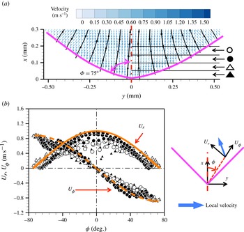
Comparison of tomographic PIV results and the analytical solution where the half-opening angle is
 ${\rm\Phi}=75^{\circ }$
. (a) The depth-averaged velocity vectors (colours) and streamlines (black) of the partial dewetting flow where the vectors are the apparent velocities in the moving coordinates frame. (b) Self-similar flow pattern:
 $U_{r}$
(solid) and
 $U_{{\it\phi}}$
(dashed) indicate analytical results for the radial and angular velocity components, respectively. The corresponding experimental data are shown by symbols, defined in (a), where the data have been divided into slices of
 ${\rm\Delta}x=50\ {\rm\mu}\text{m}$
distance each from the corner of the drop. The two velocity components are decomposed as shown on the right of (b). The centre of the droplet is the red dashed-dot line and the purple solid lines indicate the contact lines.

To validate this result, we compare this solution with the measurement results obtained with tomographic PIV. We measure the volumetric flow field in the rear part of two partial dewetting droplets where the half-opening angles are
 ${\rm\Phi}=40^{\circ }$
and 75°. The experiments are performed in the same manner as in a previous study (Kim et al.
Reference Kim, Große, Elsinga and Westerweel2011). The obtained flow field contains
 $179\times 133\times 15$
velocity vectors for
 ${\rm\Phi}=75^{\circ }$
and
 $147\times 132\times 15$
velocity vectors for
 ${\rm\Phi}=40^{\circ }$
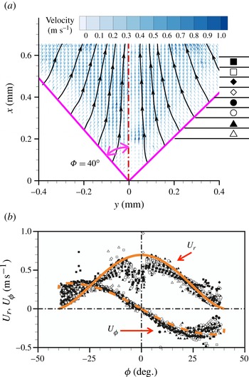
. Figures 14 and 15 show the depth-averaged velocity vector field at the dewetting corner region for
 ${\rm\Phi}=75^{\circ }$
and
 ${\rm\Phi}=40^{\circ }$
, respectively. In figures 14(a) and 15(a), each symbol indicates a different slice with respect to the corner tip
 $(x,y)=(0,0)\ \text{mm}$
of the partial dewetting flow where each slice is separated by
 $50\ {\rm\mu}\text{m}$
. To compare the measurement results with analytical results we have plotted the depth-averaged radial velocity
 $U_{r}$
and angular velocity
 $U_{{\it\phi}}$
results as a function of the position
 ${\it\phi}$
in figures 14(b) and 15(b). The thick solid and dashed lines indicate the analytical results, which are
 $U_{r}$
and
 $U_{{\it\phi}}$
, respectively.
Comparison of tomographic PIV results and the analytical solution where the half-opening angle is
 ${\rm\Phi}=40^{\circ }$
: (a) the depth-averaged velocity vectors (colors) and streamlines (black) of the partial dewetting flow where the vectors are the apparent velocities in the moving frame of coordinates. (b) Self-similar flow pattern:
 $U_{r}$
(solid) and
 $U_{{\it\phi}}$
(dashed) indicate analytical results for the radial and angular velocity components, respectively. The corresponding experimental data are shown by symbols, defined in (a), where the data have been divided into slices of
 ${\rm\Delta}x=50\ {\rm\mu}\text{m}$
distance each from the corner of the drop. The two velocity components are decomposed as shown on the right of (b). The centre of the droplet is the red dashed-dot line and the purple solid lines indicate the contact lines.

During the PIV measurement, there are some particles that attach to the moving substrate. To obtain the velocity vector, a cross-correlation of the recorded particle distribution at the two exposures is performed. The particles that remain on the substrate can bias the local velocity measurements at off-wall positions. This may cause an underestimation of the data near the contact lines (
 ${\it\phi}=40^{\circ }$
) and along the corner tip of the droplet (
 ${\it\phi}=0$
), as shown in figure 15(b). Nevertheless, our measurement results are in a good agreement with the analytical results. The analytical and experimental results show that the velocity components are independent of the distance from the corner tip, which is indicative of a self-similar flow pattern.
5. Discussion and conclusion
In this study, we study the partial dewetting flow problem at intermediate Reynolds number. We observe the evolution of the dewetting contact lines, i.e. from oval to corner to wedge and finally pearling droplets, which is similar to that of a gravity-driven droplet on an incline. Conventional lubrication theory is not suitable for the present problem, because
 $\mathit{Re}\,{\it\epsilon}>1$
. However, based on the flow pattern analysis and scaling analysis, we obtain a modified pressure that consists of the capillary pressure and the dynamic pressure. In this case, the governing equation becomes a linear equation although
 $\mathit{Re}\gg 1$
and
 $\mathit{Re}\,{\it\epsilon}>1$
. To apply the modified lubrication theory, the key requirement is that the streamlines are straight and nearly parallel.
Stone et al. (Reference Stone, Limat, Wilson, Flesselles and Podgorski2002), Limat & Stone (Reference Limat and Stone2004) and Snoeijer et al. (Reference Snoeijer, Rio, Le Grand and Limat2005) first studied the three-dimensional lubrication model for a dewetting corner at
 $\mathit{Re}\ll 1$
. In this case, it is assumed that the flow is entirely driven by gradients of the transverse curvature, which is determined by the relation between the viscous force and the capillary force. Due to the low Reynolds number, the convective acceleration terms are simply neglected. The half-opening angle
 ${\rm\Phi}$
for the droplet tail predicted by the conventional model (see the inset of figure 2 of Limat & Stone Reference Limat and Stone2004 and figure 5 of Snoeijer et al.
Reference Snoeijer, Rio, Le Grand and Limat2005) deviates significantly from experimental data when the contact line speed increases, i.e. high
 $\mathit{Ca}$
and small
 ${\it\theta}$
. The theoretical model underestimates the half-opening angle. In particular, around
 $H_{0}=1.2$
, the difference between the theoretical prediction and measurement results increases. This value for
 $H_{0}$
can be estimated from the one determined from the approximate analytical solution by our model. We show that the dynamic pressure becomes more dominant when the half-opening angle gets smaller (see figure 13). Namely, for small
 ${\rm\Phi}$
(i.e. high
 $\mathit{Ca}$
), the solution reduces to
 $\tan ^{3}{\it\theta}\approx \frac{3}{4}\mathit{Ca}\tan ^{4}{\rm\Phi}$
where
 ${\rm\Phi}<60^{\circ }$
.
In the case of a gravity-driven droplet, the flow velocity is approximately a few
 $\text{mm}\ \text{s}^{-1}$
to a few
 $\text{cm}\ \text{s}^{-1}$
whereas in the present investigation the flow velocity is of the order of
 $1\ \text{m}\ \text{s}^{-1}$
. Although the Reynolds number is quite different in the case of dewetting corner flow, we could assume that streamlines are more or less straight and nearly parallel at cross-sectional planes. In other words, in the
 $x$
–
 $y$
plane, fluid elements are deformed and accelerated along the streamlines due to the converging flow (Faber Reference Faber1995). In this sense, when the dewetting corner shape occurs, flow acceleration and viscous stresses may be taken into account at the same time. Likewise, Moffatt (Reference Moffatt1964) and Hancock, Lewis & Moffatt (Reference Hancock, Lewis and Moffatt1981) pointed out that inertia becomes significant at a certain distance from the corner although the flow is in the Stokes regime. As a consequence, we presume that the inertia forces may begin to play a role when the corner shape at the dewetting contact lines appears. A further investigation is recommended.
The similarity solution
 $h(x,y)=\mathit{Ca}^{1/3}xH({\it\zeta})$
is still useful in this problem (
 $\mathit{Ca}<1$
) although this similarity solution is limited to the conical geometry case. In reality, the partial dewetting flow structure has a more complicated interface and therefore the three-dimensional corner interface equation needs to be studied further and must be improved. Furthermore, the given similarity solution is expressed in terms of the capillary number and the flow structure aspect ratio. It is believed that a further examination with the methods outlined is worthwhile to find a new similarity solution. In addition, to interpret the effects of inertia, the results must be described by a different parameter that includes the inertia forces.
Acknowledgements
We would like to thank L. van Bokhoven and K. in de Braekt for helps in the shadowgraphy experiment performed at ASML Holding NV. We also thank G. E. Elsinga for helpful conversations about tomographic PIV results. This work is part of the Industrial Partnership Programme (IPP) ‘Contact line control during wetting and dewetting’ (CLC) of the Foundation for Fundamental Research on Matter (FOM), which is supported financially by the Netherlands Foundation for Scientific Research (NWO). The IPP CLC is co-financed by ASML and Océ.
Appendix A. Streamlines at a different cross-sectional area
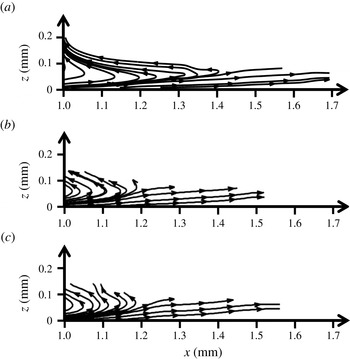
This appendix provides three different cross-sectional streamline maps. The streamlines are extracted from figure 9(a). As shown in figure 16, the streamlines are nearly parallel and straight along the
 $x$
direction. At
 $x=1.0\ \text{mm}$
, the liquid flow is extracted through the outlet and therefore there is a strong suction flow. In this study, we do not take into account this region.
Comparison of the streamlines at (a)
 $y=-0.04\ \text{mm}$
, (b)
 $y=-0.19\ \text{mm}$
, and (c)
 $y=0.23\ \text{mm}$
.

Appendix B. Comparison of analytical results between low Reynolds number and intermediate Reynolds number examples
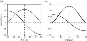
Snoeijer et al. (Reference Snoeijer, Rio, Le Grand and Limat2005) first showed the self-similar flow pattern in the corner structure at
 $\mathit{Re}\ll 1$
. Interestingly, this similarity occurs over a wide range of Reynolds numbers, i.e. for both a droplet sliding down an incline (
 $\mathit{Re}\ll 1$
) and a liquid immersion droplet (
 $\mathit{Re}\sim O(100)$
). If the dynamic pressure is neglected in (4.13), then the velocity expressions are same as the result of Snoeijer et al. (Reference Snoeijer, Rio, Le Grand and Limat2005). For
 ${\rm\Phi}=40^{\circ }$
and 75°, we compare the analytical velocity profiles for both problems, as shown in figure 17 where the velocity components are normalized by the relative droplet velocity,
 $U$
. Surprisingly, the two solutions are more or less identical, although the differential equations are not identical, cf. (4.9) and equation (8) by Limat & Stone (Reference Limat and Stone2004) and equation (10) by Snoeijer et al. (Reference Snoeijer, Rio, Le Grand and Limat2005). In the case of
 ${\rm\Phi}=75^{\circ }$
, the two solutions are exactly same, and the
 $U_{r}$
and
 $U_{{\it\phi}}$
profiles collapse as shown in figure 17(a). In the case of
 ${\rm\Phi}=40^{\circ }$
, the velocity profiles are only slightly different (figure 17
b).
Comparison of analytical velocity profiles for (a)
 ${\rm\Phi}=75^{\circ }$
and (b)
 ${\rm\Phi}=40^{\circ }$
. The solid line is the analytical solution based on the Stokes flow by Snoeijer et al. (Reference Snoeijer, Rio, Le Grand and Limat2005) and the dashed line is for (4.13) based on the modified lubrication theory.

As shown in figure 17, both results show that the velocity profiles are independent of the local distance. In particular, the radial velocity component
 $U_{r}$
becomes zero close to the contact line, and the angular velocity can be approximated as
 $U_{{\it\phi}}\cong -U\ \sin {\rm\Phi}$
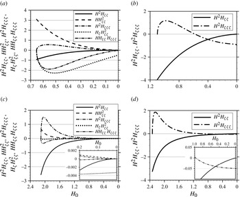
. To interpret the difference between the two analytical solutions, we plot the profile of each derivative term of (4.13) of this paper and equation (13) of Snoeijer et al. (Reference Snoeijer, Rio, Le Grand and Limat2005) in figure 18. If
 $H(0)$
approaches 0, it means that
 ${\it\phi}\rightarrow {\rm\Phi}$
. On the other hand, when
 $H(0)=H_{0}$
, i.e. the centreline of the partial dewetting flow,
 ${\it\phi}\rightarrow 0$
. For the problem in the Stokes flow regime,
 $H^{2}H_{{\it\zeta}{\it\zeta}}\rightarrow 0$
as
 $H\rightarrow 0$
. At the contact line, the
 $H^{2}H_{{\it\zeta}{\it\zeta}{\it\zeta}}$
term determines the angular velocity
 $U_{{\it\phi}}$
and then
 $U_{{\it\phi}}=UH^{2}H_{{\it\zeta}{\it\zeta}{\it\zeta}}/3\cos ^{3}{\rm\Phi}$
. On the other hand, in the case of the problem considering dynamic pressure effects, all the terms except for
 $H_{{\it\zeta}}H_{{\it\zeta}{\it\zeta}}^{2}$
vanish at the contact line. Therefore, for the angular velocity component
 $U_{{\it\phi}}$
at the contact line,
 $U_{{\it\phi}}=-UH_{{\it\zeta}}H_{{\it\zeta}{\it\zeta}}^{2}/3\cos ^{5}{\rm\Phi}$
. This result can also be obtained from (4.9). If
 ${\it\zeta}$
approaches the contact line,
 ${\it\zeta}\rightarrow \tan {\rm\Phi}$
, (4.9) is dominated by the highest order of
 ${\it\zeta}$
. Hence, (4.9) reduces to
 $$\begin{eqnarray}-3\left(\tan {\rm\Phi}\right)H_{{\it\zeta}}\cong -(1+\tan ^{2}{\rm\Phi})^{3}\left(-HH_{{\it\zeta}}H_{{\it\zeta}{\it\zeta}}^{2}+2H^{2}H_{{\it\zeta}{\it\zeta}}H_{{\it\zeta}{\it\zeta}{\it\zeta}}\right)_{{\it\zeta}},\end{eqnarray}$$
where
 ${\it\zeta}\rightarrow \tan {\rm\Phi}$
, and we integrate this with respect to
 ${\it\zeta}$
once, to give
 $$\begin{eqnarray}3\sin {\rm\Phi}\cos ^{5}{\rm\Phi}=-H_{{\it\zeta}}H_{{\it\zeta}{\it\zeta}}^{2}+2HH_{{\it\zeta}{\it\zeta}}H_{{\it\zeta}{\it\zeta}{\it\zeta}}+\frac{C}{H},\end{eqnarray}$$
where
 $C$
is an integration constant which is zero to prevent the divergence of the equation when
 $H\rightarrow 0$
. Furthermore,
 $HH_{{\it\zeta}{\it\zeta}}H_{{\it\zeta}{\it\zeta}{\it\zeta}}\rightarrow 0$
and
 $H_{{\it\zeta}}H_{{\it\zeta}{\it\zeta}}^{2}$
has a finite value, when
 $H\rightarrow 0$
. Therefore, we have
 $\sin {\rm\Phi}=-H_{{\it\zeta}}H_{{\it\zeta}{\it\zeta}}^{2}/(3\cos ^{5}{\rm\Phi})$
at the contact line. From the analytical velocity profile, we show that the angular velocity at the contact line (
 $H\rightarrow 0$
) is
 $U_{{\it\phi}}=-UH_{{\it\zeta}}H_{{\it\zeta}{\it\zeta}}^{2}/3\cos ^{5}{\rm\Phi}$
. Thus, we obtain the same result
 $U_{{\it\phi}}\cong -U\sin {\rm\Phi}$
, as shown in figure 17. Although the value to determine the velocity profile is different, the result shows a self-similar flow pattern when the rear shape of the droplet has a corner. Moreover, the interesting result is that the flow pattern is determined by the interface equation
 $H({\it\zeta})$
, i.e. the shape of the droplet tail.
Derivative term profiles in the velocity profiles: (a,b) are for
 ${\rm\Phi}=40^{\circ }$
and (c,d) are for
 ${\rm\Phi}=75^{\circ }$
; (a,c) are for the theory including inertia, while (b,d) are for the Stokes case.