1 Introduction
It has long been established that in partially or fully unconfined turbulent flows, such as jets, wakes and boundary layers, regions of turbulent and non-turbulent flow are separated by sharp and strongly contorted interfaces (e.g. Corrsin & Kistler Reference Corrsin and Kistler1954; Da Silva et al.
Reference Da Silva, Hunt, Eames and Westerweel2014). Interest in these turbulent/non-turbulent interfaces (TNTIs) has remained high since they play a crucial role in setting the entrainment rate, which is an important parameter in many practical applications. In particular, when following the conventional approach of defining the instantaneous TNTI using an appropriate threshold on enstrophy
 $\unicode[STIX]{x1D714}^{2}$
, where
 $\unicode[STIX]{x1D714}$
denotes the norm of the vorticity vector, a local entrainment velocity describing the motion of the TNTI relative to the fluid can be computed from
 $v_{n}\equiv -|\unicode[STIX]{x1D735}\unicode[STIX]{x1D714}^{2}|^{-1}\,\text{D}\unicode[STIX]{x1D714}^{2}/\text{D}t$
(Holzner & Lüthi Reference Holzner and Lüthi2011). The entrained volume flux is then given by the surface integral
 $$\begin{eqnarray}Q_{\unicode[STIX]{x1D714}}\equiv \int _{A_{\unicode[STIX]{x1D702}}}v_{n}\,\text{d}A=\langle v_{n}\rangle A_{\unicode[STIX]{x1D702}},\end{eqnarray}$$
where
 $\langle \cdot \rangle$
denotes an average over the surface area of the TNTI,
 $A_{\unicode[STIX]{x1D702}}$
. While
 $v_{n}$
is widely observed to be of the order of the small-scale (Kolmogorov) velocity
 $u_{\unicode[STIX]{x1D702}}$
(Holzner & Lüthi Reference Holzner and Lüthi2011), the multiscale aspect of turbulent entrainment is reflected in
 $A_{\unicode[STIX]{x1D702}}$
, which is set by eddies distorting the TNTI across the full range of scales.
The flow case under consideration here is a gravity current originating from a continuous release of heavier fluid along a sloping bottom into uniform surroundings. This problem was originally investigated by Ellison & Turner (Reference Ellison and Turner1959), who found that the entrainment parameter
 $E$
is a decreasing function of the Richardson number,
 $Ri$
, which represents the ratio of the competing forces of stratification and shear (see § 3 for exact definitions). A sound understanding of how
 $E$
varies depending on the flow parameters is important, e.g., in the study of turbidity currents, where surprisingly high runout lengths have been linked to very low entrainment rates (Sequeiros et al.
Reference Sequeiros, Spinewine, Beaubouef, Sun, García and Parker2010; Sequeiros Reference Sequeiros2012; Kneller et al.
Reference Kneller, Nasr-Azadani, Radhakrishnan and Meiburg2016). In a recent effort to elucidate this behaviour of
 $E$
in relation to properties of the TNTI, Krug et al. (Reference Krug, Holzner, Lüthi, Wolf, Kinzelbach and Tsinober2015) showed that the reduction of
 $E$
is in significant part due to a decrease of
 $A_{\unicode[STIX]{x1D702}}$
with increasing
 $Ri$
, whereas
 $\langle v_{n}\rangle /u_{\unicode[STIX]{x1D702}}$
remains largely unaffected. Their experimental findings have since been confirmed by the direct numerical simulations (DNS) of van Reeuwijk, Krug & Holzner (Reference van Reeuwijk, Krug and Holzner2017). A key to understanding the entrainment rate in gravity currents – and quite possibly also to modelling it – therefore lies in understanding the behaviour of
 $A_{\unicode[STIX]{x1D702}}$
. Hence, the goal of the present study is to investigate stratification effects on
 $A_{\unicode[STIX]{x1D702}}$
using a multiscale approach. The analytical tools necessary are available from numerous related studies on flows without a stable density stratification, which are summarized in the review of Sreenivasan (Reference Sreenivasan1991). Their most relevant result is the prediction of fractal scaling in the inertial region based on the proposal of scale invariance for turbulent geometries by Mandelbrot (Reference Mandelbrot1982). Fractal scaling for the TNTI implies power-law behaviour according to Sreenivasan, Ramshankar & Meneveau (Reference Sreenivasan, Ramshankar and Meneveau1989),
 $$\begin{eqnarray}A_{\unicode[STIX]{x1D702}}=A_{0}(l_{i}/l_{o})^{2-D_{f}},\end{eqnarray}$$
where
 $l_{i}$
and
 $l_{o}$
are the inner and outer cutoffs of the inertial scaling range respectively. Theoretical predictions yield
 $D_{f}=7/3$
for the fractal dimension, in good agreement with recent high-Reynolds-number (
 $Re$
) experiments by de Silva et al. (Reference de Silva, Philip, Chauhan, Meneveau and Marusic2013), who find
 $D_{f}\approx 2.3{-}2.4$
for the TNTI in turbulent boundary layers. It should be noted that others (e.g. Dimotakis & Catrakis Reference Dimotakis, Catrakis, Chaté, Villermaux and Chomaz1999) argue that
 $D_{f}$
should be scale-dependent. However, a significant scale separation is required to address this issue, and this will not be the focus here. The goal of the present study is to ascertain how the previously observed decrease of
 $A_{\unicode[STIX]{x1D702}}/A_{0}$
with increasing
 $Ri$
is reflected in changes of the fractal scaling parameters
 $l_{i}$
,
 $l_{o}$
and
 $D_{f}$
compared with the unstratified case where
 $Ri=0$
. To this end, we make use of DNS of a temporal version of the gravity current problem previously introduced in van Reeuwijk et al. (Reference van Reeuwijk, Krug and Holzner2017). Before presenting our results in § 3 followed by a discussion in § 4, details of the simulations are given in § 2. Our conclusions are summarized in § 5.
2 Simulations
In the temporal gravity current simulated here, the flow evolves in time (instead of along the streamwise coordinate as in the spatial case) due to periodic boundary conditions not only in the spanwise but also in the streamwise direction. A detailed discussion of the concept and the numerical configuration used was recently provided in van Reeuwijk et al. (Reference van Reeuwijk, Krug and Holzner2017), who also confirmed that the aforementioned findings of Krug et al. (Reference Krug, Holzner, Lüthi, Wolf, Kinzelbach and Tsinober2015) transfer to the temporal problem. The simulations presented here were carried out using a fourth-order accurate discretization of the Navier–Stokes equations in the Boussinesq approximation (Craske & van Reeuwijk Reference Craske and van Reeuwijk2015). The flow is initialized with uniform distributions of streamwise velocity
 $u_{0}$
and buoyancy
 $b_{0}$
up to a height
 $h_{0}$
above the bottom wall (located at
 $z=0$
), and is statistically homogeneous in the streamwise (
 $x$
) and spanwise (
 $y$
) directions. The buoyancy vector is given by
 $\boldsymbol{b}=b\hat{\boldsymbol{g}}$
, where
 $b$
is a scalar with Schmidt number
 $Sc=1$
and the unit vector
 $\hat{\boldsymbol{g}}$
is tilted at an angle
 $\unicode[STIX]{x1D6FC}$
with respect to the vertical (i.e. the
 $z$
axis) in order to simulate a sloping bottom. Hence, the component
 $b\sin (\unicode[STIX]{x1D6FC})$
drives the flow along
 $x$
, while
 $b\cos (\unicode[STIX]{x1D6FC})$
is causing a stable stratification in the wall-normal direction. Throughout this paper, we make use of the top-hat definitions
 $$\begin{eqnarray}u_{T}h=\int _{0}^{\infty }\overline{u}\,\text{d}z,\quad u_{T}^{2}h=\int _{0}^{\infty }\overline{u}^{2}\,\text{d}z\quad \text{and}\quad b_{T}h=\int _{0}^{\infty }\overline{b}\,\text{d}z=B_{0},\end{eqnarray}$$
where
 $u$
is the streamwise velocity (the overline indicates averaging in wall-parallel planes; the corresponding fluctuations are given by
 $u^{\prime }=u-\overline{u}$
) and the buoyancy content
 $B_{0}$
is a conserved quantity in the temporal problem (van Reeuwijk et al.
Reference van Reeuwijk, Krug and Holzner2017). The velocity components along the
 $y$
- and
 $z$
-axes are denoted by
 $v$
and
 $w$
respectively. With the above definitions, we can form a bulk Reynolds number
 $Re=u_{T}h/\unicode[STIX]{x1D708}$
, where
 $\unicode[STIX]{x1D708}$
is the kinematic viscosity, and a Richardson number
 $Ri=B_{0}\cos (\unicode[STIX]{x1D6FC})/u_{T}^{2}$
. Table 1 summarizes the parameters of the simulations employed in this study. For the gravity currents (labelled GCs in the following),
 $Ri_{0}$
is varied by changing the inclination angle
 $\unicode[STIX]{x1D6FC}$
while keeping the integral forcing
 $\sin (\unicode[STIX]{x1D6FC})B_{0}$
in the
 $x$
-direction constant. In addition, we ran a simulation with the buoyancy term switched off, resulting in an unstratified (temporal) wall jet (WJ) that is driven by initial momentum only. Apart from the bulk flow behaviour, where the whole domain was used, results will be based on averages over six independent
 $xz$
-planes, which are spaced equally in the
 $y$
-direction, amounting to 250 snapshots over a period of 120
 $h_{0}/u_{0}$
.
Simulation parameters:
 $N_{i}$
and
 $L_{i}$
denote the number of grid points and the domain size along the
 $i$
-direction respectively; subscript ‘0’ marks quantities at the start of the simulation. Results for
 $\hat{Re}_{\unicode[STIX]{x1D706}}$
are averaged over
 $100<\tilde{t}<120$
.

3 Results
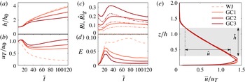
The bulk flow behaviour in terms of
 $h$
and
 $u_{T}$
is presented in figure 1 as a function of the dimensionless time
 $\tilde{t}=tu_{0}/h_{0}$
. After an initial transient, these quantities are observed to evolve conforming to their inviscid scaling
 $h\propto \tilde{t}$
and
 $u_{T}\propto \text{const.}$
for GCs, and
 $h\propto \tilde{t}^{1/2}$
and
 $u_{T}\propto \tilde{t}^{-1/2}$
for the WJ (van Reeuwijk et al.
Reference van Reeuwijk, Krug and Holzner2017), with a clear trend of decreasing
 $h$
and increasing
 $u_{T}$
with increasing
 $Ri_{0}$
. As figure 1(c) shows,
 $Ri$
asymptotes towards different constants for
 $\tilde{t}\gtrsim 90$
for the GC simulations. In accordance with previous findings, this relates also to different values of the entrainment parameter
 $E$
shown in figure 1(d), which is defined as
 $E=u_{T}^{-1}\,\text{d}h/\text{d}t$
for temporal flows. In equilibrium flow, both
 $Ri\rightarrow \text{const.}$
and
 $E\rightarrow \text{const.}$
, such that figure 1(c,d) provides further indicators that equilibrium has indeed been reached in the simulations. We further note that
 $E$
for all GCs is significantly reduced compared with the WJ, for which
 $Ri=0$
at all times.
Temporal evolution of (a) top-hat thickness
 $h$
, (b) top-hat velocity
 $u_{T}$
, (c)
 $Ri$
(thick) and
 $Ri_{g}$
(dashed-dotted lines) and (d) entrainment coefficient
 $E$
. (e) Mean profiles of streamwise velocity at
 $\tilde{t}=100$
, with the grey shading indicating the averaging band for turbulence quantities. The legend in (e) applies to all panels; the colour scheme is chosen such that darker shades of red correspond to larger
 $Ri$
.

The basic structure of the flow can be inferred from the profiles of
 $\overline{u}$
displayed in figure 1(e). Starting from the wall where
 $\overline{u}=0$
, the velocity increases sharply within the boundary layer up to a maximum at
 $z/h\approx 0.15$
, followed by a decrease back to zero at
 $z/h\approx 1.5$
. In the region
 $0.3<z/h<1.2$
, this decrease – and similarly the one for
 $\overline{b}$
(not shown) – is linear to a very good approximation. In order to exclude the influence of the near-wall region, where wall scaling prevails, from entering the statistics, we will restrict averages to this region in the following and denote this by using
 $\hat{(\cdot )}$
. As indicated in the figure,
 ${\hat{h}}=0.9h$
and
 $\hat{u} \approx 1.1u_{T}$
, and we define the gradient Richardson number as
 $\hat{Ri}_{g}=(\hat{N}/{\hat{S}})^{2}$
, where
 $\hat{N}^{2}=\text{d}\overline{b}/\text{d}z$
is the buoyancy frequency and
 ${\hat{S}}=\text{d}\overline{u}/\text{d}z$
is the shear. Results for
 $\hat{Ri}_{g}$
are also included in figure 1(c) (dashed-dotted lines), and it is obvious that the behaviour resembles that of
 $Ri$
with slightly lower magnitudes. Furthermore, we point out that even though there are fundamental differences between the WJ and the GCs, the collapse in figure 1(e) indicates that the structures of the flows are indeed very similar.
The position of the TNTI is detected using a threshold on the enstrophy
 $\unicode[STIX]{x1D714}^{2}=\unicode[STIX]{x1D714}_{i}\unicode[STIX]{x1D714}_{i}$
, where
 $\unicode[STIX]{x1D714}_{i}$
is the vorticity vector. For simplicity, a single threshold value
 $\unicode[STIX]{x1D714}_{thr}^{2}=3\times 10^{-5}u_{0}^{2}/h_{0}^{2}$
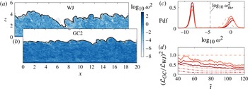
is chosen here at all times and for all flows. Two sample
 $\unicode[STIX]{x1D714}^{2}$
-snapshots in figure 2(a,b) for WJ and GC2 provide evidence for the suitability of this criterion. These figures further demonstrate that the location of the TNTI hardly changes even when varying the threshold value over a range of four orders of magnitude in total. Consequently, the results presented in the following are also largely independent of the exact choice of
 $\unicode[STIX]{x1D714}_{thr}^{2}$
. Further, figure 2(c) presents a probability density function of
 $\log _{10}\unicode[STIX]{x1D714}^{2}$
at the end of the simulations, when the differences between the flows are maximal. The distribution is bimodal, with the peaks corresponding to the turbulent region (high
 $\unicode[STIX]{x1D714}^{2}$
) and an essentially irrotational region (low
 $\unicode[STIX]{x1D714}^{2}$
). From this figure, it is clear that the threshold is suitably chosen to differentiate between the two regions.
Snapshots of the enstrophy distribution in (a) WJ at
 $\tilde{t}=60$
and (b) GC2 at
 $\tilde{t}=90$
, with the times selected such that
 $h=2.75$
in both flows. Black solid lines indicate the position of the TNTI along with isocontours at
 $100\unicode[STIX]{x1D714}_{thr}^{2}$
(dash-dotted) and
 $0.01\unicode[STIX]{x1D714}_{thr}^{2}$
(dotted). (c) Probability density function (p.d.f.) of
 $\log _{10}\unicode[STIX]{x1D714}^{2}$
at
 $\tilde{t}=120$
and (d) squared ratio of interface lengths
 $({\mathcal{L}}_{GC}/{\mathcal{L}}_{WJ})^{2}$
(thick lines) along with
 $E_{GC}/E_{WJ}$
(dash-dotted lines). The legend from figure 1(e) applies.

As a next step, we focus on the multiscale properties of the interface. For the ease of data handling and computation, instead of considering
 $A_{\unicode[STIX]{x1D702}}$
itself, we will consider its 2D surrogate in the following, which corresponds to the length
 ${\mathcal{L}}$
of the TNTI contours in snapshots such as those shown in figure 2(a,b). These snapshots were chosen such that
 $h$
is nominally the same, and it is obvious that in this case
 ${\mathcal{L}}_{WJ}$
is significantly larger than
 ${\mathcal{L}}_{GC2}$
. In order to relate results from
 $xz$
-snapshots to
 $A_{\unicode[STIX]{x1D702}}$
, it has to be assumed that interface convolutions in the
 $yz$
-plane are similar, which has been shown to be valid for wall jets (Paizis & Schwarz Reference Paizis and Schwarz1974). Accordingly, we plot
 $({\mathcal{L}}_{GC}/{\mathcal{L}}_{WJ})^{2}$
as a surrogate for
 $A_{\unicode[STIX]{x1D702},GC}/A_{\unicode[STIX]{x1D702},WJ}$
in figure 2(d). We note that this ratio reaches values as low as 0.5, which is of the order of the relative reduction in
 $E$
also plotted in the figure. This observation again emphasizes the important role the reduction of
 $A_{\unicode[STIX]{x1D702}}$
plays in reducing
 $E$
.
Since the quantity of interest here is the length
 ${\mathcal{L}}$
at different scales, we investigate the fractal scaling of the TNTI based on filtered fields similarly to de Silva et al. (Reference de Silva, Philip, Chauhan, Meneveau and Marusic2013). Before filtering, we transform
 $\unicode[STIX]{x1D714}^{2}$
to the binary field
 $I$
, where
 $I=1$
if
 $\unicode[STIX]{x1D714}^{2}\geqslant \unicode[STIX]{x1D714}_{thr}^{2}$
and
 $I=0$
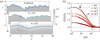
otherwise. As illustrated in figure 3, this field is then filtered according to
 $\tilde{I} =\int I(\boldsymbol{x}-\boldsymbol{x}^{\prime })G(\boldsymbol{x}^{\prime })\,\text{d}^{2}\boldsymbol{x}^{\prime }$
, with
 $G$
denoting the kernel of a square box-filter with filter width
 $\unicode[STIX]{x1D706}$
. In the filtered fields, the TNTI is then found where
 $\tilde{I} =0.5$
. The main advantage of this procedure as opposed to filtering
 $\unicode[STIX]{x1D714}^{2}$
directly is that it approximately preserves the mean interface position. Based on a self-similarity argument (van Reeuwijk & Holzner Reference van Reeuwijk and Holzner2014), this is a prerequisite to expecting fluxes across the TNTI evaluated at different scales to be equal, i.e.
 $Q_{\unicode[STIX]{x1D714}}(\unicode[STIX]{x1D706})=Q_{\unicode[STIX]{x1D714}}$
.
(a) Illustration of the filtering procedure applied to the
 $\unicode[STIX]{x1D714}^{2}$
-snapshot shown in figure 2(a). The blue line represents the TNTI at the respective filter scale. (b) Interface length
 ${\mathcal{L}}(\unicode[STIX]{x1D706})$
at
 $\tilde{t}=60$
for all simulations. The black solid line corresponds to the fit for WJ according to (3.1).

The equivalent of (1.2) for
 ${\mathcal{L}}$
evaluated at a filter scale is given by
 ${\mathcal{L}}(\unicode[STIX]{x1D706})\propto \unicode[STIX]{x1D706}^{-\unicode[STIX]{x1D6FD}}$
, where
 $\unicode[STIX]{x1D6FD}\approx 0.3$
–
 $0.4$
(de Silva et al.
Reference de Silva, Philip, Chauhan, Meneveau and Marusic2013). Sample results for
 ${\mathcal{L}}(\unicode[STIX]{x1D706})$
are depicted in figure 3(b), where
 $\unicode[STIX]{x1D706}$
is normalized by the Kolmogorov scale
 $\hat{\unicode[STIX]{x1D702}}=(\unicode[STIX]{x1D708}^{3}/\hat{\unicode[STIX]{x1D700}})^{1/4}$
and
 $\hat{\unicode[STIX]{x1D700}}$
is the rate of turbulent dissipation. The curves level off at small and large
 $\unicode[STIX]{x1D706}$
, which relate to the outer and inner cutoffs respectively. However, the transitions are smooth, such that the determination of
 $l_{i}$
and
 $l_{o}$
is not straightforward. Given the limited range of scales in the simulation, the slope
 $\unicode[STIX]{x1D6FD}$
will also vary depending on the chosen scaling range. To determine the fractal scaling parameters nevertheless in a consistent and unambiguous manner, despite the moderate
 $Re$
, we make use of the fit function
 $$\begin{eqnarray}\frac{{\mathcal{L}}(\unicode[STIX]{x1D706})}{L_{x}}=\left(\frac{l_{o}}{l_{i}}\right)^{\unicode[STIX]{x1D6FD}}\left[\frac{1+(\unicode[STIX]{x1D706}/l_{o})^{2}}{1+(\unicode[STIX]{x1D706}/l_{i})^{2}}\right]^{\unicode[STIX]{x1D6FD}/2}\end{eqnarray}$$
developed and tested by Thiesset et al. (Reference Thiesset, Maurice, Halter, Mazellier, Chauveau and Gökalp2016) for exactly this purpose. The function smoothly connects the asymptotes
 ${\mathcal{L}}=\text{const.}$
for
 $\unicode[STIX]{x1D706}\ll l_{i}$
and
 $\unicode[STIX]{x1D706}\gg l_{o}$
(where
 ${\mathcal{L}}/L_{x}=1$
) with the fractal scaling
 ${\mathcal{L}}/L_{x}\propto (l_{o}/\unicode[STIX]{x1D706})^{\unicode[STIX]{x1D6FD}}$
for
 $l_{i}\lesssim \unicode[STIX]{x1D706}\lesssim l_{o}$
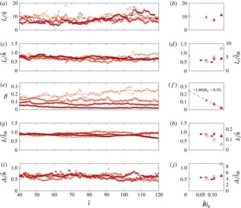
in a way that closely agrees with the data, as can be inferred from the representative fit in figure 3. Results from applying (3.1) to the data are presented in figure 4(a–f). While, predominantly due to limited statistics, there is some scatter in figure 4(a,c,e) between individual time steps, the time-averaged trends are robust and allow for firm conclusions. Judging from the fact that
 $l_{i}/\hat{\unicode[STIX]{x1D702}}$
is approximately constant in time (cf. figure 4
a) and indifferent to
 $\hat{Ri}_{g}$
(cf. figure 4
b), it is concluded that
 $l_{i}\propto \hat{\unicode[STIX]{x1D702}}$
, with
 $l_{i}\approx 10\hat{\unicode[STIX]{x1D702}}$
. Similarly, figure 4(c,d) suggests that
 $l_{o}\propto {\hat{h}}$
and
 $l_{o}\approx 0.6{-}0.8{\hat{h}}$
for the GCs as well as the WJ. For the scaling exponent
 $\unicode[STIX]{x1D6FD}$
in figure 4(e,f), however, significant differences appear. It is apparent – especially from the averages at late times in figure 4(f) – that
 $\unicode[STIX]{x1D6FD}$
is a decreasing function of
 $\hat{Ri}_{g}$
. For the WJ,
 $\unicode[STIX]{x1D6FD}$
takes significantly longer than for the GCs to approach a constant value and, presumably due to confinement effects, never reaches the theoretically predicted value of
 $1/3$
. The WJ grows fastest with the strongest interface contortions (see figures 1
a and 2
a) and is therefore most susceptible to interference due to the finite size of the computational domain. Based on the above results,
 ${\mathcal{L}}/L_{x}\propto (l_{o}/l_{i})^{\unicode[STIX]{x1D6FD}}\propto ({\hat{h}}/\hat{\unicode[STIX]{x1D702}})^{\unicode[STIX]{x1D6FD}}\propto (Re^{3/4})^{\unicode[STIX]{x1D6FD}}$
, and we note that
 $\unicode[STIX]{x1D6FD}$
is the decisive parameter in reducing
 ${\mathcal{L}}$
(or equivalently
 $A_{\unicode[STIX]{x1D702}}$
). In fact,
 $Re$
is larger for the GCs than for the WJ as the constant forcing
 $\sin \unicode[STIX]{x1D6FC}B_{0}$
keeps increasing the volume flux
 $u_{T}h$
. This also implies that the
 $\hat{Ri}_{g}$
trend of
 $\unicode[STIX]{x1D6FD}$
cannot be an artefact of an increasingly restricted scaling range as it is in fact becoming slightly larger. Even though the linear fit in figure 4(f) appears suggestive, it lacks a physical underpinning. With the caveat that
 $\unicode[STIX]{x1D6FD}(\hat{Ri}_{g}=0)$
is lower than the commonly accepted value of
 $\unicode[STIX]{x1D6FD}\approx 1/3$
in this case, it may however serve as an approximation at larger
 $\hat{Ri}_{g}$
.
Results from applying the fit (3.1): inner cutoff
 $l_{i}/\hat{\unicode[STIX]{x1D702}}$
(a,b), outer cutoff
 $l_{o}/{\hat{h}}$
(c,d) and slope
 $\unicode[STIX]{x1D6FD}$
(e,f), along with
 $\unicode[STIX]{x1D6FF}/\hat{l}_{Sk}$
(g,h) and
 $\unicode[STIX]{x1D6E5}/{\hat{h}}$
(i,j), plotted as function of
 $\tilde{t}$
(a,c,e,g,i), with black lines indicating a moving average over
 ${\approx}10\tilde{t}$
, and of
 $\hat{Ri}_{g}$
averaged over
 $100\leqslant \tilde{t}\leqslant 120$
(b,d,f,h,j). The legend from figure 3(b) applies; the open symbols in (d,h,j) relate to alternative normalizations on the right-hand axis. The dashed line in (f) represents a linear fit to the data with the parameters given in the figure.

The observation that
 $l_{o}\propto {\hat{h}}$
might appear surprising, as one would expect the large-scale cutoff in stratified (or sheared) flows to be determined by a buoyancy (shear) scale. In fact, with
 $\hat{Ri}_{g}<0.25$
(cf. figure 1
c), all flows considered here are ‘shear-dominated’ according to the framework of Mater & Venayagamoorthy (Reference Mater and Venayagamoorthy2014). In this regime, the largest scales are of the order of the shear scale
 $\hat{l}_{Sk}=(\hat{k}^{1/2}/{\hat{S}})$
, where
 $k$
is the turbulent kinetic energy. However, from the open symbols in figure 4(d), it becomes obvious that
 $\hat{l}_{Sk}$
is not the proper normalization for
 $l_{o}$
. In addition to the fit results already discussed, the length scale
 $\unicode[STIX]{x1D6FF}$
, which characterizes the wall-normal fluctuations of the interface position
 $z_{i}$
, is plotted in figure 4(g,h). It is defined by
 $\unicode[STIX]{x1D6FF}=\left[(1/{\mathcal{L}})\int (z_{i}(s)-\langle z_{i}\rangle )^{2}\,\text{d}s\right]^{1/2}$
, with
 $s$
denoting a curvilinear coordinate that runs along the TNTI. From the results in figure 4(g,h), there can be little doubt that
 $\unicode[STIX]{x1D6FF}(Ri_{g})$
scales on
 $\hat{l}_{Sk}$
and not
 ${\hat{h}}$
. In contrast, the scale
 $\unicode[STIX]{x1D6E5}$
, which is designed to characterize the streamwise extent of interface convolutions by measuring the mean streamwise distance of the zero crossings of the function
 $z_{i}-\langle z_{i}\rangle$
, is seen to scale on
 ${\hat{h}}$
(see figure 4
i,j). Hence, there is an anisotropy in the scaling relations, the implications of which we will discuss in the following.
4 Discussion
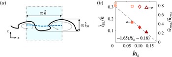
The situation at the interface is sketched in figure 5(a). The different scalings of
 $\unicode[STIX]{x1D6FF}$
and
 $\unicode[STIX]{x1D6E5}$
observed above suggest that eddies are distorted such that they produce convolutions whose size in
 $x$
is approximately
 ${\hat{h}}$
but that are limited to
 $\hat{l}_{Sk}$
in
 $z$
. The latter is consistent with the aforementioned shear cutoff and corresponds to the scaling expected in a homogeneous shear flow (Pope Reference Pope2000). However, the finite extent of the shear layer, which is
 $\propto {\hat{h}}$
, is seen to become relevant in the streamwise direction. This is consistent with the fact that the wavelength of the Kelvin–Helmholtz instability active here scales with the thickness of the shear layer (Schmid & Henningson Reference Schmid and Henningson2000).
(a) Schematic of the anisotropic interface geometry. The shaded blue area represents a filter and the dashed blue line the filtered interface. (b) The ratio
 $\hat{l}_{Sk}/{\hat{h}}$
as a function of
 $\hat{Ri}_{g}$
(filled symbols) along with a linear fit to the data (dashed line and fit parameters). Also shown on the right-hand axis is the ratio of r.m.s. velocity fluctuations
 ${\hat{w}}_{rms}/\hat{u} _{rms}$
(open symbols).

It is noteworthy that no comparable scaling anisotropy was detected in related studies on turbulent jets (Mistry et al.
Reference Mistry, Philip, Dawson and Marusic2016) or boundary layers (e.g. Corrsin & Kistler Reference Corrsin and Kistler1954). In fact, this is not surprising since to a first approximation
 $l_{Sk}\propto l^{\ast }$
(where
 $l^{\ast }$
is a transverse length scale of the jet or the boundary layer thickness) in these flows with no additional dependence on
 $Ri$
.
With the above results, we have
 $\unicode[STIX]{x1D6FF}/\unicode[STIX]{x1D6E5}\propto \hat{l}_{Sk}/{\hat{h}}$
, which is smaller than 1 in all cases, as figure 5(b) shows. In this case, the filter width at which interface convolutions will be removed is set by their streamwise extent, as the sketch in figure 5(a) illustrates, which is consistent with
 $l_{o}\propto {\hat{h}}$
from figure 4(c,d). The results in figure 5(b) indicate that the anisotropy implied by the different scaling relations in different directions becomes more pronounced with increasing
 $\hat{Ri}_{g}$
. We further note that from the definition of
 $\hat{l}_{Sk}$
, it follows that
 $\hat{l}_{Sk}=\hat{k}^{1/2}/S=\hat{k}^{1/2}/(\hat{u} /{\hat{h}})={\hat{h}}\hat{k}^{1/2}/\hat{u}$
, such that the ratio plotted in figure 5(b) is equivalent to the turbulent intensity
 $\hat{k}^{1/2}/\hat{u}$
. Also included in figure 5(b) is the ratio of root mean square (r.m.s.) velocity fluctuations in the wall-normal and streamwise directions. This ratio decreases much slower with
 $\hat{Ri}_{g}$
than
 $\hat{l}_{Sk}/{\hat{h}}$
or the turbulence intensity. Therefore, it follows that the decrease in
 $\hat{l}_{Sk}/{\hat{h}}$
is not predominantly related to increased anisotropy caused by the suppression of wall-normal velocity fluctuation due to the stable stratification. It is rather that – even as shear increases with increasing
 $\hat{Ri}_{g}$
(cf. the discussion of figure 1) – the flow becomes less efficient in producing turbulent fluctuations, resulting in lower turbulence intensities and thus lower
 $\hat{l}_{Sk}/{\hat{h}}$
.
(a) Illustration of the construction of the model fractal. (b) Sample fractals after five iterations; darker shades of blue indicate increasing iterations for
 $r=0.3$
. (c) Normalized length
 $\unicode[STIX]{x1D6EC}/\unicode[STIX]{x1D6EC}_{0}$
for the two fractals (symbols) and predictions from (4.3) (lines).

In the following, we will assess the effect of this disparity in length scales on the fractal slope
 $\unicode[STIX]{x1D6FD}$
by replicating the geometry of the TNTI by a simple model fractal. The construction principle for the fractal curve is depicted in figure 6(a). At iteration
 $n$
(represented by the grey line), the curve consists of
 $N$
line segments with length
 $l_{n}$
, such that its total length is
 $\unicode[STIX]{x1D6EC}_{n}=\unicode[STIX]{x1D6EC}(l_{n})=Nl_{n}$
. At the next iteration (blue line), a new point is introduced at a distance
 $rl_{n}$
from the centre of
 $l_{n}$
, where
 $r$
is an anisotropy parameter, and it follows that
 $$\begin{eqnarray}l_{n+1}=\left[\left(\frac{l_{n}}{2}\right)^{2}+(rl_{n})^{2}\right]^{1/2}=\frac{l_{n}}{2}m,\end{eqnarray}$$
with the abbreviation
 $m=(1+4r^{2})^{1/2}$
. Alternating the side at which the new point is placed for consecutive line segments, as is done for the two sample fractals in figure 6(b), ensures that the mean position of the curve is preserved. With (4.1), we find that
 $\unicode[STIX]{x1D6EC}_{n+1}=2Nl_{n+1}=Nl_{n}m$
, and the fractal scaling from
 $$\begin{eqnarray}\frac{\unicode[STIX]{x1D6EC}(l_{n+1})}{\unicode[STIX]{x1D6EC}(l_{n})}=m=\left(\frac{l_{n}}{l_{n+1}}\right)^{\unicode[STIX]{x1D6FD}_{m}}=\left(\frac{2}{m}\right)^{\unicode[STIX]{x1D6FD}_{m}},\end{eqnarray}$$
with
 $\unicode[STIX]{x1D6FD}_{m}=f(m)$
denoting the fractal exponent of the model. Solving (4.2) for
 $\unicode[STIX]{x1D6FD}_{m}$
yields
 $$\begin{eqnarray}\unicode[STIX]{x1D6FD}_{m}=\frac{\ln m}{\ln {\displaystyle \frac{2}{m}}},\end{eqnarray}$$
which is also confirmed by the plot of
 $\unicode[STIX]{x1D6EC}/\unicode[STIX]{x1D6EC}_{0}$
versus
 $l_{n}/l_{0}$
in figure 6(c). From figure 6(b,c), it also becomes clear that lower values of
 $r$
, i.e. stronger anisotropy, lead to lower fractal slopes
 $\unicode[STIX]{x1D6FD}_{m}$
, similar to what has been observed in figure 4.
If the decrease of
 $\unicode[STIX]{x1D6FD}$
is in fact related to the increasing degree of anisotropy witnessed in figure 5(b), it should now be possible to find a proportionality constant
 $r=C\hat{l}_{Sk}/{\hat{h}}$
of order unity, such that
 $\unicode[STIX]{x1D6FD}(\hat{l}_{Sk}/{\hat{h}})\approx \unicode[STIX]{x1D6FD}_{m}(r)$
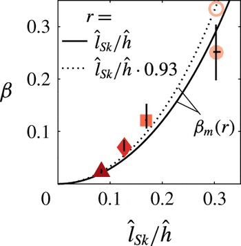
. Indeed, choosing
 $C=1$
yields reasonable agreement between
 $\unicode[STIX]{x1D6FD}$
and
 $\unicode[STIX]{x1D6FD}_{m}$
, as evidenced by the plot in figure 7. We recall that
 $\unicode[STIX]{x1D6FD}$
obtained from the present simulations for the WJ is lower than the established value of
 ${\approx}1/3$
, which is also included in figure 7. The correspondence between the data and the simple model is even better if this value is adopted along with
 $C=0.93$
.
The slope
 $\unicode[STIX]{x1D6FD}$
as a function of the ratio
 $\hat{l}_{Sk}/{\hat{h}}$
averaged over
 $100<\tilde{t}<120$
(filled symbols), with error bars indicating the full range of the data in that period. The open symbol marks the value of
 $\unicode[STIX]{x1D6FD}=1/3$
for the unstratified case. The lines represent
 $\unicode[STIX]{x1D6FD}_{m}$
according to (4.3) with
 $r=C\hat{l}_{Sk}/{\hat{h}}$
and different values of
 $C$
.

It should be noted that in deriving the model in its present form, it was assumed that
 $r$
, and hence the scaling anisotropy is independent of scale. Since results for both
 $\unicode[STIX]{x1D6FF}$
and
 $l_{o}$
are dominated by the largest scales, this is not strictly implied by the data. As outlined in the discussion of figure 5(b), the anisotropy of the TNTI is not directly related to anisotropy in the velocity field. It is rather a consequence of the fact that the streamwise and wall-normal directions have different characteristic length scales. Hence, the assumption of scale invariance of
 $r$
is not necessarily inconsistent with Kolmogorov’s hypothesis of small-scale isotropy. For a definitive answer as to whether
 $r=\text{const.}$
is in fact applicable even when the scaling range is large, data at significantly higher
 $Re$
would be required. In any case, a potential scaling transition can easily be accounted for in the model by rendering
 $r$
a function of the scale, essentially resulting in a multifractal object.
Moreover, if
 $\unicode[STIX]{x1D6FD}\rightarrow 0$
, then
 $A_{\unicode[STIX]{x1D702}}/A_{0}\rightarrow 1$
, and from (1.1)
 $v_{n}$
is no longer amplified by interface convolutions. The local entrainment velocity is dominated by viscous processes at small thresholds (e.g. Holzner & Lüthi Reference Holzner and Lüthi2011), and hence entrainment reduces to pure diffusion in this limit such that
 $E\rightarrow 0$
. Consistently, from extrapolating the direct measurements (figure 4
d), as well as the model (figures 5
b and 7), this limit is approached for
 $\hat{Ri}_{g}>0.15{-}0.18$
in our data, which (from figure 1
c) relates to
 $Ri\approx 0.2$
. We note that this value is significantly lower than the value of 0.8 predicted by the fit based on experimental data by Turner (Reference Turner1986). Presumably this is related to non-equilibrium effects in the experiment, but we reserve a detailed discussion for a future publication in order to limit the scope of the present paper.
5 Concluding remarks
Recent studies link the reduction of entrainment with increasing stratification in gravity currents to a decrease of the surface area
 $A_{\unicode[STIX]{x1D702}}$
of the TNTI. Here, we examined the multiscale properties of this effect using DNS of flows in a range from unstratified to strongly stratified conditions characterized by the Richardson number
 $\hat{Ri}_{g}$
. It was shown that the reduction of
 $A_{\unicode[STIX]{x1D702}}$
with increasing
 $\hat{Ri}_{g}$
is linked to a decrease in the fractal scaling exponent
 $\unicode[STIX]{x1D6FD}$
, while the inner and outer cutoffs of the scaling regime remain largely unaffected. Our results further show that interface convolutions scale differently in the streamwise and wall-normal directions. The former scales on the bulk scale
 ${\hat{h}}$
consistent with the underlying instability mechanism, while the latter scales on the shear scale
 $\hat{l}_{Sk}$
, which is the large-scale cutoff in shear-dominated flows such as the present ones. This went unnoticed in previous studies since the two different scalings coincide in neutrally buoyant flows. The ratio
 $\hat{l}_{Sk}/{\hat{h}}$
and hence the anisotropy of the bulges were seen to decrease with increasing
 $\hat{Ri}_{g}$
. It was finally found that a simple fractal model based on this finding convincingly predicts the dependence of
 $\unicode[STIX]{x1D6FD}$
on
 $\hat{Ri}_{g}$
. By allowing
 $A_{\unicode[STIX]{x1D702}}$
to be parametrized in terms of basic turbulence quantities, these novel results may play an important role in modelling turbulent entrainment. Moreover, it appears likely that the present findings might – at least in part – also transfer to other problems such as the deepening of the wind-mixed layer (Pollard, Rhines & Thompson Reference Pollard, Rhines and Thompson1972).