4.1. Dispersion and anisotropy

Firstly, the global features of the 2H$_2$–O$_2$–7Ar and 2H$_2$–O$_2$ mixtures are depicted using the instantaneous 2-D flow fields in figures 2 and 3, respectively. In the 2$\textrm {H}_2$–$\textrm {O}_2$–7Ar mixture, the cellular structure is regular with two cells in the channel (figure 2c). No unburned gas pocket is formed behind the front and the classical key stone feature can be observed (figure 2a,b). As for the 2$\textrm {H}_2$–$\textrm {O}_2$ mixture, the cellular structure and the frontal shape were more irregular (figure 3), expected from the increased instability parameters. The unburned gas pockets are torn apart from the front and continue to burn downstream (figure 3a,b). In both cases, strong transverse wave structures occurred in the second part of the cell (figures 2b and 3b), as also observed experimentally by Desbordes & Presles (Reference Desbordes and Presles2012). The thermicity fields indicated that the heat release took place much more rapidly and sometimes one order of magnitude quicker in the non-diluted case than in the diluted case (figures 2b and 3b). The average propagation velocity for both mixtures agreed with that of the CJ velocity. The average cell width in the simulations from the manual measurement of 150 and 300 cells for the 2$\textrm {H}_2$–$\textrm {O}_2$–7Ar and 2$\textrm {H}_2$–$\textrm {O}_2$ mixtures is 1.3 and 0.7 mm, respectively. The experimental cell width for the 2$\textrm {H}_2$–$\textrm {O}_2$–7Ar mixture is expected to be 2.7–4.0 mm from similar mixture conditions, and the cell width reported from experiments for the 2$\textrm {H}_2$–$\textrm {O}_2$ mixture ranges from 1.4 to 2.1 mm (Kaneshige & Shepherd Reference Kaneshige and Shepherd1997). Therefore, the cell sizes in the simulations were thus smaller that the experimental ones by a factor of approximately 2–3. The numerical cell width is reported to be smaller as in previous studies (Taylor et al. Reference Taylor, Kessler, Gamezo and Oran2013; Taileb et al. Reference Taileb, Meluguizo-Gavilances and Chinnayya2021a). This is not due to the present numerical resolution but may be due to vibrational non-equilibrium effects (Taylor et al. Reference Taylor, Kessler, Gamezo and Oran2013; Shi et al. Reference Shi, Shen, Zhang, Zhang and Wen2017), uncertainties of the chemical reaction model in detonation conditions (Mével & Gallier Reference Mével and Gallier2018) and three-dimensional (3-D) effects (Taileb et al. Reference Taileb, Reynaud, Chinnayya, Virot and Bauer2018; Monnier et al. Reference Monnier, Rodriguez, Vidal and Zitoun2022; Crane et al. Reference Crane, Lipkowicz, Shi, Wlokas, Kempf and Wang2023).

Figure 2.

The 2-D instantaneous flow fields in 2H$_2$–O$_2$–7Ar mixture: (a) temperature; (b) thermicity; (c) maximum pressure.

Figure 3.

The 2-D instantaneous flow fields in 2H$_2$–O$_2$ mixture: (a) temperature; (b) thermicity, (c) maximum pressure.

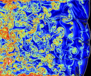
Figures 4 and 5 show the instantaneous 2-D flow fields in the Lagrangian perspective for (a) time front shock passage; (b) longitudinal distance travelled by the particle $x_{i}$; (c) transverse distance travelled by the particle $y_{i}$; (d) distance travelled by the particle $x_{{xy,i}}$ from shock passage for the 2H$_2$–O$_2$–7Ar and 2H$_2$–O$_2$ mixtures, respectively. As we move away from the leading shocks, the time from shock passage and the longitudinal distance $x_{i}$ increased. However, their distributions were not uniform in each section, regardless of the mixture instability. This non-uniform distribution of the Lagrangian particles is consistent with the numerical findings of Sow et al. (Reference Sow, Lau-Chapdelaine and Radulescu2021). The scales of the legends for figures 4(a) and 5(a) are different, due to the difference in detonation velocities for both mixtures. It can also be seen that $x_{i}$ and $x_{{xy},i}$ were almost the same, due to the fact that $y_{i}$ remained one order of magnitude lower. In the rest of the paper, only the field of $x_{i}$ will be discussed instead of that of $x_{{xy},i}$. More noticeable was that the transverse distance $y_{i}$ was much spottier for the non-diluted case, as we moved away from the leading shocks, indicative of more vortical structures. Large tongues of gas were also seen to penetrate the different layers and to be entrained in the $x$-direction. The longitudinal distance $x_{i}$ for the particles inside the boundary layer can also be seen to be shorter than that of the other particles in the core of the flow.

Figure 4.

The 2-D instantaneous Lagrangian flow fields in 2H$_2$–O$_2$–7Ar mixture, superimposed with Schlieren density: (a) time from shock passage; (b) longitudinal distance travelled by the Lagrangian particle $x_{i}$; (c) transverse distance travelled by the Lagrangian particle $y_{i}$; (d) distance travelled by the Lagrangian particle $x_{{xy},i}$.

Figure 5.

The 2-D instantaneous Lagrangian flow fields in 2H$_2$–O$_2$ mixture, superimposed with Schlieren density: (a) time from shock passage; (b) longitudinal distance travelled by the Lagrangian particle $x_{i}$; (c) transverse distance travelled by the Lagrangian particle $y_{i}$; (d) distance travelled by the Lagrangian particle $x_{{xy},i}$.

In order to compare the distribution of the distances for both mixtures, the average longitudinal distance $\bar {x}_{i}$ is shown in figure 6. The slopes are different due to the difference in the velocity induced by detonation of both mixtures. The standard deviation for $x_{i}$ (see figure 7a) $[ \sum _i^N (x_{i} - \bar {x}_{i})^2 /N ]^{1/2}$ were almost the same. The average transverse distance $\overline {y}_{i}$ (see figure 7b) can be as high as twice for the non-diluted as compared with the more stable case.

Figure 6.

Average longitudinal distance $\bar {x}_{i}$ for 2H$_2$–O$_2$–7Ar and 2H$_2$–O$_2$ mixtures.

Figure 7.

(a) Standard deviation for the longitudinal distance $[ \sum _i^N (x_{i} - \bar {x}_{i})^2 /N ]^{1/2}$ and (b) average transverse distance $\overline {y}_{i}$ for 2H$_2$–O$_2$–7Ar and 2H$_2$–O$_2$ mixtures.

Figures 8(a,b) and 9(a,b) depict the joint probability density function (p.d.f.) between the times from shock passage and the longitudinal and transverse distances travelled by the particles. The width of the distributions became wider as the time from the shock passage increased. The fluctuations along the transverse distance $y_{i}$ also increased (see figures 8d and 9d). From figures 8(c,d) and 9(c,d), the peak of the p.d.f. for the fluctuations along the longitudinal direction was lower than that of the transverse direction, meaning that the dispersion along the longitudinal direction was greater than that of the transverse one. This finding that the dispersion along the longitudinal direction was greater than that of the transverse wave was not what could be expected from the presence of the transverse waves, characteristics and cornerstones of the detonation cellular structure. Moreover, the comparison of figures 8(c,d) and 9(c,d) showed that the diluted case needed approximately five times more time to obtain the same level of dispersion than the non-diluted one. Indeed, the average transverse distance $\overline {y_{i}}$ became approximately one cell width after $17.8\,\mathrm {\mu }$s for the argon diluted case as compared with $3.6\,\mathrm {\mu }$s for the other case (figure 7b).

Figure 8.

The 2H$_2$–O$_2$–7Ar mixture. Joint p.d.f. between (a) times from shock passage and longitudinal distances $x_{i}$, (b) times from shock passage and transverse distances $y_{i}$. The p.d.f. at different instants for (c) longitudinal distances $x_{i}$ and distances $x_{{xy},i}$, (d) transverse distances $y_{i}$.

Figure 9.

The 2H$_2$–O$_2$ mixture. Joint p.d.f. between (a) times from shock passage and longitudinal distances $x_{i}$, (b) times from shock passage and transverse distances $y_{i}$. The p.d.f. at different instants for (c) longitudinal distances $x_{i}$ and distances $x_{{xy},i}$, (d) transverse distances $y_{i}$.

The 2-D instantaneous Lagrangian flow fields of the normalized fluctuations in the longitudinal distance ($\delta x_{i} = (x_{i}- \bar {x}_{i}) / x_{i}$) and the normalized transverse distance $y_{i}/x_{i}$ have been plotted in figures 10 and 11 for both cases. Near the front, they came mainly from three factors. At first, the triple point collision resulted in forward jets with positive $\delta x_{i}$ and in backward jets with negative values. Second, the decaying incident shock in the second part of the cell induced negative values. Finally, the transverse waves and the vortical motions played a major role in increasing $y_{i}$, the more important contribution coming from the latter, as time passed. Some differences were also present for $\delta x_{i}$ near the boundary layer. The fluctuations appeared spottier in the more unstable non-diluted case, with vortical motions also playing a stronger role in the unstable case.

Figure 10.

Diluted 2H$_2$–O$_2$–7Ar mixture. The 2-D instantaneous Lagrangian flow fields, superimposed with Schlieren density in diluted 2H$_2$–O$_2$–7Ar mixture. (a) Normalized fluctuations of the longitudinal distances $(x_{i}- \bar {x}_{i}) / x_{i}$. (b) Normalized transverse distance $y_{i}/x_{i}$.

Figure 11.

Non-diluted 2H$_2$–O$_2$ mixture. The 2-D instantaneous Lagrangian flow fields, superimposed with Schlieren density in diluted 2H$_2$–O$_2$–7Ar mixture. (a) Normalized fluctuations of the longitudinal distances $(x_{i}- \bar {x}_{i}) / x_{i}$. (b) Normalized transverse distance $y_{i}/x_{i}$.

Figure 12 shows the time history of the variances of the $x$- and $y$- displacements $\overline {x'^2_{{i}}}$ and $\overline {y'^2_{{i}}}$, as well as their correlation $\overline {x'_{{i}} y'_{{i}}}$, which can be evaluated by

(4.1)\begin{gather} \overline{x'^2_{{i}}} = \frac{1}{N} \sum_{i=1}^N \left[ (x_{{p},i} - x_{{p},i,0}) - \overline{(x_{{p},i} - x_{{p},i,0})} \right]^2 = \frac{1}{N} \sum_{i=1}^N \left( x_{i} - \overline{x_{i}} \right)^2, \end{gather}

(4.2)\begin{gather}\overline{y'^2_{{i}}} = \frac{1}{N} \sum_{i=1}^N ( y_{{p},i} - y_{{p},i,0} )^2, \end{gather}

(4.3)\begin{gather}\overline{x'_{{i}} y'_{{i}}} = \frac{1}{N} \sum_{i=1}^N \left[ (x_{{p},i} - x_{{p},i,0}) - \overline{(x_{{p},i} - x_{{p},i,0})} \right]\! ( y_{{p},i} - y_{{p},i,0} ). \end{gather}

Here, $x_{{p},i,0}$ and $y_{{p},i,0}$ are $x$ and $y$ initial positions of the particle $i$, and $N$ is the number of particles.

Figure 12.

(a) Time history of the variance of the $x$- and $y$- displacements, $\overline {x'^2_{i}}$ and $\overline {y'^2_{i}}$; (b) non-dimensionalized $y$- displacements, $\overline {y'^2_{i}} / \overline {x'^2_{i}}$ as a function of the non-dimensionalized time $\tau / \tau _{ind}$; (c) $\overline {x'_{i} y'_{i}} / (\overline {x'^2_{i}} + \overline {y'^2_{i}})$; (d) non-dimensionalized $x$- displacements, $\overline {x'^2_{i}} / (E_{a} /(RT_{vN}) x_{ind} )^2$ as a function of the non-dimensionalized time $\tau / \tau _{ind}$.

The levels of fluctuations of the displacements $\overline {x'^2_{{i}}}$ and $\overline {y'^2_{{i}}}$ were much higher, approximately twice in the more irregular case (see figure 12a). As shown previously, the fluctuations in $x_{i}$ and $y_{i}$ increased as we move away from the shock (figures 10 and 11). The cross-relation $\overline {x'_{{i}} y'_{{i}}}$ oscillated around zero (see figure 12c). Indeed, the leading shock is curved and thus, for some positive $y$-displacements at some locations, there will be corresponding negative $y$-displacements at other locations. Moreover, in 2-D, for each vortex rotating clockwise, there is another vortex rotating anticlockwise. Near the leading shock, the fluctuations of transverse displacements were approximately that of the longitudinal ones (see figure 12b). Then the $y$-levels decreased comparatively. Thus, far from the shock, the flow became anisotropic. The further evaluation of anisotropy can be found in Appendix B. In the 2-D flows investigated, there lacks the vorticity stretching mechanism that would help to return more rapidly to isotropy (see Taileb Reference Taileb2020). The good collapse of the curves in figure 12(d) suggested that a characteristic time scale was the induction time $\tau _{ind}$ and that a characteristic length scale was the induction length times the reduced activation energy $(E_{a}/(R T_{vN})) x_{ind}$. This scaling used for the fluctuations of $x$-displacement as a function of the time from the shock passage is consistent with asymptotic studies (Buckmaster Reference Buckmaster1989; Lee Reference Lee2008; Faria Reference Faria2014) even if the same characteristic length seemed to hold also for the transverse fluctuations in the present study.

4.2. Dispersion in induction time scale

The dispersion was studied in this subsection within the induction time scale and was related to the cellular structure.

The time sequence of the dispersion in terms of the distance travelled by the Lagrangian particle from shock passage for 2$\textrm {H}_2$–$\textrm {O}_2$–7Ar and 2$\textrm {H}_2$–$\textrm {O}_2$ mixtures are depicted in figures 13 and 14, respectively. Only the Lagrangian particles whose time from shock passage is less than the induction time are displayed. When the induction time was longer, the distance travelled $x_{{xy},i}$ which is only shown within the induction time scale was longer.

Figure 13.

Time sequence of instantaneous 2-D flow fields of distance travelled from shock passage $x_{{xy},i}$ in 2$\textrm {H}_2$–$\textrm {O}_2$–7Ar mixture. Only the Lagrangian particles whose time from shock passage is less than the induction time are displayed. The Lagrangian particles selected for the display were separated by an initial vertical distance of $50\,\mathrm {\mu }$m. The lines are the density Schlieren and the grey contour in the background is the maximum pressure. The detonation propagated from the left to the right and the time passed from (a) to (f).

Figure 14.

Time sequence of instantaneous 2-D flow fields of distance travelled from shock passage $x_{{xy},i}$ in 2$\textrm {H}_2$–$\textrm {O}_2$ mixture. Only the Lagrangian particles whose time from shock passage is less than the induction time are displayed. The Lagrangian particles selected for the display were separated by an initial vertical distance of $40\,\mathrm {\mu }$m. The lines are the density Schlieren and the grey contour in the background is the maximum pressure. The detonation propagated from the left to the right and the time passed from (a) to (f).

In the 2$\textrm {H}_2$–$\textrm {O}_2$–7Ar mixture, the first observation is that the induction process was completed within first half of one cell cycle (figure 13). The induction length was shorter behind the Mach stem in the first part of the cell and longer behind the decaying incident shock front in the second part of the cell. After the collision of the transverse waves, the Lagrangian particles, which passed the weaker incident shock completed the induction process. The dispersion was slightly deviated from the straight line parallel to the propagation direction due to the curved leading shock front (Mölder Reference Mölder2016).

In the 2$\textrm {H}_2$–$\textrm {O}_2$ mixture, more variation in the induction time behind the leading shock front was observed due to higher reduced activation energy (figure 14). The distance in the unburned gas pocket torn from the front was also much longer (see figure 14c,e). The leading shock curvatures were also higher, inducing more deviation.

In both cases, within the induction time scale, the transverse dispersion was mainly due to the curvature of the leading shock. This effect was more pronounced near the edges of the cell and during the first part of the cell, when the leading detonation front was a Mach stem.

To relate the dispersion with the geometry of the cellular structure, the distance travelled by the Lagrangian particle and the normalized number density of Lagrangian particles $\alpha _{{L}}$ were shown in the position where they recorded their maximum thermicity (see figures 15 and 16). Note that the number density was the projection of Lagrangian data over the Eulerian grid, with a spacing five times greater than the minimum grid width. The number density was then normalized by its initial value at its initial position to obtain $\alpha _{{L}}$,

(4.4)\begin{equation} \alpha_{{L}} = \frac{N_{i}}{N_{i,0}}, \end{equation}

where $N_{i}$ and $N_{i,0}$ are the number of the Lagrangian particles, which are located on the Eulerian grid used for the projection and the number of the Lagrangian particles in the initial condition, respectively. The estimation of other variables on the Eulerian grid, such as the distance travelled by Lagrangian particles, was done by the same projection over a box of width five times the grid cell size (see (4.5)),

(4.5)\begin{equation} \overline{\varPhi_{{L}}} = \frac{\displaystyle\sum_{k=1}^{N_i} \varPhi_{{{L}},k}}{N_{i}}. \end{equation}

Here, $\overline {\varPhi _{{L}}}$ and $\varPhi _{{{L}},k}$ are the projected Lagrangian value and the Lagrangian value for the $k$th Lagrangian particle, which were located on the Eulerian grid, respectively. The distributions of the distance travelled by Lagrangian particle and the number density at the induction time can be seen to be closely related to the cellular structure (see figures 15, 16, 2c, 3c). There are regions in the cellular structure where the Lagrangian particles did not complete the induction process (figures 15, 16). From the instantaneous flow fields, these regions were seen to be thin non-reactive tails in the gas between the leading shock front and the transverse waves due to the lower temperature, which were reported numerically by Gamezo et al. (Reference Gamezo, Vasil'ev, Khokhlov and Oran2000) and observed experimentally by Xiao & Radulescu (Reference Xiao and Radulescu2020) in a hydrogen–oxygen–argon mixture.

Figure 15.

The 2-D flow fields of the projected Lagrangian values in the position where the Lagrangian particles experienced the maximum thermicity in 2$\textrm {H}_2$–$\textrm {O}_2$–7Ar mixture. (a) Projected longitudinal distance travelled $x_{{i}}$ at the induction time; (b) projected transverse distance travelled $y_{{x,i}}$ at the induction time; (c) ratio of transverse distance to longitudinal distance $y_{{i}} / x_{{i}}$ at induction time; (d) number density of Lagrangian particles normalized by the initial number density. The displayed region is the same as in figure 2(c). The region where no Lagrangian particle was located was displayed as white colour.

Figure 16.

The 2-D flow fields of the projected Lagrangian values in the position where the Lagrangian particles experienced the maximum thermicity in 2$\textrm {H}_2$–$\textrm {O}_2$ mixture. (a) Projected longitudinal distance travelled $x_{{i}}$ at the induction time; (b) projected transverse distance travelled $y_{{i}}$ at the induction time; (c) ratio of transverse distance to longitudinal distance $y_{{i}} / x_{{i}}$ at induction time, (d) number density of Lagrangian particles normalized by the initial number density. The displayed region is the same as in figure 3(c). The region where no Lagrangian particle was located was displayed as white colour.

The longitudinal distance $x_{i}$ tended to be larger at the end of the cell (figures 15a, 16a), due to the decaying shock wave. Near the edge of the cells, the transverse distance $y_{i}$ was comparable to the longitudinal distance travelled $x_{i}$, due to the transverse waves (figures 15b, 16b). The ratio $y_{i}/x_{i}$ was also the highest near edges (figures 15c, 16c), and increased as the mixture became more unstable. This ratio was also minimum at the centreline of the cell.

The propagation of the cellular detonation dispersed the Lagrangian particles and their distribution was non-uniform (figures 15d, 16d). The Lagrangian particles were locally accumulated the trajectory of the triple points. Fewer Lagrangian particles were found inside the cells.

In the weakly unstable 2$\textrm {H}_2$–$\textrm {O}_2$–7Ar mixture, the number density of Lagrangian particles was the highest between the collision of the transverse waves and the triple point collision. The accumulation of Lagrangian particles at the collision point of the transverse waves gave birth to the local explosion, which induced blast waves driving the cellular structure, as modelled by Vasilev & Nikolaev (Reference Vasilev and Nikolaev1978) and Crane et al. (Reference Crane, Shi, Lipkowicz, Kempf and Wang2021).

In addition, there were some differences in the simulation results. The transverse waves accumulated the Lagrangian particles along the triple point trajectory and the other particles completed the induction process inside the cell in the simulation. This observation was in line with the previous analysis by Strehlow (Reference Strehlow1970) that the major source of the energy that produced the blast wave came from the transverse shock waves. As the mixture instability increased, the contribution of the transverse waves in the accumulation of the Lagrangian particles experiencing the maximum thermicity increased (figures 15d, 16d). In the 2H$_2$–O$_2$ mixture, some of the strong transverse waves accumulated the particles along the triple point trajectories at the same level as near the transverse wave collision. In addition, the normalized number density can become locally higher as compared with the highest values of the diluted case.

The differences between the physical picture of the model (Vasilev & Nikolaev Reference Vasilev and Nikolaev1978; Crane et al. Reference Crane, Shi, Lipkowicz, Kempf and Wang2021) and the simulation results were more apparent in the 2$\textrm {H}_2$–$\textrm {O}_2$ mixture than in the 2$\textrm {H}_2$–$\textrm {O}_2$–7Ar mixture. These additional features on the accumulation and the dispersion of the Lagrangian particles in the induction time scale revealed in this study can provide guidelines for the development of a model for the prediction of the cellular structure and their size.

The p.d.f. for the values at the induction time were depicted in figure 17. The distribution of normalized $x_{{i}}$ at the induction time became wider as the mixture instability increased due to the variation of the induction time behind the cellular detonation front by the higher reduced activation energy and the presence of unburned gas pockets (figure 17a,b). The distribution of $y_{{i}} / x_{{i}}$ was also wider and its average value was larger for the non-diluted mixture, due to stronger transverse waves (figure 17a–c). High values of $y_{{i}} / x_{{i}}$ with small $x_{{i}}$ could be found around the triple point trajectories, due to stronger transverse motion by stronger transverse waves (figures 15c, 16c, 17a,b). As $x_{{i}}$ increased, $y_{{i}} / x_{{i}}$ decreased (see figures 12b, 17a,b).

Figure 17.

The p.d.f. for the values at the induction time. (a) Joint p.d.f. between normalized $x_{{i}} / \hat {x}_{{i}}$ and $y_{{i}} / x_{{i}}$ in 2$\textrm {H}_2$–$\textrm {O}_2$–7Ar mixture; (b) joint p.d.f. between normalized $x_{{i}} / \hat {x}_{{i}}$ and $y_{{i}} / x_{{i}}$ in 2$\textrm {H}_2$–$\textrm {O}_2$ mixture; (c) p.d.f. for $y_{{i}} / x_{{i}}$; (d) p.d.f. for normalized number density. $\hat {x}_{{i}}$ is the average of $x_{i}$ at induction time over the whole computational domain.

The peak for distribution of $y_{{i}} / x_{{i}}$ at the induction time was located around 0.1 (figure 17c) and the deviation of the trajectories of particles from the straight line in the induction time scale was not large, as seen in figures 13 and 14. The p.d.f. for the normalized number density of Lagrangian particles is depicted in figure 17(d). It had three and two peaks for diluted and non-diluted cases, respectively. For the diluted case, the first peak corresponded to particles inside the cell, which were the most and which are in the dilute side (values lower than one). The second peak corresponded to the trajectories of the triple points and the third one to the locations between the collisions of the transverse waves and of the triple points. These two latter peaks are in the dense side (values greater than one). For the non-diluted case, only two peaks can be highlighted. The first peak corresponded to the particles inside the cell, as in the diluted case. The second peak corresponded more or less to a merge between the second and third peaks of the diluted case.

The results in §§ 4.1 and 4.2 highlighted that the dispersion of the Lagrangian particles was promoted behind the detonation front. The fact that the scaling for the variance of the $x-$displacement $\overline {x'^2_{{i}}}$ worked well using $(E_{a}/(R T_{vN})) x_{ind}$ suggested that the dispersion mainly came from a 1-D instability mechanism (figure 12d), mainly due to the pulsations of the leading shock.

The curvature of the leading shock front was responsible for the transverse dispersion of the particles (Mölder Reference Mölder2016), deviating the particles from horizontal detonation propagation direction (figures 13 and 14). Moreover, another source of transverse dispersion came from the presence of the reaction front. The value of $\overline {y'^2_{{i}}} / \overline {x'^2_{{i}}}$ was maximum around 2$\tau _{ind}$ in the simulation results, which was indicative that the dispersion in the transverse direction increased around the reaction front (figure 12b). Indeed, Buckmaster & Ludford (Reference Buckmaster and Ludford1986) showed in a study on linear stability of steady, plane, overdriven detonation that the transverse velocity arose from the transverse derivative of the horizontal distance between the locations of the leading shock and the reaction front. Transverse waves clearly contributed to increase these effects (Emmons Reference Emmons1958).

In addition, jets induced fluctuations in the longitudinal dispersion (figures 10 and 11). The role of the jets on the fluctuations in the dispersion are expected to become more important for mixtures with lower isentropic coefficient at vN state (Lau-Chapdelaine, Xiao & Radulescu Reference Lau-Chapdelaine, Xiao and Radulescu2021; Sow et al. Reference Sow, Lau-Chapdelaine and Radulescu2021; Taileb et al. Reference Taileb, Meluguizo-Gavilances and Chinnayya2021b).

4.3. Relative dispersion

The dispersion behind the front was further evaluated in terms of the relative dispersion in this subsection. The initial distance between two Lagrangian particles in the same pair was set to be the grid size upstream of the leading front, which is the minimum grid width. To distinguish the relative dispersion in the longitudinal and transverse directions, the following relative dispersions were evaluated:

(4.6)\begin{gather} r_{{xy}} = \left[ (x_{{p},i1} - x_{{p},i2})^2 + (y_{{p},i1} - y_{{p},i2})^2 \right]^{1/2}, \end{gather}

(4.7)\begin{gather}r_{{x}} = \left| x_{{p},i1} - x_{{p},i2} \right| , \end{gather}

(4.8)\begin{gather}r_{{y}} = \left| y_{{p},i1} - y_{{p},i2} \right| . \end{gather}

Here, $x_{{p},i1}$ and $y_{{p},i1}$ are $x$ and $y$ positions of the particle i1, and $x_{{p},i2}$ and $y_{{p},i2}$ are $x$ and $y$ position of the particle i2 which forms the pair with particle i1.

The 2-D Lagrangian instantaneous flow fields for the relative dispersion for both mixtures are shown in figures 18 and 19. The relative dispersion $\overline {r^2}_{xy}$ was the average value at the time from shock passage. The displayed value of $r_{xy}^2$ for each particle was the value averaged over its four pairs. Two main factors contributed to the highest values. First, the particles with higher relative dispersion experienced the shear layers emanating from the triple shock interaction and their curling to form the large-scale turbulent eddies. The second factor came from the presence of the boundary layer due to the velocity gradient. The normalized deviation from the average $(r^2_{xy}- \overline {r_{xy}}^2) / r^2_{xy}$ highlighted these two main contributions (figures 18b and 19b). The relative dispersion was higher for the irregular mixture (figures 18a and 19a), with particles with higher relative dispersion being more dispersed inside the channel.

Figure 18.

Diluted 2H$_2$–O$_2$–7Ar mixture. The 2-D instantaneous Lagrangian flow fields, superimposed with Schlieren density. (a) Square of the relative dispersion $r_{xy}^2$; (b) normalized fluctuation of the square of the relative dispersion $(r^2_{xy}- \overline {r^2}_{xy}) / r^2_{xy}$.

Figure 19.

Non-diluted 2H$_2$–O$_2$ mixture. The 2-D instantaneous Lagrangian flow fields, superimposed with Schlieren density. (a) Square of the relative dispersion $r_{xy}^2$; (b) normalized fluctuation of the square of the relative dispersion $(r^2_{xy}- \overline {r^2}_{xy}) / r^2_{xy}$.

Figure 20 shows the square of average relative dispersion for 2$\textrm {H}_2$–$\textrm {O}_2$–7Ar and 2$\textrm {H}_2$–$\textrm {O}_2$ mixtures. The Lagrangian Favre average used for figure 20(d) based on the time from shock passage is described in § 4.4. In both mixtures, the average of $r_{x}$ is higher than of $r_{y}$, highlighting again the anisotropy downstream of the leading front (figure 20a).

Figure 20.

Time history of the average relative dispersion for 2$\textrm {H}_2$–$\textrm {O}_2$–7Ar and 2$\textrm {H}_2$–$\textrm {O}_2$ mixtures. (a) Square of average relative dispersion $\overline {r_{x}}^2$, $\overline {r_{y}}^2$, $\overline {r_{xy}}^2$, as a function of time passage $\tau$; (b) logarithm of $\overline {r_{xy}}^2 / \overline {r_{xy,0}}^2$ compensated by $\tau$; (c) time history of normalized $(\overline {r_{xy}}/ (\chi x_{ind} ))^2$ compensated by normalized $(\tau / \tau _{ind})^3$; (d) $x$-velocity fluctuations $\sqrt {\widetilde {u'^2}}$. Here $\overline {r_{xy,0}}$ is the initial value for $r_{xy}$.

After some time, corresponding to some $\mathrm {\mu }$s and far from the leading shock, a self-similar behaviour for both mixtures was found when the mean relative dispersion $\overline {r}_{xy}$ was scaled by the characteristic length scale $\chi x_{ind}$. The $(E_{a}/(RT_{vN})) x_{ind}$ length scale used in § 4.1 was not found to give nice results. Indeed, the relative dispersion of nearby particles is related to their difference of velocities that could be a result of the acceleration of reactive fronts, which is reflected by the non-dimensionalized acceleration parameter $\chi$ (Sharpe Reference Sharpe2002; Radulescu, Sharpe & Bradley Reference Radulescu, Sharpe and Bradley2013; Tang & Radulescu Reference Tang and Radulescu2013). Moreover, compensated by $(\tau /\tau _{ind})^3$, the non-dimensionalized pair dispersion from figure 20(c) agreed with the Richardson–Obukhov (R-O) law (Richardson Reference Richardson1926; Salazar & Collins Reference Salazar and Collins2009), meaning that $( r_{xy} / ( \chi x_{ind} ) )^2$ scaled as $\sim (\tau /\tau _{ind})^3$. Darragh et al. (Reference Darragh, Towery, Poludnenko and Hamlington2021) in another context of high-speed premixed flames also found such scalings within some range but with different scalings. The exponential time dependence for inert flow (Babiano et al. Reference Babiano, Basdevant, Roy and Sadourny1990) did not hold (see figure 20b) for the lower times, the constant spanning over more than one order of magnitude. Indeed, the latter zone was the zone of the main heat release (see § 4.4 and Appendix C for further details on the estimation).

Figure 21 indicates the derivative of the relative dispersion with respect to time. The local exponent value is 3.77 ($50 < \tau / \tau _{ind}< 80$) and 3.38 ($20 <\tau / \tau _{ind}<40$) for the diluted and non-diluted case, respectively. However, the non-dimensionalized time $\tau / \tau _{ind}$ corresponding to the hydrodynamic thickness for both mixtures was around 50 (see Appendix C). Therefore, only the unstable case approached the R-O prediction within the detonation driving zone. The diluted case approached the R-O prediction only around the mean sonic surface. The initial distance in the stable case was larger than that in the unstable case, so the relaxation to the R-O scaling may also take longer (Bourgoin et al. Reference Bourgoin, Ouellette, Xu, Berg and Bodenschatz2006).

Figure 21.

The 2$\textrm {H}_2$–$\textrm {O}_2$–7Ar and 2$\textrm {H}_2$–$\textrm {O}_2$ mixtures. (a) Time evolution of $(\overline {r_{xy}}/ (\chi x_{ind} ))^2$; (b) local scaling exponent of $\overline {r_{xy}}^2$ from $\mathrm {d} [ \log {(\overline {r_{xy}}/ ( \chi x_{ind} ))^2} ] / \mathrm {d} [ \log {(\tau / \tau _{ind})} ]$.

The R-O law reads $r^2_{xy} / \tau ^3 \sim \langle \epsilon \rangle$, with $\langle \epsilon \rangle$ being the turbulent energy dissipation rate (Salazar & Collins Reference Salazar and Collins2009). One can thus estimate $\langle \epsilon \rangle \sim \langle \delta u \rangle ^2 / \tau _{ind}$ as the ratio between the square of the $x$-velocity fluctuations $\delta u$ and an induction time $\tau _{ind}$. From figure 20(d), the ratio of the velocity fluctuations between the diluted and non-diluted cases after the induction and reaction zones is ${\sim }2$. Another estimation came from the turbulent energy dissipation rates $\langle \delta u \rangle _{non\text {-}diluted} / \langle \delta u \rangle _{diluted} \sim [ \langle \epsilon \rangle _{non\text {-}diluted} / \langle \epsilon \rangle _{diluted} \times \tau _{ind,non\text {-}diluted} / \tau _{ind,diluted} ]^{1/2} \sim 3$. This very good correspondence from such rough estimates seemed to indicate that after the main heat release zone, the more unstable the mixture was, the more turbulent the flow can be considered to be.

To evaluate the distribution in the relative dispersion, the p.d.f. for the relative dispersion $r_{xy}$ is depicted in figure 22 for the diluted and non-diluted mixtures, respectively. The curves for the diffusive limit and the inertia regime were also included in figure 22(c–f) for comparison. These equations are recalled in Appendix C. The distribution becomes wider as the time from the shock passage increased (figure 22a,b). The same levels of relative dispersion were obtained much more rapidly in the non-diluted case. The relative dispersion is strongly non-Gaussian, with long tails developing, indicative of rare events. In figure 22(c–f), the relative dispersion has been rescaled by $\overline {r_{xy}}$ and a reasonably good collapse of the curves was obtained, showing that the process was self-similar in time, except for the rare events. A good fit for the tails of the p.d.f.s reads $A\exp {(-\alpha (r_{xy}/\overline {r_{xy}})^\beta )}$ (Jullien et al. Reference Jullien, Paret and Tabeling1999) and their coefficients are given in table 2. The exponent was approximately 0.35 and applied well for values of $r_{xy}/\overline {r_{xy}}$ between 5 and 15 for the diluted mixture, and was approximately 0.63 for values of $r_{xy}/\overline {r_{xy}}$ between 2 and 8 for the non-diluted one. The exponent for the unstable case agreed very well with Richardson's proposal of 2/3 (Richardson Reference Richardson1926) while that in the diluted case was below the latter value. The normalized relative dispersion for the non-diluted was less steep and higher for the most probable events in the intermediate range (see values of the fitted function in table 2), consistent with the fact that the mixture was considered to be more unstable near the leading shocks based on the reduced activation energy and $\chi$ parameters. What was more surprising was the presence of very rare events with high levels of relative dispersion for the diluted and regular case.

Figure 22.

(a,c,e) The 2H$_2$–O$_2$–7Ar mixture; (b,d,f) 2H$_2$–O$_2$ mixture. (a,b) The p.d.f. for relative dispersion $r_{xy}$; (c,d) p.d.f. for $r_{xy}/\overline {r_{xy}}$; (e,f) enlarged view of p.d.f. for $r_{xy}/\overline {r_{xy}}$.

Table 2.

Coefficients of the function approaching the p.d.f. of the normalized relative dispersion $r_{xy}/\overline {r_{xy}}$: $\mathrm {p.d.f.}=A\exp {(-\alpha (r_{xy}/\overline {r_{xy}})^\beta )}$ (Jullien, Paret & Tabeling Reference Jullien, Paret and Tabeling1999). The Richardson's prediction gives $\beta ={2/3}$.

The probability of rare events was higher than that of Richardson's prediction (Buaria, Sawford & Yeung Reference Buaria, Sawford and Yeung2015) (see figure 22e,f). In the derivation of the p.d.f. by Richardson, the dispersion process was described by a diffusive equation. This modelling was based on two assumptions (Boffetta & Sokolov Reference Boffetta and Sokolov2002). The first one is that the dispersion process was self-similar in time. In our case, this assumption that the dispersion process was self-similar in time was valid (see figure 22c–f). The second one was that the velocity field was short correlated in time (Sokolov Reference Sokolov1999). The relative velocity in quasi-Lagrangian coordinates (Boffetta et al. Reference Boffetta, Celani, Crisanti and Vulpiani1999) was then evaluated to check this validity of the latter assumption. The relative velocity in quasi-Lagrangian coordinates $\boldsymbol {v}^{QL}(\boldsymbol {R},\tau )$ at time from shock passage $\tau$ was defined by the following equation:

(4.9)\begin{equation} \boldsymbol{v}^{QL}(\boldsymbol{R},\tau) = \boldsymbol{v}(\boldsymbol{r_1}(\tau)+\boldsymbol{R},\tau) - \boldsymbol{v}(\boldsymbol{r_1}(\tau),\tau). \end{equation}

Here, $\boldsymbol {v}(\boldsymbol {r},\tau )$ is the Eulerian velocity field ($u,v$) at the position $\boldsymbol {r}$ and the time from the shock passage $\tau$. The position of the Lagrangian particles at the time from the shock passage $\tau$ is $\boldsymbol {r_1}(\tau )$. The separation distance is $\boldsymbol {R}$. Note that only the particles that have passed the shock were taken into account. The velocities were obtained by interpolation of three nearby Eulerian cells (2.36).

The relative velocity in quasi-Lagrangian coordinates as a function of separation distance for 2$\textrm {H}_2$–$\textrm {O}_2$–7Ar and 2$\textrm {H}_2$–$\textrm {O}_2$ mixtures is shown in figure 23. When the separation distance was greater than the induction length, $(\boldsymbol {v}^{QL}(\boldsymbol {R},\tau ))^2$ was constant. However, when the separation distance was less than the induction length, regardless of the mixture regularity and time from shock passage, the square of relative velocity in quasi-Lagrangian coordinates was proportional to square of the separation distance, i.e. $(\boldsymbol {v}^{QL}(\boldsymbol {R},\tau ))^2 \propto (\boldsymbol {R}/x_{ind})^2$. This exponent of 2 was much higher than the exponent of 2/3, which is expected for the case of the Kolmogorov turbulence. Therefore, the velocity field behind the detonation front was not short time correlated. Thus, the dispersion process cannot be described by the diffusive equation proposed by Richardson. The probability of the rare event in the relative dispersion was then different from Richardson's prediction. In addition, the present finding that the velocity field behind the detonation front was different from that in the Kolmogorov turbulence can help us to develop a turbulent model for detonation. Indeed, Maxwell et al. (Reference Maxwell, Bhattacharjee, Lau-Chapedlaine, Falle, Sharpe and Radulescu2017) conducted a numerical simulation with a compressible linear eddy model for large-eddy simulation for the highly unstable mixture of methane–oxygen. They had to increase the Kolmogorov constant from the theoretical prediction for incompressible 3-D Kolmogorov turbulence to match the experimental results. In addition, in 2-D simulations of the transition of a turbulent shock-flame complex to detonation, Maxwell, Pekalski & Radulescu (Reference Maxwell, Pekalski and Radulescu2018) decreased this constant. These changes of the constant may come from the fact that the velocity field behind the detonation was not that of a Kolmogorov turbulence.

Figure 23.

Square of relative velocity in quasi-Lagrangian coordinate as a function of separation distance normalized by induction length for various time from shock passage. (a) The 2H$_2$–O$_2$–7Ar mixture; (b) 2H$_2$–O$_2$ mixture. The black solid line is the curve with slope of 2 and the black broken line is the curve with slope of 2/3.

The fact that the velocities were not short correlated below the induction length, and that the relative dispersion scaled with the $\chi$ parameter suggested that within the detonation driving zone, the heat release played a significant role. Indeed, $\chi = (x_{ind}/x_{reac}) (E_a/ (R T_{vN})) \propto (T/x_{reac})((\partial x_{ind} / \partial T)_{vN})$ is related to the rather rapid energy deposition, which promotes the dispersion of the particles on the reaction length scale.

The other possible reason for the departure of the probability of the rare event in the relative dispersion from Richardson's theory was the extreme events of the pair separating much faster and slower than the average. Scatamacchia, Biferale & Toschi (Reference Scatamacchia, Biferale and Toschi2012) reported in 3-D incompressible homogeneous and isotropic turbulence that the extreme events making much faster pair separation and much slower pair separation than the average induced the deviation from the behaviour in Richardson's theory. The relative dispersion behind the detonation front was much higher than the average for the Lagrangian particles, which experienced the shear layers emanating from the triple shock interaction and which were located in the boundary layer. The other particles separated much slower (figures 18, 19). The possible effect of the presence of slip lines and boundary layers (figures 18, 19) on the higher possibility of the rare event was estimated by making a p.d.f. from the data with and without their presence. The criterion to distinguish the higher relative dispersion due to the slip lines and boundary layers was that the normalized fluctuation of the square of the relative dispersion $(r^2_{xy}- \overline {r_{xy}}^2) / r^2_{xy}$ was higher than $-0.95$.

To evaluate the distribution in the relative dispersion for the data with and without the presence of the slip lines and boundary layers, a new p.d.f. for the normalized relative dispersion for the new set of data is depicted in figure 24. Regardless of the data based on the value of $(r^2_{xy}- \overline {r_{xy}}^2) / r^2_{xy}$, the shapes of the p.d.f. were the same as in figure 22(e,f) and probability of the rare event in the relative dispersion remained higher than that from Richardson's theory. The same conclusion was obtained if the threshold was changed from $-$0.95 to 0.95 (not shown here). Thus, the presence of the slip lines and boundary layers was not the main factor for the probability of rare events in the relative dispersion to be higher than that from Richardson's prediction in the flow field behind the detonation front.

Figure 24.

The p.d.f. for $r_{xy}/\overline {r_{xy}}$ from the categorized data (without slip lines and boundary layers) based on the value of $(r^2_{xy}- \overline {r_{xy}}^2) / r^2_{xy}$: (a,b) 2H$_2$–O$_2$–7Ar mixture; (c,d) 2H$_2$–O$_2$ mixture. (a,c) The p.d.f. for $r_{xy}/\overline {r_{xy}}$ from the data whose $(r^2_{xy}- \overline {r_{xy}}^2) / r^2_{xy}$ is higher than $-$0.95; (b,d) p.d.f. for $r_{xy}/\overline {r_{xy}}$ from the data whose $(r^2_{xy}- \overline {r_{xy}}^2) / r^2_{xy}$ is lower than $-$0.95.

Another possible reason for this difference in the p.d.f. of the relative dispersion is that the turbulence has two cascades: an upward cascade coming from exothermic reactions and the downward Kolmogorov-like cascade (Radulescu Reference Radulescu2003; Radulescu et al. Reference Radulescu, Sharpe, Lee, Kiyanda, Higgins and Hanson2005). In addition, the dispersion is slightly anisotropic in our 2-D case (see § 4.1), which can explain the deviations from results of isotropic turbulence (Xia et al. Reference Xia, Francois, Faber, Punzmann and Shats2019). Moreover, the curves in the p.d.f. in the simulation are different from that in the diffusive regime.

4.4. Eulerian and Lagrangian averaging procedures

As a result of the dispersion, the same distance from the mean leading shock can be reached by several Lagrangian particles at different times, travelling different distances. Figures 25 and 26 depict the joint p.d.f. between the longitudinal distance from the shock $x_{s}$ and (a) the time from shock passage $\tau$ and (b) the distance travelled by the particle $x_{xy,i}$. The width of the distribution for $\tau$ and $x_{xy,i}$ at fixed $x_{s}$ increased as we moved away from the shock and as the mixture instability increased. A double peak can be observed in the regular case, whereas the dispersion became more uniform in the irregular case.

Figure 25.

Distribution of $\tau$ and $x_{xy,i}$ as a function of the longitudinal distance from shock front in 2H$_2$–O$_2$–7Ar mixture. (a) Joint p.d.f. between the longitudinal distance from shock front $x_{s}$ and time from shock front passage $\tau$, (b) joint p.d.f. between $x_{s}$ and the distance travelled by the particle along the trajectory $x_{xy,i}$; (c) p.d.f. of $x_{s}$ at several $\tau$; (d) p.d.f. of $x_{s}$ at several $x_{xy,i}$.

Figure 26.

Distribution of $\tau$ and $x_{xy,i}$ as a function of the longitudinal distance from shock front in 2H$_2$–O$_2$ mixture. (a) Joint p.d.f. between the longitudinal distance from shock front $x_{s}$ and time from shock front passage $\tau$. (b) Joint p.d.f. between $x_{s}$ and the distance $x_{xy,i}$; (c) p.d.f. of $x_{s}$ at several $\tau$, (d) p.d.f. of $x_{s}$ at several $x_{xy,i}$.

This subsection presents the comparison of the Favre average 1-D profiles in terms of Eulerian and Lagrangian points of view on the mean structure for the gaseous detonation. The Reynolds average values in the Eulerian mean procedure $\bar {G}_{\textrm {EUL}}$ for the variable $G$ are computed by (Watanabe et al. Reference Watanabe, Matsuo, Chinnayya, Matsuoka, Kawasaki and Kasahara2020)

(4.10)\begin{equation} \bar{G}_{\textrm{EUL}}(x_{s}) = \frac{1}{H} \int^H_0 \lim_{T_{{s}}\rightarrow \infty} \left( \frac{1}{T_{s}} \int_0^{T_{s}} G(x-x_{shock}(y,t),y,t) \,\mathrm{d}t \right) \mathrm{d}y. \end{equation}

Here, $x_{shock}(y,t)$ is the instantaneous $x$ position of the leading shock front, which is not straight due to cellular instabilities, $H$ is the channel width and $T_{s}$ is the period of sampling, respectively. The longitudinal distance from the leading shock front $x_{s} = x-x_{shock}$ perpendicular to the propagation direction is used for the Eulerian averaging process. The time from the shock passage $\tau$ and the distance $x_{xy}$ travelled by the Lagrangian particle from shock passage can thus be also candidates for the Lagrangian averaging procedures. Two Lagrangian average procedures have been proposed. The first consisted in computing the Reynolds average values in the Lagrangian mean procedure based on the time from shock passage $\bar {G}_{{\textrm {LAG}},{time}}$, as in (4.11); the second one consisted in computing the Reynolds average values in the Lagrangian average procedure based on the distance travelled by Lagrangian particle $\bar {G}_{{\textrm {LAG}},{dist}}$, as in (4.12),

(4.11)\begin{gather} \bar{G}_{{\textrm {LAG}},{time}}(\tau) = \frac{1}{N} \sum^N_{i=1} G_{i}(\tau), \end{gather}

(4.12)\begin{gather}\bar{G}_{{\textrm {LAG}},{dist}}(x_{{xy}}) = \frac{1}{N} \sum^N_{i=1} G_{i}(x_{{xy}}), \end{gather}

where $G_{i}$ is the value of the parameter at hand on particle i, $\tau =t-t_{shock}$ is the time elapsed from shock passage, $x_{{xy}}$ is the postshock distance travelled by the particle and $N$ is the number of particles sampled.

Then, from the different Reynolds averaging procedures, the Favre average quantities can be obtained from Reynolds averaged conservative variables $\tilde {\eta }=\overline{\rho \eta }/\bar {\rho }$, where $\eta$ is the conservative variable (Favre Reference Favre1965).

In order to enable the comparison between $\bar {G}_{\textrm {EUL}}$ and $\bar {G}_{{\textrm {LAG}},{time}}$, we need to map the time elapsed from shock passage up to the longitudinal distance from the shock location $x_{s,time}$. The following mapping will be used in (4.11):

(4.13)\begin{equation} x_{s,time} = \int_0^\tau (\bar{D} - \tilde{u} )\,\mathrm{d}\tau. \end{equation}

Here, $\bar {D}$ is the average propagation velocity of the detonation front and is equal to $D_{CJ}$ in the present simulation conditions. In order to map the distance travelled by the Lagrangian particle from the shock passage to the longitudinal distance from the shock location based on the distance travelled by the Lagrangian particle $x_{s,dist}$, the following mapping will be used in (4.12) for $\bar {G}_{{\textrm {LAG}},{dist}}$:

(4.14)\begin{equation} x_{s,dist} = \int_0^\tau (\bar{D} - \tilde{u} )\,\mathrm{d}t\quad \text{such as }\quad \mathrm{d}t = \mathrm{d}\kern0.7pt x_{xy} / \left[ \tilde{u}^2+\tilde{v}^2 \right]^{1/2}. \end{equation}

Here, $\tilde {u}$ and $\tilde {v}$ are the Lagrangian Favre averages of the $x$ and $y$ components of the velocity in the laboratory frame. Figure 27 depicts the relations (4.13) and (4.14) between the distance from the shock front, the time from shock passage and the longitudinal distance from shock location. The results of the two Lagrangian procedures and the ZND model agreed well with each other, meaning that the procedures to convert the target values used in the Lagrangian procedures into the longitudinal distance from the shock front are appropriate.

Figure 27.

Lagrangian Favre average 1-D profiles for both mixtures (a) $x_{s}$ / $x_{ind}$ and $\tau$, (b) $x_{s}$ / $x_{ind}$ and $\tau$/ $\tau _{ind}$.

The effects of the distance travelled by the particle and the time elapsed from the shock passage are not taken into account in the Eulerian procedure. However, the time elapsed from the shock passage is more relevant as far as chemical reactions are concerned. There are also differences between the two Lagrangian procedures. Indeed, the difference is more apparent especially in the boundary layer. Due to the lower velocity in the boundary layer, the distance $x_{xy}$ does not increase as that in the core of the flow, for the same time elapsed from shock passage.

The comparison of the Favre average 1-D profiles in the instantaneous shock frame for 2$\textrm {H}_2$–$\textrm {O}_2$–7Ar and 2$\textrm {H}_2$–$\textrm {O}_2$ mixtures are depicted in figures 28 and 29, respectively. The frozen sound speed was used to estimate the Mach number in figures 28(d) and 29(d). The trends for the profiles of pressure, temperature and Mach number were nevertheless similar regardless of the Favre average procedure, either from the Eulerian or the Lagrangian point of view. Slight oscillations in Lagrangian Favre averages are observed near the front for the diluted case. In all cases, the profiles differed from that of the ZND solution. Indeed, Radulescu et al. (Reference Radulescu, Sharpe, Law and Lee2007) and Sow et al. (Reference Sow, Chinnayya and Hadjadj2014) showed that the fluctuations delayed the energy deposition. Lalchandani (Reference Lalchandani2022) developed a physical model that explained the slower rate of the heat release by the decaying of the shock velocity inside the cell.

Figure 28.

Favre average 1-D profiles in 2$\textrm {H}_2$–$\textrm {O}_2$–7Ar mixture for (a) pressure, (b) temperature, (c) thermicity, (d) Mach number, (e) $\textrm {H}_2$ mass fraction, (f) OH mass fraction, and (g) $\textrm {H}_2$O mass fraction.

Figure 29.

Favre average 1-D profiles in 2$\textrm {H}_2$–$\textrm {O}_2$ mixture for (a) pressure, (b) temperature, (c) thermicity, (d) Mach number, (e) $\textrm {H}_2$ mass fraction, (f) OH mass fraction, and (g) $\textrm {H}_2$O mass fraction.

As for the regular case (figure 28), the distributions of the chemical species, the thermicity and the other variables in Lagrangian and Eulerian results were almost identical. On the other hand, as for the irregular case, the width of the thermicity was wider (figures 28c,e,f,g and 29c,e,f,g). The increasing part of the curves was similar, whereas differences were apparent in the decreasing part of the thermicity, after its peak. All the other profiles then followed the same trend: Eulerian results matched the Lagrangian results before the peak of thermicity, with Lagrangian results decreasing more smoothly afterwards. Fewer differences were observed in the pressure and Mach number profiles. The maximum differences for the H$_2$ mass fraction were located after the peak of thermicity. They reached 12 % and 18 % between the Eulerian and Lagrangian time and distance averages for the diluted mixture and increased up to 33 % and 36 % for the other mixture.

Based on the reduced activation energy and the related stability analysis for the emergence of longitudinal disturbances in 1-D cases, the mixtures could be classified as weakly and mildly unstable. Transverse disturbances then came into play in 2-D configurations. As argued at first by Radulescu et al. (Reference Radulescu, Sharpe, Law and Lee2007) and by many others (Maxwell et al. Reference Maxwell, Bhattacharjee, Lau-Chapedlaine, Falle, Sharpe and Radulescu2017; Taileb et al. Reference Taileb, Reynaud, Chinnayya, Virot and Bauer2018; Reynaud et al. Reference Reynaud, Taileb and Chinnayya2020; Sow et al. Reference Sow, Lau-Chapdelaine and Radulescu2021), the fluctuations and the induced dispersion explain the differences between the mean quantities from numerical simulations and the ZND results. All dispersion quantities ($\overline {x'^2_{i}}$, $\overline {y'^2_{i}}$), when non-dimensionalized by $(E_{a}/(RT_{vN})) x_{ind}$ were found to be self-similar in the time $\tau /\tau _{ind}$. This good agreement suggests that the dispersion could result from a 1-D instability mechanism only. It may thus originate from the fluctuations of the leading shocks that induce the induction and reaction length fluctuations, with transverse waves being a necessary corollary.

On the other hand, the relative dispersion was also found to be self-similar in the time $\tau /\tau _{ind}$, after the main heat release zone, when the relative dispersion was normalized by $\chi x_{ind}$, with $\chi$ considered as a dimensionless acceleration. Both mixtures lie on either side on the neutral stability curve. Small values of $\chi$ imply that the pulses of heat release of neighbouring particles will overlap (Radulescu Reference Radulescu2003). On the other hand, if this $\chi$ parameter is larger, gas-dynamic instabilities result from the lack of coherence of the power pulses and discreteness, and led to the deviations observed in the Eulerian and Lagrangian averaging processes after the peak thermicity for the irregular case.

The value of the specific heat ratio at vN state for the non-diluted case is 1.32 and was very close to the boundary where Mach bifurcation occurs due to jetting after triple point collision (Lau-Chapdelaine et al. Reference Lau-Chapdelaine, Xiao and Radulescu2021; Sow et al. Reference Sow, Lau-Chapdelaine and Radulescu2021), which results in more mixing behind the front. For the range of $\gamma _{vN}$ investigated in this study, the impact of compressibility (see figure 7 in Sow et al. (Reference Sow, Lau-Chapdelaine and Radulescu2021)) can be estimated to be low.

Figures 30 and 31 show the joint p.d.f. of the fluctuations of the displacements $x'_{i} = (x_{{p},i} - x_{{p},i,0}) - \overline {(x_{{p},i} - x_{{p},i,0})}$ and $y'_{i} = ( y_{{p},i} - y_{{p},i,0} )$ at a certain instant $t_0$ with that at a later time $t_0+\tau _{c}$, $\tau _{c}$ being equal to $\sim \tau _{HT}/2$ and $\sim 2\tau _{HT}$, where $\tau _{HT}$ is the time corresponding to the hydrodynamic thickness. If the motion were to be Brownian, the shape of the joint p.d.f. would correspond to a circle. Instead, in both cases, the joint p.d.f. lay along positive lines, meaning that they are positively correlated to each other. One can see that the shape of the joint p.d.f. got rounder as time passed, all the more so as we got outside the mean detonation driving zone. Table 3 lists the correlation coefficients for the joint p.d.f. of figures 30 and 31 that were very high.

Figure 30.

Joint p.d.f. between displacement fluctuations at $t_0$ and that at $t_0+\tau _{c}$ in 2H$_2$–O$_2$–7Ar mixture. (a) The $x'_{i}$ displacement fluctuations with $\tau _{c}=5\,\mathrm {\mu }$s, (b) $x'_{i}$ displacement fluctuations with $\tau _{c}=20\,\mathrm {\mu }$s, (c) $y'_{i}$ displacement fluctuations with $\tau _{c}=5\,\mathrm {\mu }$s, (d) $y'_{i}$ displacement fluctuations with $\tau _{c}=20\,\mathrm {\mu }$s.

Figure 31.

Joint p.d.f. between displacement fluctuations at $t_0$ and that at $t_0+\tau _{c}$ in 2H$_2$–O$_2$ mixture. (a) The $x'_{i}$ displacement fluctuations with $\tau _{c}=2\,\mathrm {\mu }$s, (b) $x'_{i}$ displacement fluctuations with $\tau _{c}=8\,\mathrm {\mu }$s, (c) $y'_{i}$ displacement fluctuations with $\tau _{c}=2\,\mathrm {\mu }$s, (d) $y'_{i}$ displacement fluctuations with $\tau _{c}=8\,\mathrm {\mu }$s.

Table 3.

Correlation coefficients between displacements at $t_0$ and at $t_0+\tau _{c}$.

Table 4 lists the characteristic lengths for both mixtures for the different Favre averaging procedures. The induction and reaction lengths were almost the same. The position of the peak thermicity can be captured regardless of the average method. Only a slight variation was observed for the hydrodynamic thickness for the irregular case after the peak thermicity. Therefore, the Eulerian Favre average procedure gave the mean structure of the gaseous detonation with a reasonable accuracy.

Table 4.

Characteristic lengths normalized by induction length for 2$\textrm {H}_2$–$\textrm {O}_2$–7Ar and 2$\textrm {H}_2$–$\textrm {O}_2$ mixtures. Non-dimensionalized cell widths are added for comparison. The Lagrangian (distance) stands for the averaging process, described by (4.12), (4.14) and Lagrangian (time) refers to procedure based on (4.11), (4.13).