2 Experimental details

A detailed description of the experimental configuration was given in Zhou et al. (Reference Zhou, Zhou, Yiu and Chua2003b ), and here we briefly recall some experimental details that are relevant to the present study. The experiment was conducted in an open-loop low-turbulence wind tunnel with a 2.4 m-long working section of 0.35 m $\times$ 0.35 m. A circular cylinder with a diameter $d=12.7~\text{mm}$ was used to generate the wake. The free-stream velocity $U_{\infty }=3.0~\text{m}~\text{s}^{-1}$ . The Reynolds number $Re(\equiv U_{\infty }d/\unicode[STIX]{x1D708})$ is $2.5\times 10^{3}$ . A movable probe (figure 1 b,c) consisting of four X-wires was used to measure the velocity fluctuations and their derivatives simultaneously. The separation between the two inclined wires of each cross-wire was approximately 0.6 mm. Two of the X-wires, (b,d), were aligned in the ( $x$ , $y$ ) plane and separated by $\unicode[STIX]{x0394}z=1.9~\text{mm}$ ; the other two, (a,c), were separated in the ( $x$ , $z$ ) plane by $\unicode[STIX]{x0394}y=1.9~\text{mm}$ . Measurements were made at $x/d=10$ , 20 and 40. The cylinder wake has been shown to be statistically symmetric about the centreline (e.g. Zhou et al. Reference Zhou, Razali, Zhou, Chua and Cheng2009). As a result, the present measurements were made mainly only on one side of the centreline, i.e. $y/d=-0.2{-}2.6$ , 2.8 and 3.9 for at $x/d=10$ , 20 and 40, respectively. The transverse measurement increment is approximately $0.2d$ for all $x/d$ stations, except for the region near free stream at $x/d=40$ , where the increment was $0.4d$ . The output signal from the anemometers was passed through buck and gain circuits and low-pass filtered at a cutoff frequency $f_{c}$ close to the Kolmogorov frequency $f_{k}(=\overline{U}_{0}/(2\unicode[STIX]{x03C0}\unicode[STIX]{x1D702}))$ , where $\overline{U}_{0}$ is the mean streamwise velocity on the centreline of the wake and $\unicode[STIX]{x1D702}\equiv (\unicode[STIX]{x1D708}^{3}/\overline{\unicode[STIX]{x1D700}})^{1/4}$ is the Kolmogorov length scale. The filtered signal was subsequently sampled at a frequency $f_{s}=2f_{c}$ (3200 Hz at $x/d=10$ and 20; 2500 Hz at $x/d=40$ ) using a 12-bit A/D converter. The record duration was approximately 60 s.

The velocity gradient in the $y$ or $z$ direction can be obtained via the ratio of the velocity difference of wires (a,c) or wires (b,d) to $\unicode[STIX]{x0394}y$ or $\unicode[STIX]{x0394}z$ , respectively. The streamwise velocity derivatives are obtained from the temporal derivatives of the corresponding velocity fluctuation using Taylor’s hypothesis, i.e. $\unicode[STIX]{x0394}u_{i}/\unicode[STIX]{x0394}x\approx \unicode[STIX]{x0394}u_{i}/(-U_{c}\unicode[STIX]{x0394}t)$ where $U_{c}$ is the convection velocity (table 1) estimated from Zhou & Antonia (Reference Zhou and Antonia1992) and $\unicode[STIX]{x0394}t=1/f_{s}$ .

Table 1.

Maximum velocity defect, mean velocity half-width, convection velocity, Taylor microscale Reynolds number and spatial resolution of the probe on the wake centreline at different streamwise locations.

Table 1 gives the maximum mean velocity defect $U_{0}^{\ast }$ , mean velocity half-width $L^{\ast }$ , convection velocity, Taylor microscale Reynolds number and spatial resolution of the probe in terms of the Kolmogorov length scale at the wake centreline of the local $x^{\ast }$ position. Hereinafter, the asterisk ‘*’ denotes the normalization by $d$ and/or $U_{\infty }$ . The value of $\overline{\unicode[STIX]{x1D700}}$ is estimated using (1.12). Detailed descriptions of the performance of the probe and the measurement uncertainty of the velocity fluctuations are available in Zhou et al. (Reference Zhou, Zhou, Yiu and Chua2003b ).

It is important to make sure that the spatial resolution of the probe is adequate for the present study of the velocity derivatives and the turbulent energy dissipation rate. Previous measurements indicated that the optimum wire separation of the probe for the velocity derivative measurement is approximately $3{-}5\unicode[STIX]{x1D702}$ (e.g. Antonia, Zhu & Kim Reference Antonia, Zhu and Kim1993; Shafi & Antonia Reference Shafi and Antonia1997; Zhou, Pearson & Antonia Reference Zhou, Pearson and Antonia2001; Zhou et al. Reference Zhou, Zhou, Yiu and Chua2003b ); a larger wire separation can cause the velocity derivatives to be attenuated, while a smaller wire separation may overestimate the velocity derivatives because of the electronic noise contamination. The present vorticity probe was fabricated, with a great effort, to meet the above criterion of wire separation between the opposite two cross-wires, although the corresponding wire separations $\unicode[STIX]{x0394}y/\unicode[STIX]{x1D702}$ and $\unicode[STIX]{x0394}z/\unicode[STIX]{x1D702}$ (table 1) are still larger than the optimum value. The velocity derivatives are considered to be underestimated by approximately 18 %–7 % at $x^{\ast }=10{-}40$ , as estimated from error propagations (see § 3 of Zhou et al. Reference Zhou, Zhou, Yiu and Chua2003b ). Figure 2 shows the comparison between the distribution of $\overline{(\unicode[STIX]{x2202}u/\unicode[STIX]{x2202}y)^{2}}$ in the present measurement at $x^{\ast }=10$ and 40 and those measured by Antonia & Mi (Reference Antonia and Mi1998). They examined the approach towards self-preservation of the cylinder wake for $x^{\ast }=10{-}70$ ( $Re=3000$ ) using two X-wires with a better spatial resolution of approximately $8\unicode[STIX]{x1D702}$ at $x^{\ast }=10$ and $5\unicode[STIX]{x1D702}$ at $x^{\ast }=40$ , which are closer to the optimum spatial resolution of approximately $4\unicode[STIX]{x1D702}$ than ours ( $11\unicode[STIX]{x1D702}$ at $x^{\ast }=10$ and $6\unicode[STIX]{x1D702}$ at $x^{\ast }=40$ , see table 1). The agreement between the two sets of data is actually pretty good, especially at $x^{\ast }=40$ . The present measurement appears to be appreciably below that of Antonia & Mi (Reference Antonia and Mi1998) only near the wake centreline at $x^{\ast }=10$ ( $y/L<0.3$ ).

Figure 2.

Comparison between the present variance of $\unicode[STIX]{x2202}u/\unicode[STIX]{x2202}y$ and that in Antonia & Mi (Reference Antonia and Mi1998) at (a) $x^{\ast }=10$ and (b) 40. Error bars of the present data at $x^{\ast }=10$ are shown.

Zhu & Antonia (Reference Zhu and Antonia1996b ) investigated the influence of the probe resolution on the spectra of vorticity measured using a probe with the same geometry used here. They found that the vorticity spectra were attenuated mainly at large wavenumbers (say $k_{1}\unicode[STIX]{x1D702}>0.3$ , where $k_{1}$ is the streamwise wavenumber). Figure 3 shows the spectral density functions of the measured energy dissipation rate ( $\unicode[STIX]{x1D700}_{yz}$ ) on the centreline at $x^{\ast }=10$ , 20 and 40 in the form of $k_{1}\unicode[STIX]{x1D702}F_{\unicode[STIX]{x1D700}_{yz}}(k_{1})$ versus $\log (k_{1}\unicode[STIX]{x1D702})$ . For convenience, $F_{\unicode[STIX]{x1D700}_{yz}}(k_{1})$ is normalized so that $\int _{0}^{\infty }F_{\unicode[STIX]{x1D700}_{yz}}(k_{1})\,\text{d}k_{1}=\int _{0}^{\infty }\unicode[STIX]{x1D6F7}_{\unicode[STIX]{x1D700}_{yz}}(k_{1})/\overline{\unicode[STIX]{x1D700}}_{yz}\,\text{d}k_{1}=1$ , where $\unicode[STIX]{x1D6F7}_{\unicode[STIX]{x1D700}_{yz}}(k_{1})$ is the sum of the spectral density of the velocity derivative components on the right-hand side of (1.12). The area under the curve is proportional to the mean energy dissipation rate, and the wavenumber corresponding to the most pronounced peak of the spectrum is related to the most energetic scale. At all $x^{\ast }$ positions the scales contributing most to the energy dissipation occur at $k_{1}\unicode[STIX]{x1D702}\approx 0.16{-}0.18$ , which is consistent with the previous measurements (e.g. Kim & Antonia Reference Kim and Antonia1993; She et al. Reference She, Chen, Doolen, Kraichnan and Orszag1993; Antonia, Shafi & Zhu Reference Antonia, Shafi and Zhu1996; Chen et al. Reference Chen, Zhou, Antonia and Zhou2017). The result suggests that the most energetic dissipation process is captured reasonably well in the present measurement. Note that the primary interest of the present study is the spatial distribution of the energy dissipation with respect to the Kármán vortices, whose dimension is comparable to the wake half-width (Hussain & Hayakawa Reference Hussain and Hayakawa1987; Chen et al. Reference Chen, Zhou, Zhou and Antonia2016), much larger than the Kolmogorov length scale. Therefore, the measurement attenuation of the very small-scale dissipation will not change the topological result.

Figure 3.

Spectral density functions, multiplied by $k_{1}\unicode[STIX]{x1D702}$ , of the turbulent energy dissipation rate $\unicode[STIX]{x1D700}_{yz}$ on the wake centreline at $x^{\ast }=10$ , 20 and 40.

3 Phase-averaging technique

3.1 Phase averaging

A phase-averaging technique is used to extract the coherent structures from the flow field. The technique is the same as that used in Chen et al. (Reference Chen, Zhou, Zhou and Antonia2016, Reference Chen, Zhou, Antonia and Zhou2017). Briefly, the transverse velocity fluctuation signals $v$ from the probe are filtered using a fourth-order Butterworth filter with the centre frequency set at the vortex shedding frequency $f_{shedding}$ , as identified from the most pronounced peak in the $v$ spectrum. A cross-correlation between the measured signal $v$ and the filtered signal $v_{f}$ is carried out to determine the average phase shift between $v_{f}$ and the measured $v$ . This shift is then applied to $v_{f}$ and a new reference signal $v_{f}^{\prime }$ is formed. Figure 4 illustrates the $v$ signals at three typical lateral locations at $x^{\ast }=10$ and the corresponding shifted $v_{f}^{\prime }$ signals.

Figure 4.

Comparison between the measured signal $v$ (the solid line) and the filtered and shifted signal $v_{f}^{\prime }$ (the dashed line) at $x^{\ast }=10$ .

Two phases of particular interest are identified on $v_{f}^{\prime }$ , namely,

(3.1) $$\begin{eqnarray}\displaystyle \text{Phase A: }v_{f}^{\prime }=0\quad \text{and}\quad \text{d}v_{f}^{\prime }/\text{d}t<0 & & \displaystyle\end{eqnarray}$$

and

(3.2) $$\begin{eqnarray}\displaystyle \text{Phase B: }v_{f}^{\prime }=0\quad \text{and}\quad \text{d}v_{f}^{\prime }/\text{d}t>0. & & \displaystyle\end{eqnarray}$$

The two phases correspond to instants $t_{A,i}$ and $t_{B,i}$ (figure 4), respectively. The origin of time is arbitrary. The phase of the measured fluctuation signals is then determined as

(3.3) $$\begin{eqnarray}\displaystyle \unicode[STIX]{x1D719}=\unicode[STIX]{x03C0}\frac{t-t_{A,i}}{t_{B,i}-t_{A,i}},\quad t_{A,i}<t<t_{B,i} & & \displaystyle\end{eqnarray}$$

and

(3.4) $$\begin{eqnarray}\displaystyle \unicode[STIX]{x1D719}=\unicode[STIX]{x03C0}\frac{t-t_{B,i}}{t_{A,i+1}-t_{B,i}}+\unicode[STIX]{x03C0},\quad t_{B,i}<t<t_{A,i+1}. & & \displaystyle\end{eqnarray}$$

The interval between phases A and B is made equal to $0.5T_{s}=0.5/f_{s}$ by compressing or stretching and is further divided into 10 equal intervals. Phase averaging was then applied to the measured rather than the filtered signals. The phase average of an instantaneous quantity $\unicode[STIX]{x1D6E4}$ is given by $\langle \unicode[STIX]{x1D6E4}\rangle _{p}=(1/N)\sum _{i=1}^{N}\unicode[STIX]{x1D6E4}_{p,i}$ , where $p$ represents the phase, and $N$ is the number of detections which are approximately 1800, 1700, and 400 at $x^{\ast }=10$ , 20 and 40, respectively.

Based on the triple decomposition (Hussain Reference Hussain1983), $\unicode[STIX]{x1D6E4}$ may be viewed as the sum of the time-averaged component $\overline{\unicode[STIX]{x1D6E4}}$ , and the fluctuating component $\unicode[STIX]{x1D6FD}$ , which can be further decomposed into a coherent fluctuation $\widetilde{\unicode[STIX]{x1D6FD}}$ and a remainder $\unicode[STIX]{x1D6FD}_{r}$ , namely

(3.5) $$\begin{eqnarray}\displaystyle \unicode[STIX]{x1D6FD}=\widetilde{\unicode[STIX]{x1D6FD}}+\unicode[STIX]{x1D6FD}_{r}. & & \displaystyle\end{eqnarray}$$

The coherent component $\widetilde{\unicode[STIX]{x1D6FD}}\equiv \langle \unicode[STIX]{x1D6FD}\rangle$ reflects the effect from the large-scale coherent motions, while $\unicode[STIX]{x1D6FD}_{r}$ is associated with the remaining smaller-scale motions. After multiplying (3.5) with $\unicode[STIX]{x1D6FE}=\widetilde{\unicode[STIX]{x1D6FE}}+\unicode[STIX]{x1D6FE}_{r}$ , we obtain

(3.6) $$\begin{eqnarray}\displaystyle \unicode[STIX]{x1D6FD}\unicode[STIX]{x1D6FE}=\widetilde{\unicode[STIX]{x1D6FD}}\widetilde{\unicode[STIX]{x1D6FE}}+\widetilde{\unicode[STIX]{x1D6FD}}\unicode[STIX]{x1D6FE}_{r}+\widetilde{\unicode[STIX]{x1D6FE}}\unicode[STIX]{x1D6FD}_{r}+\unicode[STIX]{x1D6FD}_{r}\unicode[STIX]{x1D6FE}_{r}. & & \displaystyle\end{eqnarray}$$

By phase averaging (3.6) and assuming a zero correlation between coherent and remainder fluctuations, i.e. $\langle \widetilde{\unicode[STIX]{x1D6FD}}\unicode[STIX]{x1D6FE}_{r}\rangle =0$ and $\langle \widetilde{\unicode[STIX]{x1D6FE}}\unicode[STIX]{x1D6FD}_{r}\rangle =0$ , we obtain

(3.7) $$\begin{eqnarray}\displaystyle \langle \unicode[STIX]{x1D6FD}\unicode[STIX]{x1D6FE}\rangle =\widetilde{\unicode[STIX]{x1D6FD}}\widetilde{\unicode[STIX]{x1D6FE}}+\langle \unicode[STIX]{x1D6FD}_{r}\unicode[STIX]{x1D6FE}_{r}\rangle , & & \displaystyle\end{eqnarray}$$

where $\unicode[STIX]{x1D6FD}$ and $\unicode[STIX]{x1D6FE}$ represent velocity fluctuation derivatives $\unicode[STIX]{x2202}u_{i}/\unicode[STIX]{x2202}x_{j}$ , in which $u_{i}$ stands for $u$ , $v$ , or $w$ , while $x_{j}$ stands for $x$ , $y$ , or $z$ .

3.2 Structural averaging

Once the coherent components are extracted from the examined quantities, the averaged coherent contribution to the product of fluctuating components within one period can be given in terms of the structural average. The conditionally averaged structure begins at $n_{1}$ samples (corresponding to $\unicode[STIX]{x1D719}=-\unicode[STIX]{x03C0}$ ) before $\unicode[STIX]{x1D719}=0$ and ends at $n_{2}$ samples (corresponding to $\unicode[STIX]{x1D719}=\unicode[STIX]{x03C0}$ ) after $\unicode[STIX]{x1D719}=0$ . The structural average, denoted by a double overbar, is defined by

(3.8) $$\begin{eqnarray}\displaystyle \overline{\overline{\widetilde{\unicode[STIX]{x1D6FD}}\widetilde{\unicode[STIX]{x1D6FE}}}}=\frac{1}{n_{1}+n_{2}+1}\mathop{\sum }_{-n_{1}}^{n_{2}}\widetilde{\unicode[STIX]{x1D6FD}}\widetilde{\unicode[STIX]{x1D6FE}}. & & \displaystyle\end{eqnarray}$$

4 Mean square velocity derivatives

Ten of twelve terms in (1.1), except terms 5 and 9, can be captured simultaneously with the multiwire probe, which are examined in this section both in the physical and the spectral domains.

Figure 5.

Lateral distribution of the constituent velocity derivative variances of the mean energy dissipation rate at (a) $x^{\ast }=10$ , (b) 20, (c) 40. $\unicode[STIX]{x1D701}$ represents the velocity derivative terms.

Figure 5 shows the lateral distribution of the ten terms, including seven mean square terms and three correlation terms at $x^{\ast }=10$ , 20 and 40. For locally isotropic flow, the distributions of the mean square terms and the correlation terms are expected to collapse onto the curves $2\overline{(\unicode[STIX]{x2202}u/\unicode[STIX]{x2202}x)^{2}}$ and $-\overline{(\unicode[STIX]{x2202}u/\unicode[STIX]{x2202}x)^{2}}$ (also shown in figure 5), respectively, as indicated by (1.2) to (1.4). The distributions of the velocity derivative variances show considerable scatter at $x^{\ast }=10$ and 20 (figure 5 a,b), which essentially reflects the effect of the strong anisotropic large-scale vortices, including the spanwise Kármán vortices and the streamwise rib structures, at these positions (e.g. Zhou et al. Reference Zhou, Zhou, Yiu and Chua2003b ; Chen et al. Reference Chen, Zhou, Zhou and Antonia2016). At $x^{\ast }=40$ (figure 5 c), where the coherent structures become quite weak, most of the variances collapse together reasonably, except for $\overline{(\unicode[STIX]{x2202}v/\unicode[STIX]{x2202}z)^{2}}$ and $\overline{(\unicode[STIX]{x2202}w/\unicode[STIX]{x2202}y)^{2}}$ , which exhibit a nearly equal departure from isotropy. Although $2\overline{(\unicode[STIX]{x2202}v/\unicode[STIX]{x2202}y)^{2}}$ and $2\overline{(\unicode[STIX]{x2202}w/\unicode[STIX]{x2202}z)^{2}}$ in (1.1) have not been measured, the earlier measurements of Mi & Antonia (Reference Mi and Antonia2010) indicated that these two terms also deviate nearly equally from the expected isotropic distribution $2\overline{(\unicode[STIX]{x2202}u/\unicode[STIX]{x2202}x)^{2}}$ at $x^{\ast }=40$ . All the correlation terms are much smaller than the isotropic distribution $-\overline{(\unicode[STIX]{x2202}u/\unicode[STIX]{x2202}x)^{2}}$ , even at $x^{\ast }=40$ . This departure is expected to diminish downstream as the coherent motions, i.e. the Kármán vortices and ribs, which are predominantly responsible for the anisotropy, vanish gradually. It should be pointed out that the velocity derivative variances would not collapse completely even in the self-preserving far wake, as shown by Browne et al. (Reference Browne, Antonia and Shah1987), who measured at $x^{\ast }=420$ nine components of the energy dissipation rate. This by no means implies the persistence of the Kármán vortices and ribs; rather, the anisotropic coherent motions generated due to the shear layer instability in the far wake (e.g. Zhou & Antonia Reference Zhou and Antonia1995) may be responsible for the observation. On the other hand, the near equalities of $\overline{(\unicode[STIX]{x2202}v/\unicode[STIX]{x2202}z)^{2}}$ and $\overline{(\unicode[STIX]{x2202}w/\unicode[STIX]{x2202}y)^{2}}$ in figure 5(b,c) and of $2\overline{(\unicode[STIX]{x2202}v/\unicode[STIX]{x2202}y)^{2}}$ and $2\overline{(\unicode[STIX]{x2202}w/\unicode[STIX]{x2202}z)^{2}}$ in Mi & Antonia (Reference Mi and Antonia2010) comply with the local axisymmetry equations (1.6c,d ), and suggest that local axisymmetry seems to be a more appropriate assumption than local isotropy.

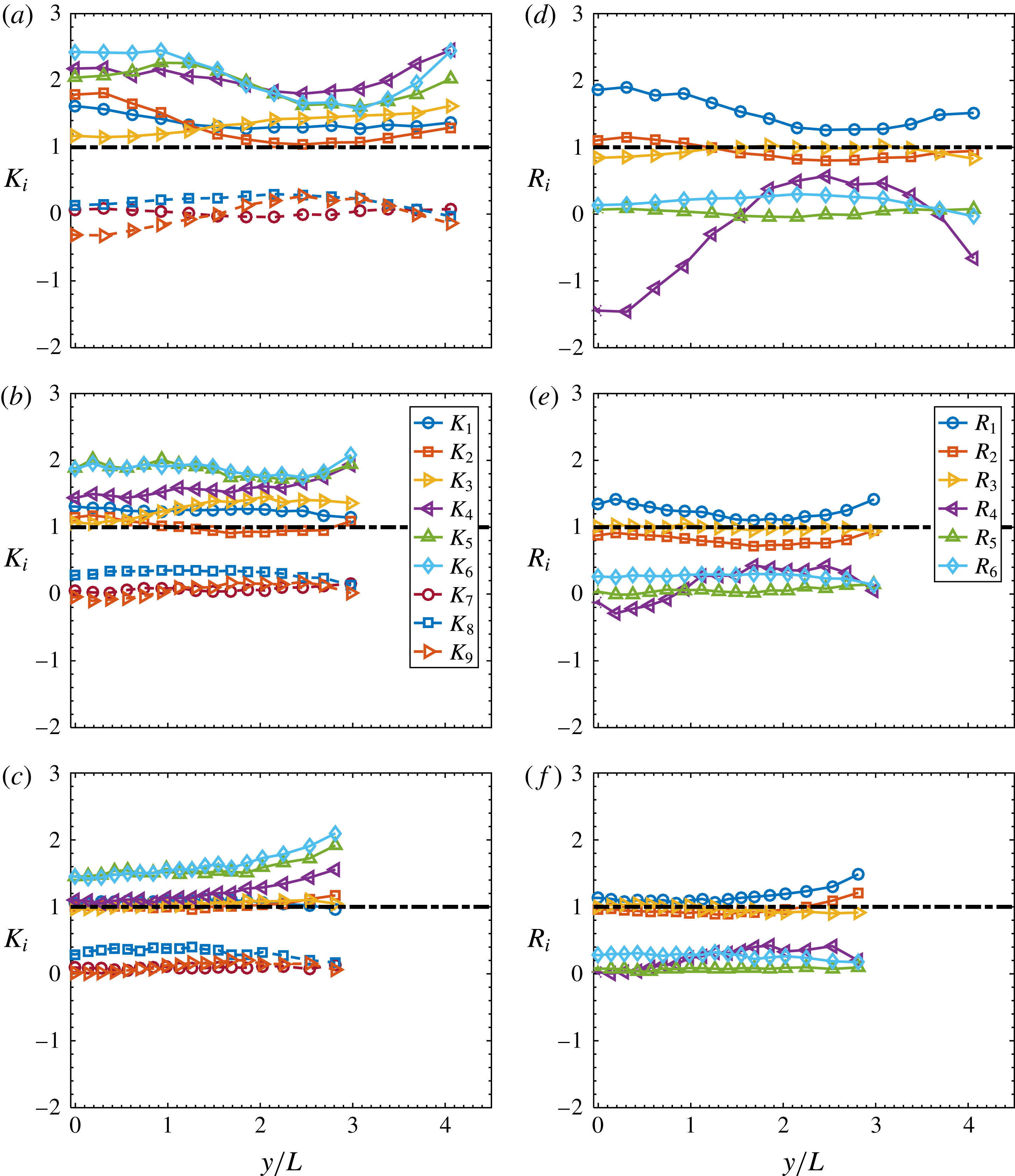
In order to quantify the extent to which both local isotropy and local axisymmetry hold, we have calculated the ratios of the left and right sides of (1.2)–(1.4) (local isotropy) and (1.6)–(1.9) (local axisymmetry). For local isotropy, the ratios are defined by $K_{i}$ , namely

(4.1a-c ) $$\begin{eqnarray}\displaystyle K_{1}=\frac{\overline{2(\unicode[STIX]{x2202}u/\unicode[STIX]{x2202}x)^{2}}}{\overline{(\unicode[STIX]{x2202}v/\unicode[STIX]{x2202}x)^{2}}},\quad K_{2}=\frac{\overline{2(\unicode[STIX]{x2202}u/\unicode[STIX]{x2202}x)^{2}}}{\overline{(\unicode[STIX]{x2202}w/\unicode[STIX]{x2202}x)^{2}}},\quad K_{3}=\frac{\overline{2(\unicode[STIX]{x2202}u/\unicode[STIX]{x2202}x)^{2}}}{\overline{(\unicode[STIX]{x2202}u/\unicode[STIX]{x2202}y)^{2}}}, & & \displaystyle\end{eqnarray}$$

(4.1d-f ) $$\begin{eqnarray}\displaystyle K_{4}=\frac{\overline{2(\unicode[STIX]{x2202}u/\unicode[STIX]{x2202}x)^{2}}}{\overline{(\unicode[STIX]{x2202}u/\unicode[STIX]{x2202}z)^{2}}},\quad K_{5}=\frac{\overline{2(\unicode[STIX]{x2202}u/\unicode[STIX]{x2202}x)^{2}}}{\overline{(\unicode[STIX]{x2202}w/\unicode[STIX]{x2202}y)^{2}}},\quad K_{6}=\frac{\overline{2(\unicode[STIX]{x2202}u/\unicode[STIX]{x2202}x)^{2}}}{\overline{(\unicode[STIX]{x2202}v/\unicode[STIX]{x2202}z)^{2}}}, & & \displaystyle\end{eqnarray}$$

(4.1g-i ) $$\begin{eqnarray}\displaystyle \!\!\!\!\!\!\!\!K_{7}=\frac{\overline{(\unicode[STIX]{x2202}u/\unicode[STIX]{x2202}y)(\unicode[STIX]{x2202}v/\unicode[STIX]{x2202}x)}}{-1/2\overline{(\unicode[STIX]{x2202}u/\unicode[STIX]{x2202}x)^{2}}},\quad K_{8}=\frac{\overline{(\unicode[STIX]{x2202}u/\unicode[STIX]{x2202}z)(\unicode[STIX]{x2202}w/\unicode[STIX]{x2202}x)}}{-1/2\overline{(\unicode[STIX]{x2202}u/\unicode[STIX]{x2202}x)^{2}}},\quad K_{9}=\frac{\overline{(\unicode[STIX]{x2202}v/\unicode[STIX]{x2202}z)(\unicode[STIX]{x2202}w/\unicode[STIX]{x2202}y)}}{-1/2\overline{(\unicode[STIX]{x2202}u/\unicode[STIX]{x2202}x)^{2}}}. & & \displaystyle\end{eqnarray}$$

All these ratios should be unity. For local axisymmetry, the ratios are defined by $R_{i}$ , namely

(4.2a-c ) $$\begin{eqnarray}\displaystyle R_{1}=\frac{\overline{(\unicode[STIX]{x2202}u/\unicode[STIX]{x2202}y)^{2}}}{\overline{(\unicode[STIX]{x2202}u/\unicode[STIX]{x2202}z)^{2}}},\quad R_{2}=\frac{\overline{(\unicode[STIX]{x2202}v/\unicode[STIX]{x2202}x)^{2}}}{\overline{(\unicode[STIX]{x2202}w/\unicode[STIX]{x2202}x)^{2}}},\quad R_{3}=\frac{\overline{(\unicode[STIX]{x2202}v/\unicode[STIX]{x2202}z)^{2}}}{\overline{(\unicode[STIX]{x2202}w/\unicode[STIX]{x2202}y)^{2}}}, & & \displaystyle\end{eqnarray}$$

(4.2d ) $$\begin{eqnarray}\displaystyle R_{4}=\frac{\overline{(\unicode[STIX]{x2202}v/\unicode[STIX]{x2202}z)(\unicode[STIX]{x2202}w/\unicode[STIX]{x2202}y)}}{1/6\overline{(\unicode[STIX]{x2202}u/\unicode[STIX]{x2202}x)^{2}}-1/3\overline{(\unicode[STIX]{x2202}v/\unicode[STIX]{x2202}z)^{2}}}, & & \displaystyle\end{eqnarray}$$

(4.2e,f ) $$\begin{eqnarray}\displaystyle R_{5}=\frac{\overline{(\unicode[STIX]{x2202}u/\unicode[STIX]{x2202}y)(\unicode[STIX]{x2202}v/\unicode[STIX]{x2202}x)}}{-1/2\overline{(\unicode[STIX]{x2202}u/\unicode[STIX]{x2202}x)^{2}}},\quad R_{6}=\frac{\overline{(\unicode[STIX]{x2202}u/\unicode[STIX]{x2202}z)(\unicode[STIX]{x2202}w/\unicode[STIX]{x2202}x)}}{-1/2\overline{(\unicode[STIX]{x2202}u/\unicode[STIX]{x2202}x)^{2}}}. & & \displaystyle\end{eqnarray}$$

All these ratios should be unity. Figure 6 contains the distributions of $K_{i}$ and $R_{i}$ across the wake at the three $x^{\ast }$ positions. As shown in figure 6(a–c), as $x^{\ast }$ increases, $K_{1}$ to $K_{4}$ approach 1, while $K_{7}$ to $K_{9}$ , which are associated with the velocity correlation terms, are quite close to zero because of the small magnitude of the correlation terms compared with that of $-(\overline{(\unicode[STIX]{x2202}u/\unicode[STIX]{x2202}x)^{2}})/2$ (figure 5 a–c). The ratios associated with $\overline{(\unicode[STIX]{x2202}w/\unicode[STIX]{x2202}y)^{2}}$ and $\overline{(\unicode[STIX]{x2202}v/\unicode[STIX]{x2202}z)^{2}}$ , i.e. $K_{5}$ and $K_{6}$ , similarly depart from unity, although the departure decreases from $x^{\ast }=10$ to $x^{\ast }=40$ . It is noted that $K_{1}$ to $K_{6}$ , which are associated with the mean square terms, are generally larger than 1, indicating that the mean energy dissipation rate based on local isotropy can be overestimated in the present flow, especially at $x^{\ast }=10$ and 20, which is confirmed later in figure 9 in § 5 and is also observed by Mi & Antonia (Reference Mi and Antonia2010) and Lefeuvre et al. (Reference Lefeuvre, Thiesset, Djenidi and Antonia2014). On the other hand, as $x^{\ast }$ increases, the ratios $R_{1}$ to $R_{3}$ associated with the mean square terms gradually approach 1, while $R_{4}$ to $R_{6}$ associated with the correlation terms behave similarly to $K_{7}$ to $K_{9}$ , that is, they are nearly zero (figure 6 d–f). Figure 6 indicates that the extent to which both local isotropy and local axisymmetry apply improves downstream for the mean square velocity derivative terms; departures are mainly associated with the velocity derivative correlation terms. Consistent with figure 5, the nearly equal deviation from unity of $K_{5}$ and $K_{6}$ even at $x^{\ast }=40$ (figure 6 c), which is consistent with $R_{3}$ being close to unity (figure 6 f), suggests that the local axisymmetry should be a better description than local isotropy for the velocity derivative variances in the present flow.

Figure 6.

Lateral distributions of ratios $K_{i}$ (4.1a–i ) and $R_{i}$ (4.2a–f ) at (a,d) $x^{\ast }=10$ , (b,e) 20, (c,f) 40. The dash-dotted line in each figure corresponds to unity, which is the locally isotropic value for $K_{i}$ in (a–c) and locally axisymmetric value for $R_{i}$ in (d–f).

It should be recognized that $K_{i}$ and $R_{i}$ provide some qualification of the extent to which local isotropy and local axisymmetry hold. It is also of interest to assess these assumptions in the spectral space in terms of different flow scales. Figure 7 shows the spectra of the seven measured velocity derivatives at the wake centreline. For convenience of comparing spectra of different velocity derivatives, the spectra are normalized to a unity integral with the variance of the corresponding velocity derivative, i.e. $\int _{0}^{\infty }F_{\unicode[STIX]{x2202}u_{i}/\unicode[STIX]{x2202}x_{j}}(k_{1})\,\text{d}k_{1}=\int _{0}^{\infty }E_{\unicode[STIX]{x2202}u_{i}/\unicode[STIX]{x2202}x_{j}}(k_{1})/\overline{(\unicode[STIX]{x2202}u_{i}/\unicode[STIX]{x2202}x_{j})^{2}}\,\text{d}k_{1}=1$ , where $E(k_{1})_{\unicode[STIX]{x2202}u_{1}/\unicode[STIX]{x2202}x_{j}}$ , defined such that $\int _{0}^{\infty }E_{\unicode[STIX]{x2202}u_{i}/\unicode[STIX]{x2202}x_{j}}(k_{1})\,\text{d}k_{1}=\overline{(\unicode[STIX]{x2202}u_{i}/\unicode[STIX]{x2202}x_{j})^{2}}$ , is the power spectral density function of $\unicode[STIX]{x2202}u_{i}/\unicode[STIX]{x2202}x_{j}$ . Similar to the spectra of the energy dissipation rate in figure 2, the spectra in figure 7 are presented in the form of $k_{1}\unicode[STIX]{x1D702}F_{\unicode[STIX]{x2202}u_{i}/\unicode[STIX]{x2202}x_{j}}$ versus $k_{1}\unicode[STIX]{x1D702}$ so that the area under the curve is proportional to the variance of the corresponding velocity derivative.

Figure 7.

Spectral density functions, multiplied by $k_{1}\unicode[STIX]{x1D702}$ , of measured velocity derivatives on the wake centreline at $x^{\ast }=10$ , 20 and 40. The vertical dashed line in each figure denotes the wavenumber corresponding to the vortex shedding frequency.

Several observations can be made from figure 7. Firstly, the Kármán vortices have a profound influence on $\unicode[STIX]{x2202}u/\unicode[STIX]{x2202}y$ and $\unicode[STIX]{x2202}v/\unicode[STIX]{x2202}x$ , compared with the other derivatives. The spectra of both $\unicode[STIX]{x2202}u/\unicode[STIX]{x2202}y$ and $\unicode[STIX]{x2202}v/\unicode[STIX]{x2202}x$ at $x^{\ast }=10$ (figure 7 a) display a pronounced peak at the wavenumber corresponding to $St=0.21$ , which is significantly bigger than that in other spectra at the same wavenumber. The pronounced peak in $F_{\unicode[STIX]{x2202}u/\unicode[STIX]{x2202}y}$ and $F_{\unicode[STIX]{x2202}v/\unicode[STIX]{x2202}x}$ at $St=0.21$ is obviously a footprint of the spanwise vorticity $\unicode[STIX]{x1D714}_{z}$ ( $=\unicode[STIX]{x2202}v/\unicode[STIX]{x2202}x-\unicode[STIX]{x2202}u/\unicode[STIX]{x2202}y$ ), the most organized vorticity component associated with the Kármán vortices in this flow. At $x^{\ast }=20$ (figure 7 b), the pronounced peak in $F_{\unicode[STIX]{x2202}u/\unicode[STIX]{x2202}y}$ or $F_{\unicode[STIX]{x2202}v/\unicode[STIX]{x2202}x}$ at $St=0.21$ contracts but is still much more evident than that in the other spectra. Even at $x^{\ast }=40$ , where the Kármán vortices are quite weak, the peak at $St=0.21$ in $F_{\unicode[STIX]{x2202}u/\unicode[STIX]{x2202}y}$ remains prominent, although the peak in $F_{\unicode[STIX]{x2202}v/\unicode[STIX]{x2202}x}$ is just discernible. Note that a peak occurs at the wavenumber corresponding to $St=0.42$ in the spectrum of $\unicode[STIX]{x2202}w/\unicode[STIX]{x2202}y$ at $x^{\ast }=10$ (figure 7 a), but disappears at $x^{\ast }=20$ and 40. This peak is likely caused by the positive and negative spanwise velocity induced by the rib structures, which are strong and organized even near the wake centreline at $x^{\ast }=10$ but become weak and disordered downstream (Huang, Zhou & Zhou Reference Huang, Zhou and Zhou2006; Djenidi & Antonia Reference Djenidi and Antonia2009; Chen et al. Reference Chen, Zhou, Zhou and Antonia2016).

Secondly, the assumption of local axisymmetry does not necessarily require a collapse in the spectra of the corresponding velocity derivatives on either side of (1.6a–d ). However, it is interesting to see that, as $x^{\ast }$ increases from 10 to 40, the high-wavenumber parts of the spectra gradually collapse into three groups, i.e. $\unicode[STIX]{x2202}u/\unicode[STIX]{x2202}y$ and $\unicode[STIX]{x2202}u/\unicode[STIX]{x2202}z$ , $\unicode[STIX]{x2202}v/\unicode[STIX]{x2202}x$ and $\unicode[STIX]{x2202}w/\unicode[STIX]{x2202}x$ as well as $\unicode[STIX]{x2202}w/\unicode[STIX]{x2202}y$ and $\unicode[STIX]{x2202}v/\unicode[STIX]{x2202}z$ , which correspond to the local axisymmetry assumption, namely (1.6a–c ). In contrast, the agreement between the low-wavenumber parts of the corresponding spectra is not so clear because of the effect of the Kármán vortices ( $St=0.21$ ), especially at $x^{\ast }=10$ and 20. Interestingly, as the pronounced peak in $F_{\unicode[STIX]{x2202}u/\unicode[STIX]{x2202}y}$ and $F_{\unicode[STIX]{x2202}v/\unicode[STIX]{x2202}x}$ at $St=0.21$ gradually retreats from $x^{\ast }=10$ to 40, the high-wavenumber behaviours of $F_{\unicode[STIX]{x2202}u/\unicode[STIX]{x2202}y}$ and $F_{\unicode[STIX]{x2202}v/\unicode[STIX]{x2202}x}$ evolve towards those of $F_{\unicode[STIX]{x2202}u/\unicode[STIX]{x2202}z}$ and $F_{\unicode[STIX]{x2202}w/\unicode[STIX]{x2202}x}$ , respectively, and collapse at $x^{\ast }=40$ . The behaviours at the low and the high wavenumbers of $F_{\unicode[STIX]{x2202}u/\unicode[STIX]{x2202}y}$ and $F_{\unicode[STIX]{x2202}v/\unicode[STIX]{x2202}x}$ suggest that local axisymmetry is first satisfied in the high-wavenumber range, while the departure in the low-wavenumber range is caused by the Kármán-vortex-related motions. It is reasonable to expect that, as the coherent motions weaken further downstream, the agreement between the spectra of the corresponding velocity derivatives should improve in the low-wavenumber range, and local axisymmetry should be better satisfied, as confirmed by Mi & Antonia (Reference Mi and Antonia2010) with the data of Browne et al. (Reference Browne, Antonia and Shah1987) in the self-preserving far wake.

5 Estimation of $\overline{\unicode[STIX]{x1D700}}$ via the spectral chart method

Based on the universality of the dissipative range of the Kolmogorov-normalized longitudinal velocity spectrum, Djenidi & Antonia (Reference Djenidi and Antonia2012) proposed a spectral chart method to estimate the mean energy dissipation rate in various flows where Kolmogorov’s first similarity hypothesis applies. Specifically, the basic procedure is to use ‘guessed’ values of the energy dissipation rate to ‘un-normalize’ a reference universal spectrum iteratively until it collapses onto the measured velocity spectrum over the lower-wavenumber portion of the dissipative range. The focus of this section is to evaluate the spectral chart method to see if it can approximate $\overline{\unicode[STIX]{x1D700}}_{yz}$ in the present flow, notwithstanding the perturbation from the large-scale motions.

Kolmogorov’s first similarity hypothesis, which was enunciated in his well-known paper (Kolmogorov Reference Kolmogorov1941), essentially postulates that the statistics of the small-scale motions (in both the dissipative and inertial ranges) are solely determined by $\overline{\unicode[STIX]{x1D700}}$ and $\unicode[STIX]{x1D708}$ , provided that the Reynolds number is very large and the small scales are isotropic. One implication of this hypothesis is that the dissipation range of the one-dimensional velocity spectrum, normalized by Kolmogorov scales, will collapse onto a universal function of $k^{\ddagger }$ , where ‘ $\ddagger$ ’ denotes normalization by Kolmogorov scales $\unicode[STIX]{x1D702}$ and $u_{K}(\equiv (\unicode[STIX]{x1D708}\overline{\unicode[STIX]{x1D700}})^{1/4})$ . This has been verified through several compilations (e.g. Chapman Reference Chapman1979; Saddoughi & Veeravalli Reference Saddoughi and Veeravalli1994). It should, however, be stressed that Antonia et al. (Reference Antonia, Djenidi and Danaila2014) pointed out that Kolmogorov’s two main requirements, viz. very large Reynolds number and isotropic small-scale structures, can be relaxed, provided the effect of the large scales is negligible. This implies that the first similarity hypothesis may be satisfied in the present flow, where the coherent vortices are present and $Re_{\unicode[STIX]{x1D706}}$ is relatively small (table 1). Figure 8 shows that the spectrum of $u$ scales on $\overline{\unicode[STIX]{x1D700}}_{yz}$ and $\unicode[STIX]{x1D708}$ , both on the centreline ( $y/L=0$ ) and at the location where the shear is large ( $y/L=1$ ). Also included are spectra in the far wake at $x^{\ast }=240$ (Djenidi & Antonia Reference Djenidi and Antonia2012), a turbulent grid flow (Djenidi Reference Djenidi2006) and the centreline of channel flow (Antonia & Abe Reference Antonia and Abe2009). It shows that the velocity spectra at $x^{\ast }=10$ and 40 in the present flow collapse reasonably well onto the other three normalized spectra in the literature which are in conformity with the universal spectrum over sufficiently high wavenumbers (say $k_{1}^{\ddagger }\approx 0.25{-}0.65$ ). The attenuation of the present spectra for $k_{1}^{\ddagger }>0.65$ is due mainly to the imperfect spatial resolution of the probe (Zhu & Antonia Reference Zhu and Antonia1996c ; Zhou et al. Reference Zhou, Antonia, Lasserre, Coantic and Anselmet2003a ).

Figure 8.

Longitudinal velocity spectra normalized by Kolmogorov scales, in which $\overline{\unicode[STIX]{x1D700}}_{yz}$ is used, for $y/L=0$ and $y/L=1$ at $x^{\ast }=10$ and 40, compared with those at the centreline of the far wake ( $R_{\unicode[STIX]{x1D706}}=40$ ), and in DNS grid turbulence ( $R_{\unicode[STIX]{x1D706}}=40$ ) and the centreline of the channel flow ( $R_{\unicode[STIX]{x1D706}}=147$ ).

Figure 9.

Comparison between different surrogates of $\overline{\unicode[STIX]{x1D700}}$ , i.e. $\overline{\unicode[STIX]{x1D700}}_{iso}$ (1.5),  $\overline{\unicode[STIX]{x1D700}}_{a}$ (1.10),  $\overline{\unicode[STIX]{x1D700}}_{hom}$ (1.11),  $\overline{\unicode[STIX]{x1D700}}_{scm}$ estimated using the chart method, and the reference value $\overline{\unicode[STIX]{x1D700}}_{yz}$ (1.12), on the wake centreline at $x^{\ast }=10$ , 20 and 40. Error bars for $x^{\ast }=10$ and 20 are shown.

The reasonable agreement between the velocity spectra of the present flow and those in the literature in the dissipation range bolsters the claim that the spectral chart method is robust, and implies that the application of the method to the present flow seems warranted. A comparison between the mean energy dissipation rate using the spectral chart method and estimates from (1.5), (1.10), (1.11), (1.12) at the centreline are shown in figure 9. The mean energy dissipation rate obtained with the spectral chart method, $\overline{\unicode[STIX]{x1D700}}_{scm}$ , is closer to the reference energy dissipation rate $\overline{\unicode[STIX]{x1D700}}_{yz}$ than the other surrogates of (1.5), (1.10) and (1.11) at the same $x^{\ast }$ . The differences between $\overline{\unicode[STIX]{x1D700}}_{scm}$ and $\overline{\unicode[STIX]{x1D700}}_{yz}$ are approximately 9.3 %, 6.3 %, 2.5 %, respectively, at $x^{\ast }=10$ , 20 and 40, which are satisfactorily small. The relatively larger difference at $x^{\ast }=10$ is reasonable since the anisotropic large-scale motion is stronger there and the measurement attenuation is worse (table 1). Besides, we also have checked that $\overline{\unicode[STIX]{x1D700}}_{yz}$ are 3.9 and 0.40 at $y/L=1$ of $x/d=10$ and 40, respectively, and the corresponding values based on the spectral chart method $\overline{\unicode[STIX]{x1D700}}_{scm}$ are 3.4 and 0.36. The departures between $\overline{\unicode[STIX]{x1D700}}_{scm}$ and $\overline{\unicode[STIX]{x1D700}}_{yz}$ at $y/L=1$ are 13 % and 10 % for $x/d=10$ and 40, respectively. They are larger than the departures between $\overline{\unicode[STIX]{x1D700}}_{scm}$ and $\overline{\unicode[STIX]{x1D700}}_{yz}$ on the centreline (9.3 % and 2.5 % for $x/d=10$ and 40, respectively). This should be due to the effect of the large shear at $y/L=1$ , which causes the flow to be locally more anisotropic than on the centreline. It is interesting to see that the isotropic estimation $\overline{\unicode[STIX]{x1D700}}_{iso}$ always larger than $\overline{\unicode[STIX]{x1D700}}_{yz}$ in the present flow, by 44 %, 25 % and 7 %, respectively, at $x^{\ast }=10$ , 20 and 40, which is in contrast to the far wake, where $\overline{\unicode[STIX]{x1D700}}_{iso}$ always underestimates the total dissipation rate (e.g. Browne et al. Reference Browne, Antonia and Shah1987). The large difference between $\overline{\unicode[STIX]{x1D700}}_{iso}$ and $\overline{\unicode[STIX]{x1D700}}_{yz}$ at $x^{\ast }=10$ and 20 is a reflection of the strong anisotropy there, as is also indicated by the evident scatter in the velocity derivative variances at $x^{\ast }=10$ and 20 in figure 5(a,b). At $x^{\ast }=40$ , the smaller difference between $\overline{\unicode[STIX]{x1D700}}_{iso}$ and $\overline{\unicode[STIX]{x1D700}}_{yz}$ is consistent with the improved agreement among the velocity derivatives (figure 5 c). The difference between the axisymmetric estimate of $\overline{\unicode[STIX]{x1D700}}_{a}$ and $\overline{\unicode[STIX]{x1D700}}_{yz}$ (21 %, 13 %, 7 %) is smaller than that between $\overline{\unicode[STIX]{x1D700}}_{iso}$ and $\overline{\unicode[STIX]{x1D700}}_{yz}$ , which is consistent with the conclusion in § 4 that local axisymmetry is a better descriptor of the small-scale turbulent motions than local isotropy. The $\overline{\unicode[STIX]{x1D700}}_{hom}$ always underestimates $\overline{\unicode[STIX]{x1D700}}_{yz}$ and is the smallest of all the surrogates, which is partly due to the attenuation of the imperfect spatial resolution of the probe. Note that the different surrogates tend to converge towards $\overline{\unicode[STIX]{x1D700}}_{yz}$ as the flow develops downstream and the influence of the coherent motions degrades.

The validity of the spectral chart method in a flow perturbed by coherent motions may seem somewhat surprising. Some additional remarks about the test of Kolmogorov’s first similarity hypothesis seem worthwhile. Although the longitudinal velocity spectra are widely used in the literature to test the hypothesis (see Frisch Reference Frisch1996; Pope Reference Pope2000), presumably because of the ease with which $u$ is measured with a single hot wire, vorticity is more closely associated with small-scale turbulence than velocity (e.g. Antonia et al. Reference Antonia, Shafi and Zhu1996; Chen et al. Reference Chen, Zhou, Antonia and Zhou2017). Antonia et al. (Reference Antonia, Shafi and Zhu1996) found that the shape of the high-wavenumber range of the vorticity spectrum, which appears to be independent of $Re_{\unicode[STIX]{x1D706}}$ , is also compatible with the first similarity hypothesis in the sense it scales uniquely on $\overline{\unicode[STIX]{x1D700}}$ and $\unicode[STIX]{x1D708}$ . They also pointed out that the vorticity spectrum can provide a more sensitive test of the first similarity hypothesis than the velocity spectrum, since the major contribution to the vorticity variance is located at larger wavenumbers than for the velocity variance. The isotropic (also axisymmetric) form of the spectra of the vorticity fluctuations are given by Kim & Antonia (Reference Kim and Antonia1993)

(5.1) $$\begin{eqnarray}\displaystyle & \displaystyle E_{\unicode[STIX]{x1D714}_{x}}(k_{1})=\frac{1}{2}\int _{k_{1}}^{\infty }\frac{E(k)}{k}(k^{2}-k_{1}^{2})\,\text{d}k, & \displaystyle\end{eqnarray}$$

(5.2) $$\begin{eqnarray}\displaystyle & \displaystyle E_{\unicode[STIX]{x1D714}_{y}}(k_{1})=E_{w_{z}}(k_{1})\frac{1}{2}k_{1}^{2}\int _{k_{1}}^{\infty }\frac{E(k)}{k}\,\text{d}k+\frac{1}{4}\int _{k_{1}}^{\infty }\frac{E(k)}{k}(k^{2}-k_{1}^{2})\,\text{d}k, & \displaystyle\end{eqnarray}$$

where $E(k)$ is the three-dimensional energy spectrum and $k$ is the magnitude of the wavenumber vector $\boldsymbol{k}$ . Figure 10 compares the normalized spectra of the three vorticity components on the centreline at $x^{\ast }=10$ and 40 with the DNS spectra (Kim & Antonia Reference Kim and Antonia1993) of $\unicode[STIX]{x1D714}_{x}$ and $\unicode[STIX]{x1D714}_{z}$ on the channel flow centreline. At $x^{\ast }=10$ (figure 10 a), the spectrum of $\unicode[STIX]{x1D714}_{z}$ shows a pronounced peak at the wavenumber corresponding to $St=0.21$ , and deviates from the spectrum of $\unicode[STIX]{x1D714}_{y}$ . None of the three vorticity spectra collapse on the corresponding spectra of the channel flow at high wavenumbers. However, as the Kármán vortex impairs from $x^{\ast }=10$ to 40 (figure 10 b), the peak at $St=0.21$ of $E_{\unicode[STIX]{x1D714}_{z}}(k_{1})^{\ddagger }$ degrades and its high-wavenumber part collapses onto that of $E_{\unicode[STIX]{x1D714}_{y}}(k_{1})^{\ddagger }$ , and both $E_{\unicode[STIX]{x1D714}_{z}}(k_{1})^{\ddagger }$ and $E_{\unicode[STIX]{x1D714}_{y}}(k_{1})^{\ddagger }$ are in good agreement with the DNS spectrum of $\unicode[STIX]{x1D714}_{z}$ of the channel flow at high wavenumbers. There is also good agreement with the DNS spectrum of $\unicode[STIX]{x1D714}_{x}$ for the spectrum $E_{\unicode[STIX]{x1D714}_{x}}(k_{1})^{\ddagger }$ at high wavenumbers. Again, the departures at high wavenumbers is ascribed to the inadequate spatial resolution of the probe, which is more evident than that of the velocity spectra (figure 8). The comparison between measured and DNS vorticity spectra at $x^{\ast }=10$ and 40 suggests that the small-scale similarity is likely to be satisfied only at $x^{\ast }=40$ . This is contrary to the collapse of the velocity spectra both at $x^{\ast }=10$ and 40 shown in figure 8, and supports Antonia et al.’s (Reference Antonia, Shafi and Zhu1996) assertion that vorticity spectra provide a more sensitive test of the first similarity hypothesis than velocity spectra. It also confirms the expectation that large-scale coherent structures indeed have an effect on the small-scale motions at $x^{\ast }=10$ , whereas this effect is quite weak at $x^{\ast }=40$ .

Figure 10.

Comparison between the spectra of the three vorticity components of the present flow on the centreline at $x^{\ast }=10$ and 40, and the spectra of $\unicode[STIX]{x1D714}_{x}$ and $\unicode[STIX]{x1D714}_{z}$ on the centreline of a DNS channel flow from Kim & Antonia (Reference Kim and Antonia1993) ( $R_{\unicode[STIX]{x1D706}}=53$ ).  $\overline{\unicode[STIX]{x1D700}}_{yz}$ is used in the normalization of the present vorticity spectra.

6 Phase-averaged energy dissipation rate and its components

A very distinct feature in the intermediate wake is the dominance of the Kármán vortex street at small $x^{\ast }$ , which is followed by its gradual weakening and eventual disappearance as $x^{\ast }$ increases. It is thus of great interest to investigate the spatial distribution of the turbulent energy dissipation rate as the Kármán vortices evolve through their various stages. Hereinafter, the phase $\unicode[STIX]{x1D719}$ in the isocontour plot (figures 11–13) will be interpreted in terms of a longitudinal distance based on Taylor’s hypothesis, $\unicode[STIX]{x1D719}=0{-}2\unicode[STIX]{x03C0}$ corresponding to the vortex wavelength. The same scale is used for the longitudinal and lateral directions in the contour plots in an effort to minimize any possible distortion in the physical space. The positions of the centres and saddle points, identified from the phase-averaged sectional streamlines (not shown), are marked by ‘ $+$ ’ and ‘ $\times$ ’, respectively. The thick dashed lines give an approximate idea of the boundary of the spanwise vortex, which is approximately 25 % of the maximum value of $|\widetilde{\unicode[STIX]{x1D714}_{z}}|$ (not shown). The inclined dash-dotted line passing through the saddle point represents the diverging separatrix. The flow is left to right.

Figure 11.

Isocontours of phase-averaged $\unicode[STIX]{x2202}u/\unicode[STIX]{x2202}y$ and $\unicode[STIX]{x2202}v/\unicode[STIX]{x2202}x$ variance at $x^{\ast }=10$ : (a) $(\widetilde{\unicode[STIX]{x2202}u/\unicode[STIX]{x2202}y}^{\ast })^{2}$ , contour interval $=$ 0.049; (b) $(\widetilde{\unicode[STIX]{x2202}v/\unicode[STIX]{x2202}x}^{\ast })^{2}$ , contour interval $=$ 0.030.

Figure 12.

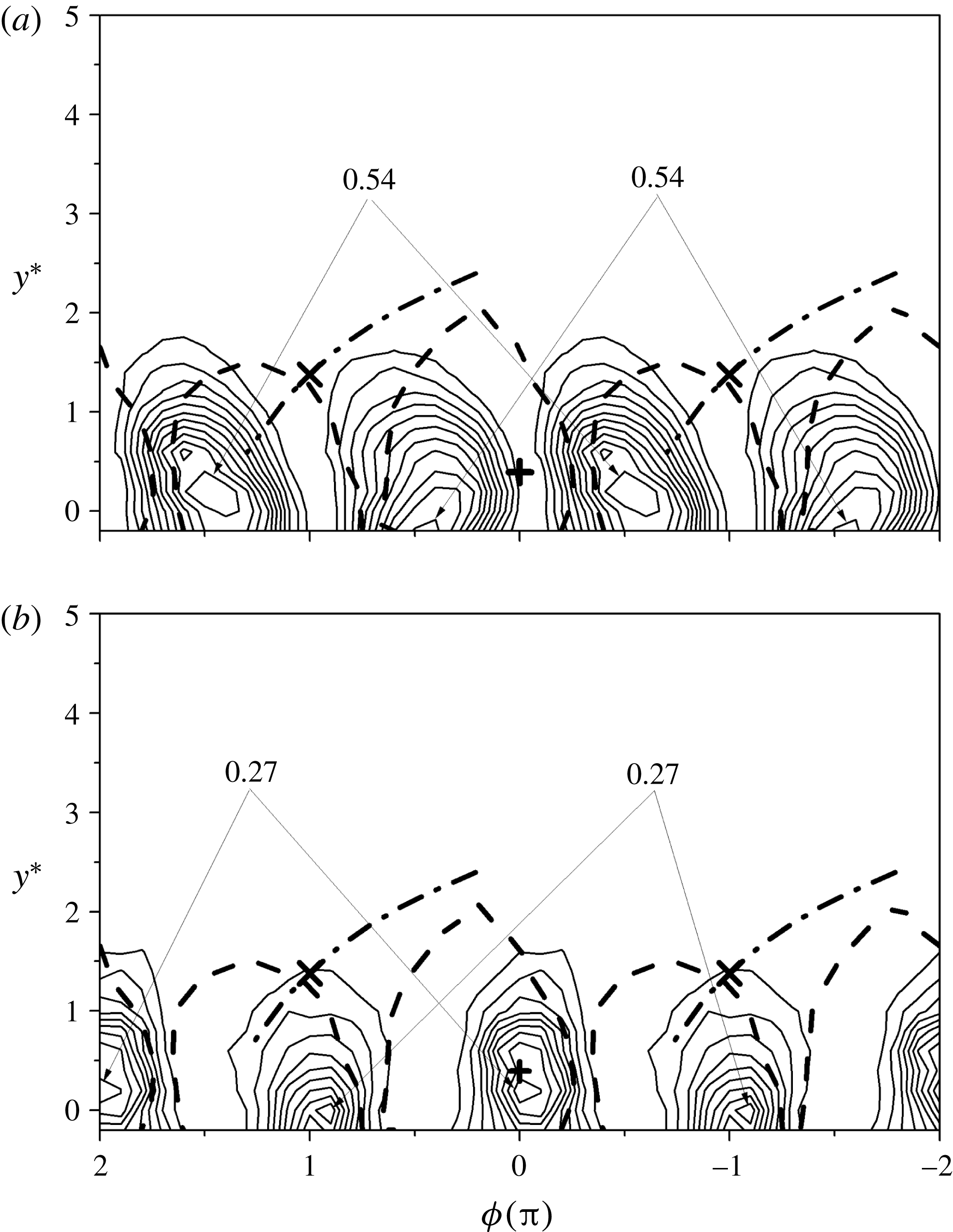
Isocontours of the remainders of the velocity derivatives at $x^{\ast }=10$ . (a) $\langle (\unicode[STIX]{x2202}v/\unicode[STIX]{x2202}x)_{r}^{2}\rangle ^{\ast }$ , contour interval: 0.11; (b) $\langle (\unicode[STIX]{x2202}v/\unicode[STIX]{x2202}z)_{r}^{2}\rangle ^{\ast }$ , contour interval: 0.057; (c) $\langle (\unicode[STIX]{x2202}v/\unicode[STIX]{x2202}y)_{r}^{2}\rangle ^{\ast }$ , contour interval: 0.10; (d) $\langle (\unicode[STIX]{x2202}w/\unicode[STIX]{x2202}x)_{r}^{2}\rangle ^{\ast }$ , contour interval: 0.11; (e) $\langle (\unicode[STIX]{x2202}w/\unicode[STIX]{x2202}y)_{r}^{2}\rangle ^{\ast }$ , contour interval: 0.081; (f) $\langle (\unicode[STIX]{x2202}u/\unicode[STIX]{x2202}z)_{r}^{2}\rangle ^{\ast }$ , contour interval: 0.058.

Figure 13.

Phase-averaged turbulent energy dissipation rate (a–c) $\widetilde{\unicode[STIX]{x1D700}}_{yz}^{\ast }$ and (d–f) the remainder $\langle \unicode[STIX]{x1D700}_{yz,r}\rangle ^{\ast }$ : (a,d) $x^{\ast }=10$ , contour intervals: 0.080, 0.57; (b,e) 20, contour intervals: 0.015, 0.16; (c,f): 40, contour intervals: 0.0028, 0.072.

6.2 Phase-averaged energy dissipation rate

Figure 13 presents the isocontours of the phase-averaged energy dissipation rate and the remainder at all three $x^{\ast }$ positions. The coherent energy dissipation rate (figure 13 a–c) exhibits a distribution similar to that of $(\widetilde{\unicode[STIX]{x2202}u/\unicode[STIX]{x2202}y}^{\ast })^{2}$ (figure 11 a), which makes a dominant contribution to $\widetilde{\unicode[STIX]{x1D700}}_{yz}^{\ast }$ . Actually, the maximum percentage contribution of $(\widetilde{\unicode[STIX]{x2202}u/\unicode[STIX]{x2202}y}^{\ast })^{2}$ to $\widetilde{\unicode[STIX]{x1D700}}_{yz}^{\ast }$ can be as large as almost 80 % near the wake centreline at $x^{\ast }=10$ . On the other hand, the contribution of $(\widetilde{\unicode[STIX]{x2202}v/\unicode[STIX]{x2202}x}^{\ast })^{2}$ to $\widetilde{\unicode[STIX]{x1D700}}_{yz}^{\ast }$ near the vortex centre tends to be cancelled by the negative contribution from $2(\widetilde{\unicode[STIX]{x2202}u/\unicode[STIX]{x2202}y})^{\ast }(\widetilde{\unicode[STIX]{x2202}v/\unicode[STIX]{x2202}x})^{\ast }$ (not shown). The concentrations of the remainder $\langle \unicode[STIX]{x1D700}_{yz,r}\rangle ^{\ast }$ (figure 13 d–f) coincide very well with the Kármán vortex, as the remainders of the velocity derivatives do (figure 12). We have also examined the phase-averaged and remainder isocontours (not shown) of the other three surrogates for the energy dissipation rate (1.5), (1.10) and (1.11). Their concentrations of the remainder are very similar to those of $\langle \unicode[STIX]{x1D700}_{yz,r}\rangle ^{\ast }$ . The maximum concentrations of the coherent energy dissipation rate (figure 13 a–c, 0.72, 0.13, 0.025 at $x^{\ast }=10$ , 20 and 40, respectively) are much smaller than those of the remainder (figure 13 d–f, 6.3, 2.3, 0.49 at $x^{\ast }=10$ , 20 and 40, respectively) at the same $x^{\ast }$ . This is not unexpected, since the energy dissipation occurs primarily at small scales (e.g. Pope Reference Pope2000; Vassilicos Reference Vassilicos2015). It seems that the predominant turbulent energy dissipation takes place within the Kármán vortices, at least for $x^{\ast }\leqslant 20$ . The observation of the remainder energy dissipation rate is consistent with Hussain & Hayakawa’s (Reference Hussain and Hayakawa1987) finding that the incoherent turbulence intensity occurs largely within the Kármán vortex at $x^{\ast }=10$ to 40, and its maximum concentration almost coincides with the Kármán vortex centre. Since the turbulent energy dissipation rate physically reflects the rate at which the turbulent energy is dissipated into heat at small scales, its spatial distribution is expected to be associated with that of the remainder or the smaller-scale turbulent energy. At $x^{\ast }=40$ (figure 13 c,f), the Kármán vortices are quite weak due to vortex interactions and breakup. As a result, both the topologies of the coherent energy dissipation rate and the remainder appear markedly less organized. Nevertheless, the maximum concentration of the remainder remains discernible within the Kármán vortex boundary.

Figure 14.

Coherent contributions ( $\unicode[STIX]{x1D6FC}$ ) to $\overline{(\unicode[STIX]{x2202}u/\unicode[STIX]{x2202}y)^{2}}$ , $\overline{(\unicode[STIX]{x2202}v/\unicode[STIX]{x2202}x)^{2}}$ , and $\overline{\unicode[STIX]{x1D700}}_{yz}$ across the wake at (a) $x^{\ast }=10$ ; (b) 20 and (c) 40.

Figure 15.

(a) Hussain and Hayakawa’s original topological model and (b) the modified model of the flow in a plane wake ( $+$ , vortex centre; $\times$ , saddle point; $\Rightarrow$ engulfed non-turbulent fluid; $==>$ flow of produced turbulence; $A$ : turbulence production; $B_{1}$ and $B_{2}$ : turbulent mixing; $C$ : turbulent kinetic energy dissipation).

6.3 Coherent contribution to the mean energy dissipation rate

The isocontours of $(\widetilde{\unicode[STIX]{x2202}u/\unicode[STIX]{x2202}y}^{\ast })^{2}$ , $(\widetilde{\unicode[STIX]{x2202}v/\unicode[STIX]{x2202}x}^{\ast })^{2}$ (figure 11) and $\widetilde{\unicode[STIX]{x1D700}}_{yz}^{\ast }$ (figure 13) show very well organized structures at $x^{\ast }=10$ which are apparently correlated with the Kármán vortices. Further, the maximum concentration of $(\widetilde{\unicode[STIX]{x2202}u/\unicode[STIX]{x2202}y}^{\ast })^{2}$ and $(\widetilde{\unicode[STIX]{x2202}v/\unicode[STIX]{x2202}x}^{\ast })^{2}$ can be comparable to that of $\langle (\unicode[STIX]{x2202}u/\unicode[STIX]{x2202}y)_{r}^{2}\rangle ^{\ast }$ and $\langle (\unicode[STIX]{x2202}v/\unicode[STIX]{x2202}x)_{r}^{2}\rangle ^{\ast }$ , whereas the concentration of the coherent part of the other velocity derivatives (not shown) is quite small compared to their remainders. The results suggest that the coherent motions make a much larger contribution to $\overline{(\unicode[STIX]{x2202}u/\unicode[STIX]{x2202}y)^{2}}$ and $\overline{(\unicode[STIX]{x2202}v/\unicode[STIX]{x2202}x)^{2}}$ than to the other velocity derivative terms, which intrinsically reflects the way the small scales feel the influence from the large scales associated with the Kármán vortices. The coherent contribution from the coherent motions at a given $y^{\ast }$ position can be quantified by the ratio of the structural average of the phase-averaged coherent quantity to the corresponding Reynolds-averaged quantity (Zhou et al. Reference Zhou, Zhou, Yiu and Chua2003b ), namely

(6.1) $$\begin{eqnarray}\displaystyle \unicode[STIX]{x1D6FC}=\overline{\overline{\widetilde{\unicode[STIX]{x1D6FD}}\widetilde{\unicode[STIX]{x1D6FE}}}}/\overline{\unicode[STIX]{x1D6FD}\unicode[STIX]{x1D6FE}}, & & \displaystyle\end{eqnarray}$$

where $\unicode[STIX]{x1D6FD}$ and $\unicode[STIX]{x1D6FE}$ represent the velocity derivatives $\unicode[STIX]{x2202}u_{i}/\unicode[STIX]{x2202}x_{j}$ as those in §§ 3.1 and 3.2. Figure 14 presents the distribution of $\unicode[STIX]{x1D6FC}$ of $\overline{(\unicode[STIX]{x2202}u/\unicode[STIX]{x2202}y)^{2}}$ and $\overline{(\unicode[STIX]{x2202}v/\unicode[STIX]{x2202}x)^{2}}$ and $\overline{\unicode[STIX]{x1D700}}_{yz}$ across the wake at the three $x^{\ast }$ positions. The coherent contribution to the mean energy dissipation rate, i.e. $\overline{\overline{\widetilde{\unicode[STIX]{x1D700}}_{yz}}}/\overline{\unicode[STIX]{x1D700}}_{yz}$ , is calculated, where $\overline{\overline{\widetilde{\unicode[STIX]{x1D700}}_{yz}}}$ is estimated as the sum of the structural average of all the terms on the right-hand side of (1.12). At $x^{\ast }=10$ (figure 14 a), the coherent contribution accounts for up to 35 % of $\overline{(\unicode[STIX]{x2202}u/\unicode[STIX]{x2202}y)^{2}}$ and 18 % of $\overline{(\unicode[STIX]{x2202}v/\unicode[STIX]{x2202}x)^{2}}$ , respectively, near the centreline. Such large coherent contributions are consistent with the pronounced peak at $St=0.21$ in the spectra of $\unicode[STIX]{x2202}u/\unicode[STIX]{x2202}y$ and $\unicode[STIX]{x2202}v/\unicode[STIX]{x2202}x$ (figure 7 a), as well as the organized structures displayed by $(\widetilde{\unicode[STIX]{x2202}u/\unicode[STIX]{x2202}y}^{\ast })^{2}$ and $(\widetilde{\unicode[STIX]{x2202}v/\unicode[STIX]{x2202}x}^{\ast })^{2}$ (figure 11). The maximum coherent contribution to $\overline{\unicode[STIX]{x1D700}}_{yz}$ is approximately 9 % at $y^{\ast }=0.6$ which corresponds roughly to the lateral location of the maximum concentration of $\widetilde{\unicode[STIX]{x1D700}}_{yz}^{\ast }$ . The relatively small coherent contribution to $\overline{\unicode[STIX]{x1D700}}_{yz}$ , compared with that to $\overline{(\unicode[STIX]{x2202}u/\unicode[STIX]{x2202}y)^{2}}$ and $\overline{(\unicode[STIX]{x2202}v/\unicode[STIX]{x2202}x)^{2}}$ , reflects the very small coherent contributions to the other components of $\overline{\unicode[STIX]{x1D700}}_{yz}$ . The distinct difference between the coherent contribution to $\overline{(\unicode[STIX]{x2202}u/\unicode[STIX]{x2202}y)^{2}}$ and $\overline{(\unicode[STIX]{x2202}v/\unicode[STIX]{x2202}x)^{2}}$ and those to the other velocity derivative terms reflects that the small scales feel the influence from the large scales associated with the Kármán vortices mainly via $\unicode[STIX]{x2202}u/\unicode[STIX]{x2202}y$ and $\unicode[STIX]{x2202}v/\unicode[STIX]{x2202}x$ . The effect of the large-scale motions can still be felt at $x^{\ast }=20$ (figure 14 b), where the maximum coherent contributions to $\overline{(\unicode[STIX]{x2202}u/\unicode[STIX]{x2202}y)^{2}}$ , $\overline{(\unicode[STIX]{x2202}v/\unicode[STIX]{x2202}x)^{2}}$ and $\overline{\unicode[STIX]{x1D700}}_{yz}$ are approximately 15 %, 6 % and 4 %, respectively. Because of the rather weak coherent motions at $x^{\ast }=40$ , the coherent contribution there is negligibly small (figure 14 c).

7 Summary and conclusions

Ten of the twelve terms which make up the mean energy dissipation rate are measured simultaneously with a four X-wire probe at three streamwise locations in a turbulent intermediate wake. Both the statistical and the topological features of the energy dissipation rate as well as its components are examined. Four major conclusions can be drawn from this study.

(1) Local axisymmetry is a better descriptor of the small-scale turbulent motions than local isotropy. The mean square velocity derivative terms satisfy local axisymmetry better than local isotropy. Neither local isotropy nor local axisymmetry are satisfied by the correlation terms. Spectra of velocity derivatives indicate that axisymmetry is first satisfied at high wavenumbers; the departure at low wavenumbers is related to the effect of the Kármán vortices. This effect gradually weakens between $x^{\ast }=10$ and $x^{\ast }=40$ , so that the low-wavenumber part of the spectra begins to satisfy axisymmetry.

(2) The close agreement between $\overline{\unicode[STIX]{x1D700}}_{yz}$ and $\overline{\unicode[STIX]{x1D700}}_{scm}$ estimated via the spectral chart method proposed by Djenidi & Antonia (Reference Djenidi and Antonia2012) indicates that this method, which is based on the collapse, over the dissipative range, of the longitudinal velocity spectrum normalized by Kolmogorov scales, is also applicable for the present flow. $\overline{\unicode[STIX]{x1D700}}_{scm}$ is closer to $\overline{\unicode[STIX]{x1D700}}_{yz}$ than the other three surrogates ( $\overline{\unicode[STIX]{x1D700}}_{iso}$ , $\overline{\unicode[STIX]{x1D700}}_{a}$ , $\overline{\unicode[STIX]{x1D700}}_{hom}$ ) at the same $x^{\ast }$ . It is found that despite the effect of the anisotropic large-scale coherent motions and mean shear at $x^{\ast }=10$ , the dissipative range of the $u$ spectra collapses onto the reference universal spectra in previous studies (figure 8), while the high-wavenumber part of the normalized vorticity spectra only starts to comply with isotropy at $x^{\ast }=40$ . It confirms Antonia et al.’s (Reference Antonia, Djenidi and Danaila2014) observation that the two major assumptions in Kolmogorov’s first similarity hypothesis can be relaxed in the context of the collapse of the spectrum of $u$ in the dissipative range; it also confirms that the vorticity spectrum is a more sensitive test of this hypothesis than the velocity spectrum.

(3) Both $\unicode[STIX]{x2202}u/\unicode[STIX]{x2202}y$ and $\unicode[STIX]{x2202}v/\unicode[STIX]{x2202}x$ play a crucial role in the interaction between large- and small-scale motions in this flow. These velocity derivatives contain mainly information on the small-scale motion since the bulk of their variances is located at high wavenumbers (figure 7). The maximum coherent contribution associated with Kármán vortices to $\overline{(\unicode[STIX]{x2202}u/\unicode[STIX]{x2202}y)^{2}}$ and $\overline{(\unicode[STIX]{x2202}v/\unicode[STIX]{x2202}x)^{2}}$ can be as high as 35 % and 18 %, respectively, near the wake centreline at $x^{\ast }=10$ . This is largely because $\unicode[STIX]{x2202}u/\unicode[STIX]{x2202}y$ and $\unicode[STIX]{x2202}v/\unicode[STIX]{x2202}x$ are associated with the most organized vorticity component $\unicode[STIX]{x1D714}_{z}(=\unicode[STIX]{x2202}v/\unicode[STIX]{x2202}x-\unicode[STIX]{x2202}u/\unicode[STIX]{x2202}y)$ . On the other hand, the coherent contributions to the other velocity derivative variances are almost one order of magnitude smaller than those to $\overline{(\unicode[STIX]{x2202}u/\unicode[STIX]{x2202}y)^{2}}$ and $\overline{(\unicode[STIX]{x2202}v/\unicode[STIX]{x2202}x)^{2}}$ , leading to a quite small coherent contribution (maximum value being approximately 9 % at $x^{\ast }=10$ ) to the total mean energy dissipation rate. Thiesset et al. (Reference Thiesset, Danaila and Antonia2014) found that, close to the wake generator ( $x^{\ast }=10$ ), the influence of the coherent motions can be felt by even the smallest scales. This study further indicates that the coherent motions in the present flow interact with the small-scale turbulent structures mostly via $\unicode[STIX]{x2202}u/\unicode[STIX]{x2202}y$ and $\unicode[STIX]{x2202}v/\unicode[STIX]{x2202}x$ .

(4) Isocontours of the phase-averaged energy dissipation rate $\widetilde{\unicode[STIX]{x1D700}}_{yz}$ are quite similar to those of $(\widetilde{\unicode[STIX]{x2202}u/\unicode[STIX]{x2202}y})^{2}$ , which is the major contributor to $\widetilde{\unicode[STIX]{x1D700}}_{yz}$ . The concentrations of the remainder $\langle \unicode[STIX]{x1D700}_{yz,r}\rangle$ , whose maximum is nearly one order of magnitude larger than that of the coherent concentrations of $\widetilde{\unicode[STIX]{x1D700}}_{yz}$ (figure 13), occur mainly within the Kármán vortices. The same observation applies to the remainder of the other energy dissipation rate surrogates $(\langle \unicode[STIX]{x1D700}_{iso,r}\rangle ,\langle \unicode[STIX]{x1D700}_{a,r}\rangle ,\langle \unicode[STIX]{x1D700}_{hom,r}\rangle )$ . It is therefore concluded that the dominant energy dissipation mainly takes place within the Kármán vortex. A more complete picture for the flow mechanism is proposed by incorporating this information into Hussain & Hayakawa’s (Reference Hussain and Hayakawa1987) model. In the new model, turbulence is produced in the saddle region and is then transported into the vortex structures aligned with the diverging separatrix before being finally dissipated within the Kármán vortex.