2.1. Direct numerical simulations

Before introducing the precise scope of the present study, it is useful to start by briefly examining the effects of APG on the near-wall turbulence in a large computational domain. A direct numerical simulation (DNS) is first employed for plane turbulent Couette flow of a viscous fluid with kinematic viscosity $\nu$ and constant density $\rho$. We denote $x$, $y$, $z$ the streamwise, wall-normal and spanwise directions, respectively, and $u^{\prime }$, $v^{\prime }$, $w^{\prime }$ are the corresponding velocity fluctuations. The flow is assumed to be between two infinitely parallel plates. The lower plate located at $y=-h$ is stationary, whereas the upper plate at $y=h$ moves in the streamwise direction with the speed of $2U_{w}$. Throughout the present study, $Re=2150$ is considered, where $Re=U_wh/ \nu$. The DNS is performed using the numerical solver Diablo (Bewley Reference Bewley2012), which has been extensively verified in previous studies (for further computational detail, see e.g. Yang, Willis & Hwang (Reference Yang, Willis and Hwang2019)).

The computational domain is chosen as $L_x=12h$, $L_y=2h$, $L_z=6h$ with the number of grid points $N_x=128$, $N_y=97$, $N_z=128$ in the streamwise, wall-normal and spanwise directions, respectively. This domain size may not be large enough to accurately capture the large-scale structures in plane Couette flow (Komminaho, Lundbladh & Johansson Reference Komminaho, Lundbladh and Johansson1996; Tsukahara, Kawamura & Shingai Reference Tsukahara, Kawamura and Shingai2006), but it is large enough to study the near-wall dynamics, the main interest of the present study. The one-point turbulence statistics in this domain are found to compare well with those from a DNS with a larger horizontal domain size ($L_x=64h$ and $L_z=12h$). A constant pressure gradient against the streamwise direction is applied, such that the lower part of the channel is exposed to APG, whereas the upper part is subject to a favourable pressure gradient. Several increasing values of the APG $P_{x}(={(h\,{\rm d}\bar p/{{\rm d}\kern0.7pt x})/(\rho U_w^{2}})$, where $\bar {p}$ is the mean pressure) are then considered, until the mean velocity profile near the lower wall exhibits a reverse flow. In this paper three different wall units are used: one, which will be denoted by $(\cdot )^{+}$ is based on the friction velocity of the reference ZPG simulation, whereas the other two are based on the friction velocities at the upper and lower wall, indicated by the subscripts $(\cdot )_u$ and $(\cdot )_l$, respectively. The APG values are in outer units, the reference inner units and the local inner units of the lower wall of each simulation are listed in table 1 with the corresponding friction Reynolds numbers.

Table 1.

The APGs considered for the present DNS with a large computational domain and the corresponding friction Reynolds numbers. Here, $Re_{\tau,l}$ and $Re_{\tau,u}$ are the friction Reynolds numbers based on the friction velocity at the lower and upper wall of each simulation.

2.2. Turbulence statistics

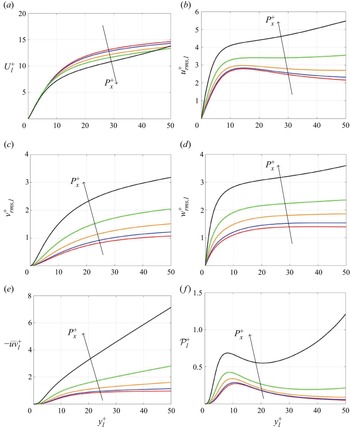
Figure 1 shows for several APG magnitudes the mean velocity profile and other turbulent statistics expressed in the reference wall units based on the friction velocity of the ZPG flow. In these units, in the near-wall region of the lower channel the mean velocity is reduced with increasing APG, leading to a significant reduction of the mean shear in the buffer layer. Despite the difference in flow type, this result is consistent with the previous findings in turbulent boundary layers (Spalart & Watmuff Reference Spalart and Watmuff1993) and is a trivial effect also observed in laminar flows. Figure 1(b–d) show that magnitudes of the components of the velocity fluctuations are also reduced. The Reynolds shear stress and the turbulence production in the buffer layer are reduced significantly (figure 1e, f). Overall, while it is worth noting that for the two largest values of APG there is no peak of the streamwise turbulent intensity and that the reduction trend ceases and is even slightly reversed for wall-normal and spanwise intensities, the observed behaviour might be a natural consequence of the reduced mean shear (figure 1a).

Figure 1.

Turbulent statistics in large computational box of (a) $U^{+}$, (b) $u_{rms}^{+}$, (c) $v_{rms}^{+}$, (d) $w_{rms}^{+}$, (e) $-uv^{+}$, ( f) $\mathcal {P}^{+}$ with $P_{x}^{+}=0.0$ (red), $0.003$ (blue), $0.005$ (orange), $0.007$ (green) $0.009$ (black) at $Re=2150$.

However, the use of the wall units based on the friction velocity at the lower wall of each simulation (figure 2), as it is more appropriate for the analysis of near-wall turbulence, reveals a more complicated picture. Expressed in these units, the mean shear in the near-wall region of the lower channel (figure 2a) is also reduced with increasing APG, even if only by a small amount. In spite of that, the turbulent intensities, Reynolds shear stress and turbulent production are significantly increased, especially in the region far away from the lower wall (figure 2b–f). Note that the extent of anisotropy in the near-wall region is significantly altered by the APG: for example, at $y_l^{+}=10$, $u_{rms,l}^{+}/v_{rms,l}^{+}\approx 6.75$ for $P_{x}^{+}=0.0$, whereas $u_{rms,l}^{+}/v_{rms,l}^{+}\approx 2.75$ for $P_{x}^{+}=0.009$ in figure 2. This suggests that there might be a non-trivial change in the near-wall turbulence due to the increased APG. The analysis of the flow structures and spectra in the following subsection further confirms this observation, and we will subsequently set up the main question to be addressed in the present study.

Figure 2.

Turbulent statistics in large computational box of (a) $U^{+}_{l}$, (b) $u_{rms,l}^{+}$, (c) $v_{rms,l}^{+}$, (d) $w_{rms,l}^{+}$, (e) $-\overline {uv}^{+}_{l}$, ( f) $\mathcal {P}^{+}_{l}$ with $P_{x}^{+}=0.0$ (red), $0.003$ (blue), $0.005$ (orange), $0.007$ (green) $0.009$ (black) at $Re=2150$.

2.3. Flow structures and velocity spectra

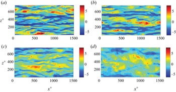
To examine the response of the near-wall streaks to strong APG, instantaneous streamwise velocity fluctuations in the buffer layer are visualised. Near-wall streamwise-elongated streaks are clearly seen in the case of ZPG (figure 3a; note that in figure 3 the same reference wall units are used for all values of the pressure gradient). In the case of a mild and moderate APG, the near-wall streaks still exist, and their structural characteristics are close to those for ZPG (see figure 3b,c). However, strong APG has a significant effect on the strength and the structural characteristics of the near-wall streaks. In particular, comparing figures 3(d) and 3(a) show that if measured in the reference wall units (ZPG wall units), the magnitude of the streamwise velocity fluctuations is significantly reduced by large APG, consistent with figure 1(b).

Figure 3.

Contours of streamwise velocity fluctuation for (a) $P_{x}^{+}=0.0$, (b) $P_{x}^{+}=0.003$, (c) $P_{x}^{+}=0.005$, (d) $P_{x}^{+}=0.009$ at $y^{+}_{l}\approx 10$ away from the lower wall at $Re=2150$.

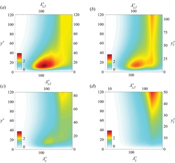
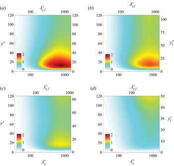
The premultiplied spanwise and streamwise wavenumbers spectra of streamwise velocity normalised by the reference wall units subject to ZPG ($P_{x}^{+}=0.0$), mild APG ($P_{x}^{+}=0.003$), moderate APG ($P_{x}^{+}=0.005$) and strong APG ($P_{x}^{+}=0.009$) are further shown in figures 4 and 5 to support this observation. The APG has a significant impact on the streamwise velocity spectra. Indeed, the strong peaks in figures 4(a) and 5(a) located in the near-wall region of the lower channel are weakened by mild APG and vanish under strong APG (figures 4b–d and 5b–d), consistent with the observation that the near-wall streamwise streaks are suppressed by APG (figure 3). Figures 4 and 5 also reveal the structural characteristics of the streamwise velocity pattern as well. In particular, in the near-wall region of figure 4(a), the local maximum appears at $\lambda _{z,l}^{+}\approx 120$, which agrees with the well known spanwise spacing of the near-wall streaks, and the streamwise wavenumber spectra in figure 5(a) exhibit the typical streamwise length scale of $\lambda _{x,l}^{+}\approx 800$ for the near-wall streaks. For mild and moderate APG, the spanwise wavelength $\lambda _{z}^{+}$ of the near-wall peak is slightly increased in the reference wall units based on the friction velocity under ZPG, with $\lambda _{z,l}^{+}$ still remaining approximately $120$ in wall units based on the lower wall mean friction of the simulation (figure 4b,c). However, for large APG, figures 4(d) and 5(d) show that the spanwise length scale of the near-wall streamwise velocity is increased to $\lambda _{z,l}^{+}\approx 170$, whereas the streamwise length scale is significantly reduced to $\lambda _{x,l}^{+}\approx 300$ in wall units based on the lower wall mean friction of the simulation. In wall units of the reference simulations, these spanwise and streamwise length scales are $\lambda _{z}^{+}\approx 450$ and $\lambda _{x}^{+}\approx 800$, indicating that there is a substantial change in the near-wall dynamics due to the strong APG applied. Importantly, under the strong APG (figures 4d and 5d), the spanwise length scale of the near-wall streamwise velocity structures is similar to that in the centre of the channel, indicating the possible penetration of the outer fluid motions into the near-wall region.

Figure 4.

Premultiplied one-dimensional spanwise wavenumber spectra of streamwise velocity at $Re=2150$: (a) $P_{x}^{+}=0.0$; (b) $P_{x}^{+}=0.003$; (c) $P_{x}^{+}=0.005$; (d) $P_{x}^{+}=0.009$.

Figure 5.

Premultiplied one-dimensional streamwise wavenumber spectra of streamwise velocity at $Re=2150$: (a) $P_{x}^{+}=0.0$; (b) $P_{x}^{+}=0.003$; (c) $P_{x}^{+}=0.005$; (d) $P_{x}^{+}=0.009$.

2.4. Scope of the present study

The observations made in §§ 2.2 and 2.3 raise a non-trivial point about the near-wall dynamics under APG. On the one hand, the characteristic spanwise dimension of the streamwise velocity fluctuations is increased in wall units of the reference ZPG simulation (figures 3d and 4b,c). This could be expected, since such a behaviour follows from the decrease of the mean wall shear by APG and the standard observation that near-wall turbulence, if expressed in terms of the actual friction velocity, is only weakly affected by a pressure gradient. This appears to be true at least when the APG is mild. On the other hand, figures 3 and 4 show that at the same time the streaky pattern, which is a typical feature of near-wall turbulence, almost disappears or is at least completely changed under strong APG, indicating the possible breakdown of the process by which the streaky flow sustains itself. This, too, could be expected because the reduction in the friction velocity caused by APG leads to a decrease in effective Reynolds number in the near-wall region. This can destroy the self-sustaining process, a mean-shear-driven turbulence production mechanism. These two observations draw a consistent picture of near-wall turbulence remaining almost unaffected, when expressed in the pertinent wall units, by a mild pressure gradient, but almost suppressed by strong APG causing a decrease in the effective Reynolds number. However, it is important to note that the near-wall turbulence production under strong APG is not so small compared with that in the channel centre, and they are actually at the same order (see figure 1f). This suggests that there exists a non-trivial near-wall turbulence generation mechanism even under a strong APG possibly in the absence of the self-sustaining process.

The objective of the present study is to answer this question by exploring the effect of APG on the dynamics in the near-wall region in more detail. To simplify the problem, we will continue to consider a turbulent Couette flow with several values of APG. The linear and nonlinear dynamics of the near-wall behaviour of the flow under APG will subsequently be studied using a linear transient growth analysis (Pujals et al. Reference Pujals, García-Villalba, Cossu and Depardon2009; Hwang & Cossu Reference Hwang and Cossu2010a) and the minimal flow unit approach (Jiménez & Moin Reference Jiménez and Moin1991). The analysis shows that the near-wall turbulence production process under strong APG significantly differs from that under ZPG. In particular, here we will propose a new mechanism of near-wall turbulence production under strong APG.

3.1. Linear analysis

To examine how the emergence of the near-wall streaks is affected by APG, a linear analysis based on computation of the optimal perturbation is first performed. Following the previous work (Reynolds & Hussain Reference Reynolds and Hussain1972; Del Alamo & Jimenez Reference Del Alamo and Jimenez2006; Pujals et al. Reference Pujals, García-Villalba, Cossu and Depardon2009; Hwang & Cossu Reference Hwang and Cossu2010a,Reference Hwang and Cossub), we consider the linearised equations for small-amplitude ‘organised’ perturbations, in which the presence of random turbulent fluctuations is modelled with eddy viscosity $\nu _{t}$, i.e.

(3.1a)$$\begin{gather} \boldsymbol{\nabla} \boldsymbol{\cdot} \tilde{\boldsymbol{u}}=0, \end{gather}$$

(3.1b)$$\begin{gather}\frac{\partial \tilde{\boldsymbol{u}}}{\partial t}+ (\boldsymbol{U} \boldsymbol{\cdot}\boldsymbol{\nabla})\tilde{\boldsymbol{u}} + (\tilde{\boldsymbol{u}} \boldsymbol{\cdot}\boldsymbol{\nabla}) \boldsymbol{U} ={-}\frac{1}{\rho} \boldsymbol{\nabla} \tilde{p}+\boldsymbol{\nabla}\boldsymbol{\cdot} [(\nu+\nu_{t})(\boldsymbol{\nabla} \tilde{\boldsymbol{u}}+ \boldsymbol{\nabla} \tilde{\boldsymbol{u}}^{H})], \end{gather}$$

where $\boldsymbol {U}=(U,0,0)$ is the mean velocity, $\tilde {\boldsymbol {u}}=(\tilde {u},\tilde {v},\tilde {w})$ is the perturbation velocity and $\tilde {p}$ is the perturbation pressure. The superscript $(\cdot )^{H}$ indicates a complex conjugate transpose. The streamwise turbulent mean velocity profile $U(y)$ is computed by averaging the instantaneous fields obtained from the DNS in the large computational domain. Once $U(y)$ is obtained, the eddy viscosity is obtained by $\nu _{t}(y)=-\overline {u^{\prime }v^{\prime }}/(\mathrm {d}U/\mathrm {d} y)$, where $\overline {(\cdot )}$ represents averaging over the horizontal plane and in time.

We consider a horizontal Fourier mode of the perturbation velocity, i.e. $\tilde {\boldsymbol {u}}=\hat {\boldsymbol {u}}(y,t)\exp ({{\rm i}(\alpha x+\beta z)})$, where $\alpha$ and $\beta$ are the streamwise and spanwise wavenumbers, respectively. For each Fourier mode, the linear optimal energy growth is obtained from the following optimisation problem:

(3.2)\begin{equation} G(t,\alpha, \beta)=\max_{\hat{{\boldsymbol{u}}}_{0}\not=0} \frac {||{\hat{{\boldsymbol{u}}}}(t)||^{2}}{||{\hat{\boldsymbol{u}}}_{0} ||^{2}}, \end{equation}

where $||\tilde {\boldsymbol {u}}||^{2}= (1/L_y) \int _{-h}^{h} \hat {\boldsymbol {u}}^{H} \hat {\boldsymbol {u}}\,\mathrm {d} y,$ with $\hat {\boldsymbol {u}}_{0}$ representing $\hat {\boldsymbol {u}}$ at $t=0$. The optimisation is performed using the standard method (Schmid & Henningson Reference Schmid and Henningson2001). The Orr–Sommerfeld and Squire system is discretised using the Chebyshev collocation method (Weideman & Reddy Reference Weideman and Reddy2000) with 140 collocation points in the wall-normal direction. The maximum energy growth and the corresponding optimal perturbation are computed by formulating a variational problem, the solution to which is obtained by a singular value decomposition. Once the solution to (3.2) is obtained, the maximum energy growth in time can be further sought by optimising over time, i.e. $G_{max}(\alpha, \beta )=\max _{t}G(t; \alpha, \beta )$. As we shall see below, it is also useful to compute the secondary maximum energy growth $G_{max_{2}}$ to characterise the region near the lower wall. The secondary maximum growth is obtained from the second leading singular value.

It is well known that the near-wall streaks are generated by quasistreamwise vortices via the lift-up mechanism. To understand the effect of APG on the linear generation of near-wall streaks, the linear primary ($G_{max}$) and secondary ($G_{max_{2}}$) maximum energy growth are computed. Figure 6 shows the contours of $G_{max}$ and $G_{max_{2}}$ on the $\alpha \text {--}\beta$ plane under ZPG ($P_{x}^{+}=0.0$) and a strong APG ($P_{x}^{+}=0.009$). As expected, only the streamwise elongated perturbations (i.e. $\beta >\alpha$) can be amplified significantly, and the most amplified ones are streamwise uniform ($\alpha =0$) perturbations for all $\beta$ considered. We note that there is no significant growth for $\beta =0$ and no linear instability is observed, indicating that the Kelvin–Helmholtz mechanism is not active, at least in the cases of the present study, presumably due to the strong confinement posed by the upper and lower walls in the channel. There are two local peaks in the $G_{max}$ contours on the wavenumber plane shown in figure 6(a), one at $\beta h \approx 1.3$ ($\lambda _z/h\approx 4.8$) and the other at $\beta h \approx 9.7$ ($\lambda _{z,l}^{+}\approx 80$). The former indicates the linear growth for the large-scale streaky structures, while the latter is associated with the near-wall streaks (Hwang & Cossu Reference Hwang and Cossu2010a). We note that having two walls in plane Couette flow (i.e. upper and lower walls) implies that there must be two different modes which retain the same maximum transient growth (see also Hwang & Cossu (Reference Hwang and Cossu2010b)). This is seen in figure 6(b) where the contours of $G_{max_2}$ are shown under ZPG. The secondary maximum corresponds to the perturbation containing only near-wall streaks.

Figure 6.

Contour of optimal transient growth as a function of the streamwise and spanwise wavenumbers for (a,b) $P_{x}^{+}=0.0$ and (c,d) $P_{x}^{+}=0.009$ with (a,c) $G_{max}$ and (b,d) $G_{max_{2}}$. The blue dashed lines represent (a,b) $\lambda _{z}^{+}=80$, (c) $\lambda _{z,u}^{+}=80$ and (d) $\lambda _{z,l}^{+}=160$.

We now consider $G_{max}$ and $G_{max_{2}}$ under the action of a strong APG. Comparing figure 6(a) with figure 6(c) shows that the maximum energy growth $G_{max}$ at small $\beta$ (i.e. the peak corresponding to large-scale structures) is not so different for the two cases, suggesting that the effect of a strong pressure gradient on the linear amplification for large-scale motions is modest. This does not appear to be consistent with the previous findings in turbulent boundary layers subject to APG (see § 1), but this is presumably due to the different flow configuration of the present study that is expected to affect the large-scale structure dynamics non-negligibly. It can also be seen from this comparison that $G_{max}$ for large $\beta$ (i.e. the peak corresponding to small-scale structures with $\lambda _{z,u}^{+}\approx 80$) is less pronounced at strong APG. This is presumably due to the increased separation between large outer and viscous inner scales at the upper wall region (i.e. the increase of the related friction Reynolds number; see table 1) at low $Re_{\tau }$ in the present study, as was observed previously in Hwang & Cossu (Reference Hwang and Cossu2010b) for $Re_\tau \lesssim 500$. Figure 6(d) shows that the secondary maximum energy growth $G_{max_{2}}$ is significantly damped by the strong APG (compare with figure 6c). The pressure gradient strongly affects the structural characteristics of the optimal perturbation for $G_{max_{2}}$ as well. In particular, under the strong APG, the maximum of $G_{max_{2}}$ appears at $\beta h \approx 2.1$ ($\lambda _z/h\approx 3$), which is close to that of the large-scale optimal perturbation for $G_{max}$ in outer units (figure 6c,d). In wall units based on the friction velocity at the lower wall, the related spanwise wavelength is $\lambda _{z,l}^{+}\approx 150$, consistent with the near-wall peak location in the premultiplied spectra from DNS in § 2.3.

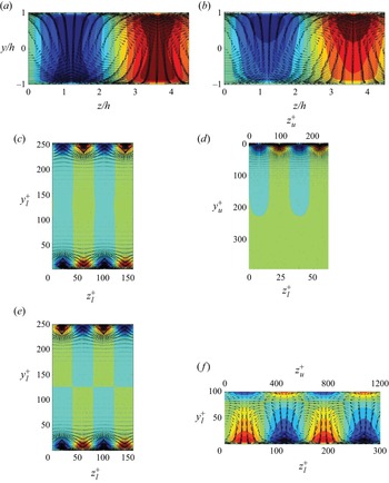
Figure 7 shows the optimal initial conditions and the corresponding responses associated with the local peaks for the $G_{max}$ and $G_{max_{2}}$ in figure 6. In the case of ZPG, it has been well understood that most of the energy initially lies in the cross-stream components in the form of counter-rotating streamwise vortices. The large-scale streamwise streaky motions are subsequently generated via the lift-up effect (figure 7a). Under strong APG, the large-scale optimal perturbation in the form of counter-rotating streamwise vortices still appears across the entire channel at the initial time instant, but the symmetry about the channel centre becomes broken (figure 7b). In particular, it is seen that the generated large-scale streaky motions in the lower half of the channel are much weaker than those in the upper half. This is evidently a consequence of the significant reduction in the mean shear in the lower half of the channel by strong APG.

Figure 7.

Cross-stream view of the optimal perturbation for (a,c,e) $P_{x}^{+}=0.0$, (b,d, f) $P_{x}^{+}=0.009$. All the optimal perturbations here are streamwise uniform (i.e. $\alpha =0$). The spanwise wavenumbers are (a,b) $\beta h =1.3$ ($\lambda _z/h=4.83$), (c,e) $\beta _l^{+}=0.08$ ($\lambda _{z,l}^{+}=81.68$), (d) $\beta _u^{+}=0.05$ ($\lambda _{z,u}^{+}=118.84$) and (f)  $\beta _l^{+}=0.04$ ($\lambda _{z,l}^{+}=153.49$). The red and blue contours denote the positive and negative values of the streamwise velocity with increment of 0.2 of the maximum at $t_{opt}$. The cross-stream velocity components are represented by vectors at $t=0$.

The small-scale optimal perturbation for $G_{max}$ with ZPG appears in the near-wall region of both lower and upper channels, and it is (even) symmetric about the channel centre (figure 7c). For ZPG, the values of $G_{max}$ and $G_{max_2}$ are the same, as shown in figure 7(a,b). In this case, the optimal initial condition and its response for the local peak of $G_{max_{2}}$ are also similar to those for the one of $G_{max}$. However, in this case, they exhibit an odd symmetry about the middle of the channel.

When a strong APG is applied, the small-scale optimal perturbation for $G_{max}$ shown in figure 7(d) is only located in the near-wall region of the upper channel. Therefore, the related peak of $G_{max}$ is expected to scale well, when normalised by the inner units of the upper wall. Therefore, figure 7(d) is plotted by scaling with the inner units of the upper wall, and this is consistent with the emergence of the small-scale peak for $G_{max}$ under strong pressure gradient around $\lambda _{z,u}^{+} \simeq 80$. On the other hand, in the presence of APG, the small-scale optimal perturbation for $G_{max_2}$, responsible for the local peak in figure 6(d), is mainly located in the lower channel, as shown in figure 7( f). We again note that this perturbation experiences a fairly weak linear energy growth (see figure 6d), explaining the disappearance of near-wall streamwise streaks for strong APG observed in § 2.3.

3.2. Self-sustaining process in the presence of APG

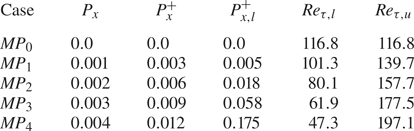
To study the processes beyond the linear dynamics of the streaks in the near-wall region subject to APG, the minimal flow units (Jiménez & Moin Reference Jiménez and Moin1991; Hamilton et al. Reference Hamilton, Kim and Waleffe1995) are considered for the different pressure gradients. In particular, the computational domain size of each case is adjusted to maintain $L_{x,l}^{+}\times L_{z,l}^{+} \approx 250 \times 125$, such that the developed turbulence can contain a single low-speed (or high-speed) streak and the related quasistreamwise vortices in the near-wall region of the lower channel. In table 2, the pressure gradients considered and the resulting friction Reynolds numbers are listed. For all the simulations, $Re=2150$ as was considered in § 2. Here, it should be mentioned that the near-wall statistics and dynamics in the minimal flow unit of plane Couette flow are unchanged with Reynolds numbers, if $Re_\tau \gtrsim 100$. This is basically due to the fact that the inner-scaled equations for the mean and turbulent fluctuations are not a function of $Re_\tau$. Indeed, it was recently shown by Doohan et al. (Reference Doohan, Willis and Hwang2019) that the near-wall turbulence statistics and spectra of the minimal flow unit in Couette flow at $Re_\tau \simeq 73$ are identical to those obtained by simulating the equations for near-wall turbulence in the limit of $Re_\tau \rightarrow \infty$. Therefore, it is expected that the near-wall dynamics studied here would be fairly general, at least for parallel wall-bounded shear flows.

Table 2.

The APGs considered for the present DNS with the minimal flow unit and the corresponding friction Reynolds numbers. Here, $Re_{\tau,l}$ and $Re_{\tau,u}$ are the friction Reynolds numbers normalised by the friction velocity at the lower and upper wall of each simulation.

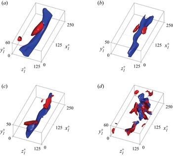
Figure 8 shows the flow visualisation of streamwise and wall-normal velocity fluctuations for ZPG ($P_{x}^{+}=0.0$), mild APG ($P_{x}^{+}=0.003$), moderate APG ($P_{x}^{+}=0.006$) and strong APG ($P_{x}^{+}=0.012$) at the time instant when the streamwise turbulent kinetic energy in the region near the lower wall achieves its local maximum (here, the streamwise turbulent kinetic energy in the region near the lower wall is defined as $E_{u}= (1/ (2V_{n})) \int _{\varOmega } {u^{\prime }}^{2} \,\mathrm {d}V$ where $\varOmega$ represents the computational domain for $y_l^{+} \in [0,50]$ and $V_{n}$ is the volume of $\varOmega$). The visualisation of the flow field for ZPG, mild APG and moderate APG are similar to each other, where there clearly exists a strong near-wall streak extending over the entire streamwise domain with some wall-normal velocity structures representing streamwise vortices (figure 8a–c). In addition, the structural characteristics of the streamwise streaks under mild and moderate APG are close to those with ZPG, consistent with the observations in the large computational domain. However, for strong APG, the flow field no longer exhibits the highly anisotropic feature of the near-wall turbulence (i.e. the streamwise elongated streaks), even when $E_{u}$ reaches its local peak (figure 8d). In addition, both the streamwise and wall-normal velocity structures appear to be highly collocated in the computational domain, and the wall-normal velocity structures are also quite intense, unlike those for ZPG.

Figure 8.

The three-dimensional flow visualisation with (a) $P_{x}^{+}=0.0$ of $u^{+}_{l}=-4.1$, $v^{+}_{l}=1.9$, (b) $P_{x}^{+}=0.003$ of $u^{+}_{l}=-4.8$, $v^{+}_{l}=2.7$, (c) $P_{x}^{+}=0.006$ of $u^{+}_{l}=-6.0$, $v^{+}_{l}=3.3$ and (d) $P_{x}^{+}=0.012$ of $u^{+}_{l}=-8.9$, $v^{+}_{l}=5.6$ at the time instant when streamwise kinetic energy reaches the local peak at $Re=2150$. The blue and red isosurfaces represent the streamwise and wall-normal velocity fluctuations in wall units based on the lower wall, respectively.

To further examine the observation in figure 8, the observables, which represent the kinetic energies of the key structural elements for the self-sustaining process (i.e. straight streaks, wavy streaks, straight rolls and wavy rolls), are defined as

(3.3a)$$\begin{gather} E_{ss}(t) =\tfrac{1}{2} \langle \langle u^{\prime} \rangle_{x}^{2} \rangle_{y,z}, \end{gather}$$

(3.3b)$$\begin{gather}E_{ws}(t) =\tfrac{1}{2} \langle( u^{\prime}- \langle u^{\prime} \rangle_{x})^{2} \rangle_{y,z}, \end{gather}$$

(3.3c)$$\begin{gather}E_{sr}(t) =\tfrac{1}{2} \langle \langle v^{\prime} \rangle_{x}^{2} + \langle w^{\prime} \rangle_{x}^{2} \rangle_{y,z}, \end{gather}$$

(3.3d)$$\begin{gather}E_{wr}(t) =\tfrac{1}{2} \langle( v^{\prime}- \langle v^{\prime} \rangle_{x})^{2} + ( w^{\prime}- \langle w^{\prime} \rangle_{x})^{2} \rangle_{y,z}, \end{gather}$$

where $\langle \cdot \rangle _{x}$ indicates the average in the streamwise direction, $\langle \cdot \rangle _{y,z}$ represents the average in the spanwise direction and $y_l^{+} \in [0,50]$ (Doohan et al. Reference Doohan, Willis and Hwang2019, Reference Doohan, Willis and Hwang2021). Here, we note that all the observables are normalised by the inner units of the lower wall, because the mean shear, the ultimate source of turbulence production, scales well in these units (see figure 2a).

Figure 9 shows the time traces of $E_{ss,l}^{+}$, $E_{ws,l}^{+}$, $E_{sr,l}^{+}$ and $E_{wr,l}^{+}$ for ZPG, mild, moderate and strong APG. Here, the relevant time scale is chosen from the inner units of the lower-wall region, because it characterises the related mean shear (see figure 2a). For ZPG, $E_{ss,l}^{+}$ is much greater than the others (figure 9a), suggesting that the largest amount of the turbulent kinetic energy is contained in the streamwise elongated streaks. There is also a clear phase difference between the oscillations of $E_{ss,l}^{+}$ and the other three variables. In particular, $E_{ws,l}^{+}$ and $E_{wr,l}^{+}$ reach their local peaks when $E_{ss,l}^{+}$ is small, indicating the ‘wavy’ streaks and rolls are generated when the streaks are broken down. All these observations are consistent with the existence of the self-sustaining process in the near-wall region of the lower channel for ZPG. For mild and moderate APG, ‘wavy’ streaks and rolls become relatively stronger than those under ZPG, despite that the largest amount of kinetic energy is still contained in ‘straight’ streaks (figure 9b,c). In contrast, for strong APG (figure 9d), the kinetic energy of wavy rolls $E_{wr,l}^{+}$ is predominant, indicating that the coherent structures here contain highly energetic streamwise-dependent vortical motions. This is consistent with the observations on the turbulent intensities in the large computational domain in § 2.2 and the flow visualisation in minimal flow units in § 3.2, suggesting that the streamwise elongated streaks are no more the main flow feature under strong APG. In addition, the time scales of all four observables with strong APG become much smaller than those with ZPG. The phase difference between them is not obvious either, as all the observables in (3.3) appear to reach their local peaks almost simultaneously.

Figure 9.

Time traces of the energetic terms $E_{ss,l}^{+}$ (red), $E_{ws,l}^{+}$ (blue), $E_{sr,l}^{+}$ (green), $E_{wr,l}^{+}$ (black) with (a) $P_{x}^{+}=0.0$, (b) $P_{x}^{+}=0.003$, (c) $P_{x}^{+}=0.006$, (d) $P_{x}^{+}=0.012$ in the local wall units based on the friction velocity of the lower wall averaged in the near-wall region of the lower channel at $Re=2150$.

For a more quantitative analysis of the time evolution of the four observables, the temporal autocorrelations and cross-correlations of $E_{ss,l}^{+}$, $E_{ws,l}^{+}$, $E_{sr,l}^{+}$ and $E_{wr,l}^{+}$ are further computed. The correlation functions are defined as

(3.4)\begin{equation} C(\tau)=\frac{\left \langle A(t+\tau)B(t) \right \rangle} {\sqrt{\left \langle A^{2}(t) \right \rangle} \sqrt{\left \langle B^{2}(t) \right \rangle}}, \end{equation}

where $A$ and $B$ are the observables defined in (3.3) and $\langle \cdot \rangle$ represents the average in time. Figures 10(a) and Figure 10(b) show the autocorrelation functions of $E_{ss,l}^{+}$ and $E_{ws,l}^{+}$ for ZPG, mild, moderate and strong APG. Again, the correlation functions are scaled by inner units of the lower wall. The reason of choosing this scaling is that the inner units of the lower wall would approximate the properties from the mean shear in the near lower wall region, i.e. the source of turbulence production. However, we do not expect that the correlation functions would scale well in the inner units, as the physical processes of turbulence generation for ZPG appear to be very different from those for strong APG (see also figures 12 and 14). The autocorrelations of the two observables confirm that their temporal oscillations with strong APG take place over a time scale much shorter than those with ZPG, when expressed in inner units of the lower wall for each simulation. The cross-correlations between $E_{ss,l}^{+}$ and $E_{ws,l}^{+}$ and between $E_{sr,l}^{+}$ and $E_{ss,l}^{+}$ are also shown in figures 10(c) and Figure 10(d). For ZPG, the peak correlation between $E_{ss,l}^{+}$ and $E_{ws,l}^{+}$ is clearly shifted to the left, suggesting that the straight streaks appear before the wavy streaks become active, consistent with the streak instability and breakdown in the self-sustaining process. The correlation between $E_{sr,l}^{+}$ and $E_{ss,l}^{+}$ has a slightly left-shifted peak, but it exhibits a large correlation over a quite long time scale. This suggests that the straight streaks are initiated by the straight rolls, and they stay together for a sufficiently long time in a correlated manner, indicative of the lift-up effect. The two cross-correlations also suggest that the three observables are active in the sequence of $E_{sr,l}^{+} \rightarrow E_{ss,l}^{+} \rightarrow E_{ws,l}^{+}$, consistent with the typical casual relation in the self-sustaining process (Hamilton et al. Reference Hamilton, Kim and Waleffe1995; Hwang & Bengana Reference Hwang and Bengana2016). However, with mild and moderate APG, the peak correlation between $E_{ss,l}^{+}$ and $E_{ws,l}^{+}$ is moved in the right-hand direction, and the time scale of the large correlation between $E_{sr,l}^{+}$ and $E_{ss,l}^{+}$ is gradually reduced. For strong APG, this casual relation in the self-sustaining process becomes much less clear. In particular, the cross-correlation between $E_{ss,l}^{+}$ and $E_{ws,l}^{+}$ becomes more positively correlated at $\tau ^{+}_l=0$ with a much shorter correlation time scale (figure 10c). Also, the correlation between $E_{sr,l}^{+}$ and $E_{ss,l}^{+}$ for strong APG does not exhibit a long tail for $\tau ^{+}_l>0$ unlike that for ZPG (figure 10d).

Figure 10.

Temporal autocorrelation function of (a) $E_{ss,l}^{+}$ and (b) $E_{ws,l}^{+}$. Temporal cross-correlation function of (c) $E_{ss,l}^{+}$ and $E_{ws,l}^{+}$, (d) $E_{sr,l}^{+}$ and $E_{ss,l}^{+}$ for $P_{x}^{+}=0.0$ (red lines), $P_{x}^{+}=0.003$ (blues lines), $P_{x}^{+}=0.006$ (orange lines) and $P_{x}^{+}=0.012$ (black lines) at $Re=2150$.

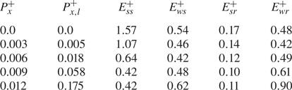
The observations with figures 9 and 10 suggest that the near-wall self-sustaining process is presumably destructed or at least significantly altered by strong APG. This becomes more evident when the observables are expressed in the inner units of the reference ZPG simulation. Table 3 shows the time-averaged $E_{ss}$, $E_{ws}$, $E_{sr}$ and $E_{wr}$ for several values of $P_{x}^{+}$ in wall units of the reference ZPG simulation. It is seen that $E_{ss}^{+}$ is decreased in reference wall units (or outer units equivalently), as the applied APG is gradually increased (table 3). This is consistent with the previous observations for strong APG, suggesting the disappearance of the near-wall streaks, a key structural element in the self-sustaining process. Table 3 also suggests that the typical features observed with the self-sustaining process (e.g. high value of $E_{ss}^{+}>E_{wr}^{+}$) disappear at sufficiently high APG (say $P_{x}^{+} \gtrsim 0.007$). Indeed, for $P_{x}^{+} \lesssim 0.006$, it would still be difficult to argue that the self-sustaining process is destroyed by APG, especially given the strong energy in the straight streaks (i.e. $E_{ss}^{+}$). For such a mild APG, it was previously proposed that the streak instability/breakdown processes are altered, such that the varicose mode streak instability (i.e. streak thickness variation) becomes dominant over the sinuous mode streak instability (i.e. streak meandering motion) (Marquillie et al. Reference Marquillie, Ehrenstein and Laval2011). In the remainder of this subsection, we will investigate this issue.

Table 3.

Time-averaged values of $E_{ss}$, $E_{ws}$, $E_{sr}$ and $E_{wr}$ in inner units of the reference ZPG simulation.

For the purpose of studying how the streak instability/breakdown process is affected by APG, the following productions from the streamwise independent (or streaky) flow are introduced (Park & Huerre Reference Park and Huerre1995):

(3.5a,b)\begin{equation} T_{y}={-}\int_{\varOmega} \check{u} \check{v} \frac{\partial{{U}_s}}{\partial{y}}\,\mathrm{d}V,\quad T_{z}={-}\int_{\varOmega} \check{u} \check{w} \frac{\partial{{U}_s}}{\partial{z}}\,\mathrm{d}V, \end{equation}

where ${\check {\boldsymbol {u}}}(=(\check {{u}},\check {{v}},\check {{w}}))=\boldsymbol {u^{\prime }}-\langle \boldsymbol {u^{\prime }} \rangle _x$ and $U_s(y,z)=U(y)+\langle {u^{\prime }} \rangle _x$. Here, $\varOmega$ is the flow domain for $y_l^{+}\in [0,50]$. The term $T_{y}$ is the production by wall-normal mean shear representing the activation of the varicose mode of the streak instability and/or transient growth, whereas the term $T_{z}$ is the production by spanwise mean shear indicating the sinuous mode instability.

Figure 11 shows the time evolution of $T_{y,l}^{+}$ and $T_{z,l}^{+}$ in the near-wall region of the lower channel under ZPG and strong APG. Under ZPG, $T_{z,l}^{+}$ is much greater than $T_{y,l}^{+}$ (figure 11a). This implies that the streak breakdown primarily takes place via a sinuous mode instability, as was observed in previous studies for turbulent Couette flow (Hamilton et al. Reference Hamilton, Kim and Waleffe1995) and turbulent channel flow (Schoppa & Hussain Reference Schoppa and Hussain2002; Cassinelli et al. Reference Cassinelli, de Giovanetti and Hwang2017). For strong APG, (figure 11b), the ratio of the magnitude of $T_{y,l}^{+}$ to the magnitude of $T_{z,l}^{+}$ appears to be greater, indicating possibly an increased role of the varicose mode instability in the breakdown process. 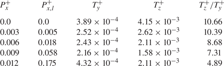The time-averaged values of $T_{y}^{+}$ and $T_{z}^{+}$ for several different values of APG are further shown in table 4. As the APG increases, the ratio of mean values of $T_{z}^{+}$ and $T_{y}^{+}$ consistently decreases. This supports the notion that APG increases the role of the wall-normal shear in the streak instability and breakdown process. The observation here is consistent with the previous analysis of Marquillie et al. (Reference Marquillie, Ehrenstein and Laval2011) in a converging–diverging channel, where the coexistence of the sinuous and varicose instability modes was reported for relatively small APG (i.e. their upper wall region). However, the varicose-mode dominant feature for strong APG in their study (i.e. their lower wall region) is not observed here. This is possibly because the values of APG in the present study ($P_{x,l}^{+} \leqslant 0.175$) are smaller than those in Marquillie et al. (Reference Marquillie, Ehrenstein and Laval2011) ($P_{x,l}^{+}>0.2$). Furthermore, it should also be mentioned that the APG zone in their study emerges in a spatially varying manner due to their converging–diverging channel, whereas, in the present study, the flow is statistically perfectly parallel. Therefore, this difference suggests that the strongly non-parallel nature of the flow in Marquillie et al. (Reference Marquillie, Ehrenstein and Laval2011) with a stronger APG may also be related to the emergence of the varicose mode instability.

Figure 11.

Time traces of $T_{y,l}^{+}$ (red), $T_{z,l}^{+}$ (blue) with (a) $P_{x}^{+}=0.0$, (b) $P_{x}^{+}=0.012$ in local inner units of the lower wall at $Re=2150$.

Table 4.

Time-averaged $T_y^{+}$, $T_z^{+}$ and their ratio $T_{z}^{+}/T_{y}^{+}$ in the near-wall region of the lower channel for several values of APG.

3.3. Turbulence production under strong APG

When the applied APG is strong enough ($P_{x}^{+} \gtrsim 0.007$), the flow features observed in table 3 (e.g. absence of streamwise elongated streaks) no longer indicate the presence of the self-sustaining process in the near-wall region of the lower channel. Nevertheless, the near-wall region still exhibits non-zero velocity fluctuations and turbulence production. We will investigate the origin of a turbulence production mechanism using conditional averaging.

Instantaneous turbulent production averaged in the near-lower-wall region is defined as

(3.6)\begin{equation} \mathcal{P}_{\varOmega}(t)=\int_{\varOmega} -u^{\prime}v^{\prime} \frac{\partial{U}}{\partial{y}}\,\mathrm{d}V, \end{equation}

where $\varOmega$ is defined as before. The time instants (say $t=t_{max}$), at which $\mathcal {P}_{\varOmega }(t)$ reaches local maximal, are then collected, when $\mathcal {P}_{\varOmega,l}^{+}(t)$ is greater than a certain threshold value $P_{th,l}^{+}$, i.e. $\mathcal {P}_{\varOmega,l}^{+}(t)>P_{th,l}^{+}$ where $P_{th,l}^{+}$ was chosen to be 1.2 (see also figure 16b for this choice). At each $t_{max}$, the horizontal location ($x_{max}$,$z_{max}$), where the velocity field retains the maximum value of the integrand in (3.6), is then sought. Finally, the following conditional averaging is computed:

(3.7)\begin{equation} \boldsymbol{u}^{\prime}_{c} (\Delta x,y,\Delta z,\Delta t) = \frac{1}{N} \sum_{n=1}^{N}\boldsymbol{u}^{\prime}_{n}(\Delta x,y,\Delta z,\Delta t), \end{equation}

where $(\Delta x, \Delta z, \Delta t)=(x-x_{max},z-z_{max},t-t_{max})$, $\boldsymbol {u}^{\prime }_{n}$ is the velocity field around each of $t=t_{max}$ with the subscript $n$ indicating the sample number, and $N$ the total number of the samples. In the present study, $N=250$ is considered.

Figures 12 and 13 show the isosurface of the conditionally averaged turbulent production ($\mathcal {P}_c=-u_c' v_c'\partial U/\partial y$) and the contours of the corresponding streamwise and wall-normal velocity fluctuations on the plane of $\Delta z_l^{+}=0$ at different time instants in the near lower wall region under ZPG. For ZPG, the isosurface of turbulent production is always located in the buffer layer of the lower channel (figure 12), and its length scale is of the order of 100 wall units, indicating the typical streamwise length of the quasistreamwise vortices (Schoppa & Hussain Reference Schoppa and Hussain2002). The turbulence production reaches its maximum when the streamwise elongated streamwise velocity structure (i.e. high-speed streak) in the near lower wall region is strong (figure 13c). A strong negative wall-normal velocity fluctuation is also observed when the production reaches its peak (figure 13d). However, after the peak production, the streamwise velocity structure remains for a long time, while the wall-normal velocity structure decays rather rapidly. This indicates that the dominant production event for ZPG involves the lift-up effect, consistent with the previous findings in Doohan et al. (Reference Doohan, Willis and Hwang2021).

Figure 12.

Isosurface of conditionally averaged turbulent production ($P_{x}^{+}=0.0$): (a) $\Delta t^{+}_{l}=-18$; (b) $\Delta t^{+}_{l}=0$; (c) $\Delta t^{+}_{l}=18$. Here, the level of isosurface is given by $\mathcal {P}_{c,l}^{+}=0.3$.

Figure 13.

Contours of the conditionally averaged streamwise (a,c,e) and wall-normal (b,d, f) velocity fluctuations at $\Delta z^{+}_{l}=0$ ($P_{x}^{+}=0$). Here, (a,b) $\Delta t^{+}_{l}=-18$; (c,d) $\Delta t^{+}_{l}=0$; (e, f) $\Delta t^{+}_{l}=18$.

The isosurface of the conditionally averaged turbulent production at different time instants in the lower channel for the strongest APG considered ($P_{x}^{+}=0.012$) is shown in figure 14. The isosurface of the production is initially inclined upstream (figure 14a,b). The isosurface is subsequently tilted in the mean shear direction. The tilting angle becomes almost orthogonal to the $x$ axis, when $\mathcal {P}_{\varOmega }$ reaches its maximum (figure 14c). Finally, the isosurface is tilted farther downstream, while it gradually decays and eventually vanishes presumably due to strong viscous effects near the lower wall (figure 14d–f). Similarly, the contours of the conditionally averaged streamwise and wall-normal velocity fluctuations are further shown on the plane of $\Delta z_l^{+}=0$ in figure 15. Unlike the ZPG case, it is now evident that a highly localised strong negative wall-normal velocity fluctuation initially appears from the above near-wall region of the lower channel, where the strong conditionally averaged production and positive streamwise velocity fluctuation are also located at the same time instant (i.e. $\Delta t_l^{+}=-4$). The streamwise and wall-normal velocity fluctuations grow and travel downstream, while gradually moving downwards in the near-wall region (figure 15a–f). At the same time, the conditional averaged streamwise and wall-normal velocity fluctuations are also tilted in the mean shear direction. Like the turbulent production, the magnitudes of the streamwise and wall-normal velocities are increased with tilting in the mean shear direction, until they reach the bottom of the lower channel. It appears that when the turbulence production reaches a maximum, the wall-normal velocity fluctuation becomes approximately orthogonal to the $x$ axis (figure 15f), while the streamwise velocity fluctuation is still slightly tilted upstream (figure 15e). This is the behaviour also observed in the recent study by Encinar & Jiménez (Reference Encinar and Jiménez2020). After this point, they eventually decay while being tilted farther downstream. Finally, it should be worth mentioning that, in the typical linear process involving the Orr mechanism, the streamwise velocity fluctuation is amplified after the wall-normal velocity fluctuation due to the lift-up effect induced by the Orr mechanism (for this issue, see Jiao, Hwang & Chernyshenko (Reference Jiao, Hwang and Chernyshenko2021)). In the present study, this is not clearly observed and the difference in the times at which the streamwise and wall-normal velocity fluctuations reach their respective maxima appears to be quite small ($\Delta t_l^{+} \leqslant 4$ from figure 15). This behaviour may be because the strength of the shear in the near-wall region under strong APG is quite weak, resulting in strong viscous effects in this region.

Figure 14.

Isosurface of conditionally averaged turbulent production ($P_{x}^{+}=0.012$): (a) $\Delta t^{+}_{l}=-4$; (b) $\Delta t^{+}_{l}=-2$; (c) $\Delta t^{+}_{l}=0$; (d) $\Delta t^{+}_{l}=2$; (e) $\Delta t^{+}_{l}=4$; ( f) $\Delta t^{+}_{l}=6$. Here, the level of isosurface is given by $\mathcal {P}_{c,l}^{+}=2.0$.

Figure 15.

Contours of the conditionally averaged streamwise (a,c,e,g,i) and wall-normal (b,d, f,h,j) velocity fluctuations at $\Delta z^{+}_{l}=0$ ($P_{x}^{+}=0.012$). Here, (a,b) $\Delta t^{+}_{l}=-4$; (c,d) $\Delta t^{+}_{l}=-2$; (e, f) $\Delta t^{+}_{l}=0$; (g,h) $\Delta t^{+}_{l}=2$; (i,j) $\Delta t^{+}_{l}=4$.

The growth of the conditionally averaged streamwise and wall-normal velocities and the turbulent production is evidently transient here and involves a process in which an upstream inclined perturbation is tilted downstream (see figures 14 and 15). This is reminiscent of the Orr mechanism, which explains the energy growth of the conditionally averaged wall-normal velocity with the observed tilting process (Orr Reference Orr1907). This is a linear mechanism in the sense that it can be described by the linearised Navier–Stokes equations (Orr Reference Orr1907; Farrell & Ioannou Reference Farrell and Ioannou1993) which contain the turbulence production term (Cho et al. Reference Cho, Hwang and Choi2018). Here, it is important to mention that the activation of the Orr mechanism requires a wall-normal velocity fluctuation initially tilted upstream (Orr Reference Orr1907; Farrell & Ioannou Reference Farrell and Ioannou1993) – without such an initial wall-normal velocity fluctuation, the activation of the Orr mechanism would not be possible. This implies that the turbulence production mechanism here must be driven from elsewhere, especially given that the self-sustaining process is absent for strong APG. In figure 15, it was observed that the Orr mechanism observed here involves a ‘localised blob’ of negative wall-normal velocity fluctuation ($v'<0$) emerging initially above the near-wall region (figure 15a) and that the blob of negative $v'$ subsequently penetrates into the near-wall region (figure 15b,c) before dissipating out. We note that the negative $v'$ of the blob should create a locally enhanced advective transport towards the wall for itself, given the following nonlinear transport mechanism present in the equation for the wall-normal velocity fluctuation equation, i.e.

(3.8)\begin{equation} \frac{\partial v'}{\partial t}+v'\frac{\partial v'}{\partial y} = \textrm{other~terms}, \end{equation}

where the second term in the left-hand side is the wall-normal transport of the wall-normal velocity fluctuation. Therefore, the observations in figures 14 and 15 suggest that the near-wall turbulence production under strong APG primarily takes place through the Orr mechanism, which is initiated by the wall-normal velocity fluctuation stemming from above the near-wall region.

To support this claim, a time trace of the space-averaged wall-normal flux of the wall-normal turbulent kinetic energy in the near-wall region,

(3.9)\begin{equation} T_{v}(t)=\int_{\varOmega} {v^{\prime}}^{2} \frac{\partial v^{\prime}}{\partial y}\,\mathrm{d}V=\int_{\varOmega} {v^{\prime}} \frac{\partial }{\partial y}\left(\frac{v'^{2}}{2}\right)\mathrm{d}V, \end{equation}

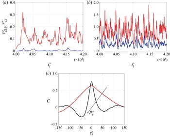
and the near-wall turbulence production are further examined. Figure 16 shows the time evolution of $\mathcal {P}_{\varOmega,l}^{+}$ and $T_{v,l}^{+}$ and their temporal cross-correlations for ZPG and for strong APG. For ZPG, the magnitude of $\mathcal {P}_{\varOmega,l}^{+}$ is much greater than that of $T_{v,l}^{+}$, although the peaks of $\mathcal {P}_{\varOmega,l}^{+}$ and $T_{v,l}^{+}$ often appear together (figure 16a). We note that the significant difference in the magnitudes of $\mathcal {P}_{\varOmega,l}^{+}$ and $T_{v,l}^{+}$ presumably reflects the existence of the other turbulence production mechanism for ZPG (i.e. the self-sustaining process). However, the cross-correlation between $\mathcal {P}_{\varOmega,l}^{+}$ and $T_{v,l}^{+}$ in this case (red line in figure 16c) is still non-negligibly large, indicating that the proposed production mechanism involving the Orr mechanism is also active even at ZPG. Indeed, a very recent study by Doohan et al. (Reference Doohan, Willis and Hwang2021) showed that such a mechanism exists in the near-wall region under ZPG, although the wall-normal transport of the wall-normal velocity fluctuation in their case was shown to originate from the energy cascade of larger structures (note that the simulation in this subsection is based on the minimal flow units for the near-wall region of the lower channel, which does not admit structures larger than the near-wall ones). For strong APG, the values of $\mathcal {P}_{\varOmega,l}^{+}$ and $T_{v,l}^{+}$ emerge at the same order and they seem to show much stronger correlation (figure 16b and black line in figure 16c), indicating that the proposed turbulence production mechanism is highly active, presumably due to the absence of the self-sustaining process.

Figure 16.

Temporal evolution of $\mathcal {P}_{\varOmega,l}^{+}$ (red lines) and $T_{v,l}^{+}$ (blue lines) with (a) $P_{x}^{+}=0.0$, (b) $P_{x}^{+}=0.012$. In (c) the temporal cross-correlation function of $\mathcal {P}_{\varOmega,l}^{+}l$ and $T_{v,l}^{+}$ is given for $P_{x}^{+}=0.0$ (red), $P_{x}^{+}=0.012$ (black).

The relevance of the proposed mechanism is also examined in a large computational domain to show that it is not an artefact taking place only in the minimal flow units. Figure 17 shows the instantaneous spatial distribution of integrands for $T_{v,l}^{+}$ and $\mathcal {P}_{\varOmega,l}^{+}$ in the near-wall region of the lower channel under strong APG. The instantaneous fields of the integrands for $T_{v,l}^{+}$ and $\mathcal {P}_{\varOmega,l}^{+}$ are highly localised in space, but most of them are found to be collocated in space. As mentioned earlier, any turbulence production mechanism in shear flows should involve an amplification process of fluctuations supported by the linearised Navier–Stokes equations (Cho et al. Reference Cho, Hwang and Choi2018). In the absence of any linear instability mechanism in the mean flow like the present case, only two linear mechanisms (i.e. the lift-up and Orr mechanisms) and their combination are viable for turbulence production (Farrell & Ioannou Reference Farrell and Ioannou1993; Jiao et al. Reference Jiao, Hwang and Chernyshenko2021). In particular, the Orr mechanism has been shown to be highly active for the structures with relatively short streamwise length scale (Jiao et al. Reference Jiao, Hwang and Chernyshenko2021). Therefore, the highly localised nature of the integrands for $T_{v,l}^{+}$ and $\mathcal {P}_{\varOmega,l}^{+}$ in space (figure 17) supports the relevance of the Orr mechanism initiated by the wall-normal nonlinear transport under strong APG.

Figure 17.

Isosurface of turbulent production $\mathcal {P}^{+}_{l}=7$ (red) and wall-normal turbulent transport $T_{v,l}^{+}=15$ (blue) at (a,b) two different time instants for $P_{x}^{+}=0.009$.

Finally, it should be mentioned that the Orr mechanism is a transient amplification process which requires an external driving mechanism for its activation. Therefore, the strong correlation between the nonlinear wall-normal transport of wall-normal velocity and the near-wall turbulence production implies the following causality relation: (1) a blob of wall-normal velocity fluctuation created from turbulence dynamics above the near-wall region is transported towards the near-wall region; (2) the Orr mechanism, which cannot be triggered in the absence of any initial wall-normal velocity fluctuation (see discussion above (Orr Reference Orr1907; Farrell & Ioannou Reference Farrell and Ioannou1993; Jiménez Reference Jiménez2013; Jiao et al. Reference Jiao, Hwang and Chernyshenko2021)), is subsequently activated by the blob of the wall-normal velocity fluctuation with an increased turbulence production. From this causality relation, the nature of outer turbulence now becomes important. In the minimal flow unit, the nonlinear wall-normal transport would stem from the self-sustaining process near the top wall or that in the middle of the channel (Yang, Willis & Hwang Reference Yang, Willis and Hwang2018), whereas, in the large computational domain, it may well be possible from the large-scale coherent structures in the middle of the channel and their energy cascade. This observation suggests the importance of outer turbulence in the near-wall dynamics in the presence of APG, and this is particularly true when the intrinsic self-sustaining mechanism of near-wall turbulence is destroyed. However, the mechanism we proposed here for the near-wall region is generic in the sense that the nonlinear wall-normal transport and the Orr mechanism are mathematically well-defined processes in terms of the Navier–Stokes equations. This is why we observed the same processes in the minimal flow unit and in the large computational domain, although the nature of outer turbulence in the two different computational domains is different. In this respect, it would be interesting to examine the existence of the observed mechanism in more complex flows in the future.