


I. Introduction
The following attempt to formulate approximately the equilibrium configuration and particularly the equation for the firn surface of an ice sheet in steady state has been inspired primarily by the following researches: experimental and theoretical studies of English and Swiss physicists and glaciologists,Reference Glen 1 , Reference Nye 2 , Reference Robin 3 , Reference Haefeli and Kasser 4 , Reference Steinmann 5 results of the Expéditions Polaires Françaises of P. E. Victor,Reference Holtzscherer and Bauer 6 and investigations carried out during 1950–60 in the cold ice cap of the Jungfraujoch.Reference Haefeli and Brentani 7
We shall treat first of all the main problem, that of the plane, steady-state motion and form of the surface profile in the firn region of a long, strip-shaped ice sheet (Fig. 1a) under constant accumulation. The desired function is of the form

where
-
y = ice thickness at a point P on the firn surface, a distance x from the center A of the ice sheet (Fig. 1a) .
-
H = maximum ice thickness in the ice sheet, at point A.
-
a = yearly accumulation (thickness of the layer of ice, of assumed density ρ = 917 kg./m.3 formed each year).
-
k, n = ice flow law parameters (see equation 2) .
Strip-shaped and circular ice sheets. (a) Strip-shaped ice sheet, (b) Circular ice sheet. a = accumulation per year

After the general equation (1) of the firn surface has been derived from the condition of continuity and the flow law of Glen,Reference Glen 1 it is possible to compare the theoretically calculated surface profile AC (Fig. 1a) with that measured by the Expéditions Polaires Françaises (Fig. 6). The comparison is made by constraining the theoretical curve to pass through two given points, the summit point A and an arbitrary second point C (with coordinates c, h) lying above the firn line, and then choosing the flow-law parameters k and n so that, for the known accumulation a, the best agreement between calculated and measured surface profiles is obtained.
Next the equation for the surface profile of a circular ice sheet (Fig. 1b) is formulated, the differential equation for which differs only by a form factor from that of the strip-shaped ice sheet. In addition, certain general relations between the accumulation a and the maximum ice thickness H are established and illustrated by examples.
II. Experimental and Theoretical Basis
We use as the most important experimental basis for the following treatment the flow law of Glen,Reference Glen 1 which has been confirmed by numerous recent investigations and may be considered a good approximation for polycrystalline glacier ice. It reads (see Fig. 2)

where z is the coordinate in the vertical direction and τ is the shear tress across the horizontal plane. The parameter k depends principally upon the temperature of the ice,Reference Glen 8 whereas the exponent n depends among other things on the crystallographic relationships and the strain-history of the ice type concerned.Reference Steinmann 5 In order that the temperature-dependent parameter may have easily understood dimensions, we write equation (2) in the following form:

in which τ 1 is the unit of shear stress. For τ = τ 1, we have ϵ = k 1, from which the parameter k 1, can be defined as that rate of deformation (rate of simple shear in sec.−1 or yr.−1) which takes place under the unit of stress τ 1. The lower the temperature, the smaller is the value of k or k 1. The relation between parameters k and k 1, which differ only in units, is:

Flow curve of polycrystalline ice. μ = “apparent viscosity”

In order to express the flow curve of ice as that of an incompletely viscous fluid, and to facilitate comparison with a Newtonian-viscous fluid, it is useful to introduce the “apparent viscosity” μ, which, on the basis of equations (2)–(4) and Figure 2, is defined as follows:

For τ = τ 1;

For τ = τ 2;


For the special case n=1, the apparent viscosity, which is defined as the tangent of the angle μ* which a radius vector to the flow curve makes with the axis of ordinates (Fig. 2) becomes identical with the Newtonian viscosity η, that is

Since the temperature in the ice sheet varies from place to place, we must, strictly speaking, deal with a spatially varying k 1, value. The fact that both the ice temperature and the shear stress in general increase downward along a vertical profile through the ice sheet and reach their maximum values at the bed produces a very strong curvature in the lower part of a vertical profile of the horizontal velocity component, shown in Figure 3, as Nye has already pointed out.9 If for simplicity a constant, average k value is assumed, then the resulting error can be partially compensated by a relatively high n value, as is shown later. (The velocity profile shown in Figure 3 corresponds, for example, to the n = 4 for constant k.)
Vertical velocity profile (horizontal component)

It should be noted furthermore that, because of the lower viscosity of the surficial firn layers, the velocity profile displays a small anomaly in the form of a local, surficial peak, as has been often observed in the snow cover and in alpine firn regionsReference Hacfeli 10 and is presently under investigation on the Greenland Ice Sheet by the International Greenland Glaciological Expedition.Reference Haefeli 21 Thanks to the relatively small thickness of the firn layer in relation to the total ice thickness, this anomaly will be taken into consideration in the balance condition (continuity) only insofar as, in calculating the ice flux from the velocity profile, the velocity at the surface is taken to be not the actual value υ x max but instead the theoretical value that would be present if the firn cover were replaced with ice. The value υ xm given in Figure 3 indicates accordingly the average horizontal velocity component outlined by arrows, according to the equation

III. Assumptions
The theory developed is based on the following assumptions:
-
The flow law of Glen (equation 2) is independent of the magnitude of the superimposed hydrostatic pressure, as has been demonstrated experimentally for single crystals up to pressures of 350 kg. cm.−2 by Rigsby.Reference Rigsby 12
-
The flow is laminar and steady, and takes place so slowly under the influence of gravity and internal friction that the forces due to acceleration are negligible.
-
Within the firn region CAC in which the equation of the surface profile is calculated, the accumulation a is assumed to be constant (Fig. 4)
-
Within the entire firn region FAF the ice is assumed not to slide on its bed (v u = 0). It is immaterial whether this condition is the result of the ice being solidly frozen to the glacier bed (permafrost), or of a great roughness of the contact surface, or of relatively small shear stresses, or whether the combined action of two or more of these factors is responsible. It is nevertheless probable, on the basis of investigations by Robin,Reference Robin 3 Holtzscherer,Reference Holtzscherer and Bauer 6 and the author,Reference Haefeli and Brentani 7 that in the centre of the Greenland Ice Sheet the ice is frozen solidly to the bed and rests on a permafrost lens of unknown thickness and extent.
-
The bed of the ice sheet is assumed horizontal. In the case of an irregular bed having variations in elevation of ±10 per cent of the total ice thickness (as in Greenland), the substitution of a horizontal plane at the same average elevation as the actual, irregular bed gives a useable approximation (cf. Fig. 6). Extension of the theory to an inclined bed poses no particular difficulties.
-
The actual parameter k, which in fact varies with temperature and hence from place to place,Reference Glen 8 , Reference Steinmann 13 is for simplicity replaced with a constant “standard average value” k. In order to obtain, in spite of this, a good agreement between measured and calculated surface profiles, a fictitious value of n must be chosen that is somewhat larger than the experimentally determined values.Reference Butkovich and Landauer 22 By this artifice the error made by assuming a constant value of k is, as already mentioned, partially compensated.
-
The treatment deals only with the horizontal component of velocity, which alone enters into the consideration of balance (continuity). The validity of the treatment is restricted to the firn region. It gives a useful approximation, but not an exact solution.
Cross-section through an ice sheet with streamlines (schematic). a = accumulation in m. of ice per year, c = half-width offern region with average accumulation a, f = half-width offern region, F = firn line, b = semi-major axis of ellipse 1, S = crevasse zone, 1 = firn surface, 2 = streamlines, 3 = velocity profile, 4 = ice temperature in the centre, 5 = isotherm, 6 = permafrost, 7 = pressure melting point
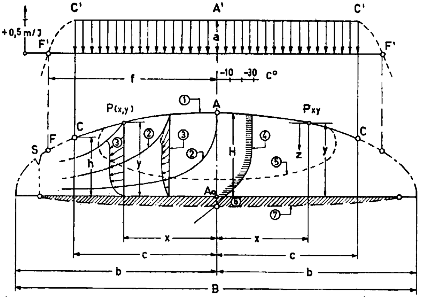
Equilibrium state of strip-shaped we sheet (approximate solution). H = maximum thickness of ice = semi-minor axis, a = accumulation (in m. of we per year), b = semi-major axis of curve ACT, ρ = density of ice (917 kg./m.3), F = fire line

East-west profile through the Greenland Ice Sheet, comparison of theoretical and measured profiles. 1 = firn surface for n = 1, 2 = firnsurfacefor n = 2, 3 = measured firn surface (E.P.F.), 4 = firn surface for n = 4, 5 = average horizontal velocity of a vertical profile, 6 = slope of firn surface in per cent (n = 4), 7 = shear stress on bedrock (kg./cm.2) for n = 4, 8 = velocity profile of a vertical section (horizontal component, m./yr., n = 4), 9 = distribution of shear stress in a vertical section (kg./cm.2, n = 4), 10 = constant accumulation (A−C) a = 0.5 m./yr., 11 = variation of accumulation after Diamond in m. of water per year, 12 = theoretical bed, 13 = bed as determined by seismic sounding (Holtzscherer, E. P. F.), 14 = bed as determined by gravity measurements (Holtzscherer, E. P. F.)

IV. Basic Equations for a Strip-Shaped Ice Sheet
1. General considerations
From the foregoing explanation (I–III) and the situation depicted in Figure 5, the following basic relations emerge:
Slope of the firn surface:

Shear stress across horizontal and vertical planes τxz = τ:

From equations (2) and (3):

Mean horizontal velocity:

Equation (10) is the continuity condition that applies to the steady state of the ice sheet.
2. Velocity distribution along a vertical line (vertical velocity-profile)
From equations (8) and (9) it follows (see Fig. 5) that


The average horizontal velocity vxm is thus obtained as :


3. Differential equation of the firn surface
From equations (7), (10) and (13) the following differential equation for the surface profile is obtained:

4. Equation of the curve AC of the surface profile
From equation (14) it follows that:

The integration of this differential equation results in the following expression for the ice thickness y as a function of distance x from the centre of the ice sheet:

For x = 0, y = H; hence C 4 = nH 2(n+1)/n /2(n+1) ,

As equation (15) shows, we deal here with a closed curve of elliptical character, with semi-minor axis H and semi-major axis b, which is given, on setting y = 0 in (15), by:

It is to be noted that the portion of the curve CFT has only mathematical, not real, significance. For this reason b does not need to agree with the half-width of the ice-sheet. Note further that the curve for y has a horizontal tangent at A and a vertical tangent at T. The former is real, because the firn surface has a maximum at the summit point A.
5. Determination of parameters n and k
If for a given ice sheet there are given, beside the summit point A, the coordinates (x, y) of two additional surface points, then from equation (15) the average values k and n appropriate to the case concerned can be calculated.
If at first n is left unspecified and k is calculated as a function of n by taking as given only one marginal point C, with coordinates (c, h), in addition to the centre point A, then from equation (15) the following value for k is obtained:

n can now be varied until the measured surface profile agrees as nearly as possible with the profile calculated from equation (15) for a given a.
On the other hand it is also possible to eliminate the parameter k by introducing its value from equation (17) into equation (15). The following expressions are thereby obtained:


For

Note that in this case y (equation (19)) and b (equation (20)) depend, for given coordinates of the points A and C, only on the parameter n.
V. Application to the Greenland Ice Sheet
Figure 6 shows the transverse profile measured by the Expéditions Polaires FrançaisesReference Holtzscherer and Bauer 6 , Reference Tschaen 29 and re-measured in 1959 by the International Greenland Glaciological Expedition. In accordance with section IV, 5 we proceed as follows in comparing the measured and calculated profiles:
From the measured profile (Fig. 6), we choose, beside the summit point A with H = 3,160 m. the point C, above the firn line, at an elevation of 2,000 m. as the end-point of the function y. The distance between points A and C is c = 385 km.
The average annual accumulation between points A and C is estimated, according to DiamondReference Diamond 14 (see Fig. 6, curve 11), as 45 cm. of water or 50 cm. of ice (a = 0·50 m. yr.−1) ; the actual accumulation is larger in the western part than in the eastern. Based on firn stratigraphy, Sorge determined a mean annual accumulation of 31.4 cm. of waterReference Sorge and Brockamp 15 , Reference Bader 16 at station “Eismitte.”
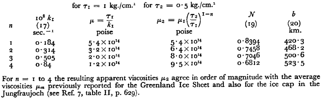
In Table I are given values of the various subsidiary quantities k 1, μ 1, μ 2, N and b calculated from equations (5), (17), (19) and (20) for a = 0·50 m./yr., and for integral values of n from 1 to 4.
Subsidiary Values k 1, μ 1, μ 2, N and b for various n
The calculation represented in Figure 6 shows that the difference between the surface profile calculated for n = 4 and that measured by E.P.F. amounts to less than 1 per cent of the ice thickness. The analytically derived points lie on the whole only about 0.5 per cent lower than the measured pointsReference Holtzscherer and Bauer 6 whereas the curve calculated for n = 2 lies considerably above the measured points. The best agreement between measurementReference Holtzscherer and Bauer 6 and calculation would be obtained for an n-value between 3 and 4, and in fact nearer to 4.Footnote *
Note that the profile calculated for n = 4 (Fig. 6) agrees relatively well with the measured profile even below the point C, where strictly speaking it no longer has real significance. Also noteworthy is the relatively large discrepancy between the measured profile and the solution for a Newtonian fluid (curve 1, for n = 1).
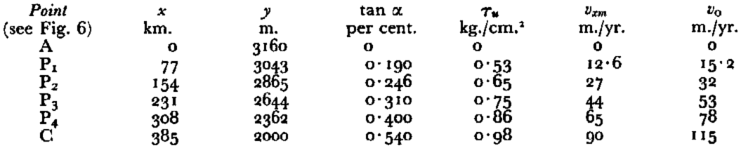
Values for the surface slopes (Fig. 6, curve 6), the shear stresses τu at the bed (curve 7), and the mean velocities vxm across vertical sections (curve 5) are given in Table II.
Calculated Values of tanα, τ u , v xm AND v 0 (n = 4)
VI. Basic Equations for a Circular Ice Sheet
Derivation of the surface-profile equation for a circular ice sheet follows the same lines as that for a strip-shaped sheet; the only difference is in the balance or continuity equation, which here reads (where x = radius vector) :

(instead of ax/y as in equation (10)). The corresponding basic equations are:


(See Fig. 11, p. 1151.)



VII. Some Special Applications
The following four examples are selected from among the various possible applications of the theory developed above.
1. Calculation of the average accumulation of an ice sheet in a steady state
If the approximate form of the surface profile is known (H, h and c) and also the values k and n, then from equation (17) or (17a) the quantity a can be calculated. For the circular ice sheet, for example, we find from equation (17a):

As a numerical example we choose an ice sheet of dimensions similar to the Antarctic Ice Sheet and assume the values k and n (in particular n = 3) given by analysis of the Greenland Ice Sheet (profile E.P.F.). If the firn line lies near sea-level, h can be neglected in comparison with H, so that equation (21) simplifies to:
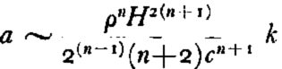
Assuming ρ = 900 kg.m.−3, H = 4,500 m., c = 2,000 km., τ 1=1 kg.m.−2, n = 3 and k = k1 = 0.505 × 10⁻²⁰ sec.−1 (Tables I and II) we find:

The question remains open, whether by this indirect approach a contribution can be made to solution of the problem of accumulation in the Antarctic. Clearly the application to Antarctica of results obtained in the Arctic and in particular in the Greenland Ice Sheet can be made only with the greatest caution and with recognition of the distinctly different conditions. Within the scope of the present study, all that can be done is to point to certain general relationships between the balance condition on one hand and the rheological requirements on the other.Reference Vyalov 17 , Reference Mellor 18 , Reference Loewe and van Rooy 19 , Reference Lister and Pratt 20
2. Relations between accumulation and maximum thickness of an ice sheet in a steady state
(a) For fixed values of ρ, n and k, it follows from equation (22) for (h = 0) that:
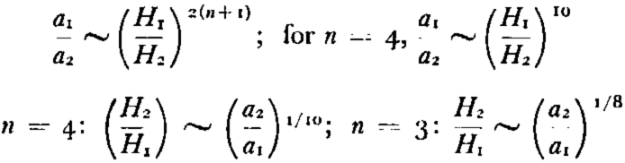
It follows from this that the ice thickness H is very insensitive to change in accumulation, and the more so, the higher the value of n. If for example a 2 = 2a, that is, were the accumulation doubled without changing k, an increase in ice thickness of only 7.8 per cent for n = 4 or about 9 per cent for n = 3 would suffice to restore a stationary state. For n = 1, that is, for a Newtonian-viscous fluid, the corresponding percentage increase would however amount to 19, so that the ice thickness would react rather more sensitively to changes in a. For a 10-fold increase in accumulation (e.g. from 5 cm. to 50 cm. ice per year) over an ice sheet of approximately the dimensions of Antarctica, the percentage increase in ice thickness would for n = 4 (and the corresponding k value) amount only to 26 per cent, or for n = 3 to 33 per cent.
(b) The ice sheet under consideration would react somewhat more sensitively if, instead of a change in precipitation, a change in the temperature of the deep-seated ice were to take place, due, for example, to a change in the geothermal heat flux. The relation pertinent to such a change reads, for our special case (h = 0),
(23)

The closer the temperature approaches the pressure melting point in the basal ice, the greater k becomes there, and in fact a temperature increase of 1° C. is sufficient to cause a many-fold increase in k. Under the assumption for example that the pertinent k value were to increase ten-fold, the ice thickness H would, according to equation (23), decrease by about 20 per cent, in order to restore a stationary state. Thus in this case, too, a relatively insensitive response of the ice sheet is found. This is especially true also for variations in the average air temperature, as long as this temperature remains below the freezing point.
On the other hand it should be remembered in this connection that the stationary state, which is all that has been considered up to now, is in fact a rare exception that, strictly speaking, is reached and quickly passed through only during the transition from positive to negative mass budget or vice-versa. If a stationary state has been attained under long-constant climatic conditions, and if the climate then suddenly changes, the new conditions remaining thereafter again constant, it may well take thousands of years for the ice sheet to reach the steady state adjusted to the new climatic conditions.
In relation to non-stationary states, furthermore, the problem of stability must be considered. For the central part of the ice sheet, the conditions for stable response are well satisfied, because it is a region of extending flow.Reference Nye 24 In the marginal zone the behaviour of ice sheets is very sensitive to any change of sliding conditions on the glacier bed.
From the viewpoint of ice-cap rheology as developed in the present paper, it seems hard to assess the age of the upper edge of the 200 to 300 m.-high bright band of less-weathered rock observed above both sides of the Jakobshavns Isbrae, and above other great ice streams in Greenland. A future dating of this level would be of great help in the study of the behaviour of ice sheets.Reference Georgi 31 , Reference Weidick 34
3. Age of the ice in the Greenland Ice Sheet
A final application of the present theory, closely related to the phenomena just discussed, is the calculation of the age of the ice in various parts of the ice sheet, and the calculation of “travel times” for the ice-particle trajectories. Specifically, how long does it take for an ice particle or any other object, deposited on the surface in the central part of the Greenland Ice Sheet at a distance x from the middle point A, to reach the coast?
This question can be answered to a first approximation, good for a large part of the firn region, by calculating the “travel times” simply from the average horizontal velocity component v xm for each vertical profile (equation (10)). The resulting travel times for trajectories originating in the outer two thirds of the fern surface are somewhat (c. 5 to 20 per cent) too Iarge, because for these trajectories the actual horizontal velocity components v x are somewhat Iarger than the average velocity v xm (see Fig. 7). On the other hand, for trajectories originating in the central part of the firn surface and therefore descending so deeply into the ice sheet that they approach the bottom, where due to the boundary conditions the velocity approaches zero, the true velocity components v x are considerably smaller than the averages v xm and the corresponding travel times thus considerably greater than given by the simplified calculation based on the average velocity. The result of the approximate calculation is shown in Figure 7, in which the total travel time, from starting point x to the glacier edge, is plotted as a function of x. In the calculation of total travel time, which is only of relative significance the assumption is made that a rectangular accumulation area of 450 km. length and 175 km. width (half-width of the area studied by the International Greenland Expedition 1957–60) feeds at its coastal edge into a single great ice stream, 70 km. long, in which the average forward velocity (including basal slip) accelerates from 150 m.yr.−1 at its head to c. 7,000 to 8,000 m.yr.−1 at its snout. Such a glacier would exceed the Jakobshavns Isbrae in its production of icebergs.Reference Georgi 31
Mean velocity vx and total travel time T as a function of x (distance from centre A). 1 = for rectangular drainage area, 2 = for triangular drainage area, on east-west profile through the Greenland Ice Sheet
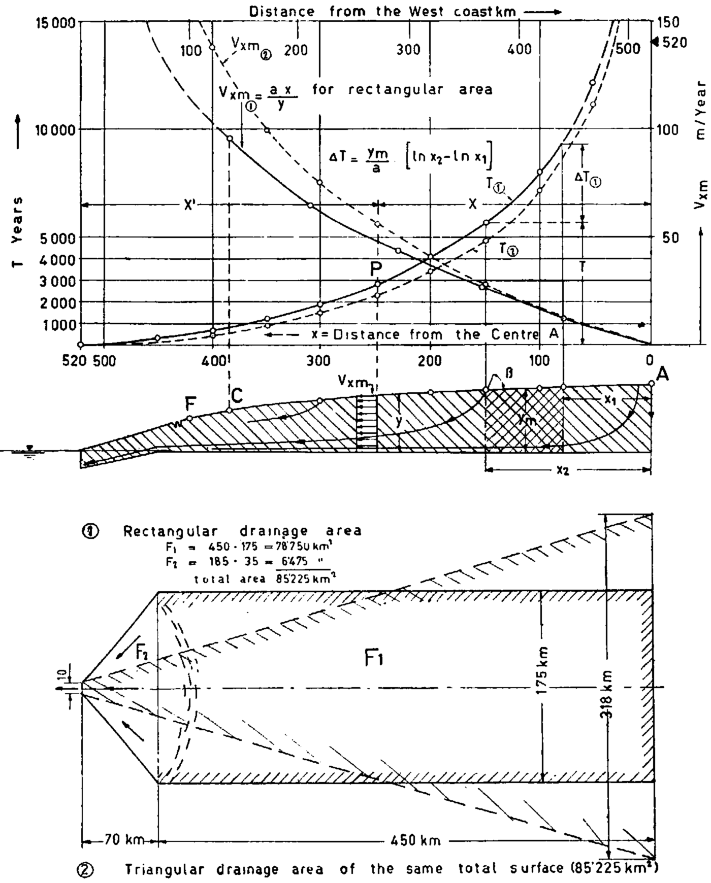
The approximate travel-time calculation can be made from the average ice velocity (obtained from the continuity condition and the ice thickness) by dividing the entire path into a sufficiently Iarge number of small segments.Reference Haefeli 26 The time ΔT required to traverse a segment of length Δl=x 2−x 1, is thus calculated as:

where y m is the mean ice thickness of the segment (treated as constant over the length of the segment). It must be remembered that, as already mentioned, this approximate calculation becomes invalid for the deepest trajectories, yielding travel times much too small. For these trajectories only a determination of the exact shape of the trajectories and a calculation of the velocity distribution along them would lead to the theoretically correct result. The trajectories having travel times of 10,000, 20,000, 30,000 years and more could thus be found, and from them an overall idea of the rheologically possible age distribution of ice in the ice sheet could be obtained, the entire ice sheet being subdivisible into zones of successively greater age.
On the other hand the age and origin of the ice can nowadays be determined approximately by the purely experimental methods of nuclear physics. The results obtained in this way from a Danish expedition agree at least in order of magnitude with the values calculated theoretically above.Reference Dansgaard 27 In this respect, one need not be surprised that with the usual method of ice sampling from icebergs, it has not hitherto proved possible to collect and study very old ice, from the central zone near the summit point of the ice sheet, which can only be found near the glacier bed and thus only in very particular places on freshly calved specimens of the biggest icebergs from the biggest ice streams. Moreover, the very oldest ice, in the immediate neighbourhood of the glacier bed, cannot reach the ocean at all, because in the ablation zone a certain thickness of ice must be melted away from the glacier bottom, on account of the geothermal heat flux and of frictional heating.
The determination of ice travel times has recently become a timely matter, in relation to the proposal by the German physicist Bernhard Philberth to solve the difficult problem of disposal of radioactive wastes from nuclear reactors by using the great ice sheets of the earth as burial grounds.Reference Philberth 28 By investigations in glaciology and nuclear physics it has been shown that the “partial travel times” of radioactive wastes deposited in suitable form in the summit of the great ice sheets are several times larger than the period of c. 1,500 years necessary for decay of the dangerous radiation. The designation “partial travel time” is used here for the time necessary to traverse the firn region, which is the time elapsed before the radioactive wastes come into contact with circulating water. Because the basic requirement for disposal of radioactive wastes would thus be fulfilled to a degree not attained by any other known procedure, Philberth’s proposal deserves serious consideration in spite of the extraordinarily difficult problem of transportation, and all the more so now that oceanographers have expressed the most serious reservations for the future mankind if highly radioactive waste is deposited in the oceans.
VIII. Additional and Concluding Remarks
The theory here presented of the overall relief and velocity distribution in the firn region of an ice sheet was developed primarily as a working hypothesis for the rheological programme of the International Greenland Glaciological Expedition in 1959.Reference Haefeli 21 It also served in part to determine the accuracy of measurement required in the geodetic work. Final judgement on the applicability of these theoretical considerations will only be possible on the basis of the results of the expedition when they have been finally evaluated,Footnote * these at present are still being studied, with the results of further expeditions to the Arctic and Antarctic.
The present study was carried out roughly simultaneously with a very important investigation by J. F. Nye which treats a similar subject.Reference Nye 32 In spite of the fact that the two independent investigations proceed from different assumptions, they arrive at similar conclusions regarding the striking insensitivity of the total ice thickness H of the ice sheet to changes in accumulation.
The connection between the present theory and the theory developed by Nye for the “form and motion of ice sheets” stems from the following mathematical relations:
(a) Motion of the ice sheet
This is characterized among other things by the form of the velocity profile, which for any vertical cross-section (at x) can be expressed by the ratio of the velocity component v xm at any given depth z to the average cross-section velocity v xm (see equations (11) and (12)):


For

From this it is seen that the rectangular velocity profile of Nye corresponds to the special case of n=∞ (cf. Fig. 8). But Nye’s results will agree much more closely with ours than this suggests, because in his case the ice motion is governed by sliding at or near the bed in response to a power-law flow relation with a high value of n.
Velocity profile through an ice sheet for various values of the power-law exponent n

(b) Form of the ice sheet
For the special case h = 0 (constant accumulation over the entire surface of the ice sheet, or firn line at the elevation of the horizontal bed of the ice sheet, that is, at sea-level) we have from equation (19) for the strip-shaped ice sheet:

where y =y/H and x =x/b
For the circular ice sheet there follows in the same way, from equation (19a):

where y =y/H and x =x/r.
These two equations show that the relative shape of an ice sheet is independent of the accumulation a and the parameter k and depends only on n. For r = b the two equations become identical, so that the saine shape-relation holds for the circular and the strip-shaped ice sheet. In Figure 9 this shape relation is shown for various values of n. For n=∞ there results the parabola of Nye,Reference Nye 2 which is also obtained in Nye’s more recent formulation Reference Nye 32 by putting m=∞. Finally in Figure 10 is shown a comparison between the theoretical surface profiles for n=1, 3, 4, ∞ and two measured profiles of the Antarctic Ice Sheet, taken from the map prepared in October 1958 by the American Geographical Society for the National Academy of Sciences. From this comparison the following points emerge. The profile
Surface profile of an ice sheet for various values of the power-law exponent n

Profiles through the Antarctic Ice Sheet, comparison of theoretical and measured profiles

“An ice cap as the throne of the Gods.” Shining (6,542 m.), Garwal, Himalaya. A graphic demonstration of the fact that, according to equation (16a), H/r gets larger when r gets smaller!

A1—B2 measured by the Commonwealth Trans-Antarctic Expedition between the Filchner Ice Shelf and the summit point of the ice sheet lies between the theoretical profile for n = 4 and n = ∞ . The relatively great undulations in the detailed topography of the ice surface point to large topographic irregularities in the bed of the ice sheet, with local depressions. On the basis of the profile A1−B at long. 90° between the summit (4,000 m.) and the Davis Sea it seems at first sight necessary to postulate the existence at the margin of the continent of a subglacial mountain range, over which the ice sheet flows as over an ice fall. On the other hand we should not forget that our assumption of a constant accumulation within the firn region is very far from being fulfilled in reality. The relatively high marginal accumulation observed by different explorers can have a similar effect on the shape of the profile as a discontinuity in the bed. If for example all accumulation were concentrated in a ring-shaped zone at the margin of a circular ice sheet, it is evident that the central zone of no accumulation would be horizontal, bordered by a relatively steep marginal zone.
The author is especially indebted to Prof. B. Kamb for his careful English translation of this paper and to Dr. J. W. Glen for his valuable comments made in Helsinki 1960. He is also indebted to the Schweizer Nationalfond zur Förderung von wissenschaftlichen Forschungen, which enabled him to take part in the International Greenland Glaciological Expedition, 1957–60.



