1 Introduction
Helical vortices are elementary flow structures that have received much attention over the years. This interest is partly due to their appearance in applications related to industrial flows involving, for instance, horizontal-axis wind turbines (Vermeer, Sørensen & Crespo Reference Vermeer, Sørensen and Crespo2003), marine propellers (Felli, Camussi & Di Felice Reference Felli, Camussi and Di Felice2011), swirling jets (Meliga, Gallaire & Chomaz Reference Meliga, Gallaire and Chomaz2012) and helicopters (Leishman Reference Leishman2006).
Central to the study of vortex dynamics is the question of instability, which is found to have direct consequences for some of the applications mentioned above. Examples include wind farms, where an unperturbed wake consisting of coherent helical tip vortices imposes a much higher loading on a downstream turbine than a turbulent wake (Sørensen Reference Sørensen2011), and rapidly descending helicopters, where an instability of the helical tip vortices may be related to the onset of the dangerous vortex-ring state, characterised by strong thrust fluctuations and a sudden loss of lift (Leishman, Bhagwat & Ananthan Reference Leishman, Bhagwat and Ananthan2004).
The interaction between concentrated vortices can lead to different types of instabilities. They can be divided into displacement instabilities, where the vortex core is locally shifted as a whole, and core instabilities, which modify the internal structure of the core, as discussed by Leweke, Le Dizès & Williamson (Reference Leweke, Le Dizès and Williamson2016) for vortex pairs and Leweke et al. (Reference Leweke, Quaranta, Bolnot, Blanco-Rodríguez and Le Dizès2014) for helical vortices. The present work is concerned with the former type. The first comprehensive account of the stability of a single helical vortex filament with respect to infinitesimal displacement perturbations was given by Widnall (Reference Widnall1972), who determined their evolution and growth rates using the self-induced velocities from the Biot–Savart relation. Widnall (Reference Widnall1972) identified unstable modes at different wavelengths, characterised by out-of-phase perturbations on neighbouring loops of the helical vortex. Gupta & Loewy (Reference Gupta and Loewy1974) later extended this work to configurations with multiple interdigitated helices, calculating the growth rates of unstable modes using the self- and mutually induced velocities again through the Biot–Savart formalism.
A more recent study addressing the issue of stability in an array of helical vortices is the one by Okulov (Reference Okulov2004). Unlike earlier efforts relying on the integration of the Biot–Savart law, Okulov considered an expression of the induced velocity involving Kapteyn series, first established by Kawada (Reference Kawada1936) and later again by Hardin (Reference Hardin1982), and was able to provide an analytical solution to the problem. The results were used to predict the instability of helical vortex systems (e.g. in Okulov & Sørensen Reference Okulov and Sørensen2010) with respect to uniform deformations (contraction, dilatation) of each vortex.
Stability problems of this type are today routinely addressed using numerical simulations. Examples concerning helical vortices include the studies of Ivanell et al. (Reference Ivanell, Mikkelsen, Sørensen and Henningson2010) and Sarmast et al. (Reference Sarmast, Dadfar, Mikkelsen, Schlatter, Ivanell, Sørensen and Henningson2014), who modelled the wake of a rotor with the actuator line method (Sørensen & Shen Reference Sørensen and Shen2002). These authors performed a spectral analysis of the resulting nonlinear flow and determined the spatial growth rates of the individual modes. The temporal linear stability problem was also recently revisited by Selçuk, Delbende & Rossi (Reference Selçuk, Delbende and Rossi2018), who determined the growth rates and corresponding unstable modes of a helix configuration via time-stepping methods applied to the linearised Navier–Stokes equations.
Whereas the theoretical and numerical development has been thriving in this field, precise experimental studies concerning the dynamics and instabilities of helical vortices are rather scarce. Although the existence of an instability involving vortex pairing had been observed already by Alfredsson & Dahlberg (Reference Alfredsson and Dahlberg1979), quantitative comparisons between experiment and theory have largely remained absent. One attempt is the study by Nemes et al. (Reference Nemes, Lo Jacono, Blackburn and Sheridan2015), who considered the wake of a two-bladed rotor and presented a comparison between the experimentally estimated growth rates and those reported by Widnall (Reference Widnall1972) and Gupta & Loewy (Reference Gupta and Loewy1974). However, due to the lack of a controlled method for perturbing the vortices, the data exhibited a large amount of scatter that prevented the identification of individual modes. In the recent study reported in Quaranta, Bolnot & Leweke (Reference Quaranta, Bolnot and Leweke2015), a series of experiments on a single helix generated by a one-bladed rotor were performed. Different instability modes could be individually excited through controlled perturbations, and very close agreement between the theoretical and experimental mode shapes and growth rates was found.
In the present study, the work of Quaranta et al. (Reference Quaranta, Bolnot and Leweke2015) is extended to the configuration with two interlaced helical vortices. The article is structured as follows. In § 2, key results from previous theoretical work are recalled and applied to the two-helix configuration, and an analogy with the three-dimensional pairing instability of straight vortices is established. Then § 3 gives a description of the experimental set-up and the perturbation methods used to excite the instabilities. The presentation of the experimental results is divided into three parts. In § 4, the measured properties of the unperturbed rotor wake are presented; in § 5, the observations and measurements concerning the linear displacement instability are shown and compared to theoretical predictions; and § 6 covers the later stages of the instability, which is dominated by the nonlinear evolution of the perturbations. A summary of the main findings and conclusions are given in § 7.
2 Theoretical background
2.1 Base flow
A simplified model of a two-bladed rotor wake is given by a system of two infinite helical vortex filaments in a cylindrical coordinate system (
 $r,\unicode[STIX]{x1D703},z$
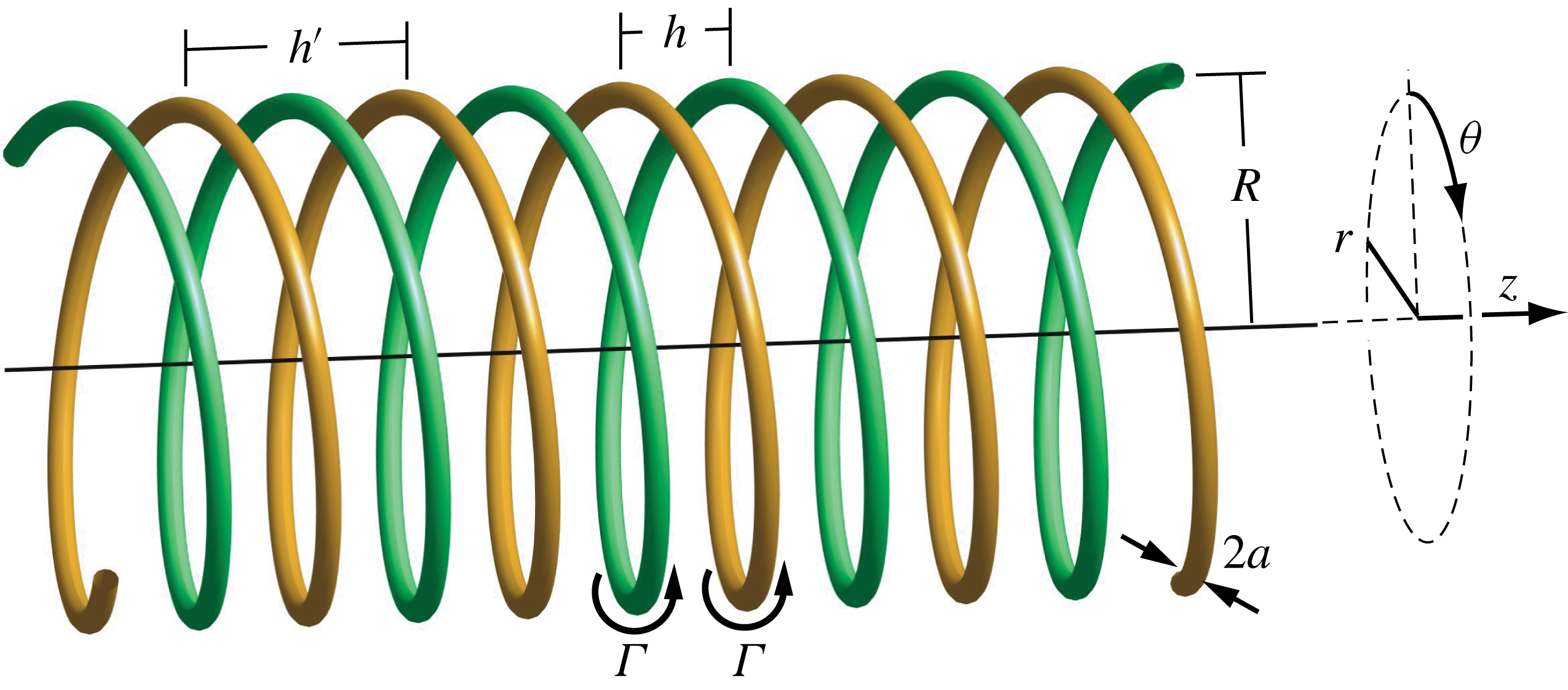
), as shown in figure 1. The defining parameters of the helix geometry are the radius
 $R$
and the pitch
 $h^{\prime }$
of the helical centreline of each vortex. The two vortices are separated azimuthally by an angle
 $\unicode[STIX]{x03C0}$
, and their unperturbed positions can be written as
 $$\begin{eqnarray}\boldsymbol{r}_{m}=\left(\begin{array}{@{}c@{}}r_{m}\\ \unicode[STIX]{x1D703}_{m}\\ z_{m}\end{array}\right)=\left(\begin{array}{@{}c@{}}R\\ \unicode[STIX]{x1D703}+m\unicode[STIX]{x03C0}\\ h^{\prime }\unicode[STIX]{x1D703}/(2\unicode[STIX]{x03C0})\end{array}\right),\quad \unicode[STIX]{x1D703}\in \mathbb{R},\end{eqnarray}$$
where
 $m=1,2$
is the helix index. The distance
 $h=h^{\prime }/2$
is the separation between neighbouring vortex loops at constant
 $\unicode[STIX]{x1D703}$
.
Schematic of two interlaced infinite helical vortices, including the relevant parameters: pitch
 $h^{\prime }$
of one helix, separation
 $h$
of neighbouring helix loops, radius
 $R$
, core size
 $a$
and circulation
 $\unicode[STIX]{x1D6E4}$
.

For the present analysis, the internal structure of the vortices is assumed to be that of a Batchelor vortex, characterised by Gaussian distributions of axial vorticity and velocity. In local cylindrical coordinates (
 $\unicode[STIX]{x1D70C},\unicode[STIX]{x1D719},\unicode[STIX]{x1D709}$
) of the vortex, the radial profiles of azimuthal and axial velocities read
 $$\begin{eqnarray}v_{\unicode[STIX]{x1D719}}(\unicode[STIX]{x1D70C})=\frac{\unicode[STIX]{x1D6E4}}{2\unicode[STIX]{x03C0}\unicode[STIX]{x1D70C}}[1-\exp (-\unicode[STIX]{x1D70C}^{2}/a^{2})]\quad \text{and}\quad v_{\unicode[STIX]{x1D709}}(\unicode[STIX]{x1D70C})=V_{\unicode[STIX]{x1D709}}^{max}\exp (-\unicode[STIX]{x1D70C}^{2}/a^{2}),\end{eqnarray}$$
where
 $\unicode[STIX]{x1D6E4}$
is the vortex circulation,
 $a$
is the core radius and
 $V_{\unicode[STIX]{x1D709}}^{max}$
is the amplitude of the core velocity.
The non-dimensional parameters characterising the flow are the Reynolds number
 $Re=\unicode[STIX]{x1D6E4}/\unicode[STIX]{x1D708}$
(where
 $\unicode[STIX]{x1D708}$
is the kinematic viscosity), the scaled vortex separation
 $h/R$
and core radius
 $a/R$
, and the axial flow parameter
 $$\begin{eqnarray}W=2\unicode[STIX]{x03C0}aV_{\unicode[STIX]{x1D709}}^{max}/\unicode[STIX]{x1D6E4},\end{eqnarray}$$
which represents the ratio between the maximum axial and swirl velocities. As discussed in Quaranta et al. (Reference Quaranta, Bolnot and Leweke2015), the relevant time scale for the development of the long-wave instability studied here is given by
 $2h^{2}/\unicode[STIX]{x1D6E4}$
, which is used to non-dimensionalise time
 $t$
, as well as the instability growth rate
 $\unicode[STIX]{x1D70E}$
and frequency
 $\unicode[STIX]{x1D714}$
, according to
 $t^{\ast }=t\unicode[STIX]{x1D6E4}/(2h^{2})$
,
 $\unicode[STIX]{x1D70E}^{\ast }=2\unicode[STIX]{x1D70E}h^{2}/\unicode[STIX]{x1D6E4}$
and
 $\unicode[STIX]{x1D714}^{\ast }=2\unicode[STIX]{x1D714}h^{2}/\unicode[STIX]{x1D6E4}$
(non-dimensional quantities are denoted with an asterisk).
We here also make use of the concept of an equivalent Rankine-type core size. Widnall, Bliss & Zalay (Reference Widnall, Bliss, Zalay, Olsen, Goldberg and Rogers1971), among others, showed that, for long-wave displacement perturbations, a vortex with velocity profiles given by (2.2) exhibits the same self-induced dynamics as an equivalent Rankine vortex (constant core vorticity) without axial flow, having a core radius
 $$\begin{eqnarray}a_{e}=a\sqrt{2}\exp \left[\frac{1}{4}-\frac{\unicode[STIX]{x1D6FE}}{2}+\frac{W^{2}}{2}\right]\approx 1.36a\exp \left(\frac{W^{2}}{2}\right),\end{eqnarray}$$
where
 $\unicode[STIX]{x1D6FE}\approx 0.577$
is Euler’s constant. This relation is used in § 5 for the comparison between experimental and theoretical results.
2.2 Long-wavelength instability
Following the work by Widnall (Reference Widnall1972) and Gupta & Loewy (Reference Gupta and Loewy1974), the stability of the base configuration is analysed by determining the evolution of displacement perturbations of the form
 $$\begin{eqnarray}\unicode[STIX]{x1D6FF}\boldsymbol{r}_{m}=\left(\begin{array}{@{}c@{}}\unicode[STIX]{x1D6FF}\hat{r}_{m}\\ \unicode[STIX]{x1D6FF}\hat{\unicode[STIX]{x1D703}}_{m}\\ \unicode[STIX]{x1D6FF}\hat{z}_{m}\end{array}\right)\exp [\unicode[STIX]{x1D6FC}t+\text{i}(k\unicode[STIX]{x1D703}+\unicode[STIX]{x1D711}_{m})],\end{eqnarray}$$
where
 $k$
represents the real azimuthal wavenumber (number of wavelengths per helix turn), and
 $\unicode[STIX]{x1D6FC}=\unicode[STIX]{x1D70E}+\text{i}\unicode[STIX]{x1D714}$
is the complex growth rate. Let
 $\unicode[STIX]{x1D711}=\unicode[STIX]{x1D711}_{2}-\unicode[STIX]{x1D711}_{1}$
be the phase difference between the perturbations of the two vortices at the same axial position
 $z$
. The pairing instability involves a constant phase shift of the perturbations between neighbouring vortices at the same azimuthal position
 $\unicode[STIX]{x1D703}$
. Only two values of
 $\unicode[STIX]{x1D711}$
can produce such a constant phase difference in the two-helix geometry:
 $\unicode[STIX]{x1D711}=0$
(in-phase perturbations) and
 $\unicode[STIX]{x1D711}=\unicode[STIX]{x03C0}$
(out-of-phase perturbations).
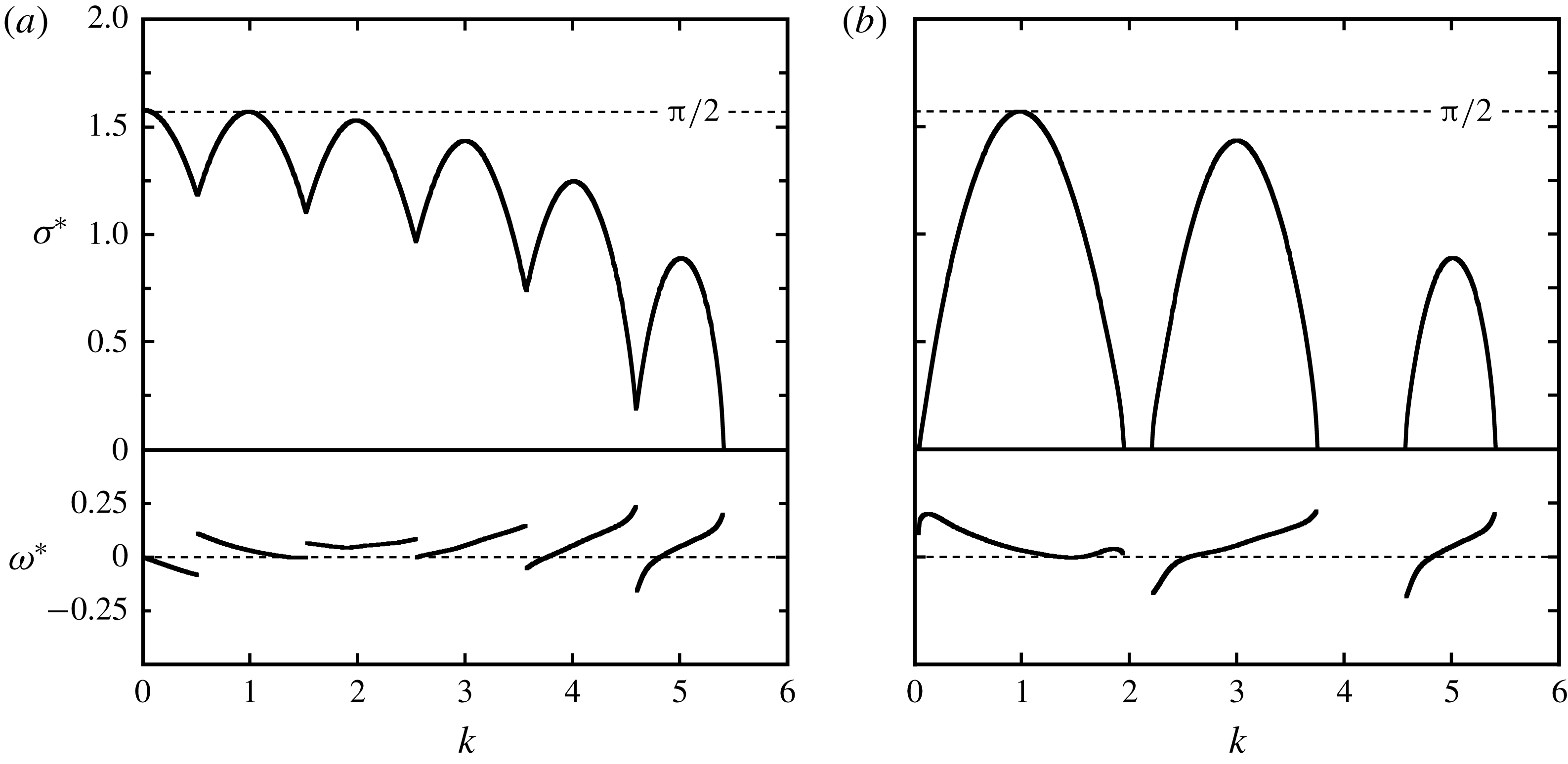
Theoretical growth rate (
 $\unicode[STIX]{x1D70E}^{\ast }$
) and frequency (
 $\unicode[STIX]{x1D714}^{\ast }$
) of the long-wave instability of two helical Rankine vortices with
 $h/R=0.41$
and
 $a_{e}/R=0.05$
, as predicted by Gupta & Loewy (Reference Gupta and Loewy1974). (a) Without fixed phase correlation between the two vortices. (b) For perturbations having the same phase at each
 $z$
(
 $\unicode[STIX]{x1D711}=0$
). Frequencies are shown only for unstable modes with the highest growth rate.

The evolution of the filaments’ shapes is obtained by computing their mutually and self-induced velocities from the Biot–Savart law. For two thin-cored vortices with circulation
 $\unicode[STIX]{x1D6E4}$
, the velocity
 $\boldsymbol{u}$
induced at a point
 $\boldsymbol{r}_{0}$
in the domain is given by
 $$\begin{eqnarray}\boldsymbol{u}(\boldsymbol{r}_{0})=-\frac{\unicode[STIX]{x1D6E4}}{4\unicode[STIX]{x03C0}}\mathop{\sum }_{m=1}^{2}\int \frac{[\boldsymbol{r}_{0}-\boldsymbol{r}(l_{m})]\times \text{d}\boldsymbol{l}_{m}}{|\boldsymbol{r}_{0}-\boldsymbol{r}(l_{m})|^{3}},\end{eqnarray}$$
in which
 $l_{m}$
is the curvilinear coordinate along the
 $m$
th vortex, whose centreline is described by
 $\boldsymbol{l}_{m}$
. For points on either one of the centrelines, the corresponding integral diverges. It can be desingularised either through a cutoff method (Crow Reference Crow1970; Widnall Reference Widnall1972), where the singularity is excluded from the integration, or by adding an appropriately chosen finite constant in the denominator (Rosenhead Reference Rosenhead1930; Moore Reference Moore1972; Gupta & Loewy Reference Gupta and Loewy1974). Both the cutoff distance and the constant depend on the core size and the velocity distribution within the core. Details can be found, for example, in Saffman (Reference Saffman1992).
By linearising the evolution equations, based on (2.6), for the two helical filaments with displacement perturbations of the form (2.5), an eigenvalue problem is obtained for the complex growth rate
 $\unicode[STIX]{x1D6FC}$
and the corresponding eigenvectors
 $\unicode[STIX]{x1D6FF}\hat{\boldsymbol{r}}_{m}$
, which represent the mode shapes, as a function of the wavenumber
 $k$
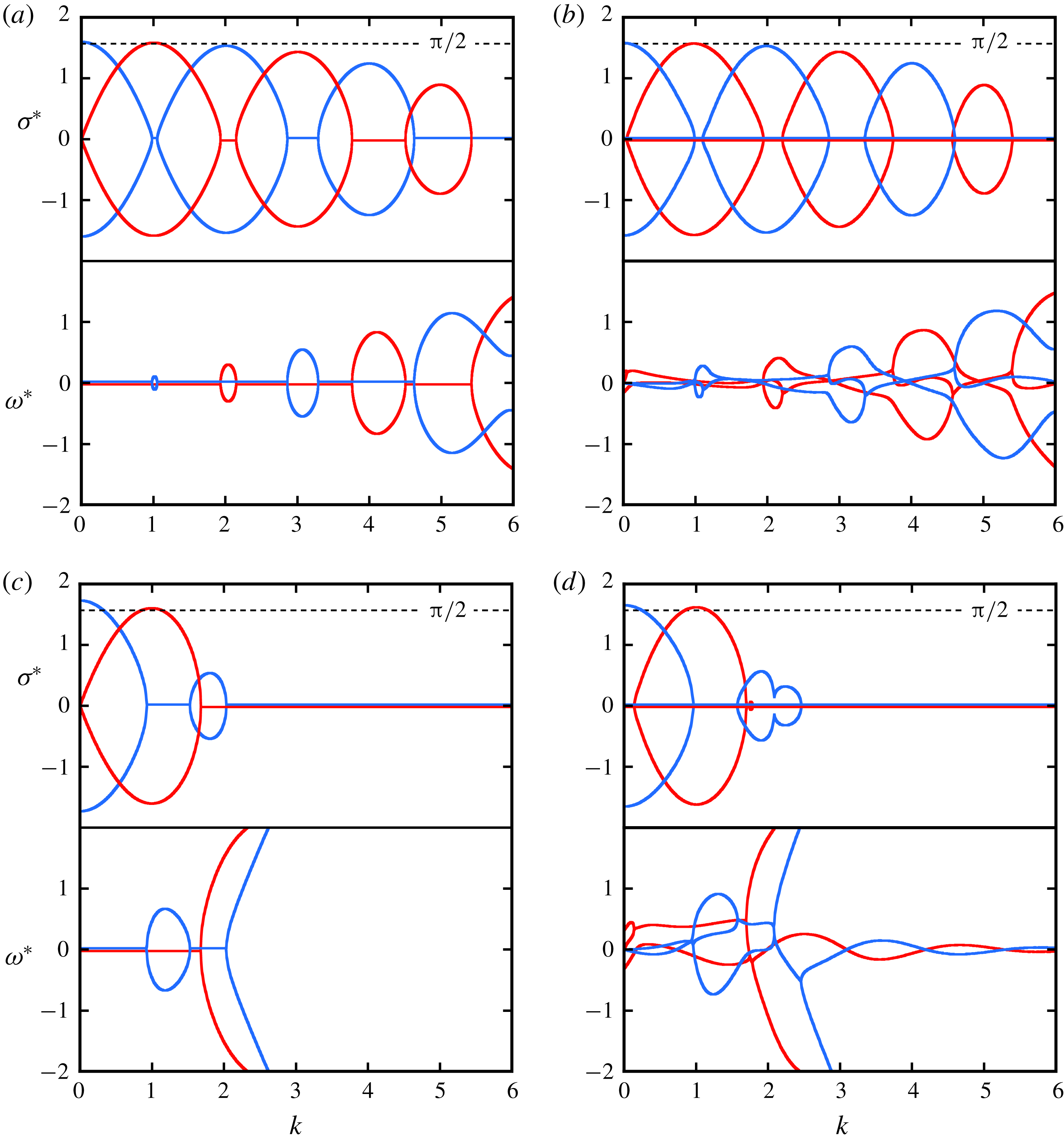
. Figure 2(a) shows a typical theoretical growth-rate curve
 $\unicode[STIX]{x1D70E}^{\ast }(k)$
and the corresponding frequencies
 $\unicode[STIX]{x1D714}^{\ast }(k)$
, calculated with the formalism of Gupta & Loewy (Reference Gupta and Loewy1974) for the flow parameters corresponding to the reference configuration in our experimental study (see § 4). The growth rate has local maxima at integer values of
 $k$
, including
 $k=0$
. The highest values are close to
 $\unicode[STIX]{x03C0}/2$
. The unstable modes include both in-phase and out-of-phase perturbations (see also figure 7 below). When the phase difference
 $\unicode[STIX]{x1D711}$
is forced to be zero, the lobes around even values of
 $k$
disappear from the growth-rate curve, and one obtains the result shown in figure 2(b). This is relevant for the experimental case, when the perturbations are triggered by a modulation of the rotor rotation (see § 3): for a rigid two-bladed rotor, these perturbations are necessarily in phase for the two vortices. The frequencies of the most unstable modes are zero or close to zero, indicating that these perturbations are steady or only slowly oscillating in time.
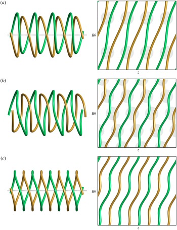
Geometrical deformation and local paring predicted by Gupta & Loewy (Reference Gupta and Loewy1974) for the case
 $h/R=0.45$
. (a) For
 $k=1$
, perturbations on both vortices are in phase at each
 $z$
. (b) For
 $k=2$
, perturbations are out of phase. (c) In-phase perturbations with
 $k=2$
, no pairing occurs. Three-dimensional views on the left and developed plan views on the right. The vertical direction of the plan views is compressed by a factor of 2.

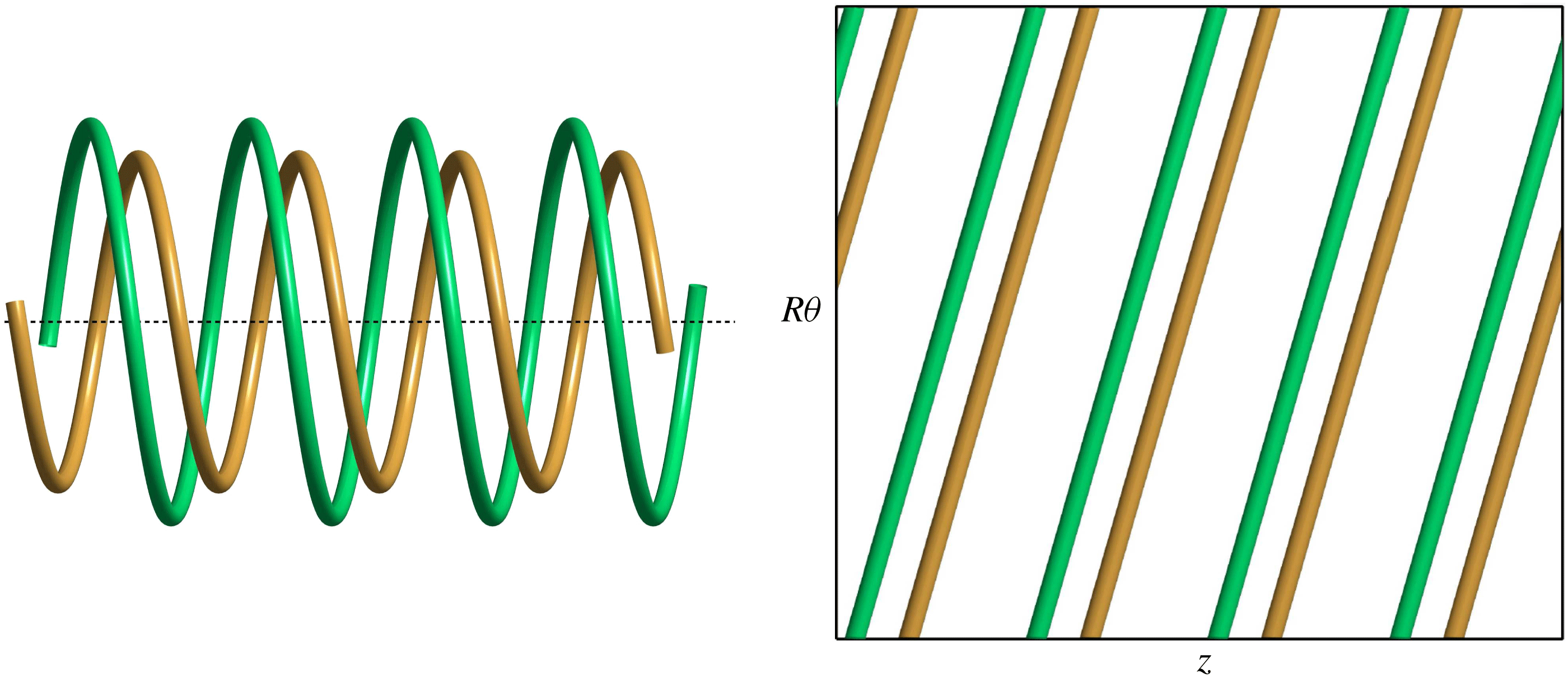
Theoretical perturbation mode for global pairing (
 $k=0$
); three-dimensional and developed plan views.

The spatial structure of the unstable deformation modes can be seen in figure 3 for the first two maxima of the growth-rate curve with non-zero
 $k$
. The deformations are in phase for
 $k=1$
and out of phase for
 $k=2$
. They result in a local pairing of successive vortex loops at
 $2k$
locations around the azimuth, as highlighted by the shaded circles in the developed plan views. Figure 3(c) illustrates that an in-phase perturbation with
 $k=2$
does not lead to local pairing of neighbouring vortex elements, which explains why
 $\unicode[STIX]{x1D70E}^{\ast }(k=2)$
vanishes in figure 2(b). The same is true for in-phase deformations at all even values of
 $k$
.
Maximum growth rate for global paring (
 $k=0$
), as a function of the relative vortex separation
 $h/R$
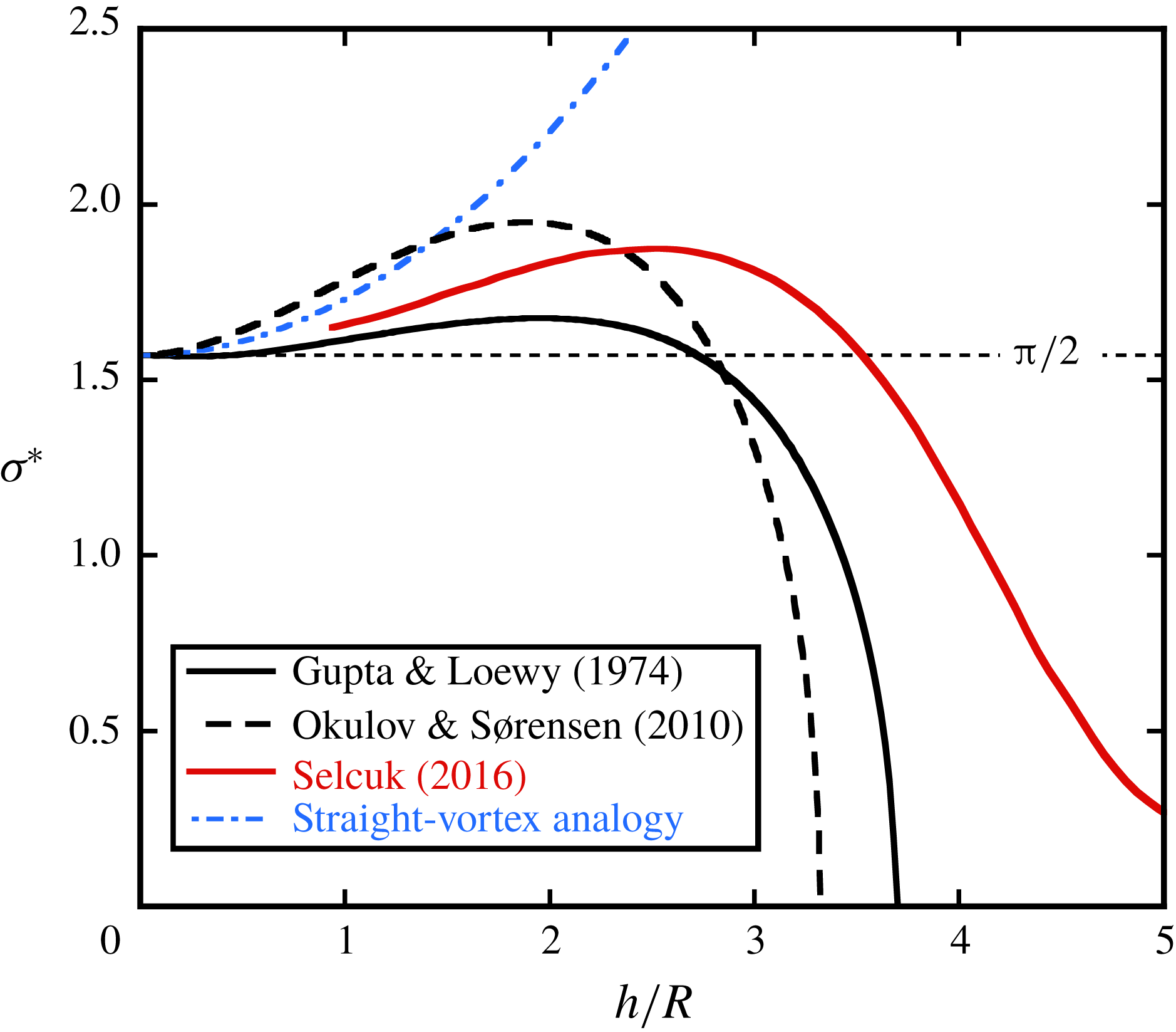
; comparison of various theoretical results. The analytical studies of Gupta & Loewy (Reference Gupta and Loewy1974) and Okulov & Sørensen (Reference Okulov and Sørensen2010) consider helical Rankine vortices, whereas Selçuk (Reference Selçuk2016) determines the stability of helical Lamb–Oseen vortices numerically. The equivalent core size is
 $a_{e}/R=0.12$
for all cases. The straight-vortex analogy corresponds to (2.7).

A special kind of unstable perturbation corresponds to the wavenumber
 $k=0$
. As shown in figure 4, it is out of phase and involves a radial expansion of one helix and a contraction of the other one, resulting in a pairing that is uniform in the azimuthal direction
 $\unicode[STIX]{x1D703}$
of the flow. In figure 5, various theoretical predictions for the growth rate of this uniform (or global) pairing, as a function of the pitch parameter
 $h/R$
, are collected and compared. All have in common that they tend to
 $\unicode[STIX]{x1D70E}^{\ast }=\unicode[STIX]{x03C0}/2$
for
 $h/R\rightarrow 0$
, and that the growth rate initially increases with
 $h/R$
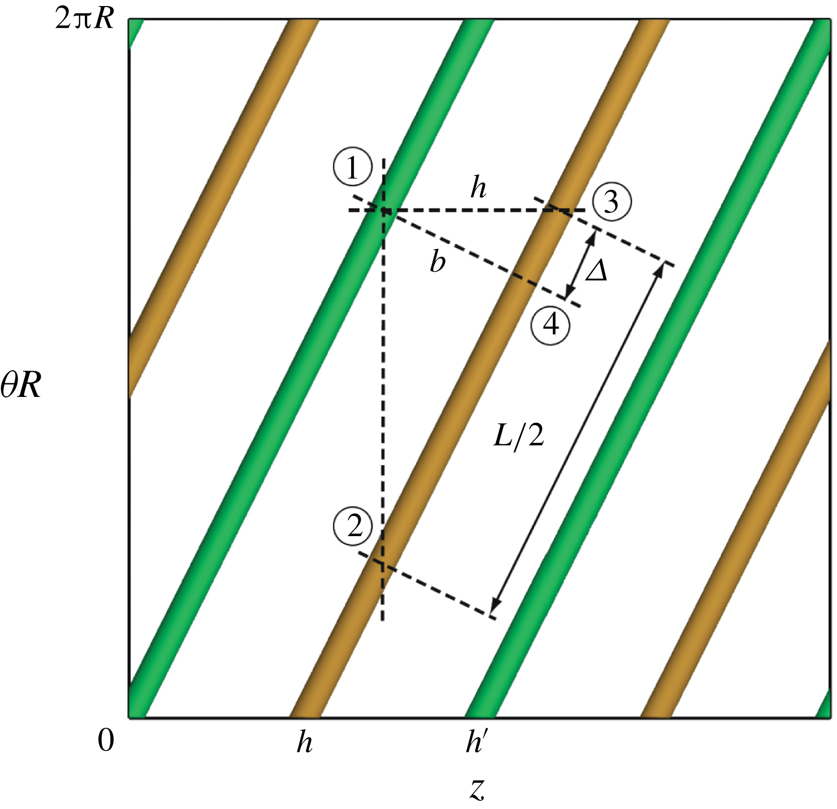
. This can partly be understood by considering an analogy with arrays of straight vortices, as depicted in the developed plan views of figure 6. The relevant length scale for the pairing instability in these systems is the shortest distance between the vortices (b in figure 6), which is smaller than
 $h$
. From simple geometry one can obtain the corresponding ‘corrected’ expression for the growth rate in the two-helix system as
 $$\begin{eqnarray}\unicode[STIX]{x1D70E}^{\ast }=\frac{\unicode[STIX]{x03C0}}{2}\left[1+\frac{1}{\unicode[STIX]{x03C0}^{2}}\left(\frac{h}{R}\right)^{2}\right],\end{eqnarray}$$
which is plotted as the dash-dotted line in figure 4. This prediction neglects the curvature of the vortices, and it is seen that the results taking into account the full three-dimensional structure of the vortex system rapidly deviate from this simple approach for increasing
 $h/R$
. In the following section, the straight-vortex-array analogy is further explored also for the local pairing of two helical vortices.
Schematic of the developed plan view of the double helix, with the definitions of the parameters employed in the analysis.

2.3 Pairing instability
In Quaranta et al. (Reference Quaranta, Bolnot and Leweke2015), a link was established between the (local) pairing instability of a single helical vortex and the pairing of an array of point vortices in two dimensions (Lamb Reference Lamb1932), which represent straight parallel vortices in three dimensions. We here refine this comparison by extending it to the theory of three-dimensional stability of vortex arrays developed by Robinson & Saffman (Reference Robinson and Saffman1982), and apply it to the two-helix system. Following Lamb (Reference Lamb1932), Robinson & Saffman (Reference Robinson and Saffman1982) considered a row of identical Rankine vortices (circulation
 $\unicode[STIX]{x1D6E4}$
, core size
 $a_{e}$
, separation distance
 $l_{RS}$
), sinusoidal displacement perturbations with a wavenumber
 $k_{RS}$
along the vortex centrelines, and a phase difference
 $\unicode[STIX]{x1D6F7}$
between neighbouring vortices. They determine the growth rate of the three-dimensional pairing instability, non-dimensionalised by
 $\unicode[STIX]{x1D6E4}/(2\unicode[STIX]{x03C0}l_{RS}^{2})$
, as a function of the base flow and perturbation parameters. As for the pairing of straight vortices (
 $k_{RS}=0$
) studied by Lamb (Reference Lamb1932), the growth rate is highest for out-of-phase perturbations (
 $\unicode[STIX]{x1D6F7}=\unicode[STIX]{x03C0}$
) between neighbours, but its value decreases with increasing wavenumber
 $k_{RS}$
.
We can transpose this result to the case of two interlaced helical vortices by considering the developed plan view in figure 6, where the system appears as a periodic array of inclined straight vortices. From the geometrical relations in this figure, one can find the expressions of the parameters in Robinson & Saffman’s (Reference Robinson and Saffman1982) analysis as a function of the helix parameters:
 $$\begin{eqnarray}\displaystyle & \displaystyle l_{RS}=b=h\frac{2\unicode[STIX]{x03C0}R}{L}=hG^{-1/2}, & \displaystyle\end{eqnarray}$$
 $$\begin{eqnarray}\displaystyle & \displaystyle k_{RS}=\frac{2\unicode[STIX]{x03C0}k}{L}=\frac{k}{R}G^{-1/2}, & \displaystyle\end{eqnarray}$$
with
 $G=1+(h/R)^{2}/\unicode[STIX]{x03C0}^{2}$
.
 $\unicode[STIX]{x1D6F7}$
is the phase shift between points
 $\unicode[STIX]{x2460}$
and
 $\unicode[STIX]{x2463}$
in figure 6. It can be calculated knowing that the phase difference between
 $\unicode[STIX]{x2460}$
and
 $\unicode[STIX]{x2461}$
is
 $\unicode[STIX]{x1D711}$
(
 $=0$
or
 $\unicode[STIX]{x03C0}$
), the one between
 $\unicode[STIX]{x2461}$
and
 $\unicode[STIX]{x2462}$
is
 $\unicode[STIX]{x03C0}k$
, and the one between
 $\unicode[STIX]{x2462}$
and
 $\unicode[STIX]{x2463}$
is a fraction
 $-2\unicode[STIX]{x1D6E5}/L$
of the latter, with
 $\unicode[STIX]{x1D6E5}=2h^{2}/L$
. This leads to
 $$\begin{eqnarray}\unicode[STIX]{x1D6F7}=\unicode[STIX]{x1D711}+\unicode[STIX]{x03C0}kG^{-1}.\end{eqnarray}$$
For a given helix geometry
 $h/R$
and displacement perturbation with wavenumber
 $k$
and phase difference
 $\unicode[STIX]{x1D711}$
, the parameters
 $l_{RS}$
,
 $k_{RS}$
and
 $\unicode[STIX]{x1D6F7}$
can be obtained from (2.8)–(2.10). Together with the core size
 $a_{e}$
, the non-dimensional complex growth rate
 $\unicode[STIX]{x1D6FC}_{RS}^{\ast }$
for three-dimensional pairing is then found from equations (2.24) of Robinson & Saffman (Reference Robinson and Saffman1982) and transformed into the current scaling via
 $$\begin{eqnarray}\unicode[STIX]{x1D6FC}^{\ast }=\frac{G}{\unicode[STIX]{x03C0}}\unicode[STIX]{x1D6FC}_{RS}^{\ast }.\end{eqnarray}$$
The (real) growth rates and frequencies obtained from this procedure for in-phase (
 $\unicode[STIX]{x1D711}=0$
) and out-of-phase (
 $\unicode[STIX]{x1D711}=\unicode[STIX]{x03C0}$
) perturbations of the reference configuration in the experimental study are plotted in figure 7(a). They are compared to the result from the stability analysis by Gupta & Loewy (Reference Gupta and Loewy1974) shown in figure 7(b), which takes the helical geometry of the base flow fully into account. It is quite striking that the growth rates are nearly identical. The more complex variation of the frequencies is also captured qualitatively well by the simplified model.
Predictions of the growth rate and frequency spectrum. (a,c) Based on the results for three-dimensional pairing of straight vortices by Robinson & Saffman (Reference Robinson and Saffman1982). (b,d) From the full stability analysis of the double-helix system (Gupta & Loewy Reference Gupta and Loewy1974). (a,b) For
 $h/R=0.41$
(experimental case) and (c,d) for
 $h/R=1$
. In-phase (red) and out-of-phase (blue) perturbations of the two vortices,
 $a_{e}/R=0.05$
.

The prediction in (2.11) is based on the assumption that the helical vortex system behaves locally like an array of straight vortices. The results are expected to become invalid for large helix pitch, for which the two-helix system locally tends towards a vortex pair configuration, where other instability mechanisms, such as the Crow instability (Crow Reference Crow1970) are likely to become dominant. Figure 7(c,d) shows the comparison for a larger pitch (
 $h/R=1$
, where each helical vortex has pitch
 $2R$
). The range of unstable wavenumbers decreases with increasing pitch. The straight-vortex model still predicts quite accurately the growth rates and frequencies, even if new modes start to appear in the full calculation (e.g. just above
 $k=2$
in figure 7
d).
The above analysis has shown that the growth rate of the displacement instability of interlaced helical vortices with moderate pitch and small core size can be predicted surprisingly well from the characteristics of three-dimensional pairing of arrays of straight vortices, which demonstrates that pairing is the underlying mechanism for this instability. In the next sections, an experimental study involving a two-bladed rotor is described, which allows the pairing instability to be observed in a real flow, and the theoretical predictions discussed above to be compared to measurements. The nonlinear stages occurring at later times (i.e. far downstream in the rotor wake) are also documented.
3 Experimental set-up and methods
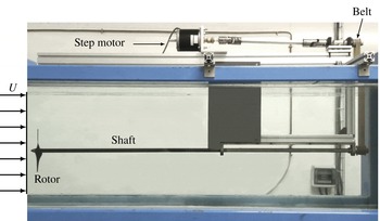
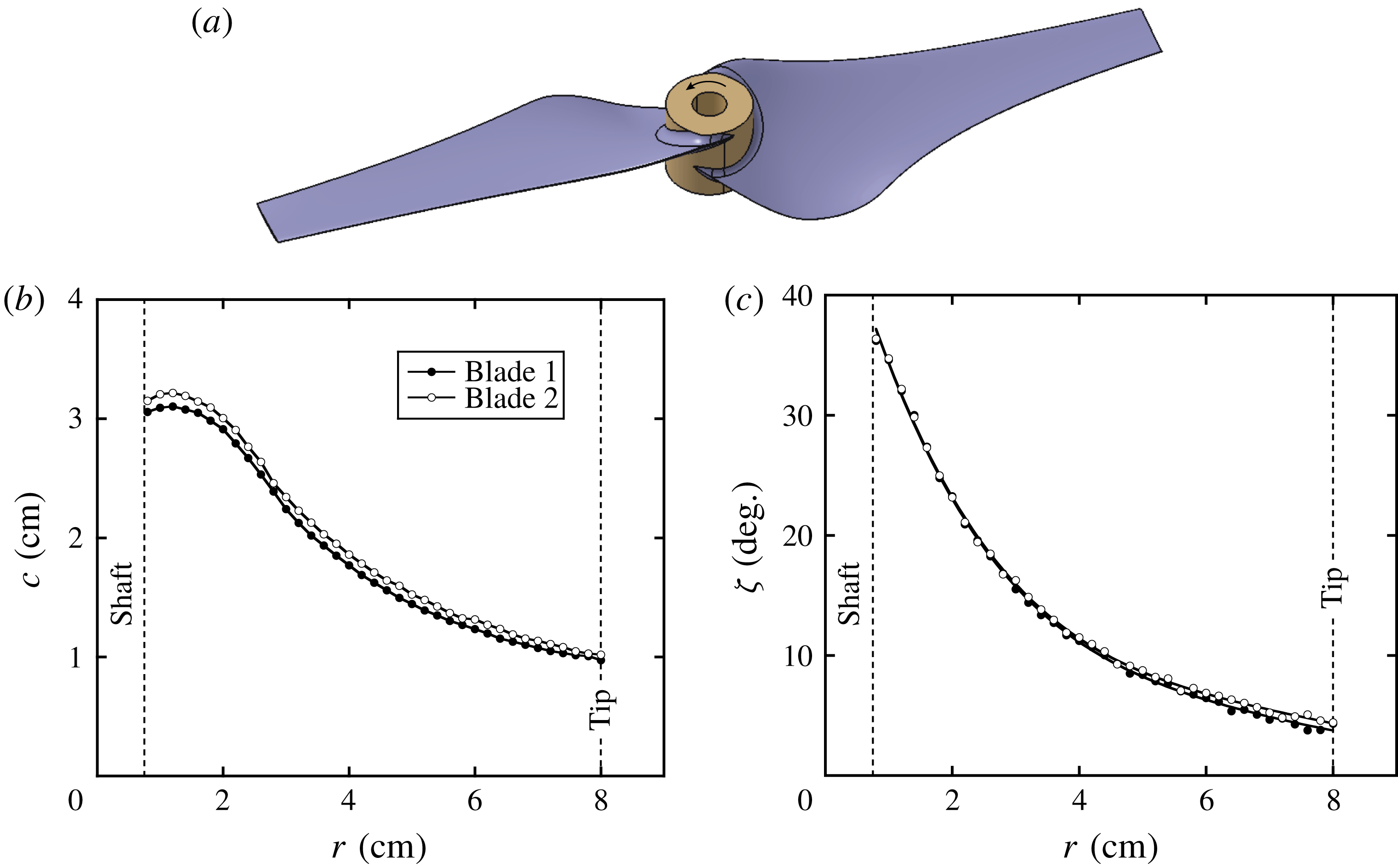
Experiments have been performed in a recirculating free-surface water channel. The set-up is similar to the one used in the work by Bolnot (Reference Bolnot2012) and Quaranta et al. (Reference Quaranta, Bolnot and Leweke2015); it is briefly described here again for completeness. The test section of the water channel (figure 8) is 150 cm long, 38 cm wide and 50 cm high. In order to generate a pair of helical vortices, a two-bladed rotor with a geometry based on the low-Reynolds-number airfoil A18 by Selig et al. (Reference Selig, Guglielmo, Broeren and Giguere1995) is used (figure 9
a). It has a radius of
 $R_{0}=80$
mm, and was designed to approximate a Joukowsky rotor with a constant radial circulation distribution over the outer 75 % of the radius. The blades have a tip chord
 $c_{tip}=10$
mm, and their chord and twist distributions are shown in figure 9.
Experimental set-up. Side view of the water channel test section.

Two-bladed rotor geometry: (a) computer-aided design (CAD) drawing, and measured radial profiles of (b) chord
 $c$
and (c) twist angle
 $\unicode[STIX]{x1D701}$
of the blades.

The rotor is mounted on a 15 mm diameter shaft equipped with an ogive tip, which is driven by a computer-controlled stepper motor. In nearly all experiments presented here, the rotation rate of the shaft is
 $f_{0}=4$
Hz. For the reference configuration, the rotor was operating in a uniform incoming flow with velocity
 $U=37~\text{cm}~\text{s}^{-1}$
, which gives a tip-chord-based Reynolds number of around 20 000 and a tip speed ratio
 $\unicode[STIX]{x1D706}=2\unicode[STIX]{x03C0}R_{0}\,f_{0}/U=5.40$
. Certain experiments were carried out at other tip speed ratios, in an interval around this value, which were obtained by varying the free-stream velocity.
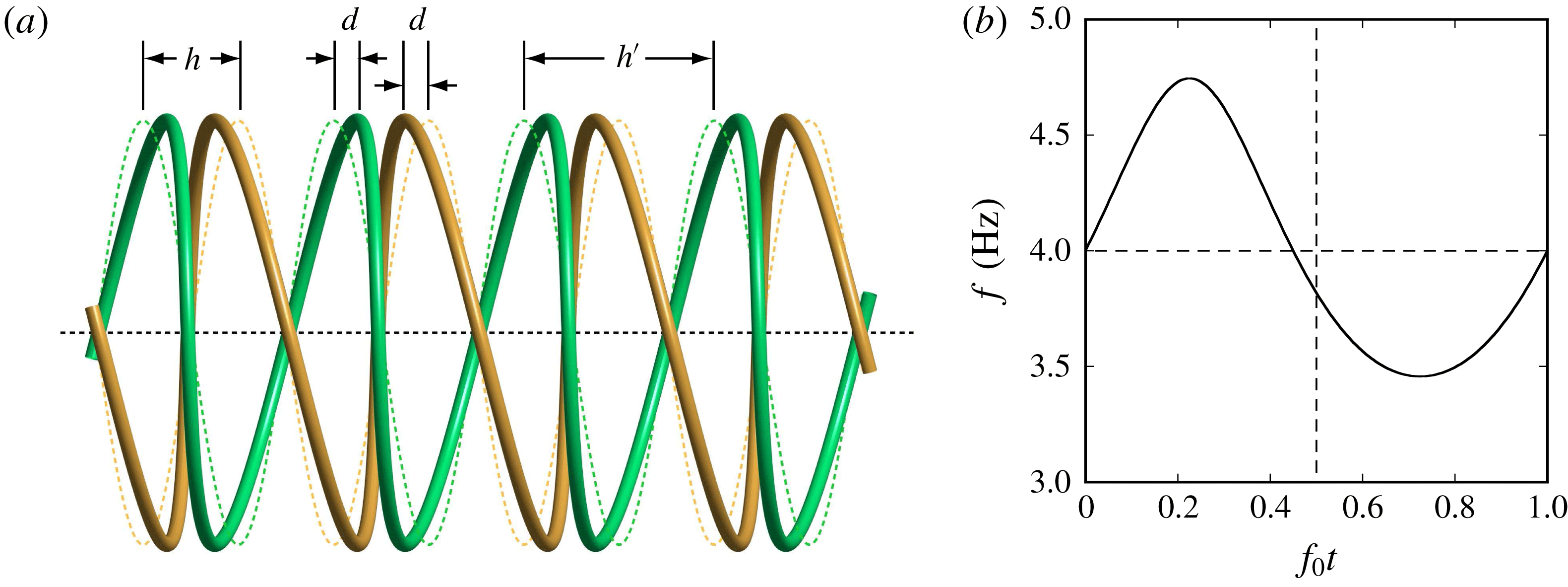
(a) Schematic of the experimental perturbation of the double helix for local pairing, consisting of an axial displacement (
 $k=1$
,
 $d/h=0.25$
). The dashed lines represent the unperturbed geometry. With a rigid rotor, only in-phase perturbations can be produced. (b) Modulation of the rotor rotation rate
 $f$
as a function of time
 $t$
, for a perturbation with
 $k=1$
and
 $d/h=0.05$
.

Local pairing is triggered by imposing controlled displacement perturbations of the two helices through periodic modulations of the blade rotation frequency
 $f$
. By varying the rotation rate, both tip vortices are simultaneously shifted in the axial direction with respect to their unperturbed positions, i.e. this shift is in phase at the same coordinate
 $z$
(see § 2.2). Considering perturbations of the type in (2.5), the
 $z$
-coordinate of the first helix (
 $m=1$
) should then have the form
 $$\begin{eqnarray}z_{p}=\frac{h^{\prime }}{2\unicode[STIX]{x03C0}}\unicode[STIX]{x1D703}+d\cos (k\unicode[STIX]{x1D703}),\end{eqnarray}$$
where
 $d$
is the amplitude. A perturbation of this type with
 $k=1$
(out-of-phase displacement of successive loops) is sketched in figure 10(a). Since the rotor moves with a velocity
 $2hf_{0}$
in the axial direction, in the frame of reference of the helical vortex, one has
 $z=2hf_{0}t$
. Differentiation with respect to time and the relation
 $\dot{\unicode[STIX]{x1D703}}=2\unicode[STIX]{x03C0}f$
lead to
 $$\begin{eqnarray}f=f_{0}\left[1-\unicode[STIX]{x03C0}k\frac{d}{h}\sin (k\unicode[STIX]{x1D703})\right]^{-1},\end{eqnarray}$$
which can be integrated numerically to obtain the rotation rate as a function of time, to be programmed into the motor controller. An example for
 $k=1$
and an amplitude
 $d/h=0.05$
is shown in figure 10(b). In this case, the frequency variation has an amplitude of approximately 15 %. As shown by Quaranta et al. (Reference Quaranta, Bolnot and Leweke2015), this seemingly large variation does not induce a significant modulation of the vortex parameters. In particular, the circulation was found to vary by only a few per cent.
(a) Schematic of a perturbed helix configuration with
 $k=0$
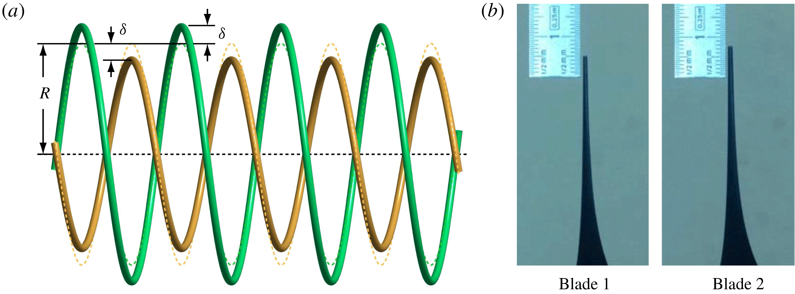
(global pairing). Two helices of slightly different radius are generated by a radial offset of the two-bladed rotor. The dashed lines indicate the unperturbed geometry. (b) Photos of the blade tips used to measure the offset.

Uniform pairing with
 $k=0$
cannot be controlled in the same way. It was instead triggered by generating two helical vortices of slightly different radius through a small radial offset of the rotor, as illustrated in figure 11. Offsets of only a few millimetres were sufficient in practice, since this mode is the most unstable pairing mode.
The vortices were visualised using two fluorescent dyes (fluorescein and rhodamine), applied to the blade tips outside the water, and subsequently illuminated by laser light. Additional visualisations were obtained by injecting dye at a fixed location in the rotor plane, in order to observe and measure the flow along the vortex cores (see figure 15 below).
Velocity fields and vorticity distributions were obtained from two-dimensional particle image velocimetry (PIV) in the centre plane of the rotor wake. These measurements were used to determine the base flow properties of the helical vortices, in particular their circulation and core size.
More details about the set-up, visualisation procedure and PIV measurements can be found in Bolnot (Reference Bolnot2012) and Quaranta et al. (Reference Quaranta, Bolnot and Leweke2015).
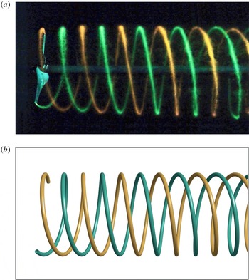
(a) Dye visualisation of the unperturbed system of two interlaced helical vortices. The rotor (radius
 $R_{0}=80$
mm) is on the left, flow is from left to right. (b) Schematic of the theoretical unperturbed base flow (uniform helices), shown in a perspective projection corresponding to the experimental observation conditions (camera located at 75 cm from the rotor shaft).

4 Unperturbed rotor wake
4.1 Base flow parameters
In this section, the properties of the undisturbed wake behind the two-bladed rotor, which corresponds to the basic state of the stability study, are discussed. This flow is visualised in figure 12(a). Although the system is unstable, the turbulence intensity in the water channel (
 ${<}1\,\%$
), the vibration levels of the rotor support and the asymmetry in the rotor geometry were sufficiently low, so that no significant perturbation of the regular helix structure could be seen in the field of observation. The latter extended for more than three rotor diameters and was limited in the downstream direction by the support structure of the shaft. The experimental helix system matches well with the theoretical base flow shown in figure 12(b) (see also figure 1).
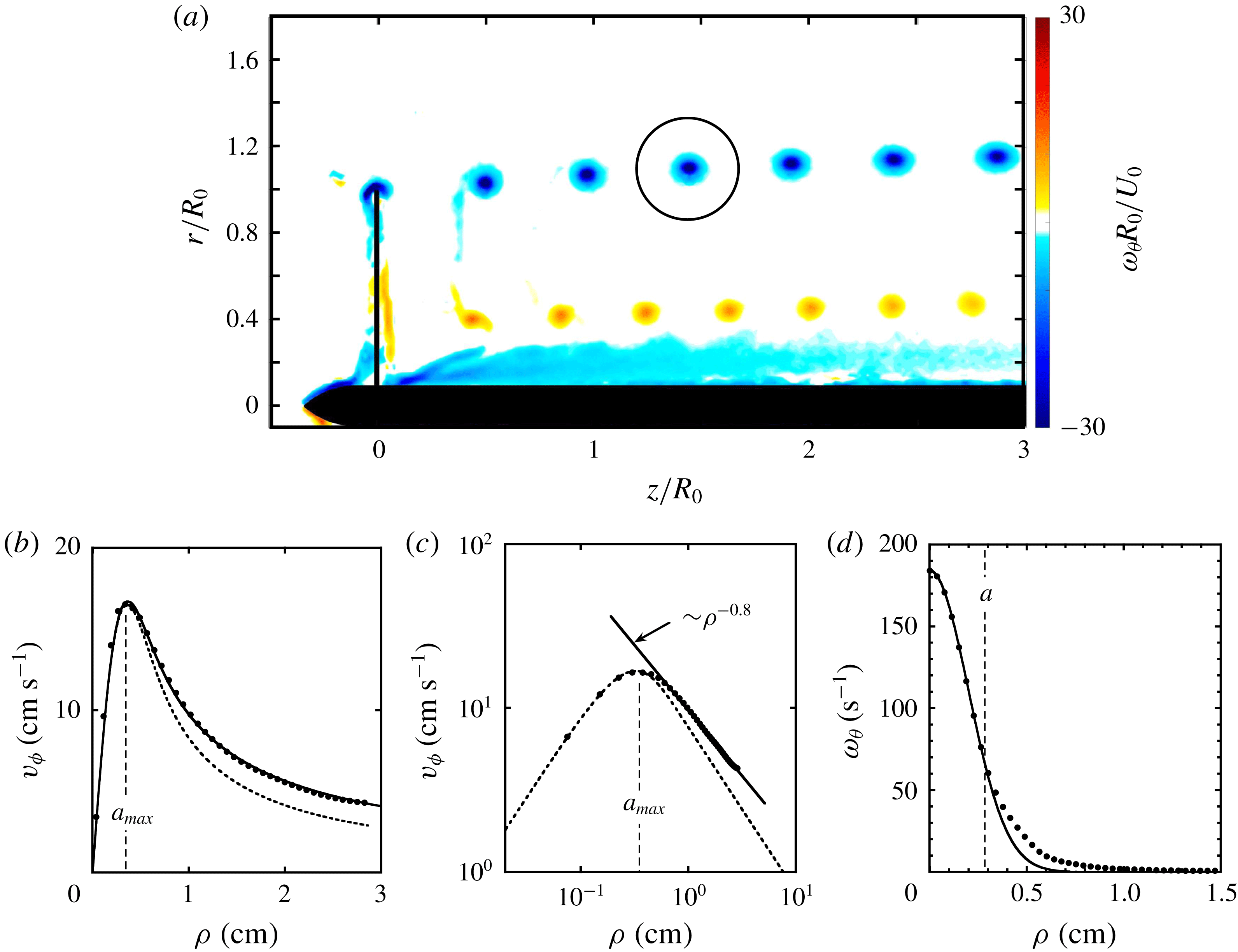
(a) Phase-averaged azimuthal vorticity field (
 $\unicode[STIX]{x1D714}_{\unicode[STIX]{x1D703}}$
) in the centre plane of the rotor, obtained from 300 PIV measurements. (b) Velocity profile of the vortex inside the circle in (a). The measurements (●) are in close agreement with the theoretical profile provided by Moore & Saffman (Reference Moore and Saffman1973) (solid line, see their equation (3.9) with
 $n=0.8$
). The dashed line represents a fit to a Gaussian profile having the same maximum. (c) Log–log plot of the velocity profile, showing that the azimuthal velocity varies as
 $\unicode[STIX]{x1D70C}^{-0.8}$
outside the core. (d) Vorticity profile of the same vortex. The line is a fit to a Gaussian distribution, using only the core data (first nine measurements).

In figure 13(a), the phase-averaged azimuthal vorticity field in the near-wake centre plane of the rotor is plotted. It clearly shows the tip vortices along with the root vortices of opposite-signed vorticity at
 $r/R_{0}\approx 0.4$
, and the boundary layer on the shaft. It is notable that the root vortices have a slightly smaller pitch than the tip vortices.
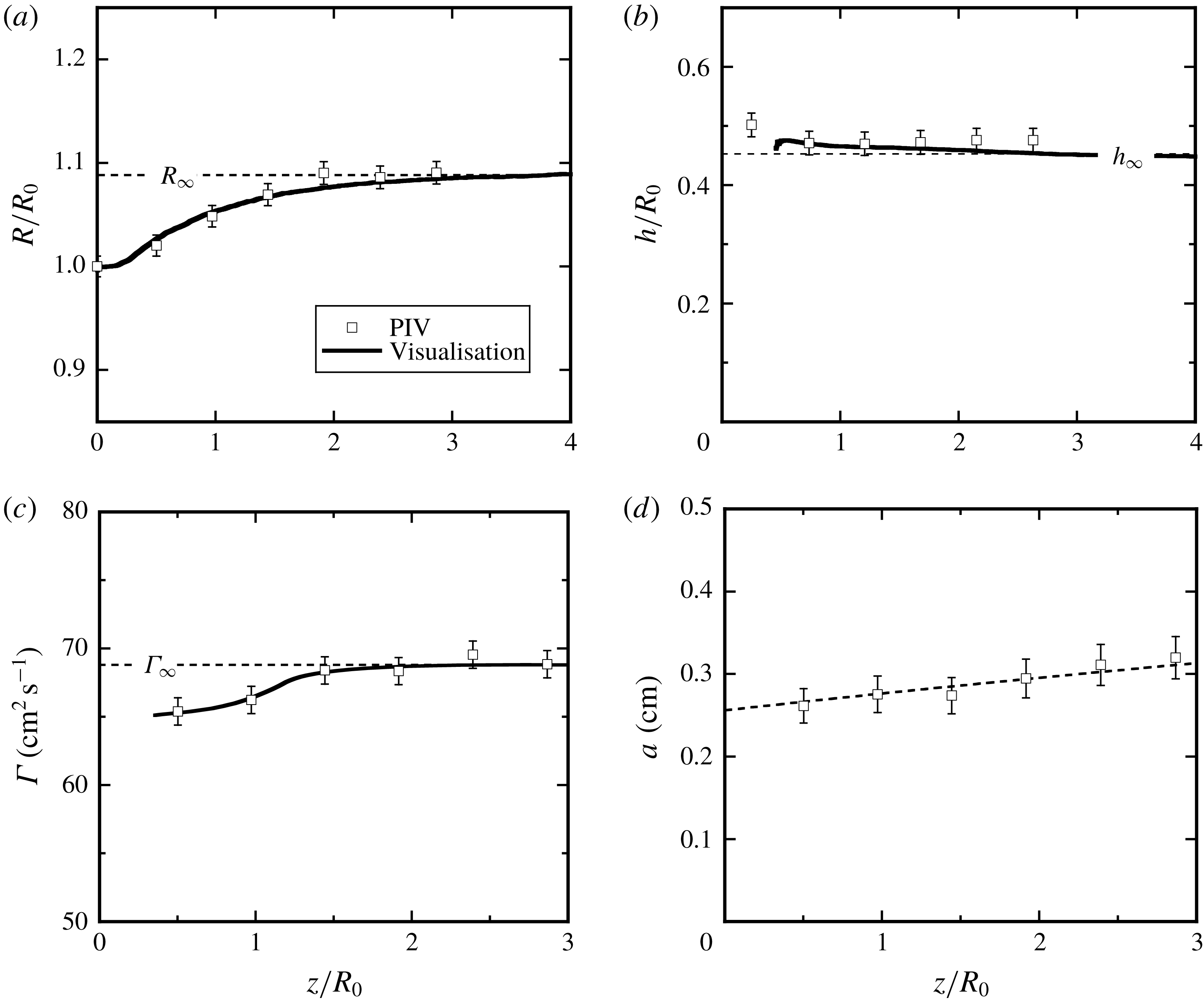
Characteristic parameters of the double-helix configuration and their downstream evolution. Geometric parameters: (a) helix radius
 $R$
and (b) separation
 $h$
between neighbouring helix loops. Vortex parameters: (c) circulation
 $\unicode[STIX]{x1D6E4}$
and (d) core size
 $a$
. The dashed line in (d) is a fit to the viscous expansion of a two-dimensional Gaussian vortex core,
 $a=\sqrt{4\unicode[STIX]{x1D708}(t-t_{0})}$
.

The radius and pitch of the tip vortex system were measured from the dye visualisations by detecting the centres of the dye loops (corresponding to the vortex cores) at the top and bottom of the helix, and tracing these throughout the wake using image-tracking software (Brown Reference Brown2017). In order to compensate for the scatter in the measurements, due partly to temporal fluctuations in the wake, several vortex ridges were traced and their corresponding trajectories averaged. The resulting helix radius and vortex separation are plotted as a function of the distance from the rotor in figures 14(a) and 14(b), respectively. As expected for a rotor operating in the wind turbine regime, the radius increases with downstream distance from the rotor plane; it reaches its asymptotic value
 $R_{\infty }$
after two to three radii. The distance between successive helix loops is around 45 % of the blade span, and varies little in the downstream direction. Considering the maxima of the azimuthal vorticity, the parameters
 $R$
and
 $h$
could also be obtained from the PIV measurements. As seen in figure 14, the outcomes of the two techniques are in good agreement with each other.
The circulation of the tip vortices was calculated from the velocity field using line integrals on circular paths of diameter
 $h$
, as shown in figure 13(a). It increases gradually over a distance of 1.5 rotor radii (figure 14
c), which is a signature of the roll-up process of the initial vortex sheet shed by the blade. The reference circulation (
 $\unicode[STIX]{x1D6E4}_{\infty }$
) for the base flow configuration is the one measured at the downstream end of the PIV field. The root vortex circulation, obtained in a similar way, is only approximately 30 % of the tip vortex circulation. This low value can be understood by considering the boundary layer developing on the rotor shaft. Owing to the zero streamwise velocity on the shaft surface, the boundary layer contains approximately twice as much circulation (per distance
 $h$
) as the tip vortices. Part of this circulation mixes with, and cancels a large fraction of, the root vortex circulation, through the complicated flow behind the rotor hub.
4.2 Vortex core velocities
The swirl velocity profile of the tip vortices was measured from the PIV data using local polar coordinates (
 $\unicode[STIX]{x1D70C},\unicode[STIX]{x1D719}$
) centred on a given vortex. Figure 13(b) shows a profile of the azimuthally averaged azimuthal velocity in these coordinates, which allows a determination of the core size
 $a_{max}$
. This profile differs from the one of a Gaussian vortex, which underestimates the velocities outside the core, indicating that the outer region also contains circulation. A better fit to the experimental data is provided by the theoretical velocity distribution given by Moore & Saffman (Reference Moore and Saffman1973) for laminar vortices resulting from the vortex sheet roll-up behind a lifting surface. In particular, the azimuthal velocity is found to vary as
 $\unicode[STIX]{x1D70C}^{-0.8}$
outside the core (figure 13
c).
Since the vortex Reynolds number is here of the order of
 $10^{4}$
, one might expect some degree of turbulence inside the vortices. Phillips (Reference Phillips1981) has calculated the velocity profiles of turbulent wing-tip vortices, which turn out to be very close to the laminar profiles of Moore & Saffman (Reference Moore and Saffman1973). The identification of the turbulent nature based on the measured swirl velocity or circulation profiles therefore seems hardly possible. In our case, the inner core region (for
 $\unicode[STIX]{x1D70C}\lesssim a_{max}$
), which has the main influence on the pairing instability, appears to be laminar, since its size increases on a time scale dictated by the molecular viscosity of the fluid (figure 14
d).
As discussed in more detail in Quaranta et al. (Reference Quaranta, Bolnot and Leweke2015), the core structure influences the self-induced velocity of the vortex through the equivalent Rankine core radius
 $a_{e}$
(see § 2.1). Theoretical work of Fabre (Reference Fabre2002) suggests that profiles with the same
 $a_{max}$
have a very similar equivalent core size, so that the development for Gaussian vortices outlined in § 2.1 also can be applied to the experimental vortices. (In addition, the instability growth rate is found to depend only weakly on the vortex core size, in the range of parameters considered in this study.) The downstream evolution of the characteristic (Gaussian) core radius
 $a\approx a_{max}/1.12$
(derived from (2.2a
)) is plotted in figure 14(d); it follows the laminar viscous growth of a Gaussian vortex fairly well. As a representative value to use in the stability calculations, the core radius near
 $z/R_{0}=2$
is chosen. The core size
 $a$
can also be obtained from the vorticity profile of the vortex (figure 13
d). For a Gaussian vortex, it is the half-width at a fraction
 $1/\text{e}$
of the maximum value. The core sizes obtained from the measured vorticity profiles, using this criterion, are roughly the same as the ones obtained from the profiles of the swirl velocity.
The tip vortex generated from the roll-up of a vortex sheet behind a wing or blade also contains an axial velocity component (along the vortex centreline), as derived by Batchelor (Reference Batchelor1964). Inside the core, the pressure is lower compared to the upstream flow, such that fluid elements entering the vortex core may experience a noticeable axial acceleration. As a result, the axial flow inside the core will behave like a jet in the frame of reference of the helix. Taking into account the effects of viscosity and the boundary layer on a wing, Moore & Saffman (Reference Moore and Saffman1973) developed a model which showed that the axial flow inside the core can be either in the same direction as the motion of the wing tip or opposite to it, depending on the load distribution of the wing, the chord and the Reynolds number.
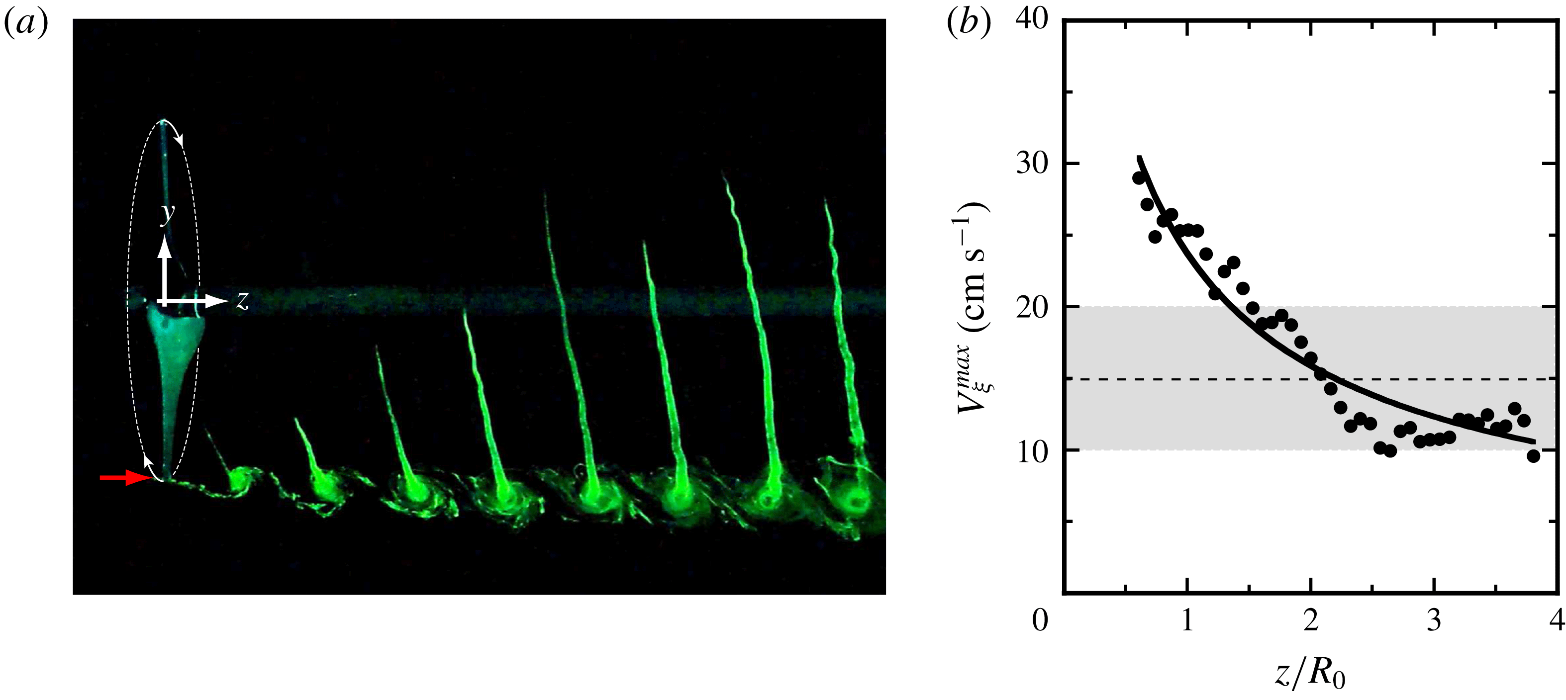
(a) Visualisation of the axial flow within the vortex cores of the undisturbed helices. The red arrow indicates the location in the rotor plane where dye is injected. (b) Peak velocity along the centreline of the vortices as a function of downstream distance. Symbols represent measurements obtained from visualisations such as in (a); the line is the prediction in (4.1) based on Moore & Saffman (Reference Moore and Saffman1973), using the measured vortex properties. The shaded range represents the values occurring during the growth-rate measurements.

In the present experiments, the axial core flow is visualised using a method similar to that used by Quaranta et al. (Reference Quaranta, Bolnot and Leweke2015), where dyed fluid is injected at a fixed location in the vicinity of the rotor plane (
 $z=0$
). As seen in figure 15(a), the dye follows the motion of the blades. In the reference frame of a blade, this motion corresponds to a velocity deficit within the cores of the tip vortices.
For the purpose of comparing with theoretical results, we assume here that the axial velocity profile may be approximated by a Gaussian profile, with a maximum velocity
 $V_{\unicode[STIX]{x1D709}}^{max}$
(2.2b
). The value of this maximum velocity, in the direction of the vortex centreline, can be estimated by tracking in time the positions of the tips of the dye pattern in figure 15(a). Several dye tip trajectories were obtained and averaged, and after a straightforward but tedious geometrical transformation and derivation, one obtains the downstream evolution of the maximum core velocity shown in figure 15(b). The figure also shows the prediction that can be derived from the model of Moore & Saffman (Reference Moore and Saffman1973) for our case. For a (straight) viscous trailing vortex with an outer velocity profile given by
 $v_{\unicode[STIX]{x1D719}}(\unicode[STIX]{x1D70C})=\unicode[STIX]{x1D6FD}/\unicode[STIX]{x1D70C}^{n}$
, their equation (3.30) predicts the maximum core velocity as
 $$\begin{eqnarray}V_{\unicode[STIX]{x1D709}}^{max}=\frac{\unicode[STIX]{x1D6FD}^{2}}{U_{s}c_{tip}^{2n}}\left(\frac{s}{c_{tip}}\right)^{-n}Re_{c}^{n}\unicode[STIX]{x1D700}_{n}-0.053\sqrt{\unicode[STIX]{x03C0}}(4-2n)U_{s}\left(\frac{s}{c_{tip}}\right)^{-1/2},\end{eqnarray}$$
where
 $U_{s}=Lf_{0}$
(see figure 6 for
 $L$
) is the blade-tip velocity with respect to the fluid,
 $Re_{c}=U_{s}c_{tip}/\unicode[STIX]{x1D708}$
the tip-chord-based Reynolds number,
 $s=(L/2h)z$
the coordinate along the vortex centreline, and
 $\unicode[STIX]{x1D700}_{n}$
a constant depending on the exponent
 $n$
. From the measured vortex velocity profile in figure 13(c) one finds
 $n=0.8$
, resulting in
 $\unicode[STIX]{x1D700}_{0.8}=-0.7$
(figure 2 of Moore & Saffman (Reference Moore and Saffman1973)). The solid line in figure 15(b) shows the resulting prediction for
 $V_{\unicode[STIX]{x1D709}}^{max}(z/R_{0})$
, where only the parameter
 $\unicode[STIX]{x1D6FD}$
and the origin for the downstream position were adjusted. The observed evolution (decrease) of the velocity defect inside the tip vortices is well captured by the model. A value representing the mean velocity during the exponential growth phase of the pairing instability is kept for comparison with theory (see table 1). This velocity has approximately the same magnitude as the maximum swirl velocity (see figure 13
b) and corresponds to approximately 7 % of the blade-tip speed.
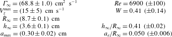
Experimentally determined flow parameters of the unperturbed vortex system.

The base flow properties and the non-dimensional parameters for the system of two interlaced helical vortices in our experimental rotor wake are summarised in table 1. Uncertainties are based on the scatter of the individual measurements, and on estimates of the accuracy of the measurement procedures.
5 Pairing instabilities
5.1 Local pairing
When the symmetrically mounted rotor is rotating at a constant rate, the helix structures generated in its wake do not show any significant deformation over the first three diameters behind the rotor (figure 12). However, when slightly modulating the rotation frequency, as outlined in § 3, displacement perturbations are introduced that rapidly amplify and distort the vortex as it advects downstream, demonstrating the instability of the system with respect to such perturbations.
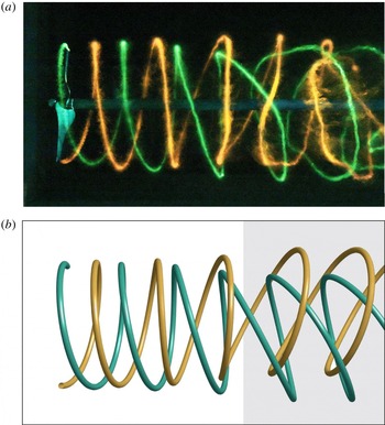
Rotor wake perturbed with a local pairing mode (
 $k=1$
). (a) Experimental dye visualisation for
 $d/h_{\infty }=0.05$
; (b) corresponding theoretical prediction (the perturbation amplitude is kept constant in the grey region).

Figure 16(a) shows a dye visualisation of the perturbation mode
 $k=1$
, triggered with an initial displacement of amplitude
 $d/h_{\infty }=0.05$
. This mode corresponds to the first maximum of the in-phase perturbation growth-rate curve in figure 2(b). At the two azimuthal locations where the displacement of the vortex filaments is the largest, local pairing occurs. The phase of the blade rotation modulation was chosen such that this happens at the top and bottom in the view of figure 16(a). Figure 16(b) presents the corresponding theoretical shape from the stability analysis. The temporal growth from the theory is transformed into a spatial growth relevant for the rotor geometry using the vortex convection speed
 $2hf_{0}$
and an appropriately chosen initial perturbation amplitude and phase. The experimental and theoretical structures agree very well, approximately up to the point where consecutive vortex loops are displaced to the same downstream position (at
 $z/R_{0}\approx 3$
, near the centre of the figure), which marks the end of the linear regime of the pairing instability (see also § 6).
Schematic illustrating the displacement of the vortex cores in the upper half of the centre plane due to local pairing. The distances
 $d_{1}$
and
 $d_{2}$
are used to estimate the growth rate of the perturbation. (a) Unperturbed and (b) perturbed configuration.

The growth rate of the instability was determined from visualisation sequences, for various perturbation wavenumbers
 $k$
. Every sequence contained an initial phase of unperturbed flow (figure 12), which served as the reference configuration, followed by a phase where the flow was perturbed with the rotation modulation (figure 10
b). The positions of the upper and lower sections of the vortex loops for the unperturbed and perturbed flows were measured using tracking software (Brown Reference Brown2017), and the distances between them (marked as
 $d_{1}$
and
 $d_{2}$
in figure 17
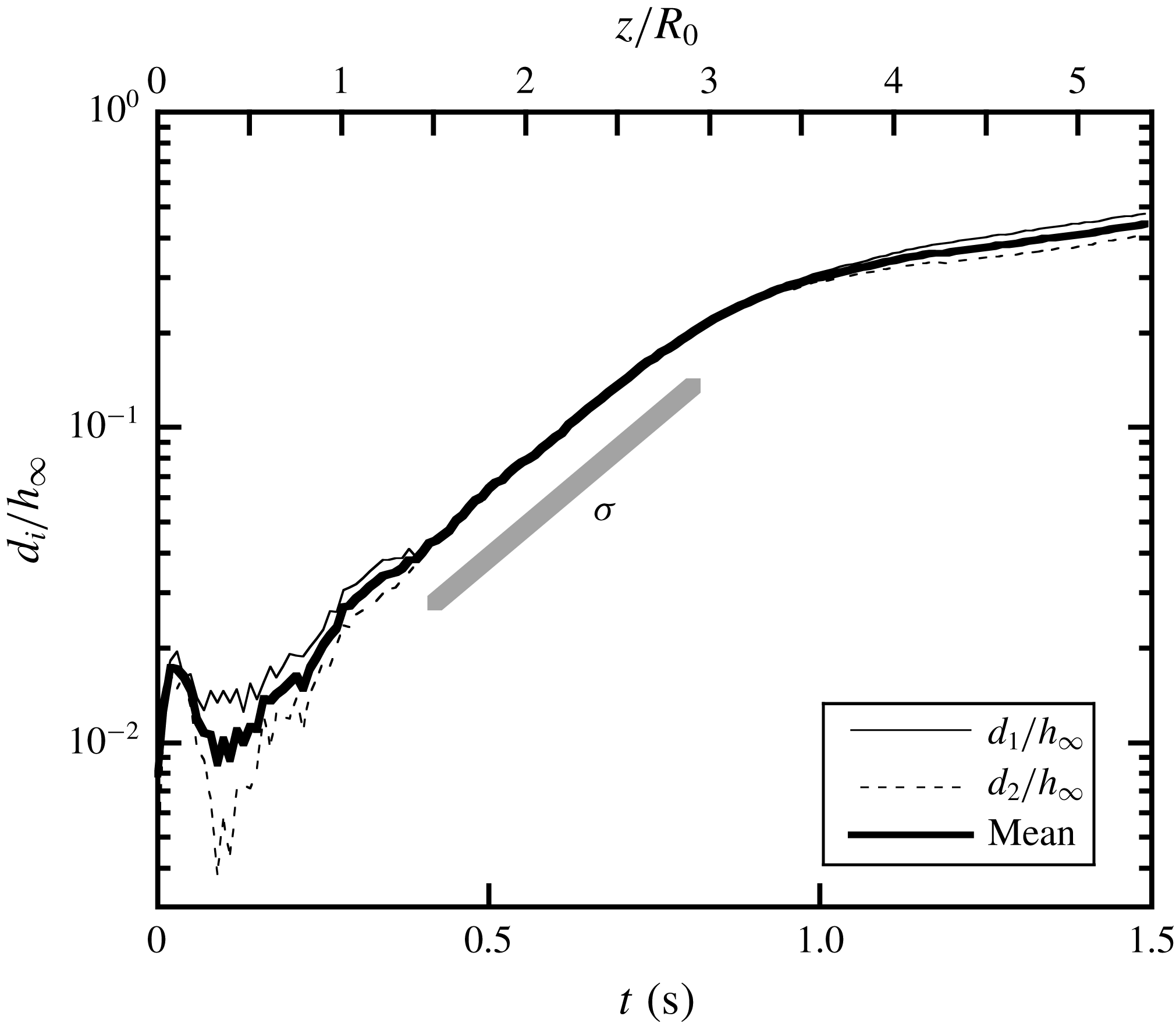
b) were calculated as a function of time. Multiple individual measurements were made for each case, in order to obtain the average trajectories with precision. Figure 18 shows a typical example of the resulting amplitude evolution, from which the linear growth rate can easily be determined.
Averaged temporal evolution of the displacement amplitudes
 $d_{i}$
(
 $i=1,2$
), defined in figure 17(b), for a perturbation with
 $k=1$
and
 $d/h_{\infty }=0.03$
. The slope of the thick grey line gives the growth rate
 $\unicode[STIX]{x1D70E}$
.

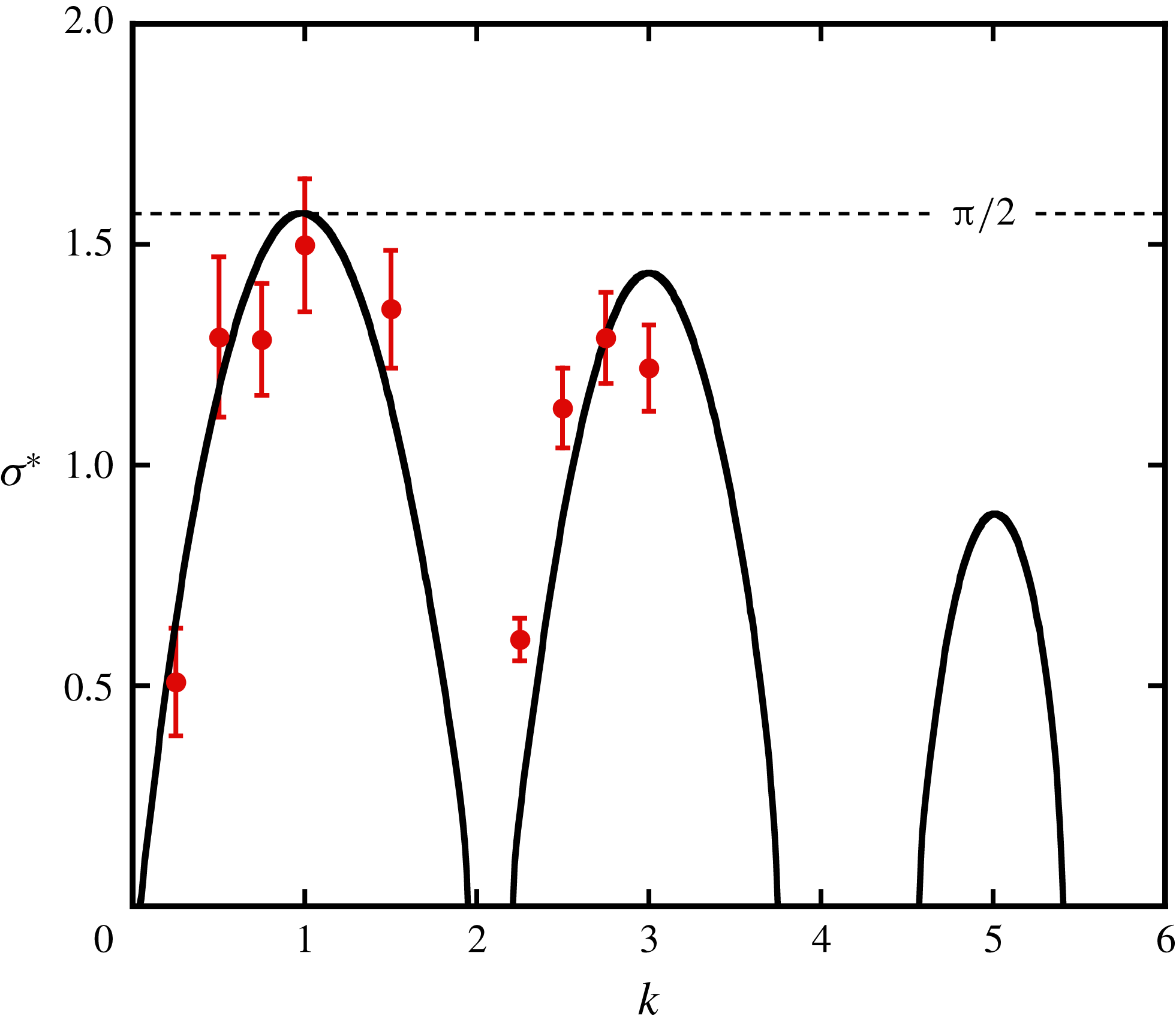
Growth rate of the long-wave instability due to local pairing, as a function of wavenumber. The symbols correspond to experimental measurements, and the solid line is the theoretical prediction by Gupta & Loewy (Reference Gupta and Loewy1974) for in-phase perturbations on the two vortices. The theoretical results are obtained using the base flow parameters in table 1.

The growth rates for local pairing were measured for various azimuthal wavenumbers in the range
 $0<k<4$
. In each experiment, it was verified visually that the amplified perturbation was indeed the one corresponding to the imposed wavenumber. In certain cases with off-maximum wavenumbers, the perturbation eventually dominating in the visualisation could have a different wavenumber than intended, with a higher growth rate. Whenever there was a doubt, the measurements were discarded. Figure 19 shows all the valid growth rates that could be obtained in our experiments, as a function of wavenumber. The comparison with the theoretical predictions for in-phase perturbations, using the base flow parameter values corresponding to our experimental configuration, shows good agreement.
5.2 Global pairing
As seen in § 2.2 (figure 7), a system of two interlaced helical vortices is also unstable with respect to displacement perturbations that are out of phase. With the current set-up using a rigid rotor, the only out-of-phase perturbation that could be imposed is the one with
 $k=0$
, without modulation of the rotor frequency (any such modulation would again result in an in-phase perturbation). As explained in § 3, such a perturbation could be obtained by introducing a small radial offset of the rotor (typically a few per cent of
 $R_{0}$
), resulting in the generation of two helical vortices of slightly different radii undergoing uniform pairing (figure 4). In order to explore the variation of the growth rate for global pairing with the helix geometry (
 $h/R$
, figure 5), four different tip speed ratios
 $\unicode[STIX]{x1D706}$
were used by varying the free-stream velocity in the water channel. For each case, the base flow parameters (helix geometry
 $R$
and
 $h$
; vortex properties
 $\unicode[STIX]{x1D6E4}$
and
 $a$
) were determined as described in § 4.1.
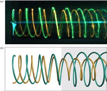
Rotor wake perturbed with a global pairing mode (
 $k=0$
). (a) Experimental dye visualisation for the case with tip speed ratio
 $\unicode[STIX]{x1D706}=5.40$
and radial rotor offset
 $\unicode[STIX]{x1D6FF}/R_{0}=0.015$
. (b) Corresponding theoretical prediction (the perturbation amplitude is kept constant in the grey region).

Figure 20(a) shows a visualisation of global pairing, obtained with the reference configuration (
 $\unicode[STIX]{x1D706}=5.40$
) and a rotor offset
 $\unicode[STIX]{x1D6FF}/R_{0}=0.015$
. Pairing occurs simultaneously around the azimuth of the rotor, and the agreement of the spatial structure with the prediction derived from theory is again very good, up to the location of vortex loop swapping at around
 $z/R_{0}=3$
. Beyond this point, the rotor wake system almost returns to its initial configuration. The late stages of the global pairing instability are further analysed in § 6.
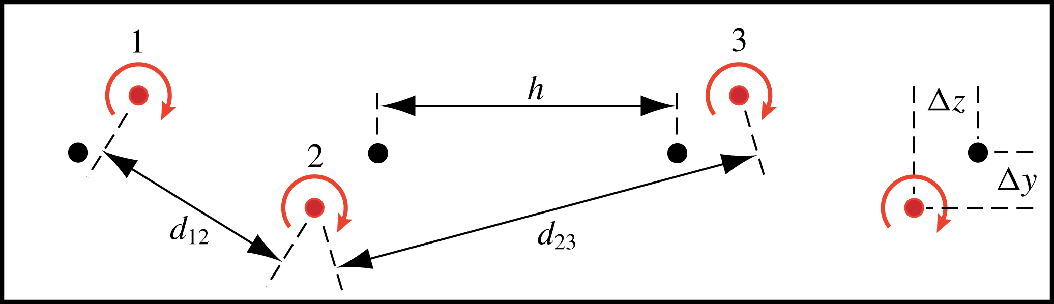
The growth rate of the uniform pairing mode was again determined from video recordings of dye visualisations. Unlike the case with local pairing, these videos had no initial sequence with unperturbed flow, since the rotor offset could only be set in advance. Therefore a different post-processing method was used, similar to the one presented in Bolnot (Reference Bolnot2012). In this method, a group of three consecutive vortex ridges is followed throughout the wake, and their corresponding trajectories determined with the same image tracking software as used before (Brown Reference Brown2017). Figure 21 illustrates this configuration. Assuming a temporal development of the pairing instability that is uniform along the vortex array, and using the fact that for
 $k=0$
the perturbations of neighbouring vortices are out of phase, it is straightforward to show that
 $d_{23}^{2}-d_{12}^{2}=8h\unicode[STIX]{x0394}z$
. In the linear regime of the instability, the distances
 $\unicode[STIX]{x0394}y$
and
 $\unicode[STIX]{x0394}z$
increase exponentially in time with growth rate
 $\unicode[STIX]{x1D70E}$
, just like the distances
 $d_{1}$
and
 $d_{2}$
in figure 17. This means that the temporal evolution of the difference
 $d_{23}^{2}-d_{12}^{2}$
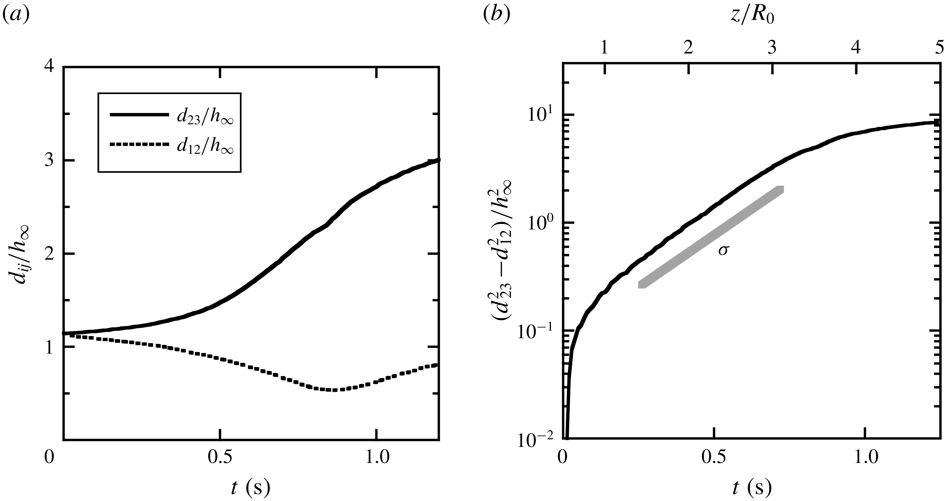
can be used to determine the pairing instability growth rate directly from the perturbed configuration, without knowledge of the unperturbed vortex positions. An example of such a measurement is shown in figure 22.
Schematic illustrating the displacement of the perturbed vortex cores in the upper half of the centre plane. The distances
 $d_{12}$
and
 $d_{23}$
are used to estimate the growth rate of the perturbation. The unperturbed and perturbed vortex positions are marked with black and coloured bullets, respectively.

Growth of the global pairing instability (
 $k=0$
), as measured in the upper wake cross-section for
 $\unicode[STIX]{x1D706}=5.40$
. (a) Averaged temporal evolution of
 $d_{12}$
and
 $d_{23}$
defined in figure 21. (b) The difference
 $d_{23}^{2}-d_{12}^{2}$
, whose exponential increase yields the instability growth rate
 $\unicode[STIX]{x1D70E}$
. The time
 $t=0$
marks the instant when the vortex labelled 1 in figure 21 is shed from the blade tip. The upper horizontal axis indicates the corresponding
 $z$
-position of the ‘second’ vortex loop (labelled 2).

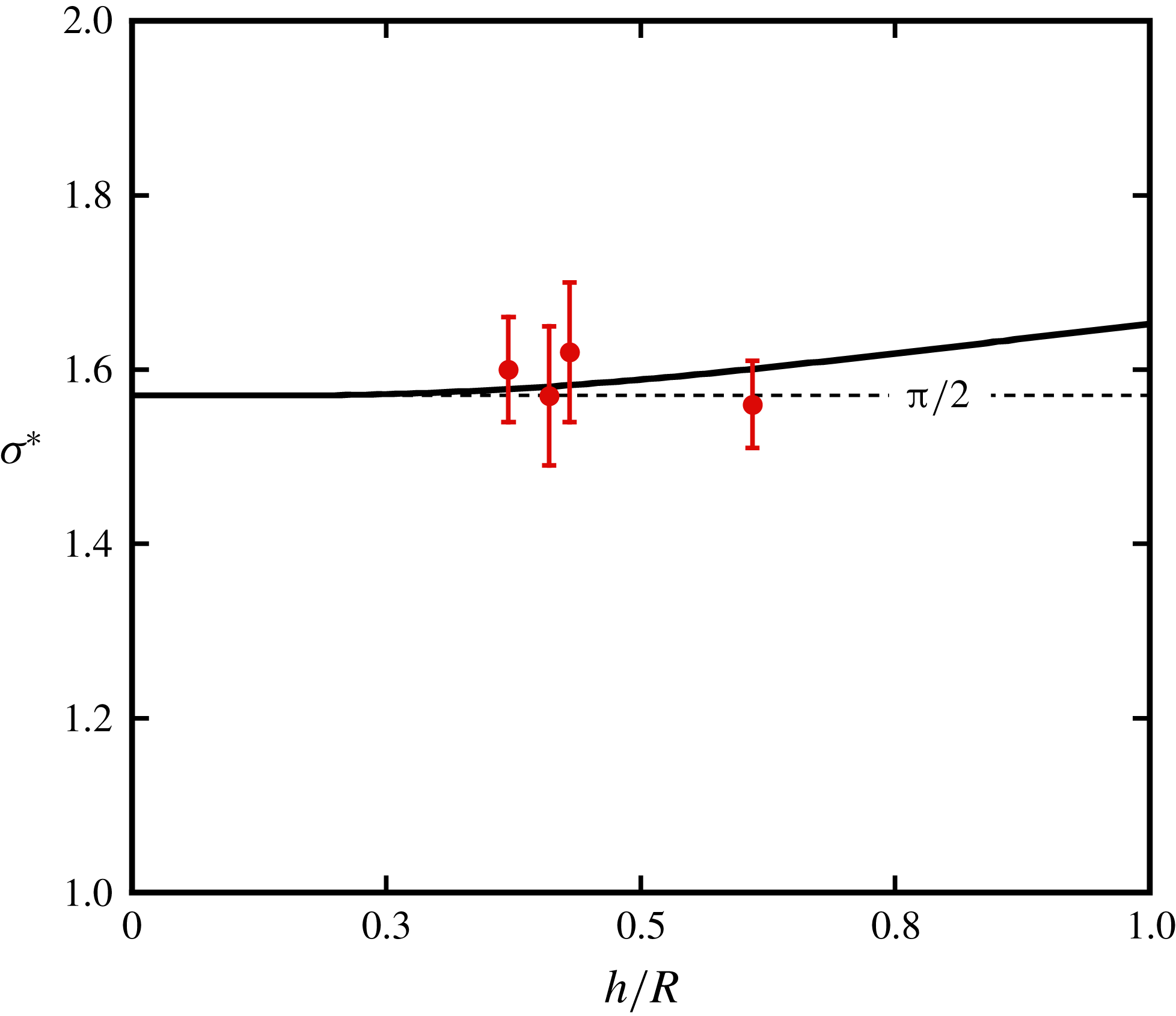
Growth rate of the long-wave instability due to global pairing, as a function of the distance between neighbouring helix loops. Symbols correspond to experimental measurements, and the solid line is the theoretical prediction by Gupta & Loewy (Reference Gupta and Loewy1974) for
 $a_{e}/R=0.05$
.

The resulting growth rates for tip speed ratios
 $\unicode[STIX]{x1D706}=4.47,~5.40,~6.67$
and 8.04 are plotted in figure 23 as a function of the corresponding parameter
 $h/R$
. They are compared to the theoretical prediction based on the work of Gupta & Loewy (Reference Gupta and Loewy1974) for
 $k=0$
. The overall agreement is good, even if the uncertainty and scatter in the measurements, and the limited range of accessible values for
 $h/R$
in our set-up, do not allow for a solid experimental confirmation of the predicted increase of the growth rate with increasing helix pitch.
6 Late stages and nonlinear evolution
As noted in figures 16 and 20 above, the deformations of the helical vortices predicted by linear theory deviate from the experimentally observed ones in the far wake of the rotor. The diagrams in figures 18 and 22(b) of the temporal evolution of the most unstable perturbations for local and global pairing also show the corresponding spatial scale (upper axes). In both cases, the growth ceases to be exponential beyond a distance of around
 $3R_{0}$
downstream of the rotor plane, which corresponds quite closely to the location where two neighbouring helix loops swap their axial positions. The dynamics of the helical vortex system beyond the swapping location is governed by nonlinear effects. This location depends on the amplitude of the initial perturbation, which here consists of a small streamwise or radial displacement of the vortex loops, respectively. This dependence was studied for the case of a single helical vortex by Quaranta et al. (Reference Quaranta, Bolnot and Leweke2015). The observed vortex swapping is sometimes referred to as leapfrogging. It is a well-known feature of the dynamics of two concentric vortex rings (see e.g. Cheng, Lou & Lim Reference Cheng, Lou and Lim2015, and references therein), and it was recently documented through numerical simulations (Selçuk Reference Selçuk2016; Selçuk et al.
Reference Selçuk, Delbende and Rossi2018) for two infinite helical vortices, where it is seen to occur simultaneously everywhere: one helix expands and the other one contracts and passes through the former.
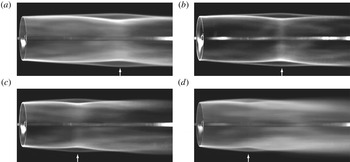
Dye patterns averaged over 22 rotor revolutions, for various tip speed ratios and
 $\unicode[STIX]{x1D6FF}/R_{0}=0.015$
: (a)
 $\unicode[STIX]{x1D706}=4.47$
, (b)
 $\unicode[STIX]{x1D706}=5.40$
, (c)
 $\unicode[STIX]{x1D706}=6.70$
, (d)
 $\unicode[STIX]{x1D706}=8.04$
. The white arrows indicate the positions of the leapfrogging.

For local pairing in the spatially evolving rotor wake, the leapfrogging also occurs, but only locally around the azimuth, e.g. at the top and bottom in figure 16. Subsequently, the wake structure becomes increasingly complex, and the concentrated vortices eventually get so entangled that they break down into small-scale turbulence. A similar behaviour was found for the late stages of local pairing in a single helical vortex (Quaranta et al. Reference Quaranta, Bolnot and Leweke2015).
The nonlinear late stages of global pairing evolve quite differently. Interestingly, after the leapfrogging, the wake almost recovers its initial double-helix structure, for which then a new leapfrogging event can build up again through global pairing. Selçuk et al. (Reference Selçuk, Delbende and Rossi2018) have numerically observed repeated leapfrogging of two helical vortices, with the number of cycles (before merging) depending on the helix pitch and the Reynolds number.
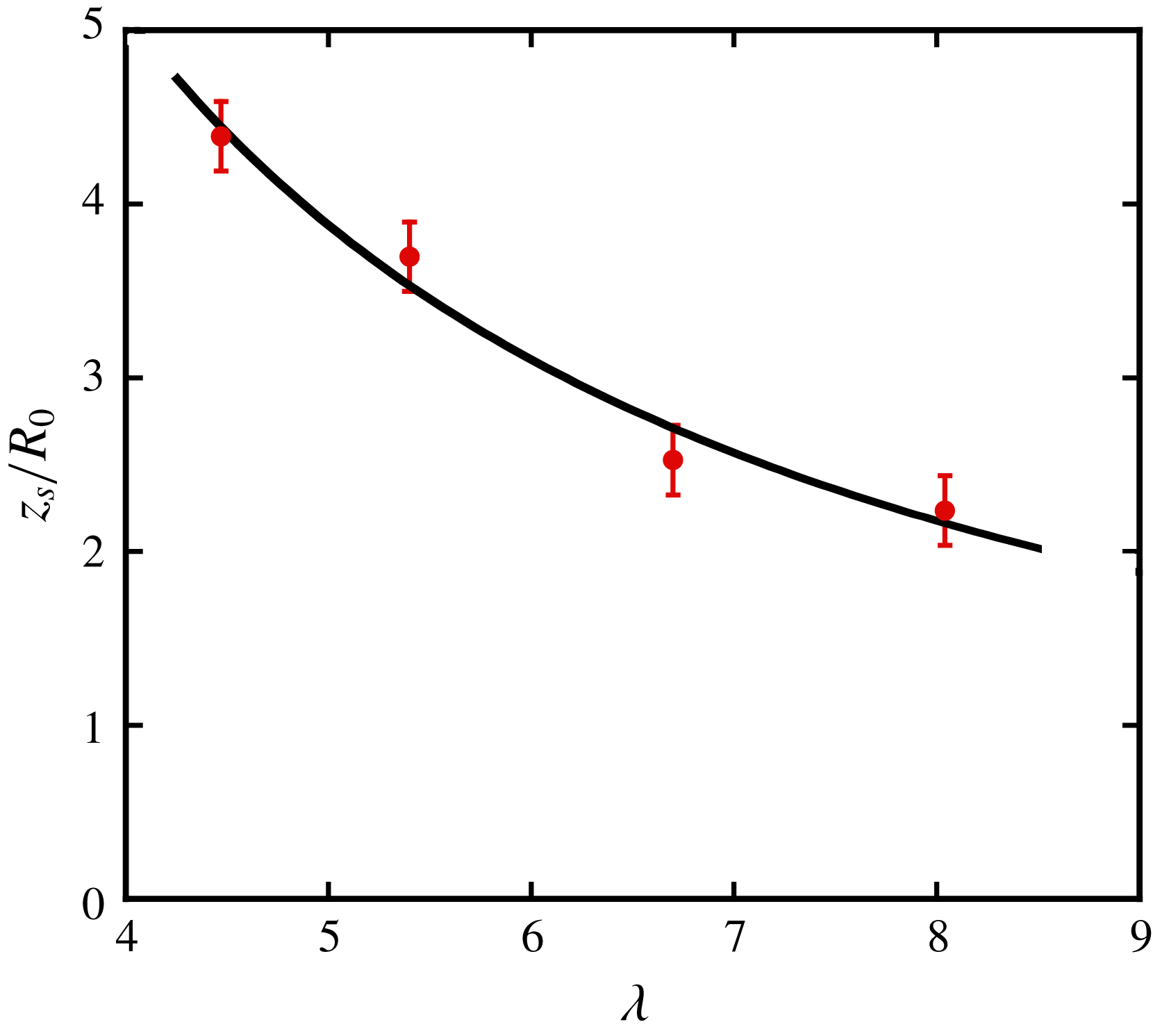
The leapfrogging (or vortex swapping) location can be found visually with some precision by considering time-averaged dye visualisations of the blade-tip vortices. Figure 24 shows examples of such averaged dye patterns, obtained for the four different tip speed ratios, with the swapping locations marked by arrows. It is found that this location moves upstream with increasing tip speed ratio. An increase of the tip speed ratio from
 $\unicode[STIX]{x1D706}=4.47$
to
 $\unicode[STIX]{x1D706}=8.04$
decreases the extent of the linear wake region by almost 50 %. Following the modelling by Sarmast et al. (Reference Sarmast, Dadfar, Mikkelsen, Schlatter, Ivanell, Sørensen and Henningson2014) of the linear phase of the pairing instability behind a rotor, the displacement amplitude (e.g.
 $d_{1}$
in figure 17
b) can be expressed as a function of downstream distance:
 $d_{1}(z)=d_{0}\exp (c_{1}^{-1}\unicode[STIX]{x1D706}z/R_{0})$
, where
 $d_{0}$
is the initial amplitude at
 $z=0$
and the parameter
 $c_{1}$
depends on the rotor properties. Assuming that, at the swapping location
 $z_{s}$
, the perturbation amplitude is always given by the same fraction of
 $h$
, and that
 $h$
is inversely proportional to the tip speed ratio (Sarmast et al.
Reference Sarmast, Dadfar, Mikkelsen, Schlatter, Ivanell, Sørensen and Henningson2014), one has
 $d_{1}(z_{s})\propto \unicode[STIX]{x1D706}^{-1}$
, which leads to
 $$\begin{eqnarray}\frac{z_{s}}{R_{0}}=\frac{c_{1}}{\unicode[STIX]{x1D706}}(c_{2}-\ln \unicode[STIX]{x1D706}).\end{eqnarray}$$
When the rotor properties do not vary, and the initial amplitude
 $d_{0}$
is the same (as for the series in figure 24),
 $c_{1}$
and
 $c_{2}$
are constants. In figure 25, this prediction is compared to the experimental measurements, and the agreement is found to be quite good.
Leapfrogging distance
 $z_{s}$
of neighbouring helix loops, as a function of the tip speed ratio
 $\unicode[STIX]{x1D706}$
. The solid line is a least-squares fit of (6.1).

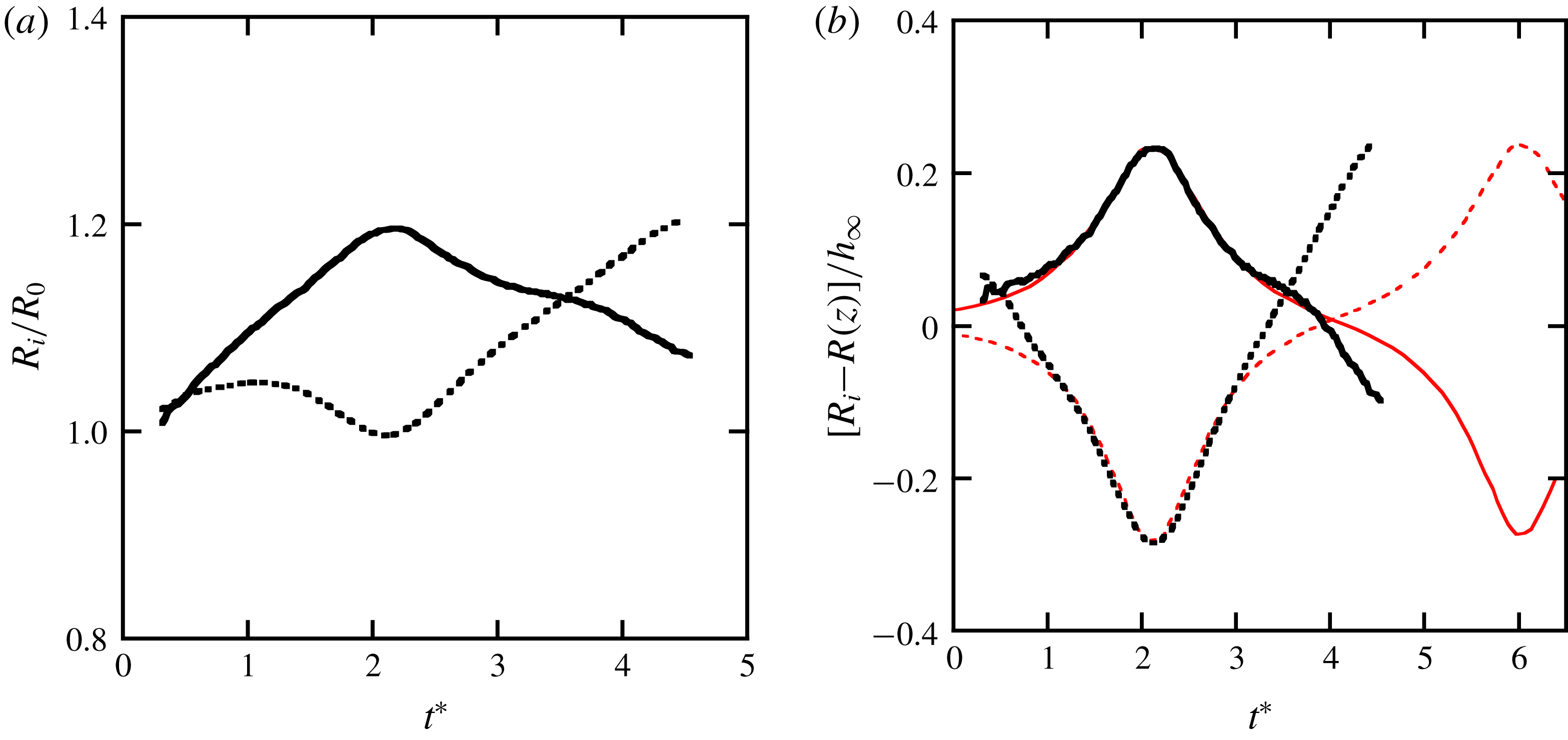
(a) Temporal evolution of the radii
 $R_{i}$
(
 $i=1,2$
) of two consecutive vortex loops for
 $\unicode[STIX]{x1D706}=6.70$
(
 $h_{\infty }/R_{0}=0.384$
,
 $a/R_{0}=0.034$
,
 $Re=4720$
), showing a complete cycle of leapfrogging and the onset of a second cycle. (b) Rescaled values, using the local radius
 $R(z)$
of the unperturbed helices (figure 14
a) and
 $h_{\infty }$
, and comparison with the numerical result (thin red lines) for two infinite helices with
 $h/R=0.943$
,
 $a/R=0.060$
and
 $Re=10\,000$
(Selçuk et al.
Reference Selçuk, Delbende and Rossi2018).

Multiple leapfrogging cycles could not be observed in our experiments, due to the limited length of the observation interval downstream of the rotor. Nevertheless, for the highest tip speed ratios (
 $\unicode[STIX]{x1D706}=6.67$
and 8.04), the onset of a second swapping could be detected, as shown in figure 26. When rescaled values are used (figure 26
b), a surprisingly good agreement is found with the numerical results from Selçuk et al. (Reference Selçuk, Delbende and Rossi2018) concerning the first swapping event, despite the differences in pitch, core size and Reynolds number, and the fact that one configuration is spatially evolving and the other one spatially uniform. This shows again that, for the pairing instability, the relevant scales of length (deformation amplitude) and time are indeed
 $h$
and
 $2h^{2}\unicode[STIX]{x1D6E4}$
, respectively, and that the core size and Reynolds number have little effect in the range of values considered here.
7 Summary and conclusions
In this study, the long-wave instability of a system of two interlaced helical vortices has been investigated. This configuration is of fundamental interest in the context of vortex dynamics and interactions, and it is also related to various applications involving the flow behind rotors. Examples are wind turbine or helicopter wakes, where instability phenomena of the vortex system can potentially have a significant impact.
The displacement instability of multiple helical vortices had previously been treated theoretically by Gupta & Loewy (Reference Gupta and Loewy1974), who extended the analysis of a single helical vortex by Widnall (Reference Widnall1972). In the first part of the present work, we revisit these earlier results and apply them to the two-helix flow subsequently studied experimentally. The system is unstable with respect to periodic displacement perturbations, the most unstable being those where the shift of neighbouring filaments (in the direction of the helix centreline) is out of phase, leading to local pairing of the vortices. This can occur when the perturbations on both vortices are, at the same axial position, either in phase or out of phase. The growth-rate curve, as a function of the perturbation wavenumber
 $k$
(number of wavelengths in one helix turn), consists of a sequence of lobes with maxima at integer values of
 $k$
. Contrary to the single-helix case studied in Quaranta et al. (Reference Quaranta, Bolnot and Leweke2015), two helices may also undergo a global pairing for
 $k=0$
.
It is possible to establish a link between the long-wave instability of the two-helix system and the three-dimensional pairing instability of an array of straight parallel vortices. When transposing the theoretical results obtained by Robinson & Saffman (Reference Robinson and Saffman1982) for the latter system to the helical geometry, a remarkably accurate prediction for the growth rate is obtained, demonstrating again that pairing of neighbouring filaments is the mechanism behind the long-wave instability of helical vortices with moderate pitch.
In the second part of this work, an experimental study is carried out, aimed at observing and characterising the various modes of the displacement instability in a real flow. Experiments are performed in a water channel, where a two-bladed rotor operating in the wind-turbine regime is used to generate the helical vortices. Carefully controlled experimental conditions allow the observation of an unperturbed two-helix system over a downstream distance of several rotor diameters, despite the highly unstable nature of the flow. The characteristics of this base flow, i.e. the overall helix geometry and the vortex velocity profiles (which reveal a significant velocity defect on the vortex axis), are obtained from dye visualisations and PIV measurements. Individual perturbation modes can then be triggered specifically and their structure and growth measured in detail. In-phase perturbations with non-zero wavenumber, leading to local pairing, are obtained by an appropriate modulation of the rotor rotation frequency, whereas out-of-phase perturbations with zero wavenumber, resulting in global pairing, are imposed by a radial offset of the rotor. For both cases, the mode shapes and the growth rates obtained through the post-processing of visualisation sequences are in good agreement with the corresponding theoretical predictions.
Experimentally, the phase of linear growth of the instability lasts until the maximum displacement has reached a value where neighbouring filaments are located at the same axial (downstream) position. For local pairing (
 $k\neq 0$
), the subsequent nonlinear evolution leads to strong deformations and a complex three-dimensional structure of the helical system, and eventually to a breakup of the concentrated vortices. This is similar to what is found for a single helical vortex (Quaranta et al.
Reference Quaranta, Bolnot and Leweke2015). The late stages of uniform pairing (
 $k=0$
) involve a global swapping (leapfrogging) of the two helices, which is here observed and characterised for various rotor-tip speed ratios. A quantitative comparison with results from the recent numerical simulations by Selçuk et al. (Reference Selçuk, Delbende and Rossi2018) concerning the time evolution of the helix radius confirms that the helix pitch is the relevant parameter for the scaling of the displacement amplitude and (together with the circulation) for time and the growth rate.
The theoretical analysis and the specifically designed experiments presented in this paper lead to a comprehensive assessment of the various unstable modes related to the long-wave pairing instability of two interlaced helical vortices, since not only the theory, but also the experimental procedure, can select the modes individually. In more general situations, such as full-scale applications involving rotor wakes, many of these modes may be triggered and grow simultaneously and interact – see, for example, the simulations of a three-bladed wind turbine wake by Sarmast et al. (Reference Sarmast, Dadfar, Mikkelsen, Schlatter, Ivanell, Sørensen and Henningson2014). In this situation, new phenomena may arise involving transient growth of certain mode combinations. This, and the related question of optimal perturbations leading to maximum amplitudes in a given finite time interval, will be explored in future work.
Acknowledgements
This work was supported by the Excellence Initiative of Aix-Marseille University – A*MIDEX, a French Investissements d’Avenir programme, in the framework of the Labex MEC; by the French Agence Nationale de la Recherche, project HELIX (ANR-12-BS09-0023-01); and by VR – The Swedish Research Council.