1. Introduction
Between 2019 and 2021 the number of undernourished people increased by approximately 126 million worldwide, prompting the heads of a group of international organizations including the Food and Agriculture Organization and the International Monetary Fund to declare the onset of a new global food security crisis (FAO et al. 2022).Footnote 1 The increase in the prevalence of undernourishment (PoU), a food security indicator that measures the share of the population whose dietary energy intake is below a minimum caloric threshold, was especially sharp during the pandemic-induced global recession of 2020. That year saw global real GDP contract by 2.9%, the steepest decline since the Great Depression. When the worst of the 2020 recession was over, however, food inflation then surged on account of supply chain disruptions and Russia’s invasion of Ukraine. Despite a global average increase of 19% in domestic food prices during 2021 and 2022, the global PoU stabilized in 2022. This coincided with a cumulative 10% increase in real world GDP over the same period. Notwithstanding cross-country differences in food inflation and recovery in economic activity, these events suggest that in recent years income fluctuations exerted a bigger impact on food insecurity than food inflation.Footnote 2 Footnote 3
Against this background, this paper sets out to quantify the impact of fluctuations in real income growth and food inflation on food insecurity, as measured by the PoU and two measures of diet composition (e.g., grams of animal protein per capita per day). To this end we utilize both a novel theoretical model and panel data with instrumental variables. Our main finding is that the positive effects of income growth in reducing the PoU are somewhat stronger than the negative effects posed by food inflation. As we highlight in the paper’s conclusion, we believe these findings are of interest for policymakers seeking to tackle food insecurity in the most efficient and effective manner.
To help organize our thinking regarding the macroeconomic determinants of food insecurity, we present a stylized heterogeneous-agent model. Households posses isoelastic non-homothetic CES preferences à la Matsuyama (Reference Matsuyama2019) over food and non-food, and vary in terms of their level of income. Food insecurity is defined as the fraction of households (at the lower end of the income distribution) who fall below an exogenous threshold in terms of food consumption. We also differentiate between an urban and rural economy variant of our model. In the rural variant, an increase in food prices leads to a windfall gain for farmers, directly increasing household income. Calibrating our model to the data for different regions in the world, the model delivers testable qualitative and quantitative predictions about the semi-elasticities of food insecurity with respect to income per capita and food prices.
The model is simple enough to show in a transparent way that the responsiveness of food insecurity to food price changes, for example, hinges on three critical factors: (i) the shape of the income distribution, (ii) the magnitude of the substitution elasticity relative to the income elasticity of food demand, and (iii) the degree of income redistribution. At the same time, the model is just complex enough to generate some unexpected predictions. Specifically, our calibrated model shows that higher food prices increase food insecurity, albeit modestly, in rural settings, as the income elasticity of food demand almost perfectly offsets the substitution elasticity—a finding that aligns with our empirical evidence as well as the existing literature.Footnote 4
Turning to the quantitative predictions, the calibrated model puts the global average income semi-elasticity of the PoU at approximately −0.12% points (pp). Stated differently, a doubling of income per capita should lead to a sizeable potential reduction of the PoU by 12 pp. Regarding the effect of food prices on the PoU, our model predicts that the semi-elasticity will be positive yet close to 0 in rural areas and around 0.12 pp in urban areas. Thus, when analyzing country-level PoU data, we would expect to find the food price elasticity to lie within these two bounds.
To empirically test the predictions of our model, we use a novel longitudinal dataset covering 142 countries for a period of two decades (2001–2021). We construct and collect from the literature several instrumental variables, namely (i) changes in a country’s commodity terms-of-trade, (ii) economic growth in trading partners, and (iii) external cereal harvest shocks, to isolate exogenous variation in domestic income growth and food inflation so that we can estimate their causal impact on food insecurity.
Our main findings are as follows. A 1 percentage point increase in economic growth leads to an approximately 0.11 pp reduction in the share of undernourished (0.79%), close to the prediction of our calibrated model.Footnote 5 In line with our model’s qualitative predictions, food inflation plays a more modest role, compared to real GDP growth, as the corresponding undernourishment elasticity, estimated at -0.06 pp (0.46%), is about 40% smaller. Finally, although countries that start out with higher levels of undernourishment show higher rates of reduction, the pace is slow, providing modest evidence of cross-country convergence in undernourishment.
Contributions and literature
Most research on food insecurity focuses on its sociodemographic determinants at the micro level (Borjas, Reference Borjas2004; Gundersen et al. Reference Gundersen, Pepper and Kreider2011). Our study contributes to a handful of papers that analyze the effects of aggregate economic factors on food insecurity (Headey, Reference Headey2013; Gregory and Coleman-Jensen, Reference Gregory and Coleman-Jensen2013).
The paper makes two contributions to the literature on food insecurity and inclusive growth more generally. First, to the best of our knowledge we are the first to present a tractable heterogeneous agent model of the macro drivers of food insecurity that generates testable predictions. Second, we simultaneously estimate the effects of income growth and food inflation on changes in food insecurity, allowing us to rank them in terms of quantitative importance, using an empirical strategy that explicitly addresses endogeneity concerns.Footnote 6 This is relevant because there is potential for reverse causality even in the short run, as can be the case when governments react to a deterioration in food security by increasing social protection spending or influencing food prices through monetary policy or direct control, which in turn may affect next year’s growth. Ignoring these issues leads to estimates biased towards zero, especially for the income elasticity of undernourishment.
The cross-country studies from Headey (Reference Headey2013), Soriano and Garrido (Reference Soriano and Garrido2016) and Headey and Hirvonen (Reference Headey and Hirvonen2023) are closest to our thematic focus. Soriano and Garrido (Reference Soriano and Garrido2016) find a 0.29% reduction in the share of food insecure for every 1 pp increase in real GDP per capita growth, in line with our OLS estimates but almost three times smaller than our preferred IV approach, which corrects for possible endogeneity and is also much closer to the magnitudes predicted by our theoretical model.Footnote 7 Headey (Reference Headey2013) finds that higher food prices exacerbate food insecurity. His measure of food insecurity is a subjective micro-level one, however, which makes his estimates not directly comparable to ours, since we use objective aggregate indicators of food insecurity. The latter are non perception-based and may offer more scope for cross-country comparability. Headey and Hirvonen (Reference Headey and Hirvonen2023) show that increases in annual real food prices predict reductions in poverty, but not in non-agrarian or more urban countries. Our model, which distinguishes between rural and urban settings and incorporates nonhomothetic preferences, provides a theoretical explanation for these empirical findings: higher food prices unambiguously increase food insecurity in urban areas while potentially reducing it in rural settings. Evidence for the farmer-income mechanism of higher food prices is presented by Dhingra and Tenreyro (Reference Dhingra and Tenreyro2021).
There are several secondary contributions to the literature worth noting. First, we study both quantitative and qualitative aspects of food insecurity to capture the connection between quantitative sufficiency and qualitative adequacy of diets.Footnote 8 The branch of the literature dealing with the latter has been dominated by micro studies looking into dietary changes in response to economic shocks (D’Souza and Jolliffe, Reference D’Souza and Jolliffe2014). Second, we are also the first to consider the role of social protection as a fiscal policy instrument to tackle food insecurity, while previous research had focused on how access to specific social protection programs (e.g., cash/food transfers) affects household food insecurity (Tiwari et al. Reference Tiwari, Daidone, Ruvalcaba, Prifti, Handa, Davis, Niang, Pellerano, van Ufford and Seidenfeld2016).
2. Model
2.1. Model Ingredients
Three manifestations of food insecurity with increasing degrees of severity are: worry about food, inadequate diet quality, and insufficient calorie intake (Wilde, Reference Wilde2011). Economists have focused on the latter manifestations, which can be measured through objective indicators while the former is subjective as it depends on perceptions. When an individual is below the minimum calorie intake there is a severe disutility from the physical and psychological discomfort of hunger. The marginal utility of extra calories is therefore high for calorie-deprived individuals, leading them to acquire the cheapest available source of calories, typically cereals, roots and tubers. Once more favorable combinations of income and food prices lift individuals above subsistence calorie levels, the marginal utility of extra calories declines rapidly and they substitute away from staples, introducing better tasting and more expensive foods into their diets, like meat, fish and fruits.
Nonhomothetic preferences for food and non-food
For the third and most severe aspect of food insecurity we present a stylized partial equilibrium model of food insecurity. Households buy food and non-food to maximize utility from consumption. Those that fall below an exogenous food consumption level are classified food insecure. Since the model features only one type of food, we are abstracting from any diet composition channel that, in case of negative shocks, would slow down (but not reverse) households descent into food insecurity.Footnote
9
A mass one of households is indexed by
 $h$
on the continuum
 $h\in [0,1]$
. Each household has identical affine non-homothetic preferences,
 $U$
, over a food bundle,
 $C_F$
, and a non-food bundle of consumption,
 $C_{NF}$
, such that
 \begin{gather*} U= \begin{cases} v(C_F) & \operatorname{for } 0\lt C_F\lt \underline {C_F}\\ u (C_F-\underline {C}_F,C_{NF}) & \operatorname{for } C_F\ge \underline {C_F} \end{cases} \end{gather*}
where
 $\underline {C}_F\gt 0$
is the food subsistence requirement, or basic need threshold, such that
 $\sup _{C_F} v(c_F)\lt \inf _{C_F,C_{NF}} u(C_F,C_{NF})$
, with
 $C_F$
and
 $C_{NF}$
defined in their respective support intervals. This utility function captures the notion that households have lexicographic preferences until food consumption reaches a basic need level.
We follow a number of recent papers in the literature on structural change, including Matsuyama (Reference Matsuyama2019), Comin et al. (Reference Comin, Lashkari and Mestieri2021), and Nath (Reference Nath2023), by assuming that subsistence utility
 $U$
is implicitly defined through the following nonhomothetic utility function:
 \begin{equation} \left ( \alpha ^{\frac {1}{\eta }} U^{\frac {\epsilon _{F} - \eta }{\eta }} (C_{F} - \underline {C_{F}})^{1-\frac {1}{\eta }} + (1- \alpha )^{\frac {1}{\eta }} U^{\frac {\varepsilon _{NF} - \eta }{\eta }} C_{NF}^{1-\frac {1}{\eta }} \right )^{\frac {\eta }{\eta - 1}} \equiv 1\quad \operatorname{ for } C_F\ge \underline {C_F} \end{equation}
where
 $\eta \in (0,1) \cup (1,\infty )$
and
 $\epsilon _F\gt 0$
(
 $\epsilon _{NF}\gt 0$
) are parameters representing the constant elasticity of substitution and the income elasticity of food (non-food) respectively, and where we have extended the isoelastic nonhomothetic CES function by including a food subsistence requirement. The latter adjustment has been made to ensure that under certain parameter restrictions (i.e.
 $\epsilon _{NF}=\epsilon _F=1$
) equation (1) reduces to Stone-Geary CES, until recently the most popular choice for modeling nonhomothetic preferences.
Each household earns an income
 $y(h)$
, with households ranked on the continuum in ascending order such that
 $y(h^{\prime })\gt y(h^{\prime \prime }) \Leftrightarrow h^{\prime }\gt h^{\prime \prime }$
. Gross disposable income is
 $y^d(h) = y(h) + \tau (h)$
where
 $\tau :[0,1]\rightarrow \mathbb{R}$
is a redistributive tax scheme such that
 $\int _0^1 \tau (h)dh=0$
. Let
 $\mu _y$
denote average per capita income. Then social protection expenditures collected by (or taxes paid by) household
 $h$
are determined as follows
 $\tau (h)=-\kappa (y(h)- \mu _y)$
such that
 \begin{align} y^d(h)=(1-\kappa )y(h)+\kappa \mu _y. \end{align}
The variable
 $\kappa \in [0,1]$
controls the degree of redistribution and determines minimum income as a fraction of per capita income,
 $\kappa \mu _y$
. The size of the redistribution is thus proportional to
 $\kappa$
and to income dispersion. If
 $\kappa =0$
or
 $y(h)=\mu _y$
for all
 $h$
then
 $y^d=y$
.
Each household is a price taker in the food market. Let
 $p_F$
and
 $p_{NF}$
be the price of food and nonfood respectively. Then households maximize equation (1) subject to the budget constraint,
 $p_F C_F + p_{NF} C_{NF}=y^d(h)-p_F \underline {C_F}$
, resulting in the following demand for food and non-food respectively:
 \begin{gather} C_F(h)= \begin{cases} \dfrac {y^d(h)}{p_F} & \operatorname{for } C_F \lt \underline {C_F} \\ \underline {C_F} + \underbrace {\alpha \left ( \frac {y^d(h)-p_F \underline {C_F}}{P}\right )^{\epsilon _{F}-1} \left ( \frac {p_F}{P} \right )^{1-\eta }}_{\equiv m_F} \left (\frac {y^d(h)-p_F \underline {C_F}}{p_F}\right ) & \operatorname{for } C_F\ge \underline {C_F}\\ \end{cases} \end{gather}
 \begin{gather} C_{NF}(h)= \begin{cases} 0 & \operatorname{for } C_F \lt \underline {C_F}\\ \underbrace {(1-\alpha ) \left ( \frac {y^d(h)-p_F \underline {C_F}}{P}\right )^{\epsilon _{NF}-1} \left (\frac {p_{NF}}{P} \right )^{1-\eta }}_{\equiv m_{NF}} \left (\frac {y^d(h)-p_F \underline {C_F}}{p_{NF}}\right ) & \operatorname{for } C_F\ge \underline {C_F} \\ \end{cases} \end{gather}
where
 $m_F$
and
 $m_{NF}$
constitute the budget shares for food and non-food respectively, and where the price index
 $P=P(p_F,p_{NF},y^d(h))$
, satisfying
 $U=\frac {y^d(h)-p_F \underline {C_F}}{P}$
, is implicitly given by
 \begin{equation} \left [ m_F + m_{NF} \right ]^{\frac {1}{1-\eta }} \equiv 1 \end{equation}
Defining food insecurity
A household is undernourished if its calorie intake falls below a certain minimum
 $\underline {Q}$
, that is,
 $C_F \leq \underline {Q}$
, where
 $\underline {Q}$
is potentially higher than the subsistence or basic need threshold, i.e.,
 $ \underline {C_F} = \lambda \underline {Q}$
with
 $\lambda \leq 1$
. Armed with this definition and making use of equations (3) and (2), we can then derive the following expression for the income level that coincides with the undernourishment threshold, that is,
 \begin{equation} y^{\operatorname{{PoU}}} = \frac {\tilde {\alpha } p_F \underline {Q} - \kappa \mu _y}{1-\kappa }, \end{equation}
where
 \begin{equation} \tilde {\alpha } \equiv \frac { \lambda \alpha ^{\frac {1}{\epsilon _F}} + \left ( (1-\lambda ) \underline {Q}^{1-\epsilon _F} \left ( \frac {p_F}{P} \right )^{\eta -\epsilon _F} \right )^{\frac {1}{\epsilon _F}} }{ \alpha ^{\frac {1}{\epsilon _F} } } \gt 0. \end{equation}
Note that
 $1 / \tilde {\alpha }$
is the share of nominal income that affords the household the minimum food basket
 $\underline {Q}$
. The right-hand side of equation (6) depends on
 $y^{\operatorname{{PoU}}}$
(via
 $P$
), and thus represents an implicit solution to
 $y^{\operatorname{{PoU}}}$
. In the standard CES case (
 $\epsilon _{NF}=\epsilon _F=1$
), however,
 $P$
no longer depends on income and thus (6) represents an explicit solution.
Closing the model: inequality in urban and rural economies
Let income per capita
 $y$
be a continuous random variable with probability density function (PDF)
 $f(y;\; \boldsymbol{\theta })$
, cumulative distribution function (CDF)
 $F(y;\; \boldsymbol{\theta })$
, where
 $\boldsymbol{\theta }$
is a set of (typically two of three) parameters. The mean and standard deviation of the distribution are denoted by
 $\mu _y$
and
 $\sigma _y$
respectively. The CDF can be inverted to obtain the income level of a household with income rank
 $h$
, that is,
 $y(h)=F^{-1}\left (h;\; \boldsymbol{\theta } \right )$
. This function can be used to derive the Lorenz Curve, i.e., fraction of total income earned by the bottom
 $x$
% of the population,
 \begin{equation} L(x;\; \boldsymbol{\theta })\equiv \frac {\int _0^x F^{-1}\left (h;\; \boldsymbol{\theta }\right ) \,\operatorname{d}h}{\int _0^1 F^{-1}\left (h;\; \boldsymbol{\theta } \right ) \,\operatorname{d}h}, \end{equation}
which subsequently feeds into the calculation of the Gini inequality coefficient:
 \begin{equation} G(\boldsymbol{\theta })=1-2\left ( \int _0^{1} L(x;\; \boldsymbol{\theta }) dx\right ). \end{equation}
The share of the population that is undernourished is the fraction of households whose income is below the threshold income level
 $y^{\operatorname{{PoU}}}$
:
 \begin{equation} \operatorname{{PoU}} = F\left (y^{\operatorname{{PoU}}};\boldsymbol{\theta } \right ) \end{equation}
We consider CDF’s that satisfy the following conditions.
Assumption 1 (Growth is a rising tide that lifts all boats).There exists at least one parameter
 $\theta _i$
that maps into income per capita,
 $\mu _y=g(\theta _{i}, \boldsymbol{\theta _{-i}})$
with
 $\frac {\partial \mu _y}{\partial \theta _i}=\frac {\partial g }{ \partial \theta _i}$
and for which the following holds:
 $\frac {d F}{d \mu _y}=\frac {\partial F}{\partial \theta _i} / \frac {\partial \mu _y}{\partial \theta _i}\lt 0$
for all
 $y$
.
Assumption 2 (Growth preserves the income distribution).The CDF allows a closed form solution to the Gini coefficient,
 $G=G(\boldsymbol{\theta })$
, but is not affected by the growth parameter
 $\theta _i$
, i.e.,
 $\frac {\partial G}{\partial \theta _i}=0$
.
Assumption1 says that the probability distribution is controlled by at least one parameter that allows us to increase GDP per capita and shift the entire CDF to the right such that the fraction of undernourished people unambiguously declines (“trickle-down growth”). This thought-experiment will look somewhat different for each distribution: for the normal distribution mean GDP per capita is identical to the location parameter
 $\mu$
, i.e., so that
 $\frac {\partial \mu _y}{\partial \mu }=1$
and
 $\frac {\partial F}{\partial \mu _y}=\frac {\partial F}{\partial \mu }\lt 0$
; for the log-normal distribution the mean is also controlled by the location parameter
 $\mu$
(but not exclusively) with
 $\frac {\partial \mu _y}{\partial \mu }=\mu _y$
; and for yet other distributions such as the Pareto Type 1 CDF both a scale and shape parameter satisfy Assumption1.
Assumption2 says that the parameter used to induce GDP per capita growth should not affect the degree of Gini inequality. This ensures that the results from comparative statics on the relationship between income per capita growth and the PoU are not conflated by changes in the income distribution. This assumption of “neutral income growth” also narrows down the number of parameters that can be used to induce GDP per capita growth, as for some distributions more than one parameter may satisfy Assumption1.Footnote 10
In addition to their effects on the affordability of the food minimums (
 $\underline {Q}$
), higher food prices may also affect food insecurity by boosting income per capita through windfall gains for farmers. To incorporate such an income effect, let us differentiate in a stylized manner between urban and rural economies. In the urban economy, as before, households have a claim on national income, as captured by the income distribution function. We assume that food prices do not affect income in the urban economy. In the rural economy, instead, the income distribution is an agricultural endowment distribution, i.e., it represents the heterogeneous claims that households hold to aggregate agricultural output or the total land endowment. Here higher food prices will boost household nominal income in proportion to each households’ claim on the country’s agricultural output. Let
 $\unicode {x1D7D9}{(Rural)}$
be an indicator function that’s equal to one when the condition between brackets, i.e., the economy is rural, is satisfied, and zero when the economy is urban.
Finally, for matters of convenience to simplify the comparative statics for urban and rural economies we assume any CDF to be “homothetic,” a quality usually preserved for utility and production functions. We can formally summarize these assumptions:
Assumption 3 (Higher global food prices increase income only in rural economies).In rural economies, but not in urban economies, household nominal income constitutes a claim on the agricultural endowment, i.e.,
 $y(h)=p_F r_F(h)$
and
 $\mu _y = \int _{0}^{1} y(h) dh= p_F R_F$
where
 $R_F \equiv \int _0^1 r_F(h)dh$
, such that
 $\frac {d \mu _y}{d p_F} = \unicode {x1D7D9}{(Rural)} R_F$
.
Assumption 4 (Eligible CDFs are homogeneous of degree zero in in
 $y$
and
 $\mu _y$
.).CDFs must satisfy
 $F\left ( \lambda y;\; \lambda \mu _y \right ) = F( y;\; \mu _y )$
.For rural economies this implies:
 $\begin{align} \nonumber\\[-18pt]F\left (\frac {y}{p_F};\; R_F \right ) = F(y;\; p_F R_F ) = F(y;\; \mu _y) \\[-10pt]\nonumber\end{align} $
Two examples of CDFs satisfying Assumptions1, 2 and 4 are:
Example 1. The income (or agricultural endowment) CDF is log-normal:
 $F(y;\mu ,\sigma )=\Phi \left (\frac {\ln (y)-\mu }{\sigma }\right )=\Phi \left (\frac {\ln (\frac {y}{\mu _y})+ \sigma ^2 /2}{\sigma }\right )$
, where
 $\Phi (x)$
is the standard normal distribution, and Gini is given by
 $G=2\Phi \left (\frac {\sigma }{\sqrt {2}} \right )-1$
.
Example 2.
The income (or endowment) CDF is Pareto-like:
 $F(y;\mu ,\rho )=\left ( \frac {1}{1+\rho } \frac {y}{\mu } \right ) ^{1/\rho } = \left ( \frac {1}{1+\rho } \frac {y}{\mu _y} \right ) ^{1/\rho }$
.Gini is given by
 $G=\frac {\rho }{\rho +2}$
.
2.2. Comparative statics
Under Assumptions (1)–(4), we can then summarize the effects of changes in food prices and GDP per capita on the PoU in the following proposition.
Proposition 1 (Income, food prices, and the PoU. General case).Differentiating
 $\operatorname{{PoU}}$
with respect to
 $p_F$
,
 $\mu _y$
, and
 $\kappa$
, we can then state the following the results using semi-elasticities:
Footnote
11
 \begin{align*}{\quad\,\,\, \frac {\operatorname{d} \operatorname{{PoU}}}{\operatorname{d} p_F / p_F} =\left ( f\left (y^{\operatorname{PoU}}\right ) \underset { (\pm )}{\frac {\operatorname{d} y^{\operatorname{PoU}}}{\operatorname{d} p_F}} + \underset {(0/-)}{\frac {\partial F}{\partial \mu _y} \frac {\operatorname{d} \mu _y}{\operatorname{d} p_F}} \right ) p_F }\end{align*}
 \begin{align*}{\quad\,\, \frac {\operatorname{d} \operatorname{PoU}}{\operatorname{d} \mu _y / \mu _y} = \left ( \frac {\partial F}{\partial \mu _y} - f\left (y^{\operatorname{PoU}}\right ) \frac {\kappa }{1- \kappa } \right ) \mu _y \lt 0 }\end{align*}
 \begin{align*}{ \frac {\operatorname{d} \operatorname{PoU}}{\operatorname{d} \kappa / \kappa } = f\left (y^{\operatorname{PoU}}\right ) \left ( \frac { y^{\operatorname{PoU}} - \mu _y }{1-\kappa } \right ) \kappa \gtrless 0\quad \operatorname{ for } y^{\operatorname{PoU}} \gtrless \mu _y }\end{align*}
-
(i) Higher food prices change the nominal income level needed to buy the minimum calorie intake. This changes the PoU in proportion to the share of people
 $f\left (y^{\operatorname{PoU}}\right )$
that stand at the income threshold. In rural economies, the CDF also shifts to the right because higher food prices lead to windfall gains, subsequently raising GDP per capita. The overall effect of higher food prices is unclear.
-
(ii) Higher GDP per capita lowers the PoU by shifting the CDF to the right, and by increasing social benefits for households below average income.
-
(iii) an increase in the degree of income redistribution lowers the PoU provided income of the marginally food insecure household is below the mean.

Proof. Follows from Assumption (1)-(4) and inspection of the derivatives. See appendix.
Proposition1 examines how changes in food prices and GDP per capita affect food insecurity.Footnote
12
Our focus here is on the extensive margin of food insecurity, which considers the overall share of affected households (i.e., those below the threshold), rather than the intensive margin, which looks at thedegree of insecurity within households as measured by their food consumption level. Consequently, the change in the PoU in response to income and food price fluctuations is shaped not only by parameters of the demand function (as is true for the intensive margin of food insecurity), but also by attributes of the income distribution. For example, a marginal increase in food prices affects food consumption for all households to some degree, but how many households will actually slide below the threshold as a result depends on the fraction of people
 $f(y^{\operatorname{PoU}})$
that stand at said income floor.
Under quite general conditions, Proposition1 tells us that while economic growth and larger social transfers unambiguously serve to lower the PoU, the effects of higher food prices are unclear. In order to obtain sharper predictions (even regarding the sign of the price elasticity), one must assume specific functional forms and put further restrictions on model parameters.Footnote
13
Furthermore, particularly sharp qualitative predictions can be obtained when preferences are further restricted to CES (
 $\varepsilon _F=\varepsilon _{NF}=1$
).Footnote
14
For ease of exposition we also mute the redistribution channel (
 $\kappa =0$
):
Proposition 2 (Income, food prices, and the PoU. CES case.).Consider Example 2 with CES preferences. The closed-form solutions to the PoU in urban and rural economies are:
 \begin{align*}{ \operatorname{PoU}_U\ = \left ( \frac {1}{1+\rho } \frac {\tilde {\alpha } (p_F/P) \underline {Q} }{R} \right ) ^{1/\rho } = f_U( \underset {+}{p_F},\underset {-}{R}) }\end{align*}
 \begin{align*}{\operatorname{PoU}_R\ = \left ( \frac {1}{1+\rho } \frac { \tilde {\alpha } (p_F/P) \underline {Q}}{ (p_F/P) R_F} \right ) ^{1/\rho } = f_R( \underset {-/+}{p_F} ,\underset {-}{R_F)} }\end{align*}
-
(i) In the urban economy, the positive price elasticity of the PoU is equal to or strictly smaller than the negative income elasticity in terms of magnitude iff
$\eta \leq 1$
(i.e.,
$\frac {{PoU}}{\operatorname{d}p_F / p_F} \leq - \frac {\operatorname{d}{PoU}}{\operatorname{d}R/R} = \frac {1}{\rho } {PoU} \lt 0$
).
-
(ii) In contrast, in the rural economy the food price elasticity of the PoU is positive only for
$\eta \gt 1$
, negative for
$\eta \lt 1$
, and zero for
$\eta =0$
.The (agricultural) income elasticity of the PoU is identical to the income elasticity in the urban economy (i.e.,
$\frac {\operatorname{d}{PoU}}{\operatorname{d}R_F/R_F} = - \frac {1}{\rho } {PoU} \lt 0$
).


Proof. Follows from inspecting the derivatives of equations (15)–(16). See also the appendix.
The food price elasticity of the PoU is governed by at most three sub-effects: a positive price effect and an expenditure share effect (
 $\gtrless 0$
for
 $\eta \gtrless 1$
) driving the demand for food, and a negative income effect for farmers (which is only present in rural economies). In the urban economy the food price elasticity is strictly positive as the price effect always dominates the expenditure share effect (which is negative when food and non-food are strict complements). This explains part (i) of Proposition2. In the rural economy, however, the income effect and the price effect perfectly offset each other, such that the expenditure share effect fully determines the sign of the food price elasticity.Footnote
15
If food and non-food goods are complements (substitutes), the food price elasticity of the PoU is negative (positive). This explains part (ii). In the real world, which is probably a blend of the stylized urban and rural models, we can then postulate that the food price elasticity can be negative, positive, or close to zero.
In addition to the key testable implications laid out in Propositions2, the model makes predictions on how the semi elasticities of food prices and income per capita change with the level of per capita income and inequality:
Proposition 3 (Structural characteristics and the semi-elasticity of PoU to income.).Consider again Example 2 with CES preferences. The responsiveness of the PoU to income:
-
(i) can become greater or weaker at higher levels of income, i.e.,
$\frac {\operatorname{d}}{\operatorname{d}\mu _y} \left ( \frac {\operatorname{d}{PoU}}{\operatorname{d} \mu _y/ \mu _y} \right ) = \frac {\operatorname{d}{PoU}}{\operatorname{d}\mu _y} \left ( \frac {\operatorname{d}{PoU} /{PoU}}{\operatorname{d}\mu _y/\mu _y} + \frac {\kappa }{1-\kappa } \frac {\mu _y}{y^{{PoU}}} \right ) \gtrless 0 \Leftrightarrow \rho \kappa \lessgtr \frac {\tilde {\alpha } p_F \underline {Q}}{\mu _y}$
. -
(ii) can become greater or weaker in countries with a higher degree of income inequality, i.e.,
$ \frac {\operatorname{d}}{\operatorname{d} \rho } \left ( \frac {\operatorname{d}{PoU}} {\operatorname{d}\mu _y/ \mu _y} \right ) \gtrless 0 \Leftrightarrow {PoU} \gtrless e^{- \frac {2+\rho }{1+\rho }}$
.


Proof. See appendix.
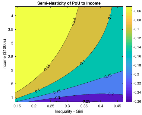
Consider how the income elasticity of the PoU changes when income increases. There are two effects. On the one hand, there will be fewer households to push out of undernourishment at higher levels of income and so the income semi-elasticity weakens. On the other hand, the absolute amount of income redistribution increases at higher income levels. Proposition3 (i) says that in theory the overall effect could go in either direction. Using parameter values representative of a low-income country, our model predicts that in practice the reaction of PoU to income growth tends to decline at higher levels of income (see Figure 1), which we empirically confirm in Section 6. Figure 1 also shows that the relation between the semi-elasticity and key parameters is highly non-linear.
The effect of inequality on the semi-elasticity of PoU to income is also ambiguous. There are two opposing effects. First, there is a direct effect that increases the impact of GDP growth on PoU because PoU increases with inequality (
 $\frac {d\operatorname{PoU}}{d\rho }\gt 0$
) and the income semi-elasticity increases in magnitude with PoU. The second effect works in the opposite direction: when inequality is high an increase in GDP growth is less “inclusive,” that is, in absolute terms it is less sizeable for poor households, thereby moving a smaller mass of households around the food security threshold. A simple, low-income country calibration exercise (see also the next section) predicts that the semi-elasticity of PoU to income is larger in magnitude in more unequal societies (see Figure 1), which implies that the first effect dominates.
3. Model calibration
We calibrate our model to match key macroeconomic data moments and targets. This calibration yields alternative estimates and bounds for income and price semi-elasticities of food insecurity, complementing our regression results. The calibration incorporates additional data not used in the regressions, including Gini coefficients, social protection spending, and external demand parameters.
3.1. Parameter estimates
Two simple calibration exercises are considered. In the first, we work with Stone-Geary Cobb-Douglas (CD) preferences (thus imposing
 $\epsilon _{F} = \epsilon _{NF} = \eta =1$
) and assume that income is Pareto distributed (i.e., this is our Example2). For our second calibration we stick with the Pareto income distribution, but on the consumer side we opt instead for isoelastic non-homothetic CES preferences.
Cobb-Douglas calibration
The parameter
 $\rho$
is set to match each region’s Gini coefficient by using the Gini equation for the Pareto distribution,
 $G=\frac {\rho }{\rho +2}$
. The household expenditure share on food,
 $\alpha$
, is based on that of a representative high-income country, i.e., Sweden, and comes from Haver Analytics. The parameter
 $\kappa$
is set equal to social protection expenditure as a share of GDP in 2010 based on data from the IMF and World Bank while
 $s_{q}$
is derived using GDP p.c. and our own estimate of the food component of the 2008 social poverty line figures (in 2011 PPP USD/day) for different income groups taken from Jolliffe and Prydz (Reference Jolliffe and Prydz2021). The parameter
 $\lambda$
is set such that, given all the before mentioned parameters, equation (15) matches each region’s 2010 PoU; and, finally, the semi elasticity then follows from substituting the estimated parameter values into the expression for
 $\frac {\operatorname{d} \operatorname{PoU}}{\operatorname{d} \mu _y / \mu _y}$
.
Isoelastic CES calibration
The following data points and parameters are identical to those of the Cobb-Douglas calibration: Gini, GDP p.c.,
 $\rho$
,
 $\kappa$
,
 $s_q$
, and
 $\operatorname{PoU}_0$
. Values for the parameters of the non-homothetic CES function are adopted from Nath (Reference Nath2023), that is,
 $\eta =0.27$
,
 $\epsilon _F=0.29$
, and
 $\epsilon _{NF}=1.08$
, where
 $\epsilon _{NF}$
is equated to the average income elasticity of the manufacturing and service sectors. Our estimate of the food budget share,
 $m_{NF}$
, is based on the suggestion by Smith and Subandoro (Reference Smith and Subandoro2007) that households who are most vulnerable to food insecurity spend in excess of 75% of their income on food. The parameter bundle
 $\tilde {\alpha }$
(and thus
 $\lambda$
) is then set such that equation (15) matches each region’s 2010 PoU; and, finally, the elasticities then follow from substituting the parameter estimates into equations (B20)–(B23) (see the appendix).
3.2. Predictions of price and income semi-elasticities
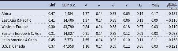
Starting with Stone-Geary CD preferences, a simple calibration of the model’s key parameters to different regions predicts a semi-elasticity of PoU to income (for both urban and rural economies) that ranges from −0.10 to −0.17% points (pp) and on average equals about −0.12 pp (see Table 1).Footnote 16 As the regression results in Section 6 show, our preferred estimate of the semi-elasticity of PoU to income is close to that prediction. When preferences are CD, Proposition2 tells us that for urban economies the food price elasticity is equal in magnitude to the income elasticity, but opposite in terms of sign. For rural economies, instead, the food price elasticity is zero (see Proposition2). This calibration thus indicates that the country-level food price semi-elasticity ranges from 0 to 0.17 pp, dependent on whether the rural or urban economy model better represents aggregate responsiveness of food insecurity to food prices.
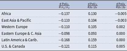
Next, consider our calibration with isoelastic non-homothetic preferences. As can be gleaned from Table 2, we find that the semi income elasticity of the PoU in this case is identical to the CD case. While the parameter bundle
 $\tilde {\alpha }$
depends on additional parameters in the case of isoelastic non-homothetic preferences compared to CD preferences, the calibration itself depends only on the aggregate value of the parameter bundle, not its individual components, and thus the income elasticities of the PoU are the same regardless of the type of consumer preferences. The price elasticities of the PoU, however, depend directly on the values of e.g., the consumer income elasticities for food and non-food. Ultimately, the price elasticities for the urban economies still end up being quite close to the opposite of the income semi-elasticity. This is because the sign and magnitude of the food price elasticity of the PoU are tightly linked to the ratio
 $\frac {\eta - \epsilon _{F}}{\epsilon _{F}}$
(see equations (B22)–(B23) in the supplementary appendix). Since the income elasticity of food
 $\epsilon _{F}$
and the substitution elasticity
 $\eta$
almost offset each other, that ratio ends up being close to zero just like the CD case (for which
 $\eta = \epsilon _F=1$
and thus
 $\frac {\eta - \epsilon _{F}}{\epsilon _{F}}=0$
). This is an important finding because a naive researcher, armed with merely a CES specification and a reasonable prior that food and non-food are complements (
 $\eta \lt 1, \epsilon _F=\epsilon _{NF}=1$
), would end up predicting that the food price elasticity of the PoU should be negative (which contrasts with our findings in Section 6). Finally, since
 $\frac {\eta - \epsilon _{F}}{\epsilon _{F}}$
is small, the food price elasticity for rural economies is also approximately equal to zero.
3.3. Summary
We have presented a heterogeneous agent model with non-homothetic preferences and used it to study the role of food prices and income per capita in driving food insecurity. The model rationalizes several empirical puzzles, including why food insecurity is less sensitive to food prices than to income per capita. The reason is that farmers receive windfall income gains from higher food prices that offset negative affordability effects. Related to this, the model also explains why in theory food price increases could actually reduce food insecurity (or poverty) in certain settings. While some of these puzzles have been addressed separately in other studies, our model constitutes a unified and analytically tractable framework to examine them together. Finally, two calibration exercises give a sense of the magnitude of the price and income elasticity that one could expect to see in the data. The semi-elasticity of PoU to income should range between −0.10 and −0.17 pp which implies that a doubling of income should lower the prevalence of undernourishment by 10–17 pp, a very sizeable effect. In contrast, when food prices fall by a 100% this leaves the PoU roughly unchanged in rural economies and lowers it by 9-16 pp in urban economies.
4. Data and descriptive statistics
From a measurement perspective, we focus on objective manifestations of food insecurity related to qualitative adequacy and quantitative sufficiency of diets (Wilde, Reference Wilde2011). To capture aspects of diet quality, we use the share of dietary energy from cereals, tubers and roots and the average supply of animal protein measured in grams per capita per day. For the most severe manifestation of food insecurity related to insufficient caloric intake we use the Prevalence of Undernourished (PoU). The PoU is defined as the share of a country’s population whose habitual food intake is insufficient to conduct an active and healthy life.
The PoU indicator as derived by FAO uses a log-normal probability density function for yearly dietary energy intake in the population, which requires the estimation of two parameters in order to fully characterize this distribution. The share of undernourished people in a country is then estimated as a cumulative probability of being below the minimum dietary energy requirements (MDER), i.e., the undernourishment threshold. More formally,
 \begin{equation} \operatorname{PoU}=\int _{x\lt \operatorname{MDER}} f(x|\Theta ) \,\operatorname{d}x \end{equation}
where
 $f(x|\Theta )$
is the log-normal distribution of caloric intake and
 $\Theta$
includes a location and a scale parameter. This function is intended to capture two dimensions of food security, namely food availability through the location (i.e., mean) parameter and differential food access through the higher moments (variance, skewness, and kurtosis). The mean is estimated every year from aggregate data on national food utilization accounts or from household survey data, when these are available. The other parameter and the MDER are estimated from micro data less frequently.
The literature has highlighted some limitations of the PoU, due to its top-down and aggregate approach. These limitations include the quality of the national food accounts data, the choice of a single undernourishment threshold for the whole country, and the lack of information on the severity of food insecurity. We refer the interested reader to FAO’s technical documentation for a detailed discussion (Cafiero, Reference Cafiero2014).
An alternative measure of food insecurity is the Food Insecurity Experience Scale (FIES), which overcomes the feasibility constraints faced by the PoU, as it does not require a costly dietary intake survey and the assumption of an undernourishment threshold. The main criticism against the FIES questions the comparability of perceived hunger experience across different individuals, countries and cultural contexts, while other authors highlight the possibility that it may overestimate food insecurity compared to insufficient-intake measures like the PoU (Barrett, Reference Barrett2010). We opt for the PoU as an objective and aggregate measure of national food insecurity, which has been selected by the United Nations to track progress towards the achievement of zero hunger by 2030. Further, the PoU has a much longer time coverage, spanning almost two decades, while the FIES is available only for three waves. This makes the PoU more suitable for our cross-country analysis on how food insecurity varies with business cycle fluctuations.
Data on GDP per capita and social protection expenditure come from the World Bank. We use real GDP per capita measured in constant 2015 dollars. Social protection expenditure in constant 2015 dollars includes current in-kind or cash transfers to households intended to provide for the needs that arise from social risks. They fall mostly under two broad categories: social security (e.g., unemployment benefits, retirement pension) and social assistance. Food inflation is defined as the year-on-year change in the food component of a country’s Consumer Price Index and is taken from the global inflation database constructed by Ha et al. (Reference Ha, Kose and Ohnsorge2023).
Our estimation sample comprises 142 countries across all continents and income groups and spans a period between 2001 and 2021. Countries with missing observations in a given year for the dependent or independent variables were dropped from the sample. We also drop observations if in a given year the country has experienced a high food inflation episode of above 50%, or a strong deflationary episode (bottom 10% of all observations). Our final estimation sample is an unbalanced panel.
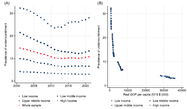
The left-hand side graph of Figure 2 shows the evolution of the PoU in the sample period by income group. Low-income countries show the most significant rates of undernourishment, with a 30% incidence compared to the global average of 10%. This gap with the rest of the world has widened in the recent decade.
The right-hand side graph of Figure 2 gives a descriptive view of the relationship between undernourishment and real GDP per capita. Undernourishment decreases with GDP per capita, but it also becomes less responsive to income growth as countries become richer.
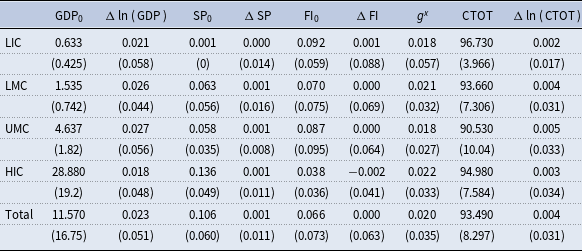
Table 3 describes the independent variables used in this study. GDP growth in the developing world has outpaced that in high-income countries. The level of food inflation in developing countries at the beginning of the observation period was almost double the one observed in the rich world (column 5), providing suggestive evidence of a positive association between food prices and undernourishment. The next column shows a secular reduction towards lower food inflation in upper-middle-income and high-income countries. Inflation is also least volatile in the group of high-income countries.
5. Empirical strategy
We are interested in estimating the relationship between aggregate food insecurity and its macroeconomic determinants. We can cast this relationship through a linear model:
 \begin{equation} y_{it}=\alpha +(\beta _0+\gamma _i)t+ \beta _1X_{it}+u_i+\epsilon _{it} {\\}, \end{equation}
where
 $y_{it}$
represents our measures of food insecurity for country
 $i$
at time
 $t$
, namely, the prevalence of undernourished, the share of dietary energy from cereals, roots and tubers, and animal protein supply. On the right-hand side of equation (18) the matrix
 $X_{it}$
includes our two main macro drivers, i.e., log real GDP per capita and food inflation (annual percentage change of the food component of the Consumer Price Index), as well as global and country time effects to control for phenomena that impact all countries in a similar fashion (
 $t$
). The composite error term includes country-specific time-invariant unobserved heterogeneity (
 $u_i$
) to capture geographical, historical or slow-changing institutional factors and a mean zero idiosyncratic shock (
 $\epsilon _{it}$
).
We adopt a first difference instrumental variables (FD-IV) estimation approach, to address concerns over omitted variables and reverse causality–which could lead to biased estimates from endogenous co-variation between the composite error term and the controls. In our setting, time-invariant unobservables (
 $u_i$
) may be correlated not only with food insecurity but also with the GDP and other right-hand side variables, potentially confounding the relationship. Taking the first difference of equation (18) eliminates
 $u_i$
, excluding the possibility of bias from correlation of
 $X_{it}$
with time-invariant confounders. This also allows to cast the relationship in terms of rates of change, since we are mostly interested in the short-term variations of food insecurity along the phases of the business cycle. It removes possible unit roots in the variables, making sure we are using stationary variables on both sides of the equation to avoid spurious findings. Finally, we utilize changes in food inflation rather than levels to net out the influence from monetary factors:Footnote
17
 \begin{equation} \Delta y_{it}=\beta _0+\theta y_{i0}+\beta _1 \Delta X_{it}+\Delta \epsilon _{it} , \end{equation}
where we assumed that
 $\gamma _i=\theta y_{i0}$
to capture a time-invariant regressor that controls for initial conditions allowing us to investigate whether there is convergence among countries towards some “equilibrium level” of food insecurity.Footnote
18
Countries that start out from higher levels of food insecurity should exhibit a faster pace of catching up.
Endogeneity may also stem from correlation of the controls with the idiosyncratic shock even after having netted out
 $u_i$
. This situation is often pervasive in a macro setting and potentially more problematic. For example, a given year’s shock to food security may feed back into next year’s fiscal budget as governments react quickly to distress situations by scaling up social protection spending, which in turn affects growth and prices (reverse causation). As a result, we may end up capturing a smaller (i.e. closer to zero) reaction of food insecurity to GDP growth than we would have in absence of this feedback effect. A similar result would be obtained for the coefficient of food inflation if governments reacted by introducing price controls for food items. All these scenarios invalidate the strict exogeneity assumption, which requires the error term to be uncorrelated with past, current and future values of the covariates (
 $E[\Delta \epsilon _{it}|X_{is}]=0$
for
 $s=1,2..t..T$
). The resulting least squares estimates of equation (19) would be biased towards zero.Footnote
19
We use external instruments for each endogenous variable to isolate plausibly exogenous variation. We instrument income growth with the average growth rate of a country’s trading partners and the change in the commodities terms of trade (Acemoglu et al. Reference Acemoglu, Johnson, Robinson and Yared2008; Burke, Reference Burke2012). In the average growth rate of trading partners the year-specific weights are given by the share in the previous three years of the country’s export to a given trading partner on total exports during the same period. For the second instrument of growth we use IMF’s commodity terms-of-trade (CTOT) index, which is the average of a range of commodity prices, each of which is weighed by the country’s share of net exports of a given commodity on its GDP over the previous three years (Gruss and Kebhaj, Reference Gruss and Kebhaj2021). (Details on the instruments are provided in the appendix).
Finally, food inflation is instrumented with a regional and a global (or “rest-of-world”) harvest shock. We use a Hodrick-Prescott filter to extract regional and global deviations from per capita trend production of (the calorie-weighted sum of) four grains - wheat, corn, soybeans, rice - which jointly provide more than two thirds of calories for human consumption, either directly or indirectly as livestock feedstuff. The regional supply shock for country
 $i$
represents the percentage deviation from per capita trend production across all countries within the region, except country
 $i$
. The rest-of-world shock for country
 $i$
represents the percentage deviation from total per capita trend production in all countries outside the country’s own region. To aggregate by region we follow the World Bank classification, which distinguishes between 7 regions: East Asia and Pacific, Europe and Central Asia, Latin America and Caribbean, Middle East and North Africa, North America, South Asia, and Sub-Saharan Africa (SSA). In the next section, we provide evidence of instrument relevance (
 $E[X_{it}|Z_{it}] \neq 0$
) and validity (
 $E[\Delta \epsilon _{it}|Z_{is}]=0$
for
 $s=1,2..t..T$
).
6. Results
This section presents the regression results for the PoU. Results for qualitative aspects of food insecurity (i.e., energy share of staples and protein consumption) are presented in an online supplementary appendix to conserve space. We focus on PoU in the main text as it is the primary indicator of food insecurity.
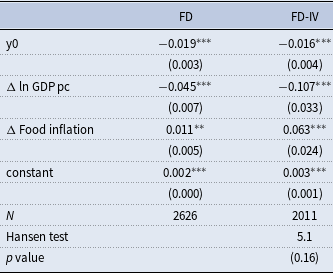
Table 4 shows the estimated coefficients for equation (19). The FD estimate of the marginal effect of income growth indicates that the PoU declines by roughly 0.05% points (pp) for every 1 pp increase in the GDP per capita growth rate, which, in relative terms, amounts to a 0.37% reduction (column 1).Footnote 20 This result is similar to Soriano and Garrido (Reference Soriano and Garrido2016), who find that a 1 pp increase in GDP per capita growth reduces PoU by 0.29%. When endogeneity is ignored, our results for income are similar to those found in previous articles that do not address the issue. Our OLS estimate of food inflation is also statistically significant and amounts to an increase of 0.011 pp in undernourishment, considerably smaller than the effect of income.Footnote 21 Headey (Reference Headey2013) finds that a measure of subjective food insecurity declines by 0.12–0.24 pp (0.47–1.25%) for a 1 pp increase in the real GDP per capita growth rate, while a 1 pp increase in relative food inflation increases undernourishment by 0.1–0.2 pp. Their work uses a different measure of food insecurity, which limits comparability to our results.
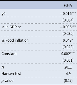
Instrumental variable estimates (column 2, Table 4) have the same signs as the OLS ones, but the magnitudes of all effects increase by at least a factor of 2. A 1 pp increase in income per capita growth leads to an approximately 0.11 pp reduction in the share of undernourished, which in relative terms translates into a 0.79% reduction. Food inflation also has a significant effect on undernourishment, but the effect is smaller than the effect of growth. For every 1 pp acceleration in food inflation, the share of undernourished increases by 0.06 pp (0.46%). We are unable to place this estimate in a range of plausible magnitudes since we are unaware of previous work on the effects of food inflation on the prevalence of undernourishment. In a typical year, with a sample standard deviation of 0.043 for GDP growth and 0.058 for inflation changes, a one standard deviation increase in GDP growth would lead to an estimated 3.4% reduction in undernourishment. In contrast, a one standard deviation increase in food inflation would result in an approximate 2.7% increase in the share of undernourished. The results on the sign of the effects of growth align with the model predictions summarized in Propositions1 and 2. We discus below the result on the sign and magnitude of the food inflation effect relative to that of income.
Finally, we find that countries that start out with higher levels of undernourishment at the beginning of our observation period exhibit, all things equal, a higher reduction rate. Starting out with a 1 pp higher PoU implies a faster reduction in PoU by 0.02 pp per year. This convergence effect is significant in both estimation approaches.
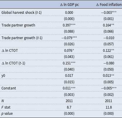
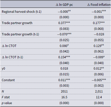
Standard diagnostic tests for the first and second stage show that our instruments are both strong predictors of the endogenous variables and uncorrelated with the error term. Results for the first stage (Table 5) show that our instruments have the expected sign and can induce variation in the endogenous variables. Current growth in trading partners is found to affect growth in the country of interest. Furthermore, improvements in the CTOT, stemming from increased (or decreased) prices of commodities that the country predominantly exports (or imports), positively affect short-term income growth. An F-test rejects the null hypothesis that the coefficients of the exclusion restrictions are jointly zero. For food inflation, we find that positive harvest shocks ease pressure on food prices, in line with our priors.
The validity of our instruments hinges on their independence from the error term in equation (19). The growth of a country’s trade partners and shifts in its terms of trade predominantly stem from external forces, minimizing the likelihood of feedback from domestic macroeconomic factors, let alone undernourishment. We posit that these instruments influence undernourishment solely via their impact on the nation’s GDP per capita growth and food inflation, rather than through hidden pathways that might contribute to the error term in our structural equation. This assertion gains strength when acknowledging that time-invariant or slow-moving variables such as institutional quality, which could correlate with the trading partners’ institutional capacity, have been netted out through first differencing.
As for harvest shocks, we argue that the trend in grains production reflects (slow moving) fundamentals of supply and demand. Deviations from this trend, identified using a Hodrick–Prescott filter, are likely indicative of external shocks outside of farmers’ controls, such as weather variability. The Hansen test statistics for instrument validity and the corresponding p values are reported in the last line of Table 4. We cannot reject the null hypothesis (p-value
 $\approx$
0.16) that our instruments are uncorrelated with unobserved drivers of food insecurity. These test results guarantee the consistency of the IV estimates.
Our results align with previous studies that use trade partners’ growth and commodity terms of trade changes as instruments for domestic growth, finding them to be both relevant and valid (Burke, Reference Burke2012). Finally, a Hausman test of endogeneity for
 $\Delta X$
based on the comparison of the FD vis-à-vis FD-IV sets of estimates did not provide sufficient evidence in favor of the null hypothesis that the potentially endogenous regressors can actually be treated as exogenous (p value 0). Considering this and the reliability of the instruments, FD-IV is our preferred set of estimates.
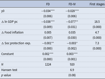
Further, we re-estimate equation (19) after adding the absolute change in social protection expenditure (% of GDP) as a control. This variable has a large number of missing values. Considering the big reduction in estimation sample size that this implies, FD and FD-IV results for this specification are shown separately in Table 6 and are not comparable to those of the baseline specification. FD estimates are in line with the model prediction, with social protection having a significant containing effect on undernourishment, although with a less steep gradient compared to that of income and food inflation.
The FD-IV estimates are based on the same set of instruments as before with the addition of age dependency ratio in the population as a dedicated instrument for social protection expenditure. The latter may drive social protection spending through its effect on the social security component (e.g. old age pensions). The FD-IV estimate of the social protection effect is considerably larger and still significant. While GDP growth and inflation have a similar scale, to be able to gauge the relative strength of social protection, we scale up its marginal effect by a factor of 4, which is the ratio of its standard deviation to that of the other two regressors. With this adjustment, a typical change in social protection expenditure leads to a reduction in undernourishment of 0.01 pp, considerably smaller than the inflation effect. However, the evidence on the effects of social protection is weak, at best, since first stage F statistics are lower and there is insufficient support for the validity of the instruments’ set.
6.1. Unpacking the effects of growth and inflation
We investigate heterogeneity of the short-term effects of food inflation and growth along selected structural characteristics of the economy by introducing interaction terms in our baseline specification:Footnote 22
 \begin{equation} \Delta y_{it}=\beta _0+ \theta y_{i0}+\beta _1 \Delta X_{it} +\beta _2W_{it} +\beta _3 \Delta X_{it}W_{it} +\Delta \epsilon _{it} , \end{equation}
where
 $W_{it}$
includes the mediating variables in levels. In one specification, we interact food inflation with the share of agricultural GDP, to investigate empirically the qualitative prediction of Proposition 2 of our theoretical framework. In an alternative specification, to provide empirical support to Proposition 4, we interact growth with GDP per capita which capture a country’s stage of economic development.
Equation (20) is estimated with the same FD-IV approach as equation (19). The inclusion of level variables poses a bigger threat to the exogeneity assumption, since in the long run a country’s level of income, for instance, is more likely to be both a determinant of undernourishment and diet composition and be affected by these variables in turn (Fogel, Reference Fogel2004). In this case, we resort to an alternative set of external instruments for the level variables
 $W_{it}$
, which is sourced from the literature and includes contemporaneous and one year lag of the average seasonal temperature levels and the old age dependency ratio in the population. These are added to the instruments for
 $\Delta X_{it}$
. The same set of instruments is employed whether
 $W_{it}$
comprises the share of agricultural GDP or metrics of GDP per capita.
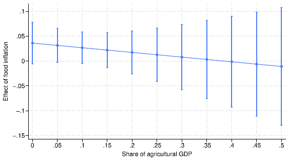
Our baseline findings showed that the impact of food inflation is positive and less pronounced compared to income growth. This could be attributed to the fact that while higher food prices unequivocally intensify food insecurity in urban economies, their effect may be quite small and potentially even negative in rural economies, because unlike urban residents rural populations may actually benefit from higher food prices in the form of an income effect due to their involvement in market-oriented agriculture (see Proposition2). To see if we could find support for this hypothesis, we explored whether the impact of food inflation on the PoU diminishes in proportion to the share of agricultural GDP. Figure 3 shows the FD-IV total effect of food inflation on undernourishment as a function of the share of agricultural GDP:
 $\beta _3(W)=\beta _1 + \beta _3 W$
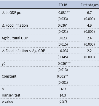
. The declining pattern provides some support for the model’s prediction, but it is only suggestive considering that the interaction term is statistically insignificant (Table 7).
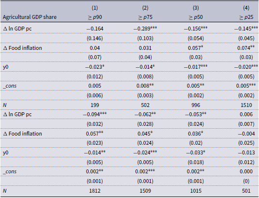
Power to detect significant interaction effects in a model is much smaller than for main effects, however, requiring a larger sample size. We therefore perform an alternative check based on subgroup analysis whose results are shown in Table 8.Footnote 23 The upper panel presents IV estimates of equation (19) for the sample with countries whose agricultural GDP share is above the 90th, 75th, 50th, and 25th percentiles (columns 1–4, respectively). The lower panel shows IV estimates for the complementary non-agricultural subsamples.
Expanding the agricultural sample with economies that are less agricultural, i.e., by moving rightwards across columns in the upper panel, we find that (i) the food inflation coefficient becomes larger and (ii) the gap between the income coefficient and the inflation coefficient becomes smaller. These findings are consistent with the farmer income mechanism that predicts that the effect of food inflation on the PoU is weaker (stronger) in more agricultural (urbanized) economies. In the lower panel, shrinking the urbanized sample by removing less urbanized i.e. more rural countries (moving rightwards), we see that the effect of both income and food inflation weakens. This is consistent with the idea that the impact of growth and food inflation on food insecurity (PoU) weakens in richer and more urbanized economies. This “high-income dilution” effect works in the opposite direction of the farmer income mechanism (see also Proposition3).
Furthermore, in columns 1 and 2 the food inflation coefficient is smaller in the agricultural sample (upper panel) than in the non-agricultural sample (lower panel), which is again consistent with the farmer income mechanism. However, this pattern disappears in columns 3 and 4. This reversal makes economic sense: in column 3 and 4 we expect the high-income dilution effect to be strongest and the farmer income mechanism to be weakest.
We conclude that the detrimental but smaller impact of food inflation compared to income growth can be explained in at least two ways. First, it suggests that the estimated effect of food inflation on aggregate food insecurity may constitute some average of the hypothesized larger urban effect and the smaller (or even negative) rural effect. Second, it may be indicative of other underlying microeconomic factors that limit farmers’ benefits from higher prices, including the extent to which farm producers tap into domestic and international trade and how the aggregate gains are distributed between farmers and intermediate traders. These aspects deserve further investigation and are left for future research.
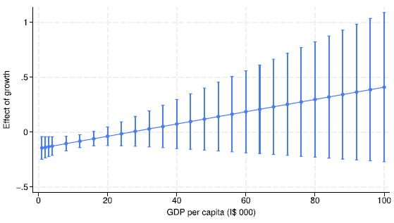
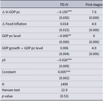
Further, the relationship between food insecurity and the GDP cycle can change over time as countries become richer or slowly adjust their structural characteristics. To see how the effects of growth vary with a country’s characteristics, in Figure 4 we plot the FD-IV total effect of growth against the GDP per capita level. Underlying estimates are shown in Table 9. First stage F tests reject the null hypothesis that the coefficients of the excluded instruments are jointly zero for all regressors. The Hansen test cannot reject the null hypothesis of exogeneity. Hence, we are confident about the overall consistency of the FD-IV estimates.
Figure 4 shows that undernourishment reacts to business cycle fluctuations for a broad range of income values (point-wise estimates are statistically significant through an income level of USD 20 thousand). Economic growth plays an important role in reducing hunger, especially at the early stages of development, but becomes less effective as countries grow richer and undernourishment plunges to low levels. This implies that the long term relationship between undernourishment and income is non-linear. This confirms the conclusions drawn from the descriptive analysis of Figure 2. For LICs that are still at the early stages of development undernourishment declines rapidly as income grows. For the HICs the curve is considerably less steep as income increases lead to smaller reductions in hunger. The higher income elasticity of hunger in middle- and low-income countries relates also to a larger share of the population that is closer to the undernourishment threshold and that is shifted above or below the threshold as income oscillates.
6.2. Sensitivity analysis
We conduct several robustness checks concerning the reliability of our instruments and the specification of the controls. To save on space, results of the robustness checks are provided only for the analysis of PoU.Footnote 24
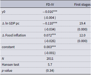
First, we check the sensitivity of our estimates to changes in the instruments set by replacing global harvest shocks with regional ones. Results for the second stage shown in Table 10 look very similar to those of our benchmark specification. The first stage estimates (Table 11) are also similar to the baseline specification with the regional shock having a smaller coefficient although still significant. Considering the ever integrated nature of grains markets, we would expect global shocks to have a greater influence on food inflation. We cannot reject the null hypothesis of instrument validity. In addition, we verified the robustness of our results by expanding the set of instruments with annual global temperature shocks from Bilal and Känzig (Reference Bilal and Känzig2024). Their research demonstrates that global temperature shocks are more significant predictors of domestic economic activity than local temperature fluctuations, primarily because global temperature variations correlate more strongly with extreme weather events like droughts. Consistent with Bilal and Känzig (Reference Bilal and Känzig2024), we find that global temperature shocks (and their first lag) serve as particularly strong instruments for income growth, thereby improving our first-stage F-statistics. However, our second-stage coefficients (Table 12) remain quantitatively similar to our benchmark specification.
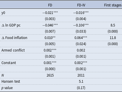
Second, the uptick in global food insecurity over the last decade is driven by low-income countries, particularly in SSA. One potential reason is a surge in armed conflicts (FAO, 2018; Andree et al. Reference Andree, Chamorro, Kraay, Spencer and Wang2020). To shed light on this hypothesis, we include a dummy variable that equals 1 if country
 $i$
was involved in an armed conflict in a given year. The dummy accounts for both conflicts occurring between two or more states as well as internal conflicts between the government of a state and one or more internal opposition groups. This variable comes from the Uppsala Conflict Data Program, while we use publicly available information to determine the territory on which fighting took place. Only conflicts with at least 1000 battle-related deaths in a given year are considered (see Davies et al. (Reference Davies, Pettersson and Öberg2022)).
Estimates of equation (19) with the armed conflict dummy are shown in table 13.Footnote 25 Only the FD estimate of the armed conflict effect is positive and statistically significant but not sizable (even accounting for scale, sd 0.35). After controlling for armed conflict, the effect of income growth and inflation are similar to the baseline estimates both for the FD and FD-IV model. For the latter, diagnostic tests indicate that the instruments are well correlated with the endogenous regressors and uncorrelated with the error term in the main equation. Thus, armed conflicts do not seem to have a direct effect on aggregate undernourishment and controlling for them leaves the coefficients of growth and inflation unchanged. However, previous research has shown that wars lead to a fall in output and a rise in inflation (Federle et al. Reference Federle, Meier, Muller, Mutschler and Schularick2024). Hence, we conclude armed conflicts might influence food security at the macro level only indirectly through income and food price channels.
7. Discussion
Following the Covid-19 pandemic and the global food price rally in the wake of Russia’s invasion of Ukraine, food insecurity has moved back to the top of the policy agenda of the international community.Footnote 26 While an in-depth reflection of how the international policy community and domestic policymakers reacted to the ongoing global food security crisis is beyond the scope of this paper, we observe that calls by international organizations to address the recent crisis have rested on a wide range of ideas, including (i) boosting agricultural production, (ii) a strengthening of safety nets for the most vulnerable, (iii) investing in climate resilient agriculture, and last but not least (iv) facilitating international free trade in food. All proposals are consistent with the importance of income growth in tackling food insecurity, even though they do not directly refer to (macroeconomic policies that can foster) inclusive economic growth. All proposals, except (ii), are linked directly to the idea that to lower food insecurity it is imperative to bring down food inflation.
Overall, this balance of policies seems mostly appropriate considering our empirical findings, but there is room for improvement. In our view, perhaps too much of the policy debate has revolved around fighting food inflation. We conjecture this is in part because policy makers typically rely on a mental model of food insecurity that is centered around purchasing power (for certain groups), i.e., the intensive margin of food insecurity. This mental model has appeal not only because urban middle class discontent about purchasing power played an important role throughout history as a catalyst for political change and conflict (e.g., during the Arab Spring), but also because policymakers often engage with the issue of higher food prices primarily from the perspective of consumers rather than that of farmers.Footnote 27 However, the UN Sustainable Development Goals are framed around the PoU, the metric used in this paper that measures the fraction of households whose calorie intake is insufficient. This metric compels policymakers to devise strategies that elevate the most vulnerable households above said threshold.
This paper has demonstrated that fostering economic growth is the most effective strategy for tackling food insecurity, closely followed by reining in food inflation. In light of this, policymakers should revise their understanding of the drivers of food insecurity and prioritize policies that promote inclusive growth by guaranteeing equal opportunities for everyone and those with disadvantaged backgrounds in particular and by implementing redistribution. They should also allow global food price increases to trickle down to domestic prices while enhancing targeted social protection within fiscal limits. This strategy would encourage sufficient food production, increase the incomes of food-insecure farmers, and protect the purchasing power of vulnerable urban households. It is important, however, to assess this strategy on a case-by-case basis, as some countries may have limited capacity to flexibly adjust their social protection systems to increase coverage or modify the size of transfers based on specific needs or episodes.
Acknowledgements
The authors would like to thank Petya Koeva Brooks, Gita Gopinath, Ishan Nath, and Tim Willems for their valuable suggestions, and Claire Li, Wenchuan Dong, and Joseph Moussa for their excellent research assistance. We have benefited from many discussions with and suggestions from participants of the IMF surveillance meeting, the April 2023 IMF Analytical Corner presentation, and the IMF Research Department Lightning Seminar. A very preliminary version of our paper was presented at the 2021 British Society for Population Studies Annual Conference at the London School of Economics. The data underlying this article will be shared on reasonable request to the corresponding author.
Competing interests
The authors declare that they did not receive external funding for this research and that there are no conflicts of interest.
Supplementary material
The supplementary material for this article can be found at http://doi.org/10.1017/S1365100525100369.
Appendix A: Tables and figures
The sensitivity of the semi-elasticity of PoU to income with respect to income and inequality. Figure drawn for
 $\eta =\epsilon _F=\epsilon _{NF}=1$
,
 $\alpha =0.14$
,
 $\underline {C_F}=0.5$
,
 $\kappa =0.05$
,
 $\lambda =0.97$
, and with
 $p_F$
chosen such that
 $s_q \equiv \frac {p_F \underline {Q}}{\mu _y}=0.14$
for
 $\mu _y=2.5$
.

Income (and food price) elasticity of the PoU. Cobb-Douglas preferences

Note: GDP p.c. (in constant 2015 USD) is the region average for 2010 and is taken from the World Bank ICP database; Gini is the region average 2010 Gini coefficient and is collected from Darvas (Reference Darvas2019);
 $\operatorname{PoU}_0$
is the region’s average 2010 PoU. Reported values of
 $\kappa$
,
 $s_q$
and
 $\operatorname{PoU}_0$
also represent region averages, i.e., unweighted averages across all countries within each region, subject to data availability. Parameter selection and estimation are described in the main text.
Income and food price elasticities of the PoU. Isoelastic non-homothetic CES preferences

Note: Except for the parameter values of the isoelastic CES function, which are adopted from Nath (Reference Nath2023), all data points and parameters used are identical to those of the CD calibration presented in Table 1. See explanation in the main text.
(A) evolution of PoU over time and by income group (B) relationship between undernourishment and GDP per capita by income group.

Descriptive statistics: controls and instruments

Note: Sample averages by income level of the initial value of real GDP per capita in thousands of 2015 $ (
 $\operatorname{GDP}_0$
), social protection expenditure as share of GDP $ (
 $\operatorname{SP}_0$
) and food inflation
 $\operatorname{FI}_0$
.
 $\Delta$
ln(GDP), is the growth rates of real income.
 $\Delta \operatorname{FI}$
and
 $\Delta$
SP are the absolute change of food inflation and social protection spending as a share of GDP.
 $g^{x}$
is trade partners’ growth. We use the World Bank definition of income groups. Standard errors are in parenthesis.
Estimation results of main equation: PoU

Note:
 $^{***}$
 $p\lt 0.01$
,
 $^{**}$
 $p\lt 0.05$
,
 $^{*}$
 $p\lt 0.1$
. Column 1 shows OLS results while column 2 has the corresponding IV estimates.
First stages of main equation: PoU

Note:
 $^{***}$
 $p\lt 0.01$
,
 $^{**}$
 $p\lt 0.05$
,
 $^{*}$
 $p\lt 0.1$
. Column 1 shows first stage estimates for GDP growth and column 2 for inflation changes.
Estimation results of main equation: extended controls (1)

Note:
 $^{***}$
 $p\lt 0.01$
,
 $^{**}$
 $p\lt 0.05$
,
 $^{*}$
 $p\lt 0.1$
. Column 1 shows OLS results while column 2 has the corresponding IV estimates. The last column shows the F test statistics from the first stage of each regressor and the corresponding p value.
Food price effects variation for undernourishment.

Food inflation effects heterogeneity: agricultual GDP

Note:
 $^{***}$
 $p\lt 0.01$
,
 $^{**}$
 $p\lt 0.05$
,
 $^{*}$
 $p\lt 0.1$
. The first column shows IV estimates of equation (20). The last column show the F test statistics from the first stage of each regressor and its p value.
Subsample estimates of inflation effects

Note:
 $^{***}$
 $p\lt 0.01$
,
 $^{**}$
 $p\lt 0.05$
,
 $^{*}$
 $p\lt 0.1$
. The upper panel presents IV estimates of equation (19) for countries with agricultural GDP share above the 90th, 75th, 50th, and 25th percentiles (columns 1–4, respectively). The lower panel shows IV estimates for the complementary non-agricultural subsamples corresponding to each column above. The observations in each column’s upper and lower panels sum to 2011, reflecting the complete sample split at different agricultural intensity thresholds.
Growth effects variation for undernourishment.

Interactions equation estimates: growth effects on PoU

Note:
 $^{***}$
 $p\lt 0.01$
,
 $^{**}$
 $p\lt 0.05$
,
 $^{*}$
 $p\lt 0.1$
. The first column shows IV estimates of equation (20). The last column shows the F test statistics from the first stage of each regressor and its p value.
Estimates with alternative set of instruments

Note:
 $^{***}$
 $p\lt 0.01$
,
 $^{**}$
 $p\lt 0.05$
,
 $^{*}$
 $p\lt 0.1$
.
First stage: alternative instruments

Note:
 $^{***}$
 $p\lt 0.01$
,
 $^{**}$
 $p\lt 0.05$
,
 $^{*}$
 $p\lt 0.1$
.
Estimation results of main equation: global temperature shocks as additional IV

Note:
 $^{***}$
 $p\lt 0.01$
,
 $^{**}$
 $p\lt 0.05$
,
 $^{*}$
 $p\lt 0.1$
. Column 1 shows IV results while column 2 shows the F test statistics from the first stage of each regressor and the corresponding p value.
Sensitivity to controlling for wars

Note:
 $^{***}$
 $p\lt 0.01$
,
 $^{**}$
 $p\lt 0.05$
,
 $^{*}$
 $p\lt 0.1$
. The last column shows the F test statistics from the first stage of each regressor and its p value.
Appendix B: Mathematical proofs
Proof of Proposition1 .
(i) We totally differentiate the system of equations (5)–(7) with respect to
 $p_F$
and
 $y^{\operatorname{PoU}}$
and then rearrange to obtain
 $\frac {\operatorname{d}y^{\operatorname{PoU}}}{\operatorname{d}p_F}$
, i.e., the food price derivative of the threshold income level associated with the PoU:
 \begin{equation} \begin{split} \frac {\operatorname{d}y^{\operatorname{PoU}}}{\operatorname{d}p_F} &= \frac { \left ( \tilde {\alpha } + p_F \frac {\operatorname{d} \tilde {\alpha }}{\operatorname{d} p_F} + p_F \frac {\operatorname{d} \tilde {\alpha }}{\operatorname{d}y^{\operatorname{PoU}}} \frac {\kappa }{1-\kappa } \frac {\operatorname{d}\mu _y}{\operatorname{d}p_F} \right )\underline {Q} - \kappa \frac {\operatorname{d} \mu _y}{\operatorname{d} p_F} }{ 1- \kappa - p_F \underline {Q} \frac {\operatorname{d} \tilde {\alpha }}{\operatorname{d}y^{\operatorname{PoU}}} } \\ &= \frac {\tilde {\alpha } \underline {Q}}{1-\kappa } \frac {1+\frac {\eta - \epsilon _F}{\epsilon _F} \frac {\tilde {\alpha } - \lambda }{\tilde {\alpha }} \left ( \xi _0 + \xi _1 \frac {p_F \underline {C_F} -y^{d \star } \kappa \frac {1}{ \tilde {\alpha } \underline {Q}} \frac {\operatorname{d}\mu _y}{\operatorname{d}p_F} }{y^{d \star } - p_F \underline {C_F}} \right ) - \frac {1}{\tilde {\alpha } \underline {Q}} \kappa \frac {\operatorname{d}\mu _y}{\operatorname{d}p_F} }{1 + \frac {\eta - \epsilon _F}{\epsilon _F} \frac {\tilde {\alpha } - \lambda }{\tilde {\alpha }} \xi _1 \frac { y^{d \star }}{y^{d \star } - p_F \underline {C_F}} } \end{split} \end{equation}
with
 \begin{align*}{\qquad \frac {\operatorname{d} \tilde {\alpha }}{\operatorname{d}y^{\operatorname{PoU}}} = - \frac { \eta - \epsilon _F}{\epsilon _F} ( \tilde {\alpha } - \lambda ) \frac {1}{P} \frac {\operatorname{d}P}{\operatorname{d}y^{\operatorname{PoU}}}, }\end{align*}
 \begin{align*}{ \frac {\operatorname{d} \tilde {\alpha }}{\operatorname{d} (p_F/P)} = \frac { \eta - \epsilon _F}{\epsilon _F} ( \tilde {\alpha } - \lambda ) \frac {1}{p_F/P} \gtrless 0\quad \operatorname{ if } \eta \gtrless \epsilon _F, }\end{align*}
 \begin{align*}{\qquad\quad\,\, \frac {\operatorname{d}P}{\operatorname{d}y^{\operatorname{PoU}}}= (1-\kappa ) \frac {P}{y^{d \star } - p_F \underline {C_F}} \xi _1 , }\end{align*}
 \begin{align*}{\qquad \frac {\operatorname{d} (p_F/P)}{\operatorname{d}p_F} = \frac {1}{P} \left (\xi _0 + \xi _1 \frac {p_F \underline {C_F}}{y^{d \star } -p_F \underline {C_F}} \right ), }\end{align*}
 \begin{align*}{\qquad\qquad \frac {\operatorname{d} \tilde {\alpha }}{\operatorname{d} p_F} = \frac {\operatorname{d} \tilde {\alpha }}{\operatorname{d} (p_F/P)} \frac {\operatorname{d} (p_F/P)}{\operatorname{d}p_F}, }\end{align*}
and where
 \begin{align*}{\qquad\qquad\quad y^{d \star } \equiv (1-\kappa ) y^{\operatorname{PoU}} + \kappa \mu _y }\end{align*}
 \begin{align*}{\qquad\,\,\, \xi _0 \equiv \left [ \frac { (\epsilon _F - 1) m_F + (\epsilon _{NF} - \eta ) m_{NF} }{ ( \epsilon _F - \eta ) m_F + (\epsilon _{NF} - \eta ) m_{NF} } \right ], }\end{align*}
 \begin{align*}{\qquad\,\,\, \xi _1 \equiv \left [ \frac { (\epsilon _F - 1) m_F + (\epsilon _{NF} - 1 ) m_{NF} }{ ( \epsilon _F - \eta ) m_F + (\epsilon _{NF} - \eta ) m_{NF} } \right ], }\end{align*}
 \begin{align*}{\qquad m_F \equiv \alpha \left ( \frac {y^d(h)-p_F \underline {C_F}}{P}\right )^{\epsilon _{F}-1} \left ( \frac {p_F}{P} \right )^{1-\eta } , }\end{align*}
 \begin{align*}{ m_{NF} \equiv (1-\alpha ) \left ( \frac {y^d(h)-p_F \underline {C_F}}{P}\right )^{\epsilon _{NF}-1} \left ( \frac {p_{NF}}{P} \right )^{1-\eta } , }\end{align*}
and
 $\frac {\operatorname{d} \mu _y}{\operatorname{d} p_F}$
is either 0 (urban economy) or
 $R_F$
(rural economy) (see Assumption3). Without further assumptions, one cannot sign the derivative
 $\frac {\operatorname{d}y^{\operatorname{PoU}}}{\operatorname{d}p_F}$
which can be positive or negative. That
 $\frac {\partial F}{\partial \mu _y} \frac {\operatorname{d} \mu _y}{\operatorname{d} p_F}$
is either zero or negative follows from the fact that
 $\frac {d \mu _y}{d p_F}$
is either zero (urban case) or positive (rural case), while
 $\frac {\partial F}{\partial \mu _y}$
is strictly negative based on Assumption1. This completes the proof for (i).
(ii)–(iii) The results follow directly from inspecting the expressions for the semi elasticities
 $\frac {\operatorname{d} \operatorname{PoU}}{\operatorname{d} \mu _y / \mu _y}$
and
 $\frac {\operatorname{d} \operatorname{PoU}}{\operatorname{d} \kappa / \kappa }$
and applying Assumption1.
Proof of Proposition2 .
(i)–(iv) The income and price semi-elasticities based on equations (15)–(16) read:
 \begin{equation*} \frac {\operatorname{d}\operatorname{PoU}_U}{\operatorname{d}R/R} = -\frac {1}{\rho } \operatorname{PoU} \lt 0 \end{equation*}
 \begin{equation*} \frac {\operatorname{d}\operatorname{PoU}_U}{\operatorname{d}p_F/p_F} = \frac {\tilde {\alpha } + (\eta -1) (\tilde {\alpha } - \lambda ) m_{NF} }{\tilde {\alpha } } \frac {1}{\rho } \operatorname{PoU}_U \gt 0 \end{equation*}
 \begin{equation*} \frac {\operatorname{d}\operatorname{PoU}_R}{\operatorname{d}R_F/R_F} = -\frac {1}{\rho } \operatorname{PoU} \lt 0 \end{equation*}
 \begin{equation*} \frac {\operatorname{d}\operatorname{PoU}_R}{\operatorname{d}p_F/p_F} = \frac { (\eta -1) (\tilde {\alpha } - \lambda ) m_{NF} }{\tilde {\alpha } } \frac {1}{\rho } \operatorname{PoU}_R \gtrless 0 \Longleftrightarrow \eta \gtrless 1 \end{equation*}
The results then follow from inspecting the signs of these semi elasticities (for
 $\eta \gtrless 1$
) and, where applicable, comparing the magnitudes of these derivatives. This completes the proof.
Proof of Proposition3 .
Let us define
 $s_q \equiv \frac {p_F \underline {Q}}{\mu _y}$
. Then note that the semi income elasticity in this case can be written as:
 \begin{equation} \frac {\operatorname{d}\operatorname{PoU}}{\operatorname{d}\mu _y/\mu _y} = - \frac {1}{\rho } \frac { \tilde {\alpha } s_q}{ \tilde {\alpha } s_q -\kappa } \operatorname{PoU} \lt 0 \end{equation}
Differentiating the semi income elasticity
 $\frac {\operatorname{d}\operatorname{PoU}}{\operatorname{d}\mu _y/\mu _y}$
with respect to
 $\mu _y$
and
 $\rho$
respectively, gives:
 \begin{equation} \begin{split} \frac {\operatorname{d}}{\operatorname{d}\mu _y} \left ( \frac {\operatorname{d}\operatorname{PoU}}{\operatorname{d}\mu _y/\mu _y} \right ) &= \frac {\operatorname{d}\operatorname{PoU}}{\operatorname{d} \mu _y} \left ( \frac {\operatorname{d}\operatorname{PoU} /\operatorname{PoU}}{\operatorname{d}\mu _y/\mu _y} + \frac {\kappa }{1-\kappa } \frac {\mu _y}{y^{\operatorname{PoU}}} \right ) \gtrless 0 \\ &\Leftrightarrow \frac {\kappa }{1-\kappa } \frac {\mu _y}{y^{\operatorname{PoU}}} \lessgtr - \frac {\operatorname{d}\operatorname{PoU} /\operatorname{PoU}}{\operatorname{d}\mu _y/\mu _y} = \frac {1}{\rho } \frac { \tilde {\alpha } s_q}{ \tilde {\alpha } s_q -\kappa } \\ &\Leftrightarrow \rho \kappa \lessgtr \tilde {\alpha } s_q \end{split} \end{equation}
and
 \begin{equation} \begin{split} \frac {\operatorname{d}}{\operatorname{d}\rho } \left ( \frac {\operatorname{d}\operatorname{PoU}}{\operatorname{d}\mu _y/\mu _y} \right )&= - \frac {1}{\rho } \frac {\operatorname{d}\operatorname{PoU}}{\operatorname{d}\mu _y/\mu _y} - \frac {1}{\rho } \frac {\tilde {\alpha } s_{q}}{ \tilde {\alpha } s_{q} - \kappa } \frac {\operatorname{d}\operatorname{PoU}}{\operatorname{d}\rho } \\ &= - \left ( \frac {\operatorname{d}\operatorname{PoU} / \operatorname{PoU}}{\operatorname{d}\mu _y/\mu _y} \right ) \left [ 1 + \frac {1}{1+\rho }+\ln \left ( \operatorname{PoU} \right ) \right ] \frac {\operatorname{PoU}}{\rho } \\ &= - \left ( \frac {\operatorname{d}\operatorname{PoU} / \operatorname{PoU}}{\operatorname{d}\mu _y/\mu _y} \right ) \left [ 1 + \ln \left ( \frac {\operatorname{PoU}}{\overline {\operatorname{PoU}}} \right ) \right ] \frac {\operatorname{PoU}}{\rho } \gtrless 0 \Leftrightarrow \operatorname{PoU} \gtrless e^{- \frac {2+\rho }{1+\rho }} \end{split} \end{equation}
where the last step in equation (33) follows from
 $\frac {\kappa }{1-\kappa } \frac {\mu _y}{y^{\operatorname{PoU}}} = \frac {\kappa }{\tilde {\alpha } s_q - \kappa }$
. This completes the proof.
Derivatives for model calibration with isoelastic non-homothetic CES preferences
Let
 $\phi (x) \equiv \frac {1}{\sigma \sqrt {2 \pi }} e^{-x^2/2}$
and
 $\Phi (x) \equiv \int _{-\infty }^{x} e^{-t^2/2}\operatorname{d}t$
represent the PDF and the CDF of the standard normal distribution. Then the lognormal CDF’s for the urban and rural economy respectively are:
 \begin{equation} F_U = \Phi \left ( \frac {\ln \left (y^{\operatorname{PoU}}\right ) - \mu } {\sigma }\right )=\Phi \left ( \frac {\ln \left (\frac {y^{\operatorname{PoU}}}{ \mu _y}\right ) + \sigma ^2 /2 } {\sigma }\right ) \end{equation}
and
 \begin{equation} \nonumber\\[-30pt]F_R = \Phi \left ( \frac {\ln \left (y_R^{\operatorname{PoU}}\right ) - \mu } {\sigma }\right ) = \Phi \left ( \frac {\ln \left (\frac {y_R^{\operatorname{PoU}}}{ \mu _y}\right ) + \sigma ^2 /2 } {\sigma }\right ) \end{equation}
where
 \begin{align*}{ \frac {y^{\operatorname{PoU}}}{ \mu _y} = \frac { \tilde {\alpha } p_F \underline {Q} -\kappa \mu _y}{ (1- \kappa ) \mu _y} }\end{align*}
 \begin{align*}{\,\,\, \frac {y_R^{\operatorname{PoU}}}{ \mu _y} = \frac { \tilde {\alpha } \underline {Q} -\kappa R_F}{ (1- \kappa ) R_F} }\end{align*}
With standard isoelastic preferences (i.e.,
 $\lambda =0$
), equation (B1) reduces to:
 \begin{equation} \frac {\operatorname{d}y^{\operatorname{PoU}}}{\operatorname{d}p_F} = \frac {\tilde {\alpha } \underline {Q}}{1-\kappa } \frac {1+\frac {\eta - \epsilon _F}{\epsilon _F} \left ({\xi _0 - \xi _1 \frac {1}{\tilde {\alpha } \underline {Q}} \kappa \frac {\operatorname{d}\mu _y}{\operatorname{d}p_F} } \right ) - \frac {1}{\tilde {\alpha } \underline {Q}} \kappa \frac {\operatorname{d}\mu _y}{\operatorname{d}p_F} }{1 + \frac {\eta - \epsilon _F}{\epsilon _F} \xi _1 } \end{equation}
Next, assuming a log-normal income distribution, the food price and income elasticities are:
 \begin{align*}{\qquad\qquad\qquad\quad \frac {\operatorname{d}F_U}{\operatorname{d} \mu _y / \mu _y} = - \phi (\cdot ) \left ( 1 + \frac {\kappa }{1-\kappa } \frac {\mu _y}{y^{\operatorname{PoU}} } \right ) = - \phi (\cdot ) \left (\frac { \tilde {\alpha } s_q}{ \tilde {\alpha } s_q -\kappa } \right ) }\end{align*}
 \begin{align*}{\qquad\qquad\qquad\quad \frac {\operatorname{d}F_R}{\operatorname{d} R_F / R_F} = - \phi (\cdot ) \left ( 1 + \frac {\kappa }{1-\kappa } \frac {\mu _y}{y^{\operatorname{PoU}}} \right ) = - \phi (\cdot ) \left ( \frac { \tilde {\alpha } s_q}{ \tilde {\alpha } s_q -\kappa }\right ) }\end{align*}
 \begin{align*}{\qquad\qquad\qquad \frac {\operatorname{d}F_U}{\operatorname{d} p_F / p_F} = \phi (\cdot ) \frac {\operatorname{d} y^{\operatorname{PoU}} / y^{\operatorname{PoU}}}{\operatorname{d}p_F / p_F} = \phi (\cdot ) \left ( \frac { \tilde {\alpha } s_q}{ \tilde {\alpha } s_q -\kappa }\right ) \left ( \frac {1 + \frac { \eta -\epsilon _F }{\epsilon _F} \xi _0}{ 1 + \frac { \eta -\epsilon _F }{\epsilon _F} \xi _1 } \right ) }\end{align*}
 \begin{align*}{ \frac {\operatorname{d} F_R}{\operatorname{d} p_F/p_F} = \phi (\cdot ) \frac {\operatorname{d} y_R^{\operatorname{PoU}} / y_R^{\operatorname{PoU}}}{\operatorname{d}p_F / p_F} - \phi (\cdot ) \frac {\operatorname{d} \mu _y / \mu _y}{\operatorname{d}p_F /p_F} = \phi (\cdot ) \left ( \frac { \tilde {\alpha } s_q}{ \tilde {\alpha } s_q -\kappa } - \frac {\xi _1}{\xi _0} - \frac {\xi _1}{\xi _0} \frac {\kappa \mu _y}{y^{d\star }} \right ) \left ( \frac {\frac {\eta - \epsilon _F}{\epsilon _F} \xi _0 }{ 1 + \frac { \eta -\epsilon _F }{\epsilon _F} \xi _1 } \right ) }\end{align*}
In case the income distribution is Pareto (our Example2), the log-normal PDF
 $\phi (\cdot )$
is replaced with
 $\frac {1}{\rho }\operatorname{PoU}$
, e.g.,
 \begin{equation} \frac {\operatorname{d}F_U}{\operatorname{d} \mu _y / \mu _y} = - \frac {1}{\rho } \operatorname{PoU}_U \left (\frac { \tilde {\alpha } s_q}{ \tilde {\alpha } s_q -\kappa } \right ) \end{equation}
 \begin{equation} \frac {\operatorname{d}F_U}{\operatorname{d} p_F / p_F} = \frac {1}{\rho }\operatorname{PoU}_U \left ( \frac { \tilde {\alpha } s_q}{ \tilde {\alpha } s_q -\kappa }\right ) \left ( \frac {1 + \frac { \eta -\epsilon _F }{\epsilon _F} \xi _0}{ 1 + \frac { \eta -\epsilon _F }{\epsilon _F} \xi _1 } \right ). \end{equation}