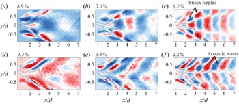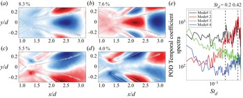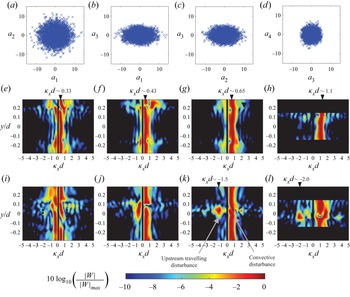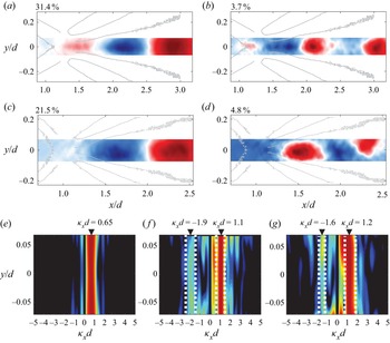


1. Introduction
Unlike its low-speed counterpart, the supersonic wake of a two-dimensional circular cylinder has not received much attention despite the rich fluid dynamics and aeroacoustic processes the flow offers. It was only recently shown (Schmidt & Shepherd Reference Schmidt and Shepherd2015) that the Mach ( $M$) 4 wake of a cylinder exhibits temporal periodicity with a higher frequency than the incompressible case. Furthermore, the Strouhal number (
 $St_d$) based on the cylinder diameter (
 $d$) and the approaching free-stream velocity (
 $U_\infty$) was observed to increase from approximately 0.3 to 0.5 as the Reynolds number (based on the cylinder diameter,
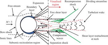
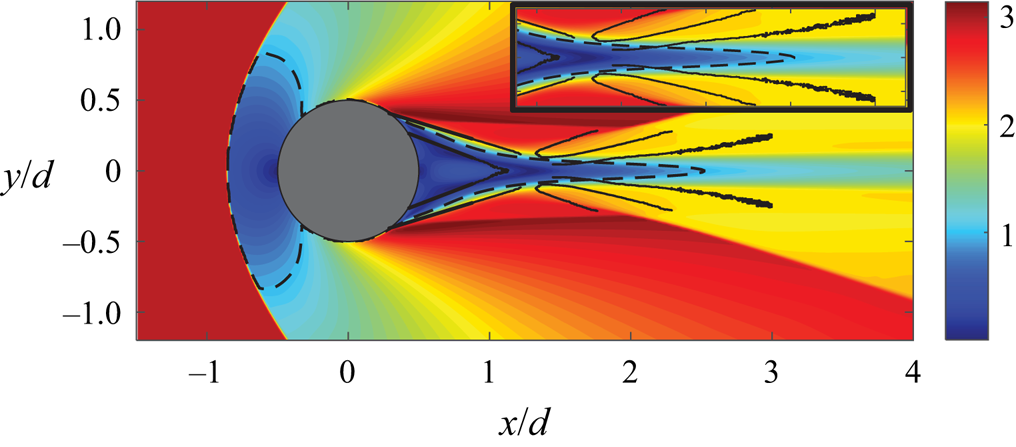
 $Re_d$) increased from approximately 20 000 to 500 000, respectively. This is perhaps not surprising when one considers that the supersonic wake of a cylinder (shown schematically in figure 1) is markedly different from the low-speed version. The wake exhibits flow features typical of supersonic planar wakes which have been studied in the past by several authors (see Bonnet, Jayaraman & Roquefort Reference Bonnet, Jayaraman and Alziary De Roquefort1984; Smith & Dutton Reference Smith and Dutton1996; Clemens & Smith Reference Clemens and Smith1998; Gai, Hughes & Perry Reference Gai, Hughes and Perry2002; Scarano & Oudheusden Reference Scarano and Oudheusden2003; Humble, Scarano & van Oudheusden Reference Humble, Scarano and van Oudheusden2007, for example). The boundary layers on the cylinder surface turn through a series of expansion waves and separate in the downstream half of the cylinder forming separated shear layers and a separation shock. Post-separation, the shear layers converge towards the wake centreline and turn to form the wake, forming a neck-like region in the process. The separated flow behind the cylinder consists of a subsonic region embedded within the supersonic flow with sonic lines (dotted lines in the figure) acting as the boundary between the two regions. The recompression of the shear layers as they turn to form the wake is accomplished through a series of compression waves that coalesce to form a recompression shock wave. The recompression process is highly unsteady due to the mutual interactions between the shear layers, the recirculation region and the recompression waves, but no studies currently exist which have characterised these dynamics in detail. Hence, the aim of the present work is to characterise the dynamic behaviour of the early wake of a circular cylinder through high-speed visualisation of the density gradient field using a focussing schlieren system. The visualised region of the wake (depicted in figure 1) includes the reattachment region, a portion of the recirculation region and the early wake (up to approximately 3.2
 $d$ downstream of the cylinder centre).
Salient features of supersonic flow over a circular cylinder. Figure not to scale.

One of the earliest works on supersonic flow over a circular cylinder was performed by Gowen & Perkins (Reference Gowen and Perkins1953), who measured the drag on cylinders for  $0.3 \leqslant M \leqslant 2.9$ and Reynolds numbers up to
 $10^6$ in the supersonic range. They found that the drag at high supersonic Mach numbers (
 $M > 1.4$) was a weaker function of Mach number and decayed slowly as the Mach number rose, suggesting a shift in the flow character at high supersonic Mach numbers. It is interesting to note that more recent measurements of the velocity field in a planar supersonic near wake (formed by a blunt base) by Humble et al. (Reference Humble, Scarano and van Oudheusden2007) have revealed that, while the dominant wake instability at Mach 1.46 is sinuous (anti-symmetric) in nature, the same wake at Mach 2.27 exhibits a varicose (symmetric) type instability. It is possible that this change in the nature of the near-wake instability is correlated with the change in drag behaviour observed by Gowen & Perkins (Reference Gowen and Perkins1953). Gowen & Perkins (Reference Gowen and Perkins1953) also acquired shadowgraph images of the flow at
 $M =1.49$ in which some of the flow structures depicted in figure 1 can be observed. Later, schlieren images taken by Murthy & Rose (Reference Murthy and Rose1977) at
 $M = 1.2$ and 1.4 with
 $Re_d = 0.166(10^6)$ also confirmed the presence of these features. Murthy & Rose (Reference Murthy and Rose1977) also measured the vortex shedding frequencies using a buried-wire gauge installed on the cylinder for a range of Mach numbers between 0.25 and 1.2 and found evidence of vortex shedding up to
 $M = 0.9$; however, above that the wire-gauge spectra were broadband, signalling a change in flow behaviour as the flow becomes supersonic.
During the 1990s, Bashkin and colleagues (Bashkin et al. Reference Bashkin, Egorov, Egorova and Ivanov1998, Reference Bashkin, Egorov, Egorova and Ivanov2000, Reference Bashkin, Vaganov, Egorov, Ivanov and Ignatova2002) studied the supersonic flow of a perfect gas over a cylinder by solving the two-dimensional Navier–Stokes equation for different flow conditions. They first showed that, for  $M$ = 5 flow over a cylinder the planar supersonic wake, features depicted in figure 1 occur for Reynolds numbers above 10 000. For Reynolds numbers below this value, they classified the flow into different regimes: separation-less flow (
 $Re_d \leqslant 250$), inception of flow separation (
 $Re_d = 275 \unicode{x2013}400$), slightly compressed separated flow (
 $Re_d = 450 \unicode{x2013}1000$) and subsonic separated flow (
 $Re_d = 1000 \unicode{x2013}10\,000$). Next, they studied both laminar and turbulent flow regimes of the cylinder wake for
 $M = 2.0$ and 5.0 (Bashkin et al. Reference Bashkin, Egorov, Egorova and Ivanov2000) and found that, for higher Mach numbers, the laminar to turbulent transition occurs at a higher Reynolds number. They found the upper limits of the transitional flow to be
 $Re_d = 5(10^4)$ and
 $10^6$ for
 $M = 2.0$ and 5.0, respectively. The Reynolds numbers in the present work (
 $6(10^5)$ and
 $7.5(10^5)$) are slightly lower than their transitional limit for
 $M = 5.0$, but given that the Mach number is also lower (
 $M = 3.0$), we expect the wake to be turbulent in the present work. Bashkin et al. (Reference Bashkin, Egorov, Egorova and Ivanov2000) also found that, for a given Mach number, an increase in Reynolds number moves the separation point on the cylinder towards the rear stagnation point and it also shortens the length of the separated flow region behind the cylinder. These observations have recently been confirmed by the shadowgraph images obtained by Schmidt & Shepherd (Reference Schmidt and Shepherd2015). Lastly, an observation from the results of Bashkin et al. (Reference Bashkin, Egorov, Egorova and Ivanov2000), which is pertinent to the present work, is that their results show that the early wake is locally subsonic at least up to 4–5 diameters downstream of the cylinder at
 $M = 2.0$. This, as will be shown in this paper, is important because it provides a pathway for an aeroacoustic resonance to develop in the wake since a subsonic flow can support both upstream and downstream propagating waves.
Based on the results described above, we have some basic understanding of the mean flow behind a circular cylinder placed in a supersonic flow. However, besides the work of Schmidt & Shepherd (Reference Schmidt and Shepherd2015), there are no studies to the authors’ knowledge which have explored the wake dynamics. As mentioned earlier, Schmidt & Shepherd (Reference Schmidt and Shepherd2015) have found the cylinder wake at Mach 4 consists of oscillations at frequency which increases with Reynolds number. They inferred a localised peak in the shadowgraph light intensity fluctuation spectra of a pixel located within the reattachment region (the neck region) as a sign of periodic oscillations in the wake. They also attempted a scaling of the peak frequencies measured at several Reynolds numbers and found that the length of the sliplines within the approaching shear layers provided the most acceptable scaling (to within approximately  $St_d = \pm 0.16$). Their choice of the slipline as the characteristic length was motivated by the fact that their Euler computations of the same flow showed an oscillation of the sliplines at the neck that appeared to be a result of a communication between the separation points on the cylinder and the end of sliplines at the neck. They proposed that this could mean that the oscillation of the sliplines which drive the periodic oscillations in the wake could be the result of acoustic perturbations that are free to travel in both upstream and downstream directions within the subsonic recirculation region. Although they did not exclude the possibility that the observed periodicity is a result of a global or a convective flow instability.
Although there is not much information on the dynamics of a cylinder wake, it is a special case of a supersonic planar wake which has been studied in the past. Thus, some insight can be gained by reviewing the existing knowledge base regarding supersonic planar wakes. The most basic of these cases is that of a wake generated by a two-dimensional blunt base, essentially a flat plate where the shear layers separate from the sharp corners at the trailing edge to form flow features similar to those shown in figure 1. Note, however, that, unlike a flat plate, the separation points on the cylinder surface are not fixed and they oscillate back and forth, as noted by Schmidt & Shepherd (Reference Schmidt and Shepherd2015). In fact, they have also suggested that this oscillation of the separation points may be linked to the vortex shedding behind the cylinder since they drive the oscillations of the sliplines embedded within the approaching shear layer.
Unlike the circular cylinder, the characteristic frequency in the wake of a blunt flat plate scales on the wake width in the case of both transitional (Lysenko Reference Lysenko1999) and fully turbulent wakes (Gai et al. Reference Gai, Hughes and Perry2002). This scaling is also independent of the Reynolds number, as evident in the large difference between the Reynolds numbers in the two aforementioned studies. This suggests that the fundamental mechanism behind the periodicity observed in the supersonic wake of a circular cylinder is different from that of a blunt flat plate wake. Regardless of these differences, it is worth considering the existing database on the behaviour of supersonic planar wakes, particularly those at high supersonic Mach numbers since they behave differently than the same wake at lower Mach numbers.
The stability characteristics of a supersonic planar wake at two different Mach numbers ( $M = 1.20$ and 2.46) was studied by Harris & Fasel (Reference Harris and Fasel1996) through direct numerical simulations (DNS). They introduced both sinuous (anti-symmetric) and varicose (symmetric) disturbances through blowing/suction slots just upstream of the plate trailing edge to determine the receptivity of these disturbances by the shear layers. They found evidence of an absolute instability at
 $M = 1.20$ with regard to sinuous disturbances, but no such instability was noted for
 $M = 2.46$ up to Reynolds number of 100 000. For the latter case, they also reported that the sinuous disturbances decayed slowly compared with the varicose disturbances. Later, Harris & Fasel (Reference Harris and Fasel1998) also considered the receptivity of the shear layers to a sinuous disturbance at several Reynolds numbers for a
 $M = 2.46$ wake and found that the wake at the Reynolds number of 250 000 exhibits a varicose-type instability even in the absence of sinuous disturbances which was not the case for lower Reynolds numbers. This varicose-type instability appears to be a typical characteristic of a high Mach number planar wake as its presence has also been reported in the Mach 2 wake of a blunt plate by Scarano & Oudheusden (Reference Scarano and Oudheusden2003). They have attributed the presence of symmetric instabilities in the wake to a pumping-type motion of the reattachment region, rather than a flapping-type motion which is associated with sinuous instabilities in low-speed wakes. The dominance of streamwise fluctuations near the reattachment region has also been observed in supersonic planar mixing layers where the Mach numbers of the two approaching shear layers are different (Smith & Dutton Reference Smith and Dutton1996; Yang, Wang & Wu Reference Yang, Wang and Wu2020). Humble et al. (Reference Humble, Scarano and van Oudheusden2007) have further shown that the flapping-type motion does exist in supersonic wakes as well, but at low Mach numbers (
 $M = 1.78$). As the Mach number is increased to 2.27 in their work, the streamwise velocity fluctuations become more elongated in the streamwise direction confirming that at high supersonic Mach numbers (of interest in the present work) the coherent structures in the wake are symmetric about the wake axis since they are generated as a result of streamwise pulsation of the reattachment region. One can presume that, in the case of the flow over a circular cylinder where the separation point is not fixed in space but oscillates back-and-forth, such a pulsating type of instability may be even stronger.
Besides the shear layers and the redeveloping wake, the other two salient flow features in the planar wake are the recirculation region and the recompression shock waves. The behaviour of the recirculation region is not well understood due to difficulties in flow visualisation closer to the base, but large reverse velocities of between 20 % and 30 % (depending on Mach number) of the free-stream velocity have been reported in this region for both planar wakes (Humble et al. Reference Humble, Scarano and van Oudheusden2007) and mixing layers (Amatucci et al. Reference Amatucci, Dutton, Kuntz and Addy1992). The temperature in this region is of the order of the stagnation temperature (Lachney & Clemens Reference Lachney and Clemens1998) and the subsonic velocities here can support bi-directional propagation of acoustic waves, which could set up an aeroacoustic resonance in the wake. Furthermore, the fluid in this region interacts with both the shear layers and the reattachment region and thus the turbulence levels here can be quite large. However, it has been shown by Humble et al. (Reference Humble, Scarano and van Oudheusden2007) that the structures here are less coherent than those in the wake or the shear layers and they attribute this lack of coherency to small-scale velocity fluctuations in this region.
The behaviour of the recompression shocks formed in planar wakes is not well understood either. It is reasonable to assume that their behaviour is inherently linked to the unsteadiness of the reattachment process. In fact, Humble et al. (Reference Humble, Scarano and van Oudheusden2007) have shown that the sinuous type of shear-layer instability which is observed at low supersonic Mach numbers causes the shocks to exhibit an alternating translation motion, whereas a varicose-type shear-layer behaviour at higher Mach numbers results in a simultaneous translation of the two shocks. It is also interesting to note that recompression shocks in an axisymmetric wake have also been shown to exhibit low-frequency unsteadiness (Simon et al. Reference Simon, Deck, Guillen, Sagaut and Merlen2007) which could also be the case for planar wakes, but to the authors’ knowledge, this has not been established. It can be presumed that the unsteady shock motion may further introduce disturbances in the wake region, affecting the flow physics.
Schlieren flow visualisation is a common tool employed to develop a qualitative understanding of complex processes in compressible flows. The technique has become even more useful recently due to the ability to capture schlieren images at a high frame rate using high-speed cameras. The high-speed schlieren images thus obtained can be analysed through a number of spatio-temporal decomposition methods such as Fourier and proper orthogonal decomposition (POD) modes. Schlieren imaging is also useful for flows with significant aeroacoustic processes since it can capture both vortical and acoustic disturbances. However, schlieren images are a result of density gradients being integrated across the entire optical path length of the system, which includes the effect of density variations within the sidewall boundary layers as well. This effect can be particularly significant for planar wakes since the three-dimensional flow separation within the sidewalls can further amplify the sidewall effects, particularly if the geometry is bluff. To minimise these effects, several studies (Weinstein Reference Weinstein1993; Garg & Settles Reference Garg and Settles1998; Lawson et al. Reference Lawson, Hargather, Settles, Weinstein and Gogineni2009; Passmann, aus der Wiesche & Joos Reference Passmann, aus der Wiesche and Joos2020) have recently employed the lens-and-grid-type focussing schlieren technique which blurs the density gradients outside a narrow plane of interest. The focussing schlieren method has been shown to minimise the sidewall effects and high-speed focussing schlieren systems can even reproduce the shape of spectra measured by a hot-wire anemometer in a supersonic turbulent boundary layer (Garg & Settles Reference Garg and Settles1998). The present work utilises both conventional and focussing schlieren visualisations of the cylinder wake performed at frame rates of up to 100 000 frames per second (fps) to compare and contrast the capabilities of the two systems.
In the present work we will discuss both the mean and unsteady characteristics of the wake behind a two-dimensional circular cylinder placed in Mach 3 flow. The main objective of the present work is to identify the behaviour and the origin of the periodic oscillations in the supersonic wake of a cylinder that were first identified by Schmidt & Shepherd (Reference Schmidt and Shepherd2015). Additionally, the study also aims to develop a comprehensive statistical description of the supersonic cylinder wake through analysis of high-speed schlieren images that may be used to better understand planar supersonic wakes and validate computational models. The region which is visualised in the present work is depicted in figure 1 and it includes the recompression shocks, the reattachment region, the redeveloping wake and a portion of the recirculation region and the approaching shear layers. The flow visualisations were performed for two different diameter cylinders with  $Re_d = 6(10^5)$ and 7.5(
 $10^5$). The flow field was visualised through both high-speed conventional and high-speed focussing schlieren systems. For the former, only the density gradient in the vertical direction was visualised, while for the latter, the visualisation of the density gradients in both vertical and streamwise directions was performed. The remaining paper is organised as follows. The facility and the two schlieren systems are described first in § 2. This section also presents the results of separate measurements undertaken to establish the depth of field of the focussing schlieren system and the methodology used to post-process the schlieren data. Next, the salient flow features of the cylinder wake are discussed through an analysis of the instantaneous, mean and variance images extracted from the schlieren datasets in § 3.1. Here, we also compare and contrast the capabilities of the two schlieren systems. This is followed by a discussion of the unsteady flow characteristics of the wake in § 3.2. In § 3.3 we reveal the presence of aeroacoustic resonance in the wake, which results in the formation of a standing wave type of pattern. The coherent structures in the wake obtained through POD of temporally filtered schlieren datasets are discussed in § 3.4. The aeroacoustic resonance in the cylinder wake is then revisited in § 3.5, where the mechanism behind the standing wave formation in the wake is presented before concluding the paper in § 4.
2. Experimental set-up
2.1. UNSW supersonic wind tunnel and circular cylinders
The measurements were performed in the Mach 3 Supersonic Wind Tunnel at the University of New South Wales (UNSW). The facility is a blowdown to atmosphere-type wind tunnel capable of providing a sustained Mach ( $M$) 3 flow for approximately 16 s in a
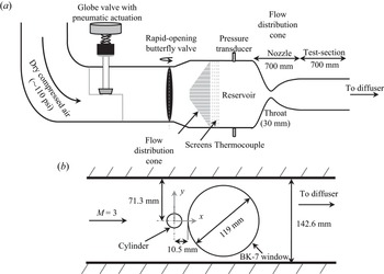
 $142.6\ {\rm mm}\times 101.6\ {\rm mm}$ rectangular test section. Figure 2(a) shows a side-view schematic of the facility. The atmospheric air is compressed using an Ingersroll Rand
 CENTAC compressor, dried and then stored in storage tanks which are separated from the rest of the facility through a tunnel isolation valve. Downstream of this valve, a pneumatically actuated globe valve (figure 2a) regulates the stagnation pressure of the tunnel. Further downstream, a rapid-opening butterfly valve serves as the tunnel operation valve. Once this valve is opened, the air is conditioned through an air distribution cone and four turbulence reduction screens before entering a circular cross-section reservoir with a diameter of 336.5 mm. The reservoir pressure and temperature of the facility are monitored using a
 $150\pm 1.5$ psia
 A – 10 pressure transducer and a K-type thermocouple, respectively. Downstream of the reservoir, the flow is accelerated through a two-dimensional converging–diverging nozzle to Mach 3 in the test section. The nozzle throat is 30 mm wide and the test-section to throat area ratio is 4.75. The test-section length with Mach 3 flow, as determined using static pressure taps along the wall, is approximately 700 mm. Downstream of the test section, the flow is diffused, first through a parallel supersonic diffuser, and then through a diverging, subsonic diffuser section. The flow is then turned three times through an acoustically lined rectangular duct before being exhausted into the laboratory at low subsonic speeds. More details of this facility can be found in Wills et al. (Reference Wills, Awasthi, Doolan and Moreau2019).
(a) UNSW Mach 3 supersonic wind tunnel. (b) Schematic showing cylinder set-up in the test section along with optical access window. The figure is not to scale.

The test-section static pressure is monitored using a  MKS750C pressure transducer with a range of
 $172.37 \pm 0.17\ {\rm kPa}$. The test-section Mach number and Reynolds number are calculated using isentropic relationships. During the tunnel operation, the stagnation pressure varies with time which changes the flow Reynolds number in the test section. This change in Reynolds number is highly repeatable and is well characterised. In the present work, all measurements were triggered when the stagnation pressure in the reservoir reached 600 kPa. The high-speed schlieren videos (discussed below) were taken for 2.2 s during which the Reynolds number (per unit length) varies between
 $50(10^6)$ and
 $52(10^6)$. The Mach number, however, remains nearly constant during the measurement window. Based on the uncertainty in pressure and temperature measurements, the uncertainty in Mach number estimation is
 $\pm$0.013 while that in Reynolds number (per unit length,
 $Re_L$) is
 $\pm$500.
Two different cylinders machined from aluminium with diameters ( $d$) of 12 mm and 15 mm were used in the present work. The Reynolds numbers based on the cylinder diameter (at the start of measurement trigger) are
 $Re_d = 6.0(10^5)$ and
 $7.5(10^5)$ for
 $d = 12$ mm and 15 mm, respectively. The cylinders were mounted at the mid-height of the test-section, 292 mm downstream of the nozzle throat, and spanned the entire width (101.6 mm) of the test section. The side-view schematic of the test section in figure 2(b) shows the cylinder mounted in the test section. A 119 mm diameter circular window made from schlieren grade BK-7 glass was mounted immediately downstream of the cylinder in order to visualise the cylinder wake through schlieren flow visualisation (discussed in the next section). For both the cylinders, the optical window was located such that its most upstream edge was 10.5 mm from the centre of the cylinders. This implies that the very near-wake region of the cylinder (approximately
 $0.38d$ and
 $0.2d$ downstream of the cylinder base for
 $d = 12$ mm and 15 mm, respectively) is not visible in the flow visualisations. Figure 2(b) also shows the
 $x-y$ coordinate system which will be followed throughout the text. The origin of the coordinate system in the spanwise direction (
 $z$) is located at the spanwise centre of the test section.
2.2. Conventional and focussing schlieren systems
Two different types of high-speed schlieren imaging systems – a conventional, z-type system and a focussing schlieren system – were employed to visualise the wake. The conventional schlieren system was used to visualise only the vertical density gradient ( $\partial \rho /\partial y$) field, while the focussing schlieren system was used to visualise both the vertical and the streamwise (
 $\partial \rho /\partial x$) density gradients. As discussed momentarily, the focussing schlieren system is better suited to visualising planar wake flows as it suppresses the image contamination due to strong density gradients in the sidewall boundary layer; however, the conventional schlieren system offers a larger field-of-view (fov) which can be utilised to complement the results derived from the former. In both cases, high-speed images up to 100 000 fps were acquired allowing detailed spatio-temporal analysis of the wake features.
The conventional schlieren system used here to visualise the wake was recently used by Zhang et al. (Reference Zhang, McCreton, Awasthi, Wills, Moreau and Doolan2021) to study transverse jets in supersonic cross-flow and the details of this system can be found there. The schlieren videos were recorded using a monochromatic, MEMRECAM HX-7s high-speed camera. The camera was set to automatically start acquiring images once the test-section Mach number and the reservoir pressure reached a preset value (600 kPa). The conventional schlieren images were acquired at a frame rates of 60 000 fps and 100 000 fps with a pixel resolution of  $320\times 160$ and
 $320\times 88$, respectively. In terms of dimensional spatial resolution, this corresponds to approximately 0.24 mm per pixel and 0.11 mm per pixel, respectively in both directions. The resulting greyscale pixel intensities in each schlieren image frame were then post-processed using the methodology described in § 2.4.
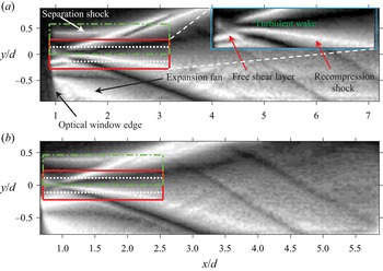
Figures 3(a) and 3(b) show the mean schlieren images of the 12 mm and 15 mm cylinder wakes, respectively obtained by averaging  $2^{14}$ instantaneous schlieren frames. Each image shown here was subjected to a pixel-wise low-pass Weiner filter to minimise high-frequency camera noise after which an edge-aware, fast local Laplacian filter as described in Paris, Hasinoff & Kautz (Reference Paris, Hasinoff and Kautz2015) was applied to each image in order to improve the details in the image. Finally, a histogram equalisation was applied to each image to improve the contrast. Same post-processing methodology was applied to every instantaneous or mean schlieren image shown throughout the rest of the paper. The mean images show the typical flow features expected from a planar supersonic wake, however, the features are not well resolved due to both the low resolution of the images and the fact that the low Mach number separation from the cylinder in the sidewall boundary layers blurs the two-dimensional flow features. The superimposed rectangles on the mean images depict the fov for the focussing schlieren system which is described next.
Mean schlieren images for (a) 12 mm cylinder and (b) 15 mm cylinder obtained using the  $z$-type, conventional schlieren imaging system. Inset in (a) shows a close-up of the early wake of the cylinder. The three superimposed rectangles show the fovs of the three different focussing schlieren datasets for each cylinder.

To overcome the end-effect contamination of the conventional schlieren system, as well as to gauge its performance for flows with strong end effects, lens-and-grid-type high-speed focussing schlieren system (based on the concept proposed by Weinstein Reference Weinstein1993) was also used to visualise the flow behind the cylinder. A focussing schlieren system is sensitive to density gradients within a finite plane perpendicular to the optical axis of the system (the plane of focus) and the density gradients outside this plane are blurred. The theoretical performance of a focussing schlieren system and the related design issues have recently been discussed in detail by several authors (Lawson et al. Reference Lawson, Hargather, Settles, Weinstein and Gogineni2009; Passmann et al. Reference Passmann, aus der Wiesche and Joos2020; Martinez-Gonzalez et al. Reference Martinez-Gonzalez, Moreno-Hernandez, Guerrero-Viramontes, Leon- Rodriguez, Zamarripa-Ramirez and Carrillo-Delgado2018), so here only the set-up, performance and the capability of the present system are described.
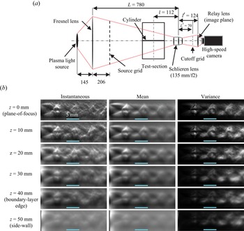
Figure 4 shows the optical component arrangement of the focussing schlieren system as it was used in the present work and table 1 provides the specifications of each optical component utilised in the system. The system is backlit using the same plasma light source as the conventional schlieren system (see Zhang et al. (Reference Zhang, McCreton, Awasthi, Wills, Moreau and Doolan2021) for a description of the conventional schlieren system), however, a Fresnel lens/source grid arrangement is placed in front of this source which then acts as the effective source of the system. The purpose of the Fresnel lens is to enhance the brightness of the system. The source grid consists of alternating opaque and transparent lines which both have the same thickness (2 mm) in the present work. The light from the line sources passes through the test section and is focused on to a cutoff grid (photonegative of the source grid) using a schlieren lens on the other side of the test section. The cutoff grid had a spacing of 0.3 mm between the alternating clear and opaque lines. The locations of the source and cutoff grids with respect to the schlieren lens are fixed by the grid sizes and the lens magnification. The ability of the schlieren lens to focus on a plane between the source and the cutoff grid provides the system its focussing capability. A plano-convex relay lens placed behind the cutoff grid was then used to focus the image on the sensor of the high-speed camera. The relay lens acts as the image plane of the system and it was moved relative to the schlieren lens along the optical axis to bring different planes into focus. The plane of focus for the imaging of the cylinder wake was centred at the spanwise centre of the test section, however, it was also adjusted to assess the focussing capability of the present system as described below.
The focussing schlieren imaging system. (a) Schematic showing the optical components and their placement. Here, the flow is out of the page and all dimensions shown are in mm. (b) The instantaneous (left column), mean (middle column) and variance (right column) images with different spanwise location of the jet centreline. The spanwise location corresponding to each row is shown to the left. The horizontal line near the bottom of each image corresponds to a length scale of 5 mm.

Focussing schlieren component specifications.

The plane of focus of a focussing schlieren system has a finite depth (referred to as the depth of field ( $DU$) in the focussing schlieren literature) which must be established to assess the extent to which it can blur the density gradients outside the region of interest. In order to assess the depth of field of the present system, an experiment where an underexpanded jet of air was traversed along the optical axis within the test section of the facility was undertaken. The underexpanded jet was issued from a 4.8 mm diameter (
 $d_n$) convergent nozzle into the ambient air and the resulting schlieren images were recorded at 12 000 fps with a
 $1024 \times 1024$ pixel resolution, and an exposure time of
 $0.6\ {\mathrm {\mu }}{\mathrm {s}}$. The plane of focus in these measurements was centred at the spanwise centre of the test section (
 $z = 0$) and schlieren images with the jet centreline located at several spanwise stations were recorded to reveal the focussing capability of the system. Figure 4(b) shows the instantaneous (left column), mean (middle column) and variance (right column) images for six spanwise locations of the jet (§ 2.4 describes the methodology used to calculate the mean and variance from schlieren images). Both the mean and the variance images show well-defined flow features (shock cells and shear layers) in the plane of focus which blur as the jet traverses away from the test-section centre towards the sidewalls. The blurring is more significant for features located further downstream since they impose weaker density gradients and become wider as the jet spreads. When the jet is located near the sidewall (
 $z = 50\ {\rm mm}$), the shock cells and the shear layers are barely visible in either of the images. Note that the jet location of
 $z = 40\ {\rm mm}$ corresponds approximately to the edge of sidewall boundary layer and a rapid deterioration in the image sharpness is observed between this point and the sidewall location. This suggests that the present system is well suited to visualise the spanwise-averaged density gradients within the two-dimensional portion of the wake.
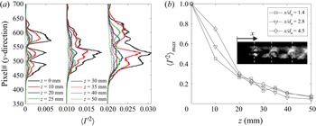
The depth of field of the present system is further analysed in figure 5 through an analysis of the variance of the pixel intensity values (see § 2.4 for a definition of the variance) contained within the focussing schlieren images. Figure 5(a) shows the variance along the three vertical dashed lines shown in figure 5(b) inset for different jet spanwise locations. These vertical lines are located approximately 1.4, 2.8 and 4.5 jet diameters downstream of the nozzle exit. The variance curves for  $x/d_n = 2.8$ and 4.5 have been scaled by a constant value to show them on the same plot. In each case, the variance peaks within the jet and it decreases as the jet travels away from the plane of focus. A smoothing of the variance peaks can also be observed beginning around
 $z = 20\ {\rm mm}$. The variance values in proximity to the sidewalls (
 $z=40\ {\rm mm}$ and 50 mm) are closer to those observed outside the jet core than those within the jet in the focus plane. Figure 5(b) shows the variation of maximum variance found along the three lines as a function of spanwise jet location. The schlieren images lose approximately 90 % of the variance as the jet approaches the sidewall boundary layer. This suggests that we can expect the sidewall effects to be negligible in any mean-square statistics (e.g. Fourier spectrum) extracted from the high-speed schlieren images using the present set-up. In § 3.1 we show a direct comparison between the conventional and focussing schlieren images of cylinder wake which further highlight the superior performance of the latter in visualising flows with strong end effects.
Depth of field assessment for the focussing schlieren system through pixel variance of the underexpanded jet. (a) Variance along the three vertical lines shown in (b) inset for different jet spanwise locations. (b) Maximum variance along the vertical lines in inset as a function of spanwise jet location.

2.3. The field of view of the focussing schlieren system
The focussing schlieren set-up has a smaller fov than the conventional schlieren set-up due to the magnification being fixed by the grid sizes and the schlieren lens used in the assembly. Furthermore, a higher sampling rate requirement can further reduce the fov due to the on-board camera memory limitation. Therefore, to ensure that all relevant parts of the cylinder wake were visualised with sufficient spatio-temporal resolution, the entire optical assembly was physically translated in the  $x$ and
 $y$ directions to image three different regions which were previously highlighted in figures 3(a) and 3(b). Table 2 provides the image resolution, sampling rate and the spatial extent of each of these regions along with the terminology which will be used to refer to these regions during the discussion of the results. The 50k near-wake and the 100k near-wake regions have the same streamwise extent, but the latter has a shorter spanwise extent due to a higher sampling rate. The 50k upper-wake region covers only the upper half of the wake so that the behaviour of the approaching shear layer, the recompression shocks and their interaction can be visualised in greater detail. For each fov, both the vertical gradient and the streamwise gradient of the density were visualised by placing the cutoff grid in horizontal and vertical orientations, respectively.
Details of the focussing schlieren fov shown in figure 3.

2.4. Post-processing of high-speed schlieren videos
The schlieren videos recorded through both the schlieren systems yield frames which contain a pixel intensity value ( $I(x,y)$) between 0 and 1 which corresponds to black and white colours, respectively. Thus, each schlieren video acquired in the present work yields a three-dimensional matrix (
 $\boldsymbol {I}(x,y,t)$) of size
 $N_x \times N_y \times N$, where
 $N_x$ and
 $N_y$ are the number of pixels in the
 $x$ (streamwise) and
 $y$ (vertical) directions, respectively, and
 $N$ is the total number of frames. Then, the schlieren frames can be processed using any spatio-temporal data reduction technique with the understanding that the results represent the behaviour of the density gradients (either streamwise or vertical) averaged over some spanwise distance. In the case of conventional schlieren, this spanwise depth is equal to the entire optical path length, whereas for the focussing schlieren it is approximately the depth of the two-dimensional flow within the test-section. Before further processing of the schlieren data, each frame in the schlieren videos was subjected to a pixel-wise low-pass Weiner filter to minimise high-frequency camera noise. The local mean and the standard deviation required for the Wiener filter was calculated using a subset of
 $4 \times 4$ pixels. For each schlieren dataset, a mean and a variance image was formed by calculating the temporal mean (
 $\langle \boldsymbol {I}(x,y)\rangle$) and the variance (
 $\langle \boldsymbol {I}'^2(x,y)\rangle$), respectively of the light intensity in each pixel from
 $2^{14}$ frames. A spectral analysis of the schlieren data (presented in § 3.2) was also performed by calculating the auto and cross-spectral densities between the fluctuating light intensities of the pixels (
 $\boldsymbol {I'}(x,y)$). The spectral parameters in each case were estimated through the periodogram method by dividing the schlieren data matrices into blocks with 256 frames per block, a Hanning window was applied to each block and an overlap of 50 % between the blocks was used to increase the number of records for averaging.
The fluctuating light intensity in each pixel of the schlieren images were also decomposed into a set of orthogonal modes using POD. The POD algorithm seeks to decompose a spatio-temporal, zero-mean dataset into a linear combination of spatial modes ( $\boldsymbol {\phi }$) modulated by temporal coefficients (
 $a_i$) as
 \begin{equation} \boldsymbol{I}'(x,y,t) = \sum_{i=1}^N a_i(t)\boldsymbol{\phi_i}(x,y). \end{equation}
Here, the snapshot POD method of Sirovich (Reference Sirovich1987) was used to calculate the POD spatial modes and the temporal coefficients since the spatial dimension of the data is large. The spatial modes were calculated by first performing an eigendecomposition of the schlieren light intensity fluctuation cross-correlation matrix which is defined as
 \begin{equation} \boldsymbol{C} = \frac{1}{N-1}\boldsymbol{J}'\boldsymbol{J}', \end{equation}
where,  $\boldsymbol {J}'$ is the data matrix of size
 $N \times M$ which contains the schlieren light intensity fluctuations within
 $M$ pixels for
 $N$ number of temporal points. The
 $N$ eigenvalues of the correlation matrix represent the fractional energy contribution of each mode towards the energy contained in the whole dataset. The eigenvalues are arranged in descending order such that the first and the last eigenvalues represent the most and the least energetic modes, respectively. The
 $N$ eigenvectors of the correlation matrix are the temporal modes which are then projected on the data matrix (
 $\boldsymbol {J}$) to yield the spatial POD mode matrix (
 $\boldsymbol {\varPhi }$) as
 \begin{equation} \boldsymbol{\varPhi} = \boldsymbol{J}'\boldsymbol{\varPsi}, \end{equation}
where  $\boldsymbol {\varPsi }$ is the eigenvector matrix of the data matrix
 $\boldsymbol {J}$ which is formed by arranging the individual eigenvectors in order of decreasing energy. Each eigenvector is also normalised such that its length is unity such that the spatial modes are consistent with the results obtained from the direct POD. The POD temporal coefficients (
 $a_i(t)$) are then obtained by projecting the data matrix on the spatial POD modes as
 \begin{equation} \boldsymbol{A} = \boldsymbol{J}\boldsymbol{\varPhi}, \end{equation}
where,  $\boldsymbol {A}$ is the matrix whose columns consist of temporal coefficients for each mode.
2.5. The effect of flow three-dimensionality on schlieren imaging
Before we delve into the discussion of the statistics obtained from the schlieren imaging, a discussion on the effect of any three-dimensionality of the flow on the schlieren images is warranted since schlieren images are a two-dimensional representation of a three-dimensional phenomenon. Therefore, the results from the present measurements must be interpreted considering this limitation. In a two-dimensional or a quasi-two-dimensional flow (e.g. axisymmetric wakes and jets), the averaged schlieren statistics will be biased towards the two-dimensional flow structures owing to their spanwise organisation since incoherent fluctuations in the third dimension will be averaged out. However, if the flow is three-dimensional, the schlieren images may not yield a true representation of the scales associated with the flow structures. In the context of the present work, the three-dimensional disturbances that may influence the schlieren images are expected to be of two types. The first type are the coherent structures in the wall-normal directions within the sidewall boundary layer. Although the focussing schlieren system minimises the disturbances due to the sidewall boundary layer, it does not eliminate them. It has been shown previously that three-dimensional effects due to the sidewalls may be significant for flows with a large embedded separated flow region and reattachment such as mixing layers (Amatucci et al. Reference Amatucci, Dutton, Kuntz and Addy1992) and flow over a compression ramp (Kuntz, Amatucci & Addy Reference Kuntz, Amatucci and Addy1987). In case of the latter, the reattachment was observed to be two-dimensional at least over the middle 70 % of the test section. Although it is difficult to ascertain the exact wall-normal extent of the three-dimensional flow region near the cylinder/sidewall junction without spanwise flow visualisation, it is reasonable to assume that this extent would be larger than the height of the incoming boundary layer thickness. In fact, a recent instantaneous flow visualisation of a Mach 3.8 flow over a cylinder with free end mounted to a wall (Gang, Yi & Niu Reference Gang, Yi and Niu2021) appears to show sparse, but large coherent structures whose wall-normal extent can reach approximately twice the incoming boundary layer thickness (although the extent of the contribution of the free end to these structures is unclear). These facts imply that in the present case the wall-normal extent of the three-dimensional flow near the cylinder/wall junction may be somewhere between 15 % and 20 % of the test-section width. Even if this is the case, the results of the focusing schlieren system assessment in figure 5(b) show a loss of approximately 80 % of the variance associated with the three-dimensional structures. Additionally, because the depth of the two-dimensional flow region will be much larger than that of the three-dimensional region, this suggests that the sidewall influence on the mean-square statistics derived from the schlieren images can be expected to be negligible.
The second type of three-dimensionality that may influence the schlieren statistics comes from the presence of any three-dimensional coherent structures within the cylinder wake itself. These structure, when present, will be smeared out in schlieren images due to the light path integration offered by the schlieren imaging. It has been shown that in compressible mixing layers three-dimensional instabilities appear in form of oblique waves and they become the dominant feature of the flow field as the compressibility increases (Smith & Dutton Reference Smith and Dutton1996; Sandham & Reynolds Reference Sandham and Reynolds2006). The presence of such structures in compressible planar wakes has not been studied extensively to the authors’ knowledge, however, a recent study on transitional planar wakes (Hickey, Hussain & Wu Reference Hickey, Hussain and Wu2016) has shown that increasing compressibility promotes two-dimensionality in the flow which is the opposite of what happens in a compressible mixing layer. In yet another recent study on the supersonic wake of a wedge (Li Reference Li2022), three-dimensional structures were found to exist in the near wake. Thus, there is some degree of uncertainty whether three-dimensional flow structures such as oblique waves are an inherent feature of a planar supersonic wake. Regardless, if these structures do exist they may give a false impression of two-dimensionality in the schlieren images. In the context of the present work, we are mainly interested in the periodicity of coherent structures in the wake and we believe that, while any three-dimensionality of the flow will smear out the flow structures, it should not affect the main conclusions reached in this paper. It is also noteworthy that in regions where three-dimensionality is the dominant flow feature, any modal decomposition method such as POD which is used here would yield flow structures that are not as sharp as in the two-dimensional case since POD relies on the spatial coherency between the schlieren light intensity fluctuations. In fact, a difficulty in the interpretation of POD eigenvectors of velocity fluctuations in a planar supersonic wake has partially been attributed to the possible presence of three-dimensional, oblique instabilities (Humble et al. Reference Humble, Scarano and van Oudheusden2007) (although the authors admit that low seeding volume in these three-dimensional flow regions may also be a contributing factor). It is also worth noting that the schlieren images capture density gradients in one direction (either horizontal or vertical) and will therefore not be able to capture flow structures that produce density gradients aligned parallel to the cutoff grid. Whilst this density gradient information may be lost, we believe the remaining density gradients that are not perfectly aligned to the cutoff grid will produce enough information to analyse the density gradients in both the streamwise and spanwise directions.
3. Results and discussion
We will now develop and discuss a statistical description of the supersonic wake behind a circular cylinder as obtained through spatio-temporal analysis of the schlieren datasets. The 12 mm cylinder will serve as our baseline case due to its larger fov in terms of cylinder diameter and the results from the 15 mm cylinder will be shown as necessary. Also, the imaging sensitivity and range for both the schlieren systems were tuned to the 12 mm cylinder wake, thus the visualisation results for this cylinder are in general superior. Unless otherwise stated, the analysis will utilise the focussing schlieren datasets. The mean and instantaneous flow field behind the cylinder will be discussed first. This will be followed by a spectral analysis of the density gradient fluctuations in the cylinder wake. We will then provide evidence of aeroacoustic resonance which occurs in the wake and this will be followed by a discussion on the coherent oscillations within the wake. Finally, the mechanism behind the aeroacoustic resonance observed in the wake will be explained.
3.1. Mean and instantaneous flow fields
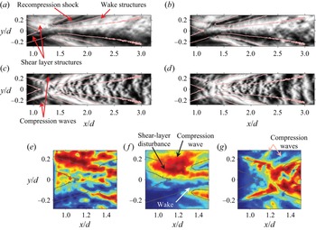
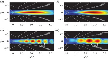
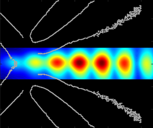
We first consider the instantaneous wake flow field as captured by the two focussing schlieren systems (horizontal and vertical knife-edge systems) as shown in figure 6(a–d). Each pair of the schlieren images in the top and the bottom rows show two consecutive snapshots of the wake flow field as imaged by the horizontal knife-edge and vertical knife-edge systems, respectively. The aspect ratio of each image is 4 : 1 and the lines superimposed upon each image highlight the approximate mean boundaries of the shear layer, the recompression shocks and the wake. These boundaries were obtained through a custom edge-detection algorithm applied to the focussing schlieren variance images which will be described later in this section. Both the horizontal knife-edge focussing schlieren (figure 6a,b) and the vertical knife-edge focussing schlieren (figure 6c,d) snapshots have been taken from the 50k near-wake dataset (see table 2 and figure 3).
Two consecutive instantaneous schlieren snapshots from the horizontal knife-edge focussing schlieren (a,b) and the vertical knife-edge focussing schlieren (c,d). The time between the snapshots is 0.02 ms. A close-up view of the instantaneous field near the shear-layer reattachment from the conventional schlieren, horizontal knife-edge focussing schlieren and vertical knife-edge focussing schlieren is shown in (e–g), respectively. The snapshots in (e–g) have been recoloured to RGB such that red, blue and green colours represent white, black and grey pixels, respectively.

Now consider the wake flow features revealed by the instantaneous images. Each dataset shows that the flow field is highly unsteady and consists of several convective as well as acoustic features. The turbulent structures within the wake and the approaching shear layers can be more clearly observed in the focussing schlieren vertical density gradient images (a,b), while the streamwise density gradient images from focussing schlieren (c,d) show wave-like features which curve in the downstream direction between the wake and the recompression shocks. Several compression waves over-riding the approaching shear layer can also be observed in these images. The affinity of vertical knife-edge schlieren towards revealing large-scale, wave-like disturbances in a planar wake has also been previously observed in schlieren images of a Mach 2 flat plate (Gai et al. Reference Gai, Hughes and Perry2002). Furthermore, the images in figures 6(c) and 6(d) also bear a remarkable resemblance to the streamwise density gradient field of a Mach 2.46 axisymmetric wake computed using DNS (Sandberg Reference Sandberg2012). These results suggest that in the present measurements, the horizontal knife-edge configuration is better suited to visualising turbulent flow structures than the vertical knife-edge set-up. This is perhaps also the reason why the light intensity fluctuation spectrum from a high-speed horizontal knife-edge focussing schlieren has been found to have the same shape as a spectrum measured in a boundary layer using a hot-wire (Garg & Settles Reference Garg and Settles1998).
Figure 6(e–g) offers a close-up view of the free shear layers and their reattachment captured by both the conventional schlieren system (figure 6e) and the focussing schlieren system (figure 6f,g). The focussing schlieren images are a trimmed version of the snapshots shown in figure 6(a–d), while the conventional schlieren image was extracted from a set of images acquired at 60 000 fps and it was trimmed to the same physical size as the focussing schlieren images. The conventional schlieren snapshot (figure 6e) shows the structures in the approaching shear layers, however, it also shows myriads of finer structures which may be attributed to the contamination of the schlieren image by the turbulence along the sidewalls. On the other hand, the disturbances within the approaching shear layer and the redeveloping wake are easier to identify in the horizontal knife-edge focussing schlieren image in figure 6( f). The redeveloping wake in the vertical knife-edge focussing schlieren image (figure 6g) is not as clearly defined, but the approaching shear layer and several compression waves riding on it can be observed in this image. These compression waves appear to be related to the shear-layer vorticity and their appearance is reminiscent of the Mach radiation observed in high-speed jets (Fujii, Nonomura & Tsutsumi Reference Fujii, Nonomura and Tsutsumi2010; Nonomura & Fujii Reference Nonomura and Fujii2011; Bailly & Fujii Reference Bailly and Fujii2016) that has been studied widely since they can lead to aeroacoustic resonance phenomenon known as screech (Edgington-Mitchell et al. Reference Edgington-Mitchell, Wang, Nogueira, Schmidt, Jaunet, Duke, Jordan and Towne2021). Unlike high-speed jets, however, the compression waves observed here are inclined in the downstream direction since the ambient flow is supersonic, and assuming the shear-layer vorticity acts like a wavy wall, these are left-running characteristics, instead of right-running characteristics when the ambient flow is subsonic. Additionally, unlike the Mach waves in high-speed jets that can propagate upstream outside the jet and lead to the formation of an aeroacoustic feedback loop, the present compression waves can only propagate downstream. Regardless of these differences, it is shown later in § 3.5 that these compression waves may still lead to aeroacoustic resonance in the cylinder wake as they find an indirect pathway for upstream propagation through the subsonic portion of the redeveloping wake and the recirculation region.
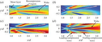
Figure 7 shows the mean (a,c) and the variance (b,d) images behind the 12 mm cylinder from the horizontal knife-edge focussing and conventional schlieren systems. The mean images have been converted to RGB format for clarity with red, green and blue corresponding to white, grey and black pixels, respectively. The variance images also follow the RGB format with blue and red coloured pixels representing the lowest and highest variance, respectively within any given image. First consider the mean schlieren images in figure 7(a,c). The conventional schlieren mean image (figure 7a) highlights the salient features of the flow field successfully. The gradients are strongest around the recompression region and in the outer parts of the shear layer and the wake. The mean images from the horizontal knife-edge focussing schlieren (figure 7c) has a similar appearance to the conventional schlieren mean image, but the image has sharper features. The advantage of using a focussing schlieren system to visualise the cylinder flow becomes apparent when one considers the schlieren variance images from the conventional and focussing schlieren systems as shown in figure 7(b) and (d), respectively. The conventional schlieren variance image (figure 7b) captures the unsteady motions in the recompression region, however, the wake and the shear layers are contaminated by the end effects. On the other hand, the horizontal knife-edge focussing schlieren (figure 7d) clearly shows the wake growing from the reattachment region along with significant unsteadiness around the recompression region. Note that the closed curve defining the recompression region displays significant unsteadiness at its upstream and downstream boundary. These two unsteady features are believed to be associated with the oscillations of the leading and trailing boundaries of the compression wave train (sometimes referred to as the shock foot in the literature) which ultimately coalesces to form the recompression shock further away from the cylinder (see figure 1). The unsteadiness of these boundaries is also visible in the Euler computations of Mach 4 cylinder wake by Schmidt & Shepherd (Reference Schmidt and Shepherd2015) where a significant movement of the shock foot can be observed. The approaching shear layer is not readily visible in figure 7(d) due to the relatively low fluctuations within them when compared with the wake and the recompression wave region.
Mean (a,c) and variance (b,d) of pixel intensity in schlieren images for the 12 mm cylinder wake. (a,b) Horizontal knife-edge conventional schlieren and (c,d) horizontal knife-edge focussing schlieren. The focussing schlieren images were obtained from the 50k near-wake dataset, while the frame rate of the conventional schlieren images was 60 000 fps.

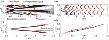
Before we leave this section to discuss the unsteady flow field behind the cylinder, we consider some relevant geometric scales in the cylinder wake estimated using a custom edge-detection algorithm. Recall that the edges generated by this algorithm were already shown on the mean and instantaneous images discussed above, and these edges will be utilised extensively throughout this paper to provide a spatial reference. Considering the mean schlieren images in figure 7, it is clear that the variance image computed from the horizontal knife-edge focussing schlieren data (figure 7d) is most suited to calculating the edges as it provides a clear distinction between the different flow features (shear layers, wake and the recompression wave). Since the boundaries of these features are associated with a sharp local change in the variance, the phase of the gradient of the variance image was used to estimate these boundaries. The image gradient was calculated using a central difference scheme and figure 8(a) shows the phase of the variance image gradient vector for the 12 mm cylinder extracted from 50k near-wake horizontal knife-edge schlieren dataset. The phase image has been binarised such that positive phase values are represented by 1 and negative values are represented by 0. The binary phase image reveals the flow structures and their boundaries with more clarity since the variance along these boundaries is changing rapidly. Note that the phase of the same feature (e.g. wake) has an opposite sign about the axis of symmetry. Next, the edges of these features were determined by finding the pixel values where the change in sign of the phase occurs. These pixels, which have been superimposed upon the binary phase image, yield the edges of the flow features in the flow field as well as several spurious edges which were manually deleted. The horizontal knife-edge schlieren dataset yields reliable edges for the recompression region and the wake; however, there is some ambiguity in the shear-layer edges due to the low variance values. Thus, the edges depicting outer boundaries of the shear layer were extracted from the vertical knife-edge schlieren variance images (figure 6g) using the same edge-detection method described here. Note that there is some asymmetry in the edges about the axis of symmetry due to the cutoff grid not blocking exactly 50 % of the light from the source grid. In instances where the edges detected by the gradient method are spurious or incomplete, the edges of the same feature on the opposite side were reflected about the axis of symmetry for a complete image.
Variance image gradient based edge-detection method. (a) Binary image of the phase of the variance image gradient vector with superimposed edges for the 12 mm cylinder. (b) Wake boundary identification through local minimum variance along several streamwise stations in the wake of 12 mm cylinder. (c) Wake boundaries for the 12 mm cylinder using edge-detection method and polynomial fit. (d) Mean wake-width comparison between the 12 mm cylinder (black curve) and 15 mm cylinder (red curve) using the edge-detection method (lines) and the local minimum variance method (symbols). For each image shown here, the 50k near-wake dataset was utilised.

The edge-detection method was validated by comparing the wake thickness yielded by the variance image gradient based method with that obtained by assuming that a local minimum in variance along the vertical direction represents the mean wake boundary. Figure 8(b) shows a line plot of variance in the vertical direction at several streamwise locations in the 12 mm cylinder wake. A total of 11 profiles at streamwise station between  $x/d = 1.38$ and 2.5 with increments of
 $\Delta x/d = 0.11$ between the stations are shown. Each profile shows a maximum near the wake centreline and a local minimum on either side (highlighted using filled circles). This local minimum shifts outwards as the wake grows and its location was used to calculate the wake thickness as a function of streamwise distance for both the cylinders. Next, the wake thickness was also calculated by fitting a polynomial curve to the wake boundaries yielded by the edge detection method discussed previously. A third-order polynomial was found to provide the best fit (in a least-squares sense) to the wake edge data. Figure 8(c) shows the wake boundaries for the 12 mm cylinder from the edge-detection method along with a polynomial fit. The wake thickness was then estimated by calculating the distance between the two polynomial fits. Figure 8(d) shows the wake thickness as a function of streamwise distance for the two cylinders using both methods. The two methods yield nearly identical results, but the edge-detection method is easily automated. The wake width for the 15 mm cylinder has a slightly steeper rise near the wake origin, but beyond approximately
 $x/d > 1.4$, it has nearly the same growth rate as the lower Reynolds number wake.
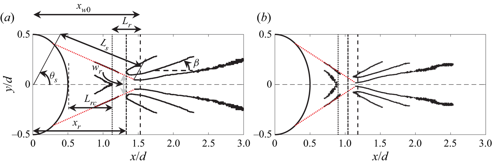
Figures 9(a) and 9(b) show the edges depicting boundaries of the salient flow features in the wake of the 12 mm and 15 mm cylinders, respectively along with the downstream half of the cylinder itself. Figure 9(a) shows the definition of several geometric parameters which were estimated from these edges. The estimated values of these parameters for both the cylinders are shown in table 3. The lengths  $L_s$,
 $L_{rc}$ and
 $L_r$ are the mean shear-layer length, recirculation region length and the reattachment region length, respectively. The streamwise locations
 $x_{w0}$ and
 $x_r$ are the approximate streamwise locations of the wake origin and mean reattachment point respectively measured from the centre of the cylinder. The angles
 $\theta _s$ and
 $\beta$ are the shear-layer separation angle and the angle of the trailing compression wave, respectively. Since the edges depicting the shear-layer boundaries are incomplete, they were extrapolated (dotted lines) to both the cylinder surface and the early wake boundary to determine the separation location (
 $\theta _s$) and the reattachment location (
 $x_r$), respectively. Note that the exact location at which reattachment ends and the wake begins is not clear from the schlieren images due to the unsteadiness in this region. Thus, the wake origin (
 $x_{w0}$) is taken to be the point where the initially parallel wake boundaries (probably depicting the turning of the shear layers) begin to diverge and the mean reattachment point is taken to be the mid-point between the end of the recirculation region and the wake origin. This means that the length scale,
 $L_r$ represents the streamwise length over which the reattachment location moves and may also be construed as an estimate of the uncertainty bounds in the mean reattachment location. The width of the reattachment point in the vertical direction,
 $w_r$ is taken to be twice the distance between the wake centreline and the point of intersection between the outer shear-layer edge (dotted red line) and the vertical line representing
 $L_r$. The shear-layer length (
 $L_s$) is defined as the total length of the extrapolated shear layer and the wake thickness at its origin (
 $\delta _{w0}$) is defined as the thickness of the wake where the extrapolated shear layer intersects the wake outer boundary.
Edges delineating relevant flow structures behind (a) 12 mm cylinder and (b) 15 mm cylinder. The definition of the parameters shown in table 3 are shown in (a).

Values of the parameters defined in figure 9(a).

Now consider the wake geometric parameters for the two cylinders shown in figure 9 and table 3. The shear-layer length, recirculation region length, reattachment region size and the early wake thickness all decrease with increasing Reynolds number. The approaching shear layers steepen and the wake originates further upstream as the Reynolds number increases. Consistent with this, the shear-layer length ( $L_s$) and the wake width at the origin (
 $\delta _{w_0}$) also decrease with increasing Reynolds number. Finally, the initial trailing-shock angle decreases slightly with increasing cylinder diameter. These trends are consistent with previous studies on supersonic flow over circular cylinders (Bashkin et al. Reference Bashkin, Egorov, Egorova and Ivanov1998; Schmidt & Shepherd Reference Schmidt and Shepherd2015). The flow separation location on the cylinder surface (
 $\theta _S$) appears to be only weakly dependent upon the Reynolds number range in the present work. These values are consistent with those reported by Bashkin et al. (Reference Bashkin, Egorov, Egorova and Ivanov1998) for circular cylinders in Mach 2 (
 $66^\circ \leqslant \theta _S \leqslant 55^\circ$ for
 $10^4 \leqslant Re_d \leqslant 10^8$) and Mach 5 (
 $63^\circ \leqslant \theta _S \leqslant 50^\circ$ for
 $10^4 \leqslant Re_d \leqslant 10^8$) flow. Similar values of separation location (
 $75^\circ \leqslant \theta _S \leqslant 60^\circ$ for
 $2(10^4) \leqslant Re_d \leqslant 4.9(10^5)$) have been reported by Schmidt & Shepherd (Reference Schmidt and Shepherd2015) in Mach 4 flow over circular cylinders. Note that in the present work the Reynolds numbers are
 $Re_d = 5.9(10^5)$ and
 $7.3(10^5)$. These comparisons suggest that the separation locations do vary slightly with both Mach and Reynolds numbers.
3.2. Spectral characteristics of the cylinder wake
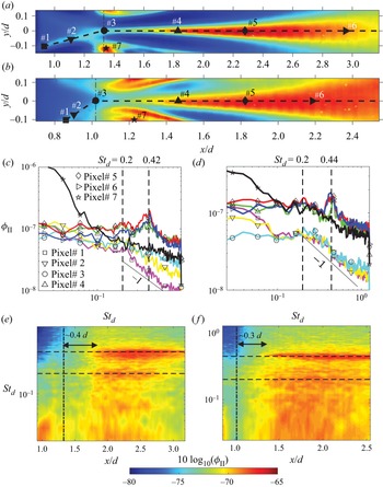
We now consider the dynamics of the cylinder wake through a Fourier analysis of the focussing schlieren light intensity fluctuations. The results will be presented in the form of the spectral density of horizontal knife-edge schlieren light intensity fluctuations that are proportional to the vertical density gradient fluctuations ( $\partial \rho '/\partial y$) in the wake. Figures 10(a) and 10(b) show the variance images from the horizontal knife-edge 100k near-wake dataset for the 12 mm and 15 mm cylinders, respectively. The power spectral density of the vertical density gradient fluctuations corresponding to the pixels# 1–7 marked on the variance images in figures 10(a) and 10(b) are presented in figures 10(c) and 10(d), respectively. The vertical line on each variance image marks the mean reattachment location (
 $x_r$) estimated in the previous section (see table 3). The shape of the symbols used to mark the pixel locations matches the symbols on the spectral lines. The frequency in the spectral plots has been normalised on the cylinder diameter and the incoming free-stream velocity to yield the Strouhal number,
 $St_d$. Unless otherwise stated, this non-dimensionalisation of frequency will be used throughout the text.
Power spectral density of light intensity fluctuations in the wake of the circular cylinders. (a,b) Show the pixel locations on the variance images for the 12 mm and 15 mm cylinders, respectively, for which the spectra are shown in (c,d); the legend for both is shown in (c). (e, f) Show contours of spectral density of light intensity fluctuations on log scale ( $10\log _{10}(\phi _{II})$) along the wake centreline for the 12 mm and 15 mm cylinders, respectively. The vertical line represents the approximate mean reattachment location (
 $x_r$) and the two horizontal lines represents the Strouhal numbers at which peaks are observed in the line spectra. The colour scale for the contour plots is the same and shown at the bottom.

First consider the spectrum measured at the foot of the trailing shock (represented by the  $\star$ symbol) for each cylinder. These spectra stand out from the rest of the spectra since the spectral magnitude at low frequencies (
 $St_d < 0.08$) for both the cylinders is significantly larger than the spectra elsewhere. Based on the free-stream velocity, the smallest length scales corresponding to these low-frequency oscillations are approximately 13.5
 $d$ and 12.9
 $d$ for the 12 mm and 15 mm cylinders, respectively. This large, low-frequency unsteadiness of the shock foot is reminiscent of the low-frequency unsteadiness observed in recompression shocks in a backward-facing step flow (Poggie & Smits Reference Poggie and Smits2001) as well as an axisymmetric wake (Simon et al. Reference Simon, Deck, Guillen, Sagaut and Merlen2007). In both cases, the large-scale unsteadiness points to a global oscillation of the recompression shock waves caused by the unsteadiness of the oncoming vortical structures in the shear layer. This also appears to be the case in the present work.
Now consider the spectra for the two points within the shear layer (represented by  $\square$ and
 $\triangledown$) and within the reattachment region (represented by
 ) for the 12 mm cylinder (figure 10c). The spectra here are broadband and do not show any clear peaks which may indicate the absence of any vortex shedding. The spectrum for the most upstream pixel selected in the image (
 $\square$) shows nearly a
 $-$1 roll-off with frequency for
 $St_d > 0.2$. As the shear layer approaches the reattachment point and undergoes compression, the roll-off slope becomes shallower, and the higher frequencies become more energetic. The presence of the
 $-$1 roll-off in the free shear layer is curious as it is typically associated with velocity spectra in both incompressible and compressible boundary layers (Smits Reference Smits1995). Garg & Settles (Reference Garg and Settles1998), who performed focussing schlieren deflectometry of a supersonic turbulent boundary layer, have shown that the shape of the spectrum obtained using a focussing schlieren set-up with horizontal knife-edge placement is nearly identical to the spectrum of voltage fluctuations from a hot-wire anemometer, and they both show a roll-off with
 $-$1 slope. They have argued that this equivalency is acceptable as long as strong Reynolds analogy is valid such that the density fluctuation, the mass-flux fluctuations, and the velocity fluctuations are all linearly related. Assuming this is also the case here, the result implies that
 $-1$ slope also exists in compressible free shear layers. The breakdown of the
 $-1$ slope and energisation of high-frequency fluctuations just upstream of the reattachment point (represented by
 ) suggests that the recompression process is responsible. This is consistent with the observations of Smith & Dutton (Reference Smith and Dutton1996), who studied the planar, supersonic free shear layer and its recompression/reattachment in base flow through Mie scattering, and found more diverse range of length scales in the recompression region than further upstream in the shear layer. Although the present flow is different from their study, the spectral behaviour in the present work also suggests that the recompression of shear layers in the adverse pressure gradient region near the reattachment point causes finer length scales in the shear layer to become energetic. The spectra for the 15 mm cylinder in the shear layer also show a similar behaviour except that the high-frequency fluctuations are not as energetic and it appears that the
 $-1$ slope region is extended to higher frequencies, which is consistent with the higher Reynolds number for this case.
Next, consider the spectra in the wake at the three different streamwise locations (represented by  $\triangle$,
 $\Diamond$ and
 $\vartriangleright$) along the wake centreline as shown in the variance images. Again, the qualitative behaviour of the spectra is similar for the two cylinders. Compared with the shear-layer spectra, the spectra in the wake show a different character with a near-flat shape for
 $St_d < 0.2$, and consistent with the results of Schmidt & Shepherd (Reference Schmidt and Shepherd2015), a clear peak near
 $St_d = 0.42\pm 0.02$ (
 $21.1\pm 1\ {\rm kHz}$) and
 $St_d = 0.44\pm 0.02$ (
 $17.5\pm 1\ {\rm kHz}$) can be observed for the 12 mm and 15 mm cylinders, respectively. The peaks are broadband in nature and do not occur at the same frequency across the wake, and so the uncertainty in the estimation of the peak frequency is approximately 1 kHz, which yields an uncertainty in the Strouhal number of approximately 0.02. These results confirm the finding of Schmidt & Shepherd (Reference Schmidt and Shepherd2015) that the periodicity in the wake of a circular cylinder placed in a supersonic flow occurs at a higher frequency than that observed if the same cylinder was placed in an incompressible flow.
The distribution of vertical density gradient fluctuations across different frequencies in the cylinder wake can be visualised in a more lucid manner in figures 10(e) and 10( f), which show the spectral density within the shear layer and the wake on a contour map for the 12 mm and 15 mm cylinders, respectively. Here, the spectral densities are plotted on a log scale ( $10\log _{10}(\phi _{II})$) as a function of streamwise distance and Strouhal number. The contour maps were created by extracting the spectral densities from each pixel along the dashed lines shown in the variance maps of figures 10(a) and 10(b), and then plotting them as a function of the streamwise location (
 $x/d$) of each pixel. The vertical line superimposed upon the contour map represents the mean reattachment location estimate. Both maps show a clear presence of the spectral peaks that become apparent slightly downstream (approximately at
 $x/d = 1.7$ and 1.4 for
 $d = 12\ {\rm mm}$ and 15 mm respectively) of where the wake originates. Interestingly, for the 12 mm cylinder, a clear second peak at
 $St_d = 0.2$ is also observed. This peak co-exists with the
 $St_d= 0.42$ peak until it dissipates near
 $x/d = 3$. Although masked by the intense fluctuations below the peak frequency for the 15 mm cylinder, a localised rise in spectral power near
 $St_d = 0.2$ can also be observed when individual line spectra such as those in figure 10(d) are analysed. This suggests that the canonical Kelvin–Helmholtz instability associated with incompressible flow over a cylinder that leads to vortex shedding in the wake may also exist in the early wake of a cylinder in supersonic flow, however, the compressibility serves to stabilise this instability. Note that throughout the rest of this paper, the term vortex shedding frequency or the peak frequency will refer only to the periodicity observed around
 $St_d = 0.4$ for both cylinders.
Besides the clear existence of the vortex shedding peaks, a few other observations can me made from the contour maps of spectral densities. Firstly, the peaks appear some distance downstream of the mean reattachment point (highlighted using the vertical dashed lines in the maps). Even if we account for the uncertainty in the estimation of the reattachment point (which is half the reattachment length,  $L_r/2$), it seems that the vortex shedding originates in the wake and not in the shear layers or within the reattachment region. It is, of course, possible that the vortex shedding strength further upstream is too weak to be picked up by the current imaging system. Regardless, this suggests that either the wake instability is convective in nature or some other mechanism (e.g. aeroacoustic resonance) is at play. Later in § 3.5 we provide evidence which supports the latter argument. Next, we note that the reattachment process energises the high-frequency fluctuations in the flow as evident in the disappearance of the blue patches towards the top left of the contour maps immediately after the mean reattachment location. Additionally, the reattachment process also appears to somewhat suppress the low-frequency oscillations as evident in the disappearance of the red patches towards the bottom-left corner of the contour maps. As the wake begins to develop, a broadband increase in the energy at frequencies below
 $St_d = 0.2$ is also observed for both the cylinders. This amplification is particularly intense for the 15 mm cylinder where it masks the
 $St_d = 0.2$ peak. This low-frequency energy enhancement post-reattachment decays rapidly as evident in the spectral map for the 12 mm cylinder. The fov of the 15 mm cylinder in the streamwise direction is not wide enough to capture the same phenomenon.
Before we move forward, a note on the scaling of the peak frequencies. The present Reynolds number difference between the two cylinders is not significant enough to confirm the scaling on the slipline length proposed by Schmidt & Shepherd (Reference Schmidt and Shepherd2015). Moreover, it is not clear where the sliplines lie within the shear layer in the present work. However, if we take the shear-layer length ( $L_s$; see table 3) as a proxy for the slipline length, then scaling the peak frequency on
 $L_s$ yields Strouhal numbers of approximately 0.51 and 0.41 for
 $d = 12\ {\rm mm}$ and 15 mm, respectively. These Strouhal numbers do not appear to converge, but they do lie between 0.4 and 0.6, which is the range of the slipline-based Strouhal numbers reported by Schmidt & Shepherd (Reference Schmidt and Shepherd2015). Another possible choice of the length scale is the length of the reattachment region (
 $L_r$), which implies that the disturbances being propagated into the wake are a result of the unsteadiness of the reattachment process. Scaling the frequencies on
 $L_r$ yields a Strouhal numbers of 0.16 and 0.14 for the 12 mm and 15 mm cylinders, respectively. This convergence is better than on
 $L_s$. The scaling on reattachment length does have a physical basis as well when one considers that the streamwise pulsation of the reattachment region has been shown to be the dominant global feature of planar wakes in the high supersonic Mach number range (Scarano & Oudheusden Reference Scarano and Oudheusden2003; Humble et al. Reference Humble, Scarano and van Oudheusden2007).
3.3. Standing waves in the cylinder wake
We will now show that the supersonic cylinder wake consists of a standing wave pattern which hints at the presence of aeroacoustic resonance in the early wake. The results will also show that the onset of the vortex shedding around  $St_d = 0.4$ for the cylinders is accompanied by the strengthening of the standing wave pattern which implies a relationship between the two. Note that the term standing wave here refers to the result of an interference between upstream/downstream propagating instabilities which can be visualised by considering the spatio-temporal correlation between the disturbances in the wake. To visualise these standing waves we will utilise the frequency-domain coherence between density gradient fluctuations at different pixel locations. The coherence function (
 $\gamma$) is defined as
 \begin{equation} \gamma^2(f) = \frac{|S_{ij}(f)|^2}{\phi_{ii}(f)\phi_{jj}(f)}, \end{equation}
where,  $S_{ij}$ is the cross-spectral density between schlieren light intensity fluctuations for any two pixels
 $i$ and
 $j$, and
 $\phi _{ii}$ and
 $\phi _{jj}$ are the auto-spectral densities of the light intensity fluctuations for
 $i$ and
 $j$, respectively. Figure 11(a) shows the variance image for the 12 mm cylinder from 100k near-wake dataset with the three dashed lines representing trajectories along which the coherence function will be presented. The solid markers along each of these trajectories show the location of the reference pixel (pixel
 $i$) with respect to which the coherence function was calculated. In each case, the coherence between the reference pixel and the remaining pixels along the trajectory (pixel
 $j$) was calculated. The inclined dashed line represents the shear-layer trajectory up to the mean reattachment location, while the lower and the upper horizontal dashed lines lie in the wake at
 $y/d = 0$ and 0.07, respectively. The coherence will be plotted as a function of both the frequency and the spatial coordinate of pixel
 $j$. The spatial coordinate system for the reference points along the two horizontal trajectories is such that
 $\Delta x$ = 0 represents the reference pixel location and positive
 $\Delta x$ runs in the downstream direction. The spatial coordinate (
 $\Delta \eta$) for the shear layer trajectory (inclined dashed line in figure 11a) is defined such that
 $\Delta \eta = 0$ is located at the reference point# 1 and positive
 $\eta$ runs downstream up to the mean reattachment location. The three reference points along the wake centreline trajectory lie at
 $x/d = 1.02$, 1.28, and 1.72, while the coordinates of point# 5 are
 $(x/d, y/d) = (1.72, 0.07)$. Note that point# 2 and point# 3 are located within the recirculation and the reattachment regions, respectively, while point# 4 is located approximately where the vortex shedding at
 $St_d = 0.42$ first becomes noticeable. In the case of shear layer, the coherence between the reference point and every fifth pixel downstream of it was calculated, whereas in the wake the data from every tenth pixel was utilised. To minimise ambiguity in the two-point statistics due to noise, only coherence values greater than 10 % (
 $\gamma ^2 > 0.1$) will be shown.
Coherence between the reference points highlighted on the variance image in (a) using  $\bullet$ and the rest of the pixels along the trajectories denoted by dashed lines. Coherence with points# 1, 2, 3, 4 and 5 as reference locations are shown in (b), (c), (d), (e) and ( f), respectively. The coherence function calculated from the conventional schlieren dataset with the reference point placed at the same location as point# 4 is shown in (g). The coherence values shown are restricted between 0.1 and 0.8 and the colour bar for each contour map is shown at the bottom.

Now consider figure 11(b–f) which shows the coherence function for each reference pixel as a function of both space and time. The coherence function within the shear layer (figure 11b) has a different appearance than those within the wake and it shows typical turbulent shear flow behaviour with larger correlation lengths at lower frequencies. Although not apparent in the contour map, at a given frequency, the coherence decays with a near-exponential rate with increasing streamwise separation, also a familiar trait of shear flows. The appearance of coherence maps here, along with the presence of  $-$1 slope in the shear-layer schlieren spectra previously shown in figure 10(c,d) suggests that focussing schlieren data may be useful in extracting a spanwise-averaged measure of turbulence statistics, even in flows with strong end effects. Note that the coherent length scale within the shear layer also shows a slight increase between
 $St_d = 0.2$ and
 $St_d = 0.3$ (marked by the localised ridge in the coherence map near these frequencies) which could be an indication of the presence of the canonical K–H instability within the shear layer. Presumably, this instability grows during the wake formation leading to a peak near
 $St_d = 0.2$ in the early wake, however, it then decays rapidly as the wake accelerates and compressibility increases. The suppression of the instability with increasing Mach number in the wake is perhaps not surprising given that compressibility is known to curb the instability growth rates in shear layers (Papamoschou & Roshko Reference Papamoschou and Roshko2006).
Now consider the coherence maps for the three reference points along the wake centreline (points# 2–4). The coherence with respect to point# 2 which is located within the recirculation region (figure 11c) has a similar appearance as that in the shear layer with large correlation lengths at lower frequencies, however, it does not show a localised peak around  $St_d = 0.2$. The coherence here also shows the presence of a weakly coherent disturbance near the peak frequency (
 $St_d = 0.42$) for
 $\Delta x/d >0.8$, suggesting a link between the vortex shedding in the wake and the disturbances within the recirculation region. Further downstream, with reference points placed at the mean reattachment location and within the wake (points# 3 and 4, figure 11d,e), the disturbances near the peak frequency become more coherent and discrete, coherent bands along the frequency axis which appear to be centred at sub-harmonics of the peak frequency appear. Interestingly, a banding of the coherence function is also observed along the spatial axis, implying the presence of spatial harmonics in the early wake. The spatial harmonics are broadband in time and have a characteristic length scale of approximately 0.35
 $d$, regardless of the frequency. These spatial harmonics point to the presence of standing waves in the wake which may form as a result of aeroacoustic resonance. It is also interesting to note that this spatial resonance is limited to the wake region since the coherence map with reference point placed outside the wake (point# 5, figure 11f) does not show any banding in the spatial direction. However, the region outside the wake does show temporal resonance (banding along the frequency axis) which suggests that the disturbance waves with the same frequency are present inside and outside the wake, but they only lead to spatial resonance in the wake. As explained later in § 3.5, the reason for this is that, unlike the region outside the wake, the wake is subsonic and supports both upstream and downstream propagating waves which interact with each other to create standing waves within the wake.
The spatio-temporal resonance observed in the coherence maps here has not been noted before for cylinder wakes and it is entirely possible that this is also a general feature of planar supersonic wakes where strong acoustic waves may exist. Standing waves in supersonic flows, however, do exist in both screeching supersonic jets (Panda Reference Panda1999) and supersonic impinging jets (Bogey & Gojon Reference Bogey and Gojon2017) where they are known to be caused by an interaction between hydrodynamic instabilities and upstream propagating acoustic waves. However, in these cases the upstream propagation is a result of the presence of a discontinuity (shock cells in jets and the wall in impinging jets), whereas in the present case no such features are present to provide an influx of acoustic energy. However, as discussed later in § 3.5, there is evidence that in the present work the wake receives the acoustic energy input through acoustic waves that are generated from the unsteady shear-layer separation on the cylinder surface. Finally, we note that the coherence obtained from the conventional schlieren images (figure 11g) with reference point the same as point# 4 in the focussing schlieren maps is similar in appearance, and although weaker, it also shows coherent banding along both spatial and temporal dimensions. This suggests that statistics obtained using conventional schlieren in bluff supersonic wakes can be meaningful due to the features in the two-dimensional region, rather than the three-dimensional end regions, dominating the path integration of light deviations. Note that the conventional schlieren coherence map only shows the second spatial harmonic at  $\Delta x/d = 0.7$ which could be due to a lower sampling rate (60 000 fps) or a difference in the range and sensitivity of the imaging systems.
To further understand the spatio-temporal resonance in the cylinder wake, we will now present the coherence function plotted in two different manners. First, we calculate the coherence function between a reference pixel along the wake centreline and the rest of the pixels in the schlieren image at a given frequency as shown in figure 12(a–c). The coherence images in (a,b) were calculated from the 12 mm cylinder 100k near-wake dataset at  $St_d = 0.2$ and 0.42, respectively, with the reference pixel located at
 $x/d = 1.7$ in each case. The image in (c) was calculated at
 $St_d = 0.42$ with reference pixel at
 $x/d = 2.0$ from the 12 mm cylinder 50k near-wake dataset. The edges depicting the boundaries of the salient wake flow features calculated previously in § 3.1 have been superimposed upon the coherence images for spatial reference. The images have been stretched in the
 $y$ direction by a factor of 2 in order to show the features clearly.
Standing waves in the 12 mm cylinder wake revealed through the coherence function. The coherence between a reference pixel (marked using  $\times$) along the wake centreline and remaining pixels in the image is shown in (a–c). The images in (a,b) show the coherence at
 $St_d = 0.2$ and 0.42, respectively, calculated using the 100k near-wake dataset, while the image in (c) was extracted from the 50k near-wake dataset. The spatial distribution of the standing waves along the wake centreline is shown in (d–f). These images were obtained by shifting the reference point (denoted by coordinate
 $x_1$) to every tenth pixel along the centreline and then plotting the coherence between the reference point and the remaining pixels along the centreline. (d,e) Show the coherence along the centreline for the 12 mm cylinder at
 $St_d = 0.2$ and 0.42, respectively, while ( f) shows the coherence at
 $St_d = 0.44$ for the 15 mm cylinder.

Considering the coherence images in figures 12(a) and 12(b) we note that the coherence function plotted in this manner clearly reveals the standing waves in the wake which manifest as discrete coherent spots spaced apart by 0.35 $d$. These plots also show that the standing waves are more intense at the peak frequency than at
 $St_d = 0.2$. If we now consider the coherence image at the peak frequency in figure 12(c) which is same as (b), but has a larger fov in the vertical direction, several interesting aspects can be noted. First, this image clearly shows that the standing waves do not appear outside the wake where the flow is supersonic, bolstering the hypothesis that the spatial coherence is likely a result of an interaction between the upstream/downstream propagating waves. Additionally, this image also shows that the recompression waves oscillate coherently with the wake. It will be shown in § 3.4 that this coherent oscillation is a result of a ripple type of shock motion caused by compression waves radiating from the coherent wake structures. We also note that the wavelength associated with the coherent spots in the 50k near-wake dataset in (c) is twice that observed in the 100k near-wake dataset in (a,b). This is similar to what was observed with the conventional schlieren dataset in figure 11( g) and may be attributed to spatial aliasing in the 50 kHz dataset or differences in the imaging systems.
The second manner in which the coherence function is plotted is shown in figure 12(d–f) where only the 100k near-wake dataset is used to reveal the spatial distribution of the harmonics along the wake centreline. Here, figure 12(d,e) plots the coherence for the 12 mm cylinder at  $St_d = 0.2$ and 0.42, respectively, while figure 12( f) plots the coherence for the 15 mm cylinder at
 $St_d = 0.44$. To create these plots, the reference point (designated as
 $x_1$) was shifted to every tenth pixel along the centreline and its coherence with the rest of the pixels along the wake centreline was calculated. Next, the coherence values at each frequency were plotted as a function of both
 $x_1$ (reference points) and
 $x$ (the remaining pixels) as filled contours. The two vertical dashed lines in each plot show the approximate streamwise locations of the reattachment point (
 $x_r$) and the location where the vortex shedding peak is first noticed in the schlieren pixel intensity spectra (
 $x_{sh}$). Naturally, plotting the coherence in this way yields a value of 1 for
 $x_1 = x$, hence the thick red strip inclined at
 $45^\circ$. The coherent strips to the right and left of this strip are the spatial harmonics upstream and downstream of the reference pixel (
 $x_1$), respectively. Considering the plots for the 12 mm cylinder in figure 12(d,e), it is clear that the peak frequency in (e) is associated with stronger spatial harmonics in the wake and the resonance begins to develop almost immediately after the reattachment point (
 $x_r$), but it is not present in the recirculation region (or is too week to observe). Between the mean reattachment location and where the vortex shedding first becomes apparent in the schlieren intensity spectra (
 $x_r < x_1 < x_{sh}$), spatial harmonics are only observed in the downstream direction, but the appearance of the peak in the schlieren intensity spectra near
 $x_{sh}$ is accompanied by harmonics in both directions. The strengthening of the coherent resonant peaks near the location where the vortex shedding is first observed suggests that the vortex shedding in the cylinder wake may simply be a result of aeroacoustic resonance. Note that this conclusion itself is not different from that reached by Schmidt & Shepherd (Reference Schmidt and Shepherd2015) based on scaling arguments, except that in § 3.5 we show that the resonance is primarily linked to the acoustic disturbances outside the approaching shear layers where the flow is supersonic, rather than those within the recirculation region. Finally, we note that the spatial harmonics are also observed for the 15 mm cylinder (figure 12f), but it shows fewer side lobes than the 12 mm cylinder and its presence in the reattachment region cannot be clearly verified. The reason for these differences is twofold – a limited fov and inadequate sensitivity/range of the imaging system for this case since the system was tuned for visualising the 12 mm cylinder wake.
The implicit assumption behind the hypothesis proposed here that the standing waves are a result of an interaction between upstream/downstream propagating instabilities is that the early portion of the redeveloping wake contains a subsonic portion that supports upstream propagating disturbances. To verify this assumption the mean flow field around the 12 mm cylinder was calculated using a two-dimensional compressible Reynolds-averaged Navier–Stokes (RANS) solution that will now be briefly discussed. The solution was carried out on a rectangular domain with the same height as the wind tunnel (142.6 mm) and a length of 142 mm (12 $d$) in the streamwise direction. The cylinder was placed at the centre height of the domain,
 $2d$ downstream of the domain inlet. The domain was meshed using the ANSYS meshing software with a target sizing set on the free-stream region and an inflation-type mesh around the cylinder surface to better resolve the shear layer. Four different mesh sizes of 36 883, 130 777, 428 800 and 744 508 elements were used to verify the grid independence of the final solution. A far-field pressure-type boundary condition was specified at the domain inlet with a total pressure of 600 kPa and a temperature of 105 K, while the domain outlet was set to be a pressure outlet. The upper and lower walls and the cylinder surface were set to stationary walls with a no-slip boundary condition. A steady, density-based solver in ANSYS Fluent with the two-equation
 $k{-}\omega$ shear stress transport model for the viscous terms was used to calculate the flow field around the cylinder. A first-order upwind discretisation scheme was used for the flow parameters, while the turbulent quantities were calculated using a second-order upwind method using the advection upstream splitting method scheme. The Courant number was set to 10 and the convergence criterion was set to
 $2(10^{-5})$ for all residual properties. The Reynolds number of the simulations is
 $Re_d = 5.5(10^5)$ which is of the same order as the Reynolds number in the measurements (
 $Re_d = 6.0(10^5)$).
Figure 13 shows the global flow field calculated using the RANS solution in form of a filled contour map of local Mach number. The dashed lines in the plot represent the sonic lines in the flow and the solid lines are the edges that were calculated from the schlieren images for the 12 mm cylinder. Figure 13 inset shows an enhanced view of the Mach number distribution over the same fov as the focussing schlieren system. These results show that the flow along the wake centreline is indeed subsonic in the early part of the redeveloping wake up to a certain distance downstream of the cylinder centre and therefore can support both upstream and downstream propagating modes. To further understand the flow features which may be responsible for the standing waves observed in this section, we now present coherent structures in the wake obtained through POD of density gradient fluctuations contained in the schlieren datasets.
Mach number distribution around the 12 mm cylinder estimated using a two-dimensional, steady compressible RANS solution with dashed lines representing sonic lines in the flow. The edges for the 12 mm cylinder calculated from the schlieren images have been superimposed as solid lines for comparison. The inset shows an enhanced view of the Mach number distribution behind the cylinder with the same fov as the 50k near-wake schlieren dataset in the experiments.

3.4. Coherent structures in the cylinder wake
In this section we reveal coherent oscillations in the wake of the cylinder through POD of schlieren light intensity fluctuations that have been bandpass filtered in time around specific frequencies. Figures 14(a) and 14(b) show the magnitude and the phase response, respectively of the finite impulse response (FIR) bandpass filter which was applied to the schlieren light intensity fluctuation ( $I'(t)$) in each pixel. The filter has a passband bandwidth of 2 kHz with a centre frequency of 21 kHz (
 $St_d = 0.42$) and a stopband attenuation of 85 dB with a steepness slope of 0.85. The phase of the filter as shown in (b) is linear in the passband frequency range such that there is no phase distortion. The same filter, but with its centre frequency shifted to
 $St_d = 0.2$, 0.3 and 0.7, was applied to the schlieren datasets to differentiate the wake behaviour at these frequencies from that at the peak frequency. From here on the results from POD of the bandpass-filtered schlieren images will be referred to by specifying the centre frequency of the bandpass filter applied to the dataset. Note that a total of
 $2^{12}$ schlieren images were filtered and used for the averaged statistics presented in this section.
Bandpass filtering and conditional averaging to isolate frequency components in the schlieren images. (a,b) Show the magnitude and phase response of the FIR bandpass filter, respectively.

Figure 15 shows the POD eigenvalues (first row) and the four most energetic spatial modes (POD eigenvectors) at  $St_d = 0.2$ (a,d,g,j,m), 0.3 (b,e,h,k,n) and 0.42 (c, f,i,l,o). The eigenvalues have been normalised such that their sum is unity so that the fractional contribution of each mode to the overall energy in the dataset can be evaluated. Only the leading 20 eigenvalues are shown which together account for approximately 56.8 %, 56.4 % and 66.6 % of the total energy in the dataset for
 $St_d = 0.2$, 0.3 and 0.42, respectively. The edges obtained from the variance image have been superimposed upon each mode for spatial reference. Each filtered POD mode has been stretched by a factor of two in the vertical direction in order to show the features clearly and the percentage contribution of each spatial mode to the total energy in the dataset is listed to the north west of that mode. Throughout the remaining paper, we will follow this same format to present POD modes, filtered or otherwise. First consider the POD eigenvalues shown in (a–c) for the three frequencies. The most energetic POD modes at
 $St_d = 0.2$ and 0.3 contribute around 10 % to the overall energy, whereas at
 $St_d = 0.42$ this contribution is nearly doubled and the two leading modes account for nearly 30 % of the total energy in this case. At
 $St_d = 0.2$ and 0.3 this contribution drops to 18.8 % and 16.6 %, respectively. These values suggest that the POD of the focussing schlieren datasets can successfully extract dominant dynamics in the cylinder wake.
The leading 20 POD eigenvalues (a–c) and the four leading eigenmodes (d–o) from bandpass-filtered schlieren images of the 12 mm cylinder wake. The first, second and third columns correspond to the bandpass-filtered images centred at  $St_d = 0.2$, 0.3 and 0.42, respectively. The first, second, third and fourth most energetic modes for each frequency are shown in the second, third, fourth and fifth rows, respectively. The individual energy contribution of each mode is listed to the north west of that mode. The eigenvectors within each mode have been scaled between
 $-$0.5 and 0.5 and the colour scale is shown at the bottom of the plot.

Now consider the two leading POD modes for the three frequencies as shown in figure 15(d–i). The two modes at each frequency have a similar appearance and show coherent structures being generated in the wake as well as along the recompression wave which bounds the wake on either side. At each frequency, the two modes show similar coherent structures that appear to be translated. As discussed later, this is because these are what are referred to as coupled POD modes and they show the same phenomenon with a spatial phase shift. The spatial coherence within the shear layer and in the reattachment region is weaker than in the wake for each mode shown here. The weaker spatial coherence in this region could be an indication of the presence of three-dimensional instabilities which have previously been shown to exist in the recompression region of compressible shear layers (Smith & Dutton Reference Smith and Dutton1996). The presence of three-dimensional instabilities leads to a degeneration of spanwise organisation of turbulent structures (Clemens & Mungal Reference Clemens and Mungal1992) which could affect POD results since they rely on spatial coherence. Note that the opposite sign on the eigenvectors (red and blue colours) of similar appearance within a mode may be interpreted as a sign of convected structures (Weiss Reference Weiss2019). The coherent structures at  $St_d = 0.42$ ( f,i) have a smoother appearance due to larger energy contained within these modes. Nonetheless, the two leading modes show that the wake consists of large, coherent structures which span the entire wake width and whose streamwise length scale may exceed the cylinder diameter (the former fact also being a testament to the accuracy of the edge-detection algorithm discussed earlier). Regardless of the frequency, the wake structures are elongated in the streamwise direction and are reminiscent of the results of Humble et al. (Reference Humble, Scarano and van Oudheusden2007), who have shown the existence of similar elongated structures in a planar supersonic wake at
 $M = 2.27$. They have attributed the shape of these structures to the streamwise pulsation of the reattachment region, rather than a flapping-type motion observed at lower supersonic Mach numbers. This streamwise-aligned motion of the reattachment region is quite possibly related to a change in the stability characteristics of the oncoming shear layer as well as its interaction with the recirculation region behind the cylinder. It is also noteworthy that the elongated shape of the coherent structures in the wake is also markedly different that those found in POD modes of an incompressible wake of a cylinder (Ma, Karamanos & Karniadakis Reference Ma, Karamanos and Karniadakis2000) where they tend to be stretched in the vertical direction. This could suggest that, similar to a planar supersonic wake, the cylinder wake instability is of varicose (symmetric) type, rather than sinuous (anti-symmetric) type observed at lower Mach numbers.
Besides the coherent wake structures, another noteworthy aspect of the leading POD modes in figure 15(d–i) is the presence of coherent oscillations near the recompression wave seen towards the top and bottom edges of the images, beginning around  $x/d = 2$. These oscillations are symmetric in nature, implied by the same sign of the eigenvector associated with them. At the peak frequency, these symmetric oscillations appear to be linked to weak compression waves radiating from the leading edge of the coherent wake structures. A closer observation of the second mode at
 $St_d = 0.42$ in figure 15(i) reveals that these compression waves form in the reattachment region and they perturb the recompression waves as they convect downstream. These compression waves are most likely weak eddy shocklets which have been observed in both supersonic flat-plate wake (Clemens & Smith Reference Clemens and Smith1998) and mixing layers (Smith & Dutton Reference Smith and Dutton1995). The symmetric, coherent disturbances along the recompression waves also appear in the two leading modes at frequencies lower than the peak frequency (figure 15d,e,g,h) with the size of the structures increasing as the frequency decreases. However, no evidence of shocklets is observed at these frequencies. Instead, it appears that that at these frequencies the shocks generate disturbances which propagate towards the wake centreline (this is most clearly observed in the second mode at
 $St_d = 0.2$ in figure 15g). Lastly, it is worth noting that the horizontal knife-edge schlieren pixel intensities from which the POD modes are extracted are anti-symmetric about the image centreline (same structures on either side appear opposite in light intensity) which will produce POD eigenvectors of the same sign if these structures move in the same direction relative to the image centreline and vice versa. This anti-symmetry, however, may not affect the symmetric or anti-symmetric nature of coherent structures implied by the POD eigenvectors. It is possible that the symmetry implied by the POD eigenvectors are generated by symmetric light intensity fluctuations (opposing structures on either side with similar intensity magnitude). Further, note that POD calculation relies on the covariance between the schlieren pixel intensity fluctuations and the sign of the eigenvectors are indicative of the correlation (same sign) or anti-correlation (opposite sign) between these fluctuations, rather than the absolute value of the pixel intensity.
To shed further light into the oscillations of the recompression wave, figure 16(a–c) shows the leading POD mode at  $St_d = 0.2$, 0.3 and 0.42 obtained by the decomposition of the filtered 50k upper-wake dataset (see table 2 in § 2.2). Recall that this dataset only shows the upper half of the wake such that the dynamics of the recompression wave can be clearly observed. The decomposition of this dataset at the peak frequency (figure 16c) reveals that the shocklet-generated disturbances remain attached to the wake structures and they perturb the recompression wave as the eddies convect downstream, essentially causing the recompression wave to ripple. The leading modes at
 $St_d = 0.2$ and 0.3 (figure 16a,b) also show signs of this ripple-type motion, however, the shocklets are not observed at these frequencies.
The first (a–c) and third (d–f) POD modes of the 50k upper-wake dataset for the 12 mm cylinder filtered at  $St_d = 0.2$ (a,c),
 $St_d = 0.3$ (b,e) and
 $St_d = 0.42$ (c, f).

We now go back to figure 15(j–o) to analyse the lower-order POD modes of the filtered datasets which, like the leading modes, are coupled and show the same flow feature with a spatial phase shift. Although these modes are less energetic, it will be shown in the next section that they are responsible for the aeroacoustic resonance which leads to the formation of standing waves in the wake. Firstly, we note that, regardless of the frequency, the dominant dynamics within these modes is that of coherent disturbances located near the recompression waves. Secondly, unlike the ripple-type motion observed in the leading POD modes, these oscillations are anti-symmetric above the wake axis, as indicated by the opposite sign on the eigenvector. These disturbances are also broadband, as indicated by their similar appearance at each frequency and they can perturb the wake, particularly at the peak frequency as observed in figure 15(l). At first glance, it may seem that these oscillations may represent an alternating movement of the recompression waves. However, if we consider the third modes from the 50k upper-wake dataset shown in figure 16(d–f), we can see that the origin of these oscillations is upstream of the recompression wave. It appears that these anti-symmetric disturbances are waves which originate upstream of the recompression wave and are then amplified by the latter. Also note that no such waves are present upstream of the symmetric oscillations represented by the leading modes in figure 16(a–c).
To further understand the coherent structures in the cylinder wake, we consider the filtered POD modes from conventional schlieren as shown in figure 17. These plots show the first and the third modes at the same three frequencies ( $St_d = 0.2$, 0.3 and 0.42) for which the focussing schlieren POD modes were considered. Despite contamination of the density gradients by the three-dimensional sidewall flow, these images are useful to understand the global behaviour of the cylinder wake due to their large fov. Regardless of the frequency, both the modes shown here have less fractional energy than the corresponding modes from focussing schlieren datasets in figure 15. However, the leading modes still show statistically significant contributions and confirm the presence of shocklets and the ripple-type motion of the recompression shock, most clearly observed at the shedding frequency in figure 17(c). It is, however, the third mode from conventional schlieren which is of interest here. This mode clarifies that the anti-symmetric oscillations near the recompression wave observed in the third/fourth mode of the filtered focussing schlieren datasets are, in fact, acoustic waves which appear to be originating upstream of the recompression wave. The speculation that these are acoustic waves is bolstered by the fact that the coherent length scale of these disturbances is much greater than any characteristic length scale of the flow and that they are oriented at an angle to the local flow direction. The convective velocity of these disturbances in the wake (estimated using the wavelength extracted from the POD mode) is approximately
 $260\ {\rm m}\ {\rm s}^{-1}$ which, assuming this is the local speed of sound, translates to a temperature ratio of 0.56 and
 $M = 2$. The Mach angle corresponding to
 $M = 2$ is
 $30^\circ$ and the angle of these waves estimated from the POD mode is in the range
 $30^\circ \unicode{x2013}33^\circ$, suggesting that these are, in fact, acoustic waves. Although not visible in the current results due to a limited fov, these waves likely originate from the separation point on the cylinder surface. In fact, these acoustic waves can also be observed in the raw vertical knife-edge focussing schlieren instantaneous images which were previously shown in figure 6(c, d). Through Euler computations of a Mach 4 cylinder wake, Schmidt & Shepherd (Reference Schmidt and Shepherd2015) have reported oscillations between the separation points on the cylinder surface and the end of the sliplines which converge at the neck behind the cylinder. It is possible that the acoustic waves observed here are the source of these oscillations, and, as shown momentarily, it is these acoustic waves which provide the acoustic energy input required for the aeroacoustic resonance to develop within the wake.
The first (a–c) and third (d–f) POD modes of the conventional schlieren dataset for the 12 mm cylinder at  $St_d = 0.2$ (a,c),
 $St_d = 0.3$ (b,e) and
 $St_d = 0.42$ (c, f).

The importance of the acoustic waves observed in the lower-order POD modes of the filtered schlieren datasets is further highlighted in figure 18, which shows the leading four POD modes of the unfiltered, broadband 50k near-wake dataset for the 12 mm cylinder along with the power spectral density of the POD temporal coefficients ( $a_i$ in (2.1); see § 2.4) associated with each mode. The POD mode themselves are a time-averaged representation of the most dominant features in the flow field; however, the temporal coefficient spectra (figure 18e) reveal the most energetic frequencies associated with each representation. The first broadband POD mode shows the convective wake structures and the ripples along the recompression shocks. Since these convective features are the most intense around
 $St_d = 0.2$ and 0.42, the temporal coefficient spectra show two clear peaks. The second mode shows structures which appear similar to the leading POD mode at
 $St_d = 0.42$ (figure 15f) and hence the spectra only show a clear peak around
 $St_d = 0.42$. The third mode which represents the acoustic disturbances has a broadband temporal coefficient spectra whose magnitude at frequencies below approximately
 $St_d = 0.1$ is of the same order as the spectra corresponding to the leading mode, which shows that these acoustic waves carry significant energy. The fourth mode shows similar acoustic waves as the third mode, however, now its temporal coefficient spectrum shows a steep rise in energy levels around the peak frequency. This is an interesting result because it suggests that the acoustic waves which become apparent in the lower-order modes are related to the vortex shedding observed in the wake. This observation is the motivation for the wavenumber analysis presented in the following section to reveal the mechanism behind the aeroacoustic resonance that occurs in the wake of the cylinder.
POD of the unfiltered, broadband focussing schlieren dataset for the 12 mm cylinder wake. The four most energetic modes in order of decreasing energy are shown in (a–d), while (e) shows the Fourier spectra of the POD temporal coefficient associated with the four modes.

3.5. Aeroacoustic resonance in the cylinder wake
We now undertake a wavenumber analysis of the filtered POD modes to reveal the mechanism behind the aeroacoustic resonance in the cylinder wake. Earlier in our discussion of the filtered POD modes we saw that certain modes occur in pairs and show the same flow feature, just shifted in space. Recently, these coupled POD modes have been exploited to reveal the interaction between upstream and downstream travelling disturbances in supersonic screeching jets (Edgington-Mitchell et al. Reference Edgington-Mitchell, Jaunet, Jordan, Towne, Soria and Honnery2018, Reference Edgington-Mitchell, Wang, Nogueira, Schmidt, Jaunet, Duke, Jordan and Towne2021). This interaction is already known to be linked to the formation of standing waves in these jets (Panda Reference Panda1999) and here we show that a similar interaction exists in a cylinder wake leading to the formation of standing waves revealed through the coherence function in § 3.3. To reveal the directionality associated with the coherent disturbances contained within the coupled POD modes we combine them into a complex signal and perform a wavenumber decomposition of this signal along the streamwise direction. This decomposition is written as
 \begin{equation} \boldsymbol{W}(\kappa_x,x,y) = \sum_{x} (\boldsymbol{\psi}_{Lg}(x,y)+{\rm i}\boldsymbol{\psi}_{Le}(x,y))\exp({-{\rm i}\kappa_xx}), \end{equation}
where  $\boldsymbol{\psi}_{Le}$ and
 $\boldsymbol{\psi}_{Lg}$ are the coupled POD eigenvectors which represent the same flow feature, but are in quadrature. We also make the distinction between the real and imaginary parts of the combined mode such that
 $\boldsymbol{\psi} _{Lg}$ and
 $\boldsymbol{\psi} _{Le}$ are the POD eigenvectors that represent the lagging and the leading waveforms, respectively. This distinction ensures that disturbances with positive and negative phase velocities are represented by
 $\kappa _x > 0$ and
 $\kappa _x < 0$, respectively. The coupled POD modes with similar energy levels do not always occur in any particular order of leading/lagging disturbance and so they were determined by inspecting the eigenvector waveform of the two coupled modes along the wake centreline. It must also be noted that a negative phase velocity (
 $\kappa _x < 0$) obtained by the analysis here does not necessarily mean that a disturbance is travelling upstream since its group velocity (the wave envelope) can still be positive. However, the disturbances at negative wavenumbers, if present, are indicative of wavepackets whose crests and troughs propagate upstream. Throughout the remaining text, we will refer to disturbances with positive and negative wavenumbers as downstream and upstream travelling disturbances, respectively, regardless of the propagation direction of the wave envelope.
Before we consider the wavenumber decomposition of the coupled POD modes, we first need to ascertain which POD modes of the filtered dataset are in quadrature. As an example, consider the leading four POD modes of the dataset filtered at the peak frequency for the 12 mm cylinder that were previously shown in figure 15( f,i,l,o). A visual inspection of these modes and comparable amounts of energy in them suggests that the first/second mode form one pair, while the third/fourth mode form another. The relationship between these modes can be further established by considering the phase portrait of different combination of these modes as shown in figure 19(a–d). The phase portrait is formed by plotting the POD temporal coefficients associated with two modes against each other. The POD temporal coefficients ( $a_i(t)$, see (2.1)) for any given mode are obtained by projecting the data matrix of schlieren light intensity fluctuations at every time instance on the POD eigenvector corresponding to that mode. It can be clearly seen that there is good correlation between the first/second mode pair (figure 19a) and the third/fourth mode pair (figure 19d) as implied by the near circular phase portrait (barring a few outliers likely due to measurement noise), while the other mode combinations produce an oval distribution. Thus, the first/second and third/fourth mode pairs represent the same flow feature with a spatial phase shift between them.
Wavenumber decomposition of the POD modes of the bandpass-filtered focussing schlieren datasets. (a–d) Show the phase portrait of four different pairs of POD modes of the schlieren dataset filtered at  $St_d = 0.42$ for 12 mm cylinder. The wavenumber decomposition of the first/second and third/fourth POD mode pairs are shown in the second and third rows, respectively for (e,i)
 $St_d = 0.2$; ( f,j) 0.3; (g,k) 0.42; (h,l) 0.7. The plots in (h,l) are extracted from the 100k near-wake dataset, hence the limited fov in the vertical direction.

Now consider the wavenumber decomposition of the first/second mode pair and third/fourth mode pair as shown in the second and third rows, respectively of figure 19. The decomposition is shown for four different frequencies with those at the highest frequency (figure 19h,l) calculated from the 100k near-wake dataset, while the rest are computed from the lower frame-rate 50k near-wake dataset. The contour maps here show the absolute value of the Fourier transform along the streamwise direction normalised on the maximum value found within each map on a log scale. The contour scale has been restricted to 10 dB down from the maximum within each map to show the dominant features clearly. The Fourier transform was calculated by zero padding the complex eigenvector at each  $y$ station to improve the wavenumber resolution from
 $\Delta \kappa _x/d = 0.43$ to
 $\Delta \kappa _x/d = 0.22$. We have checked to ensure that the zero padding only smooths out the wavenumber plots and does not alter the wavenumbers associated with the dominant features shown in these plots. The wavenumber shown here has units of
 ${\rm m}^{-1}$. The wavenumber corresponding to the salient features have been shown with an arrow on top of each plot.
The decomposition of the leading mode pair at each frequency (e–h) shows a vertical band of high energy at positive streamwise wavenumbers since this mode pair is dominated by the downstream convecting flow structures as evident in the POD modes from which these transforms were calculated (figure 15d–i). The wavenumbers at which these convective peaks are centred increases as the frequency increases. Some disturbances with negative phase velocity ( $\kappa _x < 0$) are also visible in these wavenumber maps as well, particularly near the top/bottom edges of the plots. These could be related to the unsteadiness of the recompression wave which causes it to oscillate back and forth. If we now consider the wavenumber transform of the third/fourth POD mode pair (figure 19i–l), we note that it consists of similar convective bands (
 $\kappa _x > 0$) of energy as the leading mode transform, however, they are not as well defined except at the peak frequency. Of interest here, however, are disturbances in the negative wavenumber space which imply the presence of upstream propagating disturbances. With the exception of the mode at
 $St_d = 0.2$, a clear contribution at negative wavenumbers can be observed around
 $y/d = 0$ at each frequency. This contribution is particularly well defined in the wake region for the peak frequency (
 $St_d = 0.42$, figure 19k) where it manifests as a spot centred around
 $\kappa _xd = -1.5$. A similar, but less defined, disturbance is also observed at
 $St_d = 0.7$ in figure 19(l). These results confirm that the lower-order POD modes with acoustic waves as the primary feature contain within them broadband, upstream propagating disturbances that may explain the standing wave-type pattern revealed by the coherence images. We will now show the aeroacoustic resonance observed in the cylinder wake is indeed a result of an interference between these upstream propagating disturbances and the downstream propagating wake instability.
In order to reveal the interaction between the negative and positive wavenumber components in the wake, we now perform a wavenumber analysis of restricted-domain- filtered POD modes. Figures 20(a)–20(d) show the first and the third restricted-domain POD modes at the peak frequency for both the 12 mm and 15 mm cylinders. These modes were obtained by decomposing the filtered disturbance within a narrow vertical region such that emphasis is on the flow structures within the wake, hence the name restricted domain. Note that the dataset used to calculate these restricted-domain modes is the same 50k near-wake dataset for which the POD modes were already shown in figure 15 in the previous section. Similar to the unrestricted POD modes, the most energetic POD modes for both the cylinders are dominated by the convected wake structures. This fact is reflected in the wavenumber transform of the leading pair of modes for the 12 mm cylinder shown in figure 20(e) where a clear peak centred around  $\kappa _xd = 0.65$ is observed. Although not shown, a similar peak centred around the same wavenumber is observed in the leading mode pair wavenumber transform for the 15 mm cylinder. The phase velocities of these convective wave structures (given by
 $u_p = f_c/\kappa _x$, where
 $f_c$ is the centre frequency of the passband filter) is estimated to be
 $388\ {\rm m}\ {\rm s}^{-1}$ and
 $392\ {\rm m}\ {\rm s}^{-1}$ for the 12 mm and 15 mm cylinders, respectively. These values may suggest that the time scale of the convective wake instabilities scales with the cylinder diameter, however, it is worth noting that there is significant uncertainty associated with these values due to the limited wavenumber resolution of the present dataset. Although not shown, the wavenumber transform of the restricted-domain leading mode pair at several other frequencies yields
 $u_p$ estimates between
 $385\ {\rm m}\ {\rm s}^{-1}$ and
 $420\ {\rm m}\ {\rm s}^{-1}$.
Restricted-domain POD modes of the 50k near-wake schlieren dataset filtered around the peak frequency ( $St_d = 0.42$ and 0.44 for 12 mm and 15 mm cylinders, respectively). The first (a,c) and third (b,d) modes for the 12 mm cylinder (a,b) and 15 mm cylinder (c,d) are shown. The magnitude of the wavenumber transforms of the restricted domain first/second and third/fourth pair for the 12 mm cylinder are shown in (e, f), respectively. The wavenumber transform of the restricted domain third/fourth mode pair for the 15 mm cylinder is shown in (g). The colour scale for the wavenumber transforms is shown at the bottom of figure 19.

The third restricted-domain POD mode for the 12 mm cylinder shown in figure 20(b) shows wake features which were not apparent in the same mode of the unrestricted-domain dataset (figure 15l) since it was dominated by the anti-symmetric acoustic disturbances near the recompression waves. The third mode here appears to show elongated structures being generated in the reattachment region along with near isotropic structures further downstream. The same mode for the 15 mm cylinder (figure 20d) has similar appearance, but the structures are less well defined, likely due to both a limited fov and sub-optimal performance of the imaging system for this case. The fourth mode for both the cylinders (not shown) shows similar structures and is in quadrature with the third mode. It is possible that the elongated and isotropic structures contained within these modes represent the convective instability and acoustic disturbances, respectively. To further investigate this possibility, we now turn to the wavenumber transform of these modes.
Figures 20( f) and 20(g) show the wavenumber transform of the third/fourth mode pair of the restricted domain POD for the 12 mm and 15 mm cylinders, respectively. Unlike the leading POD pair wavenumber transform shown in figure 20(e), these modes show a significant activity in both the positive and negative wavenumber spaces, suggesting a presence of bi-directional disturbances. The wavenumbers corresponding to the convective disturbance within these modes are higher than those for the convective leading mode pair, which implies lower phase velocities of approximately  $229\ {\rm m}\ {\rm s}^{-1}$ and
 $219 {\rm m}\ {\rm s}^{-1}$ for 12 mm and 15 mm cylinders, respectively. The most notable feature of these wavenumber transforms, however, is the presence of a negative wavenumber energy band which stretches the entire domain in the vertical direction for both the cylinders. This band is centred around
 $\kappa _xd = -1.9$ and
 $-$1.6 for the 12 mm and the 15 mm cylinder, respectively. The phase velocities corresponding to these wavenumbers are
 $132\ {\rm m}\ {\rm s}^{-1}$ and
 $164\ {\rm m}\ {\rm s}^{-1}$ for the 12 mm and 15 mm cylinders, respectively. If these are upstream propagating acoustic disturbances, they must travel with a phase velocity equal to
 $u_{p_d} - c$, where
 $u_{p_d}$ and
 $c$ are the phase velocities of the downstream propagating disturbances and local speed of sound, respectively. Applying this assumption to the phase velocities corresponding to the positive and negative wavenumber bands highlighted in figure 20( f,g) yields
 $c = 361\ {\rm m}\ {\rm s}^{-1}$ and
 $383\ {\rm m}\ {\rm s}^{-1}$ for 12 mm and 15 mm cylinders, respectively. Given the uncertainty in the phase velocity estimation due to the wavenumber–frequency resolution, these values are not unreasonable if it is assumed that the early wake temperature is close to the stagnation temperature. This assumption is also reasonable since simulations of supersonic flow around a circular cylinder (Bashkin et al. Reference Bashkin, Egorov, Egorova and Ivanov2000) have found the maximum wake temperature in the early wake to be 95 % of the stagnation temperature. Measurements of the wake temperature behind a blunt flat plate in Mach 3 flow (Lachney & Clemens Reference Lachney and Clemens1998) have also shown the early wake temperature to be of the order of the stagnation temperature of the oncoming flow.
The implication of the presence of upstream propagating acoustic waves and downstream propagating disturbances indicated by the wavenumber transforms in figure 20( f,g) is that the aeroacoustic resonance observed in the early wake may be a result of an interference between these two waveforms. We will now provide evidence that this is indeed the case. First, we note that the interference between two waves of the same frequency travelling in opposite directions produces a new wave whose wavenumber is a sum of the wavenumbers of the individual waves. This means that the resultant waveform produced by the interaction of the upstream/downstream propagating waves in figure 20( f,g) must produce a resultant wave with wavenumbers of  $\kappa _xd = 3.0$ and 2.8, respectively. The length scales implied by these wavenumbers are
 $0.33d\pm 0.04$ and
 $0.35d\pm 0.06$ for the 12 mm and 15 mm cylinders, respectively. These values are not too far off from the wavelength of the standing waves revealed by the coherence maps in § 3.3 once the uncertainties in the wavenumber/frequency resolution is taken into account. This strengthens the argument that the standing waves in the cylinder wake are produced as a result of an interaction between the wake instabilities at the peak frequency and upstream propagating acoustic waves at the same frequency. Note that the mechanism we are proposing here is akin to the mechanism behind the formation of standing waves in screeching supersonic jets (Panda Reference Panda1999; Edgington-Mitchell et al. Reference Edgington-Mitchell, Wang, Nogueira, Schmidt, Jaunet, Duke, Jordan and Towne2021), except in that case the acoustic waves are generated by the shear-layer instability interacting with the shock structure present downstream, while here the acoustic energy influx is indirectly provided by the acoustic waves that are generated upstream of the recompression region as revealed by the lower-order POD modes in the previous section.
The interaction between the upstream/downstream waves in physical space can be visualised by first applying a dual-peaked wavenumber filter to the wavenumber transforms of the third/fourth POD mode pair and then inverting this filtered dataset. This approach was recently used by Edgington-Mitchell et al. (Reference Edgington-Mitchell, Wang, Nogueira, Schmidt, Jaunet, Duke, Jordan and Towne2021) to reveal the standing waves in screeching supersonic jets. The wavenumber filter is a simple rectangular passband filter which sets to zero any energy contribution outside a narrow range of wavenumbers in both the positive and the negative wavenumber space. Although information is lost as a result of this filtering process, it has been shown to qualitatively reveal interference patterns in screeching jets. Therefore, we adopt a similar approach here and apply a passband wavenumber filter to the wavenumber transform of the third/fourth POD mode pair of the restricted domain datasets for the two cylinders. The passband frequencies of the wavenumber filter we employ are depicted by the dotted rectangles superimposed upon the wavenumber transforms in figure 20( f,g) for the 12 mm and 15 mm cylinders, respectively. Figures 21(a) and 21(b) show the results obtained by isolating the positive and the negative wavenumber contributions, respectively, for the 12 mm cylinder. These images essentially show the approximate structure of the upstream and downstream propagating disturbances in the wake. The downstream propagating disturbances (figure 21a) originate in the reattachment region, while the upstream propagating disturbances (figure 21b) are mostly limited to the wake region. Individually, the upstream/downstream propagating disturbances do not reveal much, however, their interaction visualised through the dual-peaked wavenumber filter (figure 21c) reveals the standing wave pattern observed in the coherence maps. A similar result is also obtained for the 15 mm cylinder as shown in figure 21(d). These results confirm the hypothesis that the aeroacoustic resonance in the cylinder wake is a result of an interference between downstream propagating convective instabilities and upstream propagating acoustic disturbances.
Upstream and downstream propagating disturbances in the cylinder wake approximated through inverse Fourier transform of the wavenumber-filtered spectra of the restricted domain third/fourth POD mode pair at the peak frequency. The downstream and upstream disturbances for the 12 mm cylinder are shown in (a,b), respectively. The interaction between the upstream and downstream propagating disturbances for the 12 mm and 15 mm cylinders are shown in (c,d), respectively. The dual-peaked passband wavenumber filters used to obtain the interaction shown in (c,d) are depicted using dotted vertical lines in figures 20( f) and 20(g), respectively. Each plot shows the amplitude of the inverse Fourier transform normalised by its maximum value found within each image.

The standing waves shown in figures 21(c) and 21(d) also reveal that the interference pattern first emerges near the reattachment region and its amplitude intensifies further downstream. It is also noteworthy that the maxima in the standing wave amplitude shows a sudden increase around  $x/d = 1.7$ and 1.4 for the 12 mm and 15 mm cylinders, respectively. These locations are approximately the same where the vortex shedding first becomes evident in the schlieren light intensity fluctuation spectra for each cylinder (see figure 10(e, f) in § 3.2). It is also interesting to note that in the inverse Fourier transform image for the 12 mm cylinder (figure 21c) the magnitude of the interference pattern also shows a sudden drop around the same location where the wake in the RANS simulations previously shown in § 3.3 becomes fully supersonic (see figure 13). These observations strongly suggest that the constructive interference between the upstream/downstream propagating waves is not only the source of aeroacoustic resonance, but it is also the very mechanism which drives the vortex shedding in the wake. The nature of the upstream propagating acoustic waves responsible for the vortex shedding is clear in that they originate upstream of the recompression waves, possibly at the separation point on the cylinder surface. These waves travel in the downstream direction since the flow outside the shear layers is supersonic until they reach the subsonic wake where an upstream propagation is supported, resulting in their interaction with the convective instabilities. However, the nature of the downstream propagating instabilities which are responsible for the vortex shedding frequency selection is less clear due to the lack of further information regarding the flow (e.g. the temperature and velocity distributions in the wake). The wavelength of the downstream propagating disturbances in the wavenumber transforms of figure 20( f,g) are approximately 0.91
 $d$ and 0.83
 $d$ for 12 mm and 15 mm cylinders, respectively. Scaling the peak frequency on these wavelengths and the free-stream velocity yields a Strouhal number of 0.38 and 0.36 for the 12 mm and 15 mm cylinders, respectively. These wavelengths are not comparable to any of the geometric length scales in the wake derived using edge detection on the variance images (see table 3 in § 3.1). Also note that the Strouhal numbers based on these wavelengths are slightly lower than the slipline length based Strouhal numbers reported by Schmidt & Shepherd (Reference Schmidt and Shepherd2015), the implication being that the most amplified convective wavelength appears to be slightly larger than the slipline length.
Although the exact manner in which the vortex shedding frequency is selected remains unclear, we can speculate that it is governed by the time scale of the process which promotes the interaction between the upstream/downstream instabilities. One possible scenario is the existence of a feedback loop between the convective disturbances being generated at the separation location on the cylinder surface and acoustic waves propagating back towards this separation point through the subsonic recirculation region behind the cylinder. This hypothesis, to some extent, is also supported by the fact that the slipline length based scaling of the vortex shedding Strouhal number proposed by Schmidt & Shepherd (Reference Schmidt and Shepherd2015) was motivated by the fact that their Euler computations showed that the sliplines oscillate through a communication between the separation points on the cylinder surface and the end of sliplines near the reattachment region. They speculated that these oscillations were a result of the recirculation region acting as an acoustic resonator. If this is the case then the results here show that the origin of the acoustic waves involved in this resonance is not within the recirculation region, but rather at the separation location and the vortex shedding occurs because these waves find an indirect pathway to travel upstream through the subsonic portion of the wake. Another possibility is that the most unstable convective wavelength which interacts with the upstream propagating waves is dictated by the size of the reattachment region itself since this region is known to exhibit a pumping-type motion in planar wakes at high supersonic Mach numbers (Scarano & Oudheusden Reference Scarano and Oudheusden2003) which generates a varicose-type instability in the wake. Although the most unstable wavelengths at the vortex shedding frequencies obtained here are not comparable to the streamwise extent of this region ( $L_r$ in table 3), the Strouhal numbers based on this length scale are 0.14 and 0.16 for the two cylinders. This could mean that the vortex shedding frequency is simply governed by the characteristic length/time scale of the reattachment region behind the cylinder.
4. Conclusion
The study characterises the unsteady behaviour of a Mach 3 wake behind a two-dimensional circular cylinder through high-speed schlieren flow visualisations. Two different Reynolds numbers based on the cylinder diameter ( $d$)
 $6(10^5)$ and
 $7.5(10^5)$ were considered which correspond to cylinder diameters of 12 mm and 15 mm, respectively. Both a conventional and a focussing schlieren system were used to resolve the vertical density gradient fluctuations in the wake up to 50 kHz. The latter system was also used to visualise the streamwise density gradient in the cylinder wake. The depth of field of the focussing schlieren system was adjusted such that the density gradient fluctuations within the sidewall boundary layers were blurred and hence the system provided clear images of the spanwise-averaged density gradient fluctuations within the two-dimensional region of the cylinder near wake. This enabled detailed, time-resolved characterisation of the density gradient fluctuations within the approaching shear layers, the reattachment point, the recompression shocks as well as the redeveloping wake. The visualisation of the streamwise density gradient was found to be helpful in wave-like structures in the flow, while the vertical density gradient images better emphasised the vortical structures in the flow. A custom edge-detection method based on the spatial gradient in the focussing schlieren image variance was developed to establish the time-averaged flow-field structure and key length scales in the cylinder wake. The Reynolds number had a noticeable influence on the mean wake flow structure with the higher Reynolds number case showing a smaller recirculation region and an earlier reattachment in terms of the cylinder diameter. An increase in the Reynolds number reduces the initial wake thickness, but it also increases the initial wake growth rate, resulting in both wakes having nearly the same growth rate as the wake develops further downstream.
The light intensity fluctuations within the pixels of the schlieren images were used to perform a detailed spatio-temporal analysis of the fluctuations in the wake. The Fourier analysis of fluctuations in the wake show that turbulence within the wake is stronger and more coherent than that in the recirculation region and the approaching shear layers. The recompression of the approaching shear layers energises the high-frequency fluctuations in the shear layer and the recompression wave formed as a result of the process exhibits low-frequency unsteadiness. The coherent structures in the wake are elongated in the streamwise direction suggesting that the wake instability is of varicose (symmetric) type, an observation consistent with previous studies on high Mach number planar wakes. The primary wake instability consists of vortex shedding at Strouhal numbers (based on cylinder diameter,  $St_d$) of approximately 0.42 and 0.44 for the 12 mm and 15 mm cylinder, respectively. This periodicity first appears in the early wake just downstream of the shear-layer reattachment region and a modal decomposition of the schlieren images bandpass filtered around the vortex shedding frequency shows that the shedding consists of discrete vortices that are slightly smaller than the cylinder diameter. These coherent vortices also create weak compression waves (likely eddy shocklets) that perturb the recompression waves causing the wave to ripple. Interestingly, the results here also show that the canonical K–H instability at
 $St_d = 0.2$ is also present in the early wake, but it is suppressed as the wake accelerates and the compressibility increases.
The wake of the cylinder is also shown to exhibit aeroacoustic resonance which manifests as a standing wave pattern. The standing waves are observed across a broadband frequency range, but their amplitude is largest at the vortex shedding frequency. These waves first appear within the reattachment region and intensify further downstream close to the location where the vortex shedding in the wake is first observed, suggesting that the shedding in the wake is a result of aeroacoustic resonance. Through a wavenumber analysis of the POD modes of the schlieren dataset bandpass filtered around the vortex shedding frequency it is shown that the resonance is a result of an interaction between the downstream propagating wake instability and upstream propagating waves. The latter are shown to originate upstream of the recompression region and are believed to be generated by the unsteady shear-layer separation occurring on the cylinder surface. These waves propagate downstream in the supersonic region of the flow until they reach the subsonic portion of the early wake where they can propagate upstream and interact with the downstream propagating instabilities to form standing waves.
Funding
This research was supported by the Australian Research Council under the Discovery Projects scheme (Grant ID: DP170101105).
Declaration of interests
The authors report no conflict of interest.