2.1 Lattice-Boltzmann method and PowerFLOW code

The lattice-Boltzmann-based commercial code PowerFLOW 5.0a is used to simulate the flow around the high-lift configuration and to resolve the aeroacoustic noise sources in the flow around the slat. PowerFLOW solves the discrete Boltzmann equation with the Bhatnagar–Gross–Krook approximation for the collision term (Bhatnagar, Gross & Krook Reference Bhatnagar, Gross and Krook1954),

(2.1) $$\begin{eqnarray}f_{k}(\boldsymbol{x}+\unicode[STIX]{x1D743}_{k}\unicode[STIX]{x0394}t,\unicode[STIX]{x1D743}_{k},t+\unicode[STIX]{x0394}t)-f_{k}(\boldsymbol{x},\unicode[STIX]{x1D743}_{k},t)=-\frac{\unicode[STIX]{x0394}t}{\unicode[STIX]{x1D70F}}[f_{k}(\boldsymbol{x},\unicode[STIX]{x1D743}_{k},t)-f_{k}^{eq}(\boldsymbol{x},\unicode[STIX]{x1D743}_{k},t)],\end{eqnarray}$$

which is first-order accurate in time (He & Luo Reference He and Luo1997). The distribution function, $f_{k}$ , represents the probability density of finding a particle in $\boldsymbol{x}$ , with velocity $\unicode[STIX]{x1D743}_{k}$ at instant $t$ . The relaxation time of the collision term approximation is denoted by $\unicode[STIX]{x1D70F}$ and $\unicode[STIX]{x0394}t$ is the time step. The equilibrium distribution, $f_{k}^{eq}$ , corresponding to the $k$ th discrete particle velocity vector $\unicode[STIX]{x1D743}_{k}$ , is defined as

(2.2) $$\begin{eqnarray}f_{k}^{eq}=\unicode[STIX]{x1D70C}W_{k}\left[1+\frac{(\unicode[STIX]{x1D743}_{k}\boldsymbol{\cdot }\boldsymbol{V})}{T}+\frac{(\unicode[STIX]{x1D743}_{k}\boldsymbol{\cdot }\boldsymbol{V})^{2}}{2T^{2}}-\frac{\boldsymbol{V}^{2}}{2T}+\frac{(\unicode[STIX]{x1D743}_{k}\boldsymbol{\cdot }\boldsymbol{V})^{3}}{6T^{3}}-\frac{(\unicode[STIX]{x1D743}_{k}\boldsymbol{\cdot }\boldsymbol{V})}{2T^{2}}\boldsymbol{V}^{2}\right],\end{eqnarray}$$

where $T$ is the lattice temperature, which is a constant equal to $1/3$ , and $W_{k}$ are weighting factors. A set of 19 symmetrically oriented velocity vectors are used for the discretization of the velocity space. The magnitude of each of the velocity vectors is equal to the distance between the centre of the neighbouring cells divided by the time step, and the weight factors are $1/18$ for the vectors in the coordinate directions, $1/36$ for the bi-diagonal velocity vectors and $1/3$ for the null vector (Li et al. Reference Li, Shock, Zhang and Chen2004). The density $\unicode[STIX]{x1D70C}$ and macroscopic velocity $\boldsymbol{V}$ are retrieved by the zeroth- and first-order moments, respectively,

(2.3) $$\begin{eqnarray}\unicode[STIX]{x1D70C}(\boldsymbol{x},t)=\mathop{\sum }_{k}f_{k}(\boldsymbol{x},\unicode[STIX]{x1D743}_{k},t),\end{eqnarray}$$

and

(2.4) $$\begin{eqnarray}\unicode[STIX]{x1D70C}(\boldsymbol{x},t)\boldsymbol{V}(\boldsymbol{x},t)=\mathop{\sum }_{k}\unicode[STIX]{x1D743}_{k}f_{k}(\boldsymbol{x},\unicode[STIX]{x1D743}_{k},t).\end{eqnarray}$$

With the equilibrium distribution given by (2.2), the Chapman–Enskog expansion leads to the compressible Navier–Stokes equations for low Mach numbers together with the relation $p=\unicode[STIX]{x1D70C}T$ (Wolf-Gladrow Reference Wolf-Gladrow2000).

To model the small-scale turbulent dissipation, PowerFLOW uses a modified version of the renormalization group (RNG) $k$ – $\unicode[STIX]{x1D716}$ turbulence model that allows the lattice-Boltzmann method to resolve the large-scale structures in regions of high vorticity (Fares Reference Fares2006). The code also features a proprietary wall model to determine the velocity field in the cells next to solid walls in turbulent flows, which dynamically accounts for pressure gradients (Teixeira Reference Teixeira1998).

The acoustic field associated with the simulated flow is computed by means of an algorithm based on the Farassat’s 1A formulation (Farassat & Succi Reference Farassat and Succi1980) for the Ffowcs Williams–Hawkings (FW–H) equation, adapted through a Galilean transformation to consider a wind tunnel flow configuration (Brès, Pérot & Freed Reference Brès, Pérot and Freed2010; Najafi-Yazdi, Brès & Mongeau Reference Najafi-Yazdi, Brès and Mongeau2011).

2.2 Description of simulation model

The simulations consider high-lift configurations based on the three-element MD30P30N airfoil. This is an optimized configuration in a typical landing arrangement, developed by McDonnell Douglas in the early 1990s. It was primarily used in wind tunnel experiments to characterize the flow over high-lift configurations at realistic flight conditions and to provide a database for the validation of computational fluid dynamics codes (Valarezo et al. Reference Valarezo, Dominik, McGhee, Goodman and Paschal1991; Chin et al. Reference Chin, Peters, Spaid and McGhee1993; Klausmayer & Lin Reference Klausmayer and Lin1994; Spaid & Lynch Reference Spaid and Lynch1996). Since the early 2000s, this geometry has been extensively used in the study of the aeroacoustic characteristics of high-lift airfoils (Jenkins et al. Reference Jenkins, Khorrami and Choudhari2004; Khorrami et al. Reference Khorrami, Choudhari and Jenkins2004; Choudhari & Khorrami Reference Choudhari and Khorrami2007; Lockard & Choudhari Reference Lockard and Choudhari2009; Murayama et al. Reference Murayama, Nakakita, Yamamoto, Ura, Ito and Choudhari2014; Pagani et al. Reference Pagani, Souza and Medeiros2016, Reference Pagani, Souza and Medeiros2017; Zhang et al. Reference Zhang, Chen, Wang and Wang2017; Pascioni & Cattafesta Reference Pascioni and Cattafesta2018).

Figure 1 shows the cross-section of the MD30P30N configuration. The geometry simulated has sharp trailing edges for the main element and flap. The slat trailing edge is truncated with a final thickness equal to 0.092 % of the airfoil stowed chord ( $c_{st}$ ). Table 1 gives the values of slat and flap setting parameters for the MD30P30N airfoil. The slat and flap chords, as well as the gap and overlap distances are given as a percentage of the airfoil stowed chord.

Figure 1.

Cross-section of the MD30P30N high-lift configuration.

Table 1.

Geometrical settings of the MD30P30N airfoil used in this investigation. Percentages are relative to the stowed chord ( $c_{st}$ ).

Besides the original, baseline MD30P30N configuration, two other slat arrangements are considered here, with overlap $o_{s}$ equal to $-2.95\,\%$ and 1 % of the stowed chord. For the baseline configuration, two angles of attack $\unicode[STIX]{x1D6FC}$ are considered, namely $4^{\circ }$ and $8^{\circ }$ . Hereinafter, these cases are referred to as $olA\unicode[STIX]{x1D6FC}4$ and $olA\unicode[STIX]{x1D6FC}8$ , respectively. The configurations with modified slat overlap are simulated only at $\unicode[STIX]{x1D6FC}=4^{\circ }$ . The one with overlap equal to $-2.95\,\%$ of the stowed chord is referred to as $olB\unicode[STIX]{x1D6FC}4$ , and the configuration with overlap equal to 1.00 % of $c_{st}$ , as $olC\unicode[STIX]{x1D6FC}4$ . Figure 2 shows schematically the three slat settings considered in the simulations.

Figure 2.

Schematic view of the simulated slat settings. Solid line: $olA$ , dashed line: $olB$ and dotted line: $olC$ .

The flow conditions and computational domain of the simulations are set in order to reproduce the wind tunnel experiments of Pagani et al. (Reference Pagani, Souza and Medeiros2016). A schematic cross-sectional view of the three-dimensional computational domain is shown in figure 3. The vertical dimension is chosen to match the corresponding length in the reference wind tunnel experiments, 1.7 m. The extension of the domain in the streamwise direction (coordinate $x$ ) is chosen following the domain sensitivity study described in § 2.3. The inflow speed and stowed chord in all simulations respectively match the maximum inflow speed used in the wind tunnel experiments, $34~\text{m}~\text{s}^{-1}$ , and the model stowed chord, $c_{st}=0.5$  m. The Reynolds number based on the stowed chord was 1 million and the Mach number was $Ma=0.1$ , also corresponding to the experiments with the maximum inflow speed.

Figure 3.

Schematic cross-section representation of the computational domain used in the lattice-Boltzmann method (LBM) simulations. In grey, region of high non-physical viscosity (anechoic layer). Note the actual proportions in figure 4.

Uniform velocity is prescribed as the inflow boundary condition. To provide the necessary inflow boundary condition to the turbulence model, the turbulent intensity (defined by the ratio between root mean square of the turbulent velocity fluctuations and the mean inflow velocity) and turbulent length scales are set to $9\times 10^{-4}$ and 1 mm respectively for all cases. These values are the same employed for simulations carried out by Simões, Souza & Medeiros (Reference Simões, Souza and Medeiros2011) to reproduce the conditions (wind tunnel dimensions, Reynolds and Mach numbers) of the NASA Basic Aerodynamics Research Tunnel (BART) (Jenkins et al. Reference Jenkins, Khorrami and Choudhari2004). The imposed turbulence intensity does not match the corresponding value of the experiments by Pagani et al. (Reference Pagani, Souza and Medeiros2016) and Pagani et al. (Reference Pagani, Souza and Medeiros2017), which was approximately 0.2 % (Dantas et al. Reference Dantas, Catalano, Medeiros and Carmo2010). However, this difference is not expected to impact the results significantly given the relative lack of sensitivity of the dominant slat noise to the turbulence level of the slat boundary layer demonstrated by wind tunnel experiments (Murayama et al. Reference Murayama, Nakakita, Yamamoto, Ura, Ito and Choudhari2014) and LBM computations (Simões et al. Reference Simões, Souza and Medeiros2011). The upper and lower domain boundaries are modelled as free-slip walls and the airfoil surfaces are modelled as no-slip walls. At the outflow, uniform pressure equal to 1 atm is prescribed, while the velocity direction is forced to be the same as at the inlet. Periodic conditions are applied in the spanwise direction, which approximate a wing of infinite span if the spanwise domain is long enough (see § 2.3).

A region of artificially high viscosity is set in the outer portion of the computational domain by adjusting the relaxation time in that region (represented by the grey zone in figure 3) to prevent acoustic wave reflections. Note that the reduced reflections at the top and bottom boundaries do not represent the reference experiments, since the corresponding tunnel walls were rigid. However, without the anechoic layer, the time to dissipate the acoustic waves generated by the strong initial transient caused by the sudden appearance of an airfoil in an otherwise uniform flow field would be prohibitive. There is some concern that acoustic experiments in closed section wind tunnels may lead to wave reflections that can affect noise measured by a microphone. This effect was circumvented in the reference experiments with the use of beamforming which can remove the image sources from the region of integration of the sources (Amaral et al. Reference Amaral, Pagani, Himeno, Souza and Medeiros2019). In the simulations, the sound is obtained only from sources on the model surface, which also does not take into account the images that could be produced by the boundaries of the computational domain.

The initial condition at the physical viscosity region, is set to be the inlet velocity plus a randomly distributed velocity field whose magnitude is limited to 20 % of the inlet velocity. The addition of the random component triggers the inherent flow instabilities and reduces the time to reach a fully developed turbulent flow. At the anechoic layer, the initial velocity is equal to the inlet velocity. The computational domain is segmented in seven regions with different levels of grid refinement. Figure 4 shows schematically the boundaries of these regions. This grid topology was also chosen based on the computations performed by Simões et al. (Reference Simões, Souza and Medeiros2011) at the BART conditions and resulted in good comparison with NASA’s experiments (Souza et al. Reference Souza, Rodríguez, Simões and Medeiros2015).

Figure 4.

Regions of different grid refinement levels. (a) Zoomed out view showing regions of lower refinement levels and (b) detail of the airfoil region.

2.3 Sensitivity of results to computational parameters

Table 2 summarizes the computational parameters used in the different simulations presented in this paper. The dependence of the numerical results on the computational parameters is investigated considering primarily the $olA\unicode[STIX]{x1D6FC}4$ configuration.

Figure 5.

Power spectral density (PSD) of pressure fluctuations at (a) the reattachment point and (b) a point on the slat upper surface, for different domain extents in the streamwise direction and different thicknesses of the anechoic layer. Solid black line: $olA\unicode[STIX]{x1D6FC}4{-}\text{dom}X1$ , dashed red line: $olA\unicode[STIX]{x1D6FC}4{-}\text{dom}X2$ , dotted blue line: $olA\unicode[STIX]{x1D6FC}4{-}\text{dom}X3$ and solid green line: $olA\unicode[STIX]{x1D6FC}4{-}\text{dom}Y2$ .

To verify that the results are independent of the computational domain’s streamwise extension and anechoic layer’s thickness, the power spectral densities (PSDs) of the pressure at the reattachment point and a point on the slat upper surface are compared in figure 5 for cases $olA\unicode[STIX]{x1D6FC}4{-}\text{dom}X1$ , $olA\unicode[STIX]{x1D6FC}4{-}\text{dom}X2$ , $olA\unicode[STIX]{x1D6FC}4{-}\text{dom}X3$ and $olA\unicode[STIX]{x1D6FC}4{-}\text{dom}Y2$ . The upper surface point is chosen, based on previous studies by Lockard & Choudhari (Reference Lockard and Choudhari2009) and Simões et al. (Reference Simões, Souza and Medeiros2011) showing that the unsteady pressure field at this position is highly influenced by acoustic waves emanating from the slat and is, therefore, very similar in shape to the far-field spectrum. Statistical convergence study based on case $olA\unicode[STIX]{x1D6FC}4{-}\text{dom}X3$ , which has total simulation time of approximately 263 slat through times (STT), showed that the initial transient lasted 36 STT and statistically independent spectra are computed using a 95 STT long interval. Therefore, the other cases have 131 STT total time. The pressure signal is segmented in blocks with 50 % overlap, and a Hanning window is used, resulting in a Strouhal number resolution of $\unicode[STIX]{x0394}St\approx 0.11$ . Owing to a mistake in the generation of the output file for case $olA\unicode[STIX]{x1D6FC}4{-}\text{dom}X1$ , the initial 63 STT are discarded, and hence the useful time is reduced to 68 STT for this case. As shown in figure 5, very good agreement is found for all spectra, with a relatively smaller amplitude for the first narrowband peak just above $St=2$ for the case $olA\unicode[STIX]{x1D6FC}4{-}\text{dom}X1$ . The remaining of the spectra are virtually the same for all the cases, and the model is deemed to be insensitive to variations of the anechoic layer and streamwise domain extension. Consequently, the smallest domain is used for the simulation of the other slat configurations. The tests show that the low-frequency narrowband peaks are fairly insensitive to the anechoic layer parameters, demonstrating that the approach is able to remove the transient without affecting the mechanism of slat sound generation in the simulations.

Table 2.

Computational parameters of the simulated cases (see figure 3). Lengths are non-dimensionalized by the stowed chord ( $c_{st}$ ).

All the FW–H computations discussed in this work consider the noise emitted by the slat to an observer at the lower computational boundary, 0.63 $c_{st}$ downstream of the slat trailing edge at $\unicode[STIX]{x1D6FC}=0^{\circ }$ . This observer position corresponds to the centre of the microphone array in the reference experiments. In all cases, the source region adopted comprises the slat surface and the main element’s surface around the leading-edge region, as shown in figure 6, and consequently quadrupole terms are neglected. Studies by Lockard & Choudhari (Reference Lockard and Choudhari2009) comparing FW–H models with and without quadrupole source terms show that their effect is negligible on the noise computed up to frequencies corresponding to $St\times Ma=1.7$ for the same geometry studied here. Since the frequency range of our interest lies below $St\times Ma=0.7$ , neglecting the quadrupole contribution is justified in our study. To avoid the effect of the periodic boundary condition on far-field noise calculations, only the central half of the spanwise domain is used as FW–H source, i.e. $L_{z,source}=0.5L_{z}$ in figure 6. These FW–H source region and observer position are considered throughout the paper.

Figure 6.

Schematic view of the source region used in the Ffowcs Williams–Hawkings analogy computations.

The sensitivity of the results to the extent of the computational domain in the spanwise direction is investigated in figure 7(a) by comparing results from cases $olA\unicode[STIX]{x1D6FC}4{-}\text{dom}X3$ and $olA\unicode[STIX]{x1D6FC}4{-}\text{dom}Z2$ , which differ by 51 % in spanwise length. The spectra are corrected to account for the variation of the spanwise dimension of the FH-W analogy integration surface. The amplitude of the peaks of higher frequencies is found to decrease with the spanwise domain extension. Yet, for the dominant peaks, the difference remains smaller than $3~\text{dB}~\text{Hz}^{-1}$ . As a consequence, the sensitivity to spanwise domain extension is considered sufficiently small for the objectives of the current investigation and in the following the smaller domain is used.

Figure 7.

PSD of pressure fluctuations at a point corresponding to the centre of the microphone array in the reference experiments computed with Ffowcs Williams–Hawkings (FW–H) analogy. (a) Different spanwise extensions of the computational domain, cases $olA\unicode[STIX]{x1D6FC}4{-}\text{dom}X3$ (solid black line) and $olA\unicode[STIX]{x1D6FC}4{-}\text{dom}Z2$ (dashed red line). (b) Numerical results with different grid resolutions, $olA\unicode[STIX]{x1D6FC}4{-}\text{dom}X3$ (solid black line) and $olA\unicode[STIX]{x1D6FC}4-\unicode[STIX]{x0394}x2$ (dashed grey line) and to experiments by Pagani et al. (Reference Pagani, Souza and Medeiros2016) (dashed black line).

The PSD of slat noise for cases $olA\unicode[STIX]{x1D6FC}4{-}\text{dom}X3$ and $olA\unicode[STIX]{x1D6FC}4-\unicode[STIX]{x0394}x2$ are compared to evaluate the simulation’s sensitivity to grid refinement (figure 7 b). The effect of the grid refinement on the noise predicted for the configuration $olA\unicode[STIX]{x1D6FC}4$ is restricted to the acoustic power related to some of the low-frequency peaks, and lies within $5~\text{dB}~\text{Hz}^{-1}$ . For the experimental validation of the numerical results, figure 7(b) also includes results from the experiments of Pagani et al. (Reference Pagani, Souza and Medeiros2016), where a complete experimental and numerical comparison is presented. In the processing of the numerical data in figure 7(b), the frequency resolution varies along the frequency range considered, in order to match the procedure applied to the experiments. The frequency bin is $\unicode[STIX]{x0394}f=50$  Hz ( $\unicode[STIX]{x0394}St=0.11$ ), for frequencies below 3.3 kHz ( $St=7.26$ ), $\unicode[STIX]{x0394}St=0.22$ , between $St=7.26$ and 14.08, $\unicode[STIX]{x0394}St=0.44$ between $St=14.08$ and 28.16 and $\unicode[STIX]{x0394}St=0.88$ , for frequencies above $St=20.16$ . The measurements were carried out with an array of 62 microphones. The background noise was approximately $20~\text{dB}~\text{Hz}^{-1}$ below the measured slat noise in the frequency range of interest. For detailed description of the measurement refer to Pagani et al. (Reference Pagani, Souza and Medeiros2016) and Pagani et al. (Reference Pagani, Souza and Medeiros2017). There is a substantial difference between numerical and experimental results in the Strouhal number range from 9 to 20. This is, however, a region with relatively small noise emission and is not the focus of the current investigation.

The frequencies of the narrowband peaks are well predicted by the simulations although the amplitude of some peaks is slightly overpredicted. The agreement between the measured and predicted amplitudes is within $5~\text{dB}~\text{Hz}^{-1}$ . In summary, the narrowband peaks are shown to be fairly independent of the computational parameters, namely, grid and domain. At the same time, the models employed, such as turbulence and acoustic models, are shown to be adequate by the good comparison with the experimental results in the frequency range of interest. In view of that the numerical results are considered a good basis to investigate the dominant mechanism of sound generation in the slat.

The same numerical procedure is adopted for the other three configurations. For all cases, the pressure distribution and the noise spectrum is shown in figures 8 and 9 respectively, together with measurements from Pagani et al. (Reference Pagani, Souza and Medeiros2016) and Pagani et al. (Reference Pagani, Souza and Medeiros2017). The greatest disagreement between computation and experiment is observed for case $olA\unicode[STIX]{x1D6FC}8$ . Although the reason for this difference is still not clear, it may be related to excessive suction of the wind tunnel wall boundary layer, which was set based on the main-element spanwise pressure distribution (Amaral et al. Reference Amaral, Pagani, Himeno, Souza and Medeiros2019). However, the qualitative effect of the angle of attack on the frequency and amplitude of the narrowband peaks is captured by the simulation. For cases $olB\unicode[STIX]{x1D6FC}4$ and $olC\unicode[STIX]{x1D6FC}4$ , the agreement is within $5~\text{dB}~\text{Hz}^{-1}$ . The reduction of the low-frequency slat noise with increasing angle of attack captured by the present simulations agrees with previous results in the literature (Dobrzynski & Pott-Pollenske Reference Dobrzynski and Pott-Pollenske2001; Kolb et al. Reference Kolb, Faulhaber, Drobietz and Grünewald2007; Imamura et al. Reference Imamura, Ura, Yokokawa and Yamamoto2009; Amaral et al. Reference Amaral, Himeno, Pagani and Medeiros2017). Low-frequency sound amplitude, especially for the narrowband peaks, is reduced as the overlap is increased, to the point that the peaks are not observed for the largest overlap simulated, $olC\unicode[STIX]{x1D6FC}4$ .

Figure 8.

Time-averaged pressure coefficient $C_{p}=(p-p_{\infty })/(0.5\unicode[STIX]{x1D70C}U_{\infty }^{2})$ on the centre plane. (a) Effect of angle of attack on the baseline MD30P30N configuration and (b) effect of slat overlap. Cases $olA\unicode[STIX]{x1D6FC}4$ (black line), $olA\unicode[STIX]{x1D6FC}8$ (red line), $olB\unicode[STIX]{x1D6FC}4$ (blue line) and $olC\unicode[STIX]{x1D6FC}4$ (green line). Experimental results from Pagani et al. (Reference Pagani, Souza and Medeiros2016) in (a) and Pagani et al. (Reference Pagani, Souza and Medeiros2017) in (b) are indicated by the symbols.

Figure 9.

PSD of slat noise computed with FW–H analogy for an observer at a point corresponding to the microphone array centre of the reference experiments. (a) Angle of attack effect and (b) slat overlap effect. Cases $olA\unicode[STIX]{x1D6FC}4$ (black line), $olA\unicode[STIX]{x1D6FC}8$ (red line), $olB\unicode[STIX]{x1D6FC}4$ (blue line) and $olC\unicode[STIX]{x1D6FC}4$ (green line). Solid line correspond to present simulations and dashed lines to measurements by Pagani et al. (Reference Pagani, Souza and Medeiros2016) in (a) and Pagani et al. (Reference Pagani, Souza and Medeiros2017) in (b).

3.1 POD method

The proper orthogonal decomposition is a correlation technique that decomposes a given set of empirical realizations, $\{\boldsymbol{q}^{i}\}$ , in an orthonormal, optimal basis $\{\unicode[STIX]{x1D753}_{j}\}$ . The optimality of the delivered basis means that, for a prescribed correlation metric, there is no other orthogonal basis that better represents, on an average sense, the elements $\{\boldsymbol{q}^{i}\}$ with a given finite number of modes than the POD basis formed by the elements $\{\unicode[STIX]{x1D753}_{j}\}$ . Holmes, Lumley & Berkooz (Reference Holmes, Lumley and Berkooz1996) presents the method as an appropriate mean to reduce the order of infinite-dimensional dynamic systems. Here, the method is used to identify the large-scale structures or dominant occurrences in the unsteady flow with focus on the turbulent processes generating slat noise. This functionality of the method has been used in the field of aeroacoustics for studies of other flows such as jets (Arndt, Long & Glauser Reference Arndt, Long and Glauser1997; Freund & Colonius Reference Freund and Colonius2009; Sinha et al. Reference Sinha, Rodríguez, Brès and Colonius2014) and open cavity flow (Druault, Gloerfelt & Mervant Reference Druault, Gloerfelt and Mervant2011).

The snapshot method proposed by Sirovich (Reference Sirovich1987) is employed here to compute the POD values and functions. Projecting the POD modes onto the basis of flow realizations $\{\boldsymbol{q}^{i}\}$ , we can write

(3.1) $$\begin{eqnarray}\tilde{\unicode[STIX]{x1D64D}}\boldsymbol{b}_{j}=\overline{\langle \boldsymbol{q}^{k},\boldsymbol{q}^{i}\rangle }\boldsymbol{b}_{j}=\unicode[STIX]{x1D706}_{j}\boldsymbol{b}_{j},\end{eqnarray}$$

which is an eigenvalue problem whose dimension is the number of realizations, $N_{r}$ , and the repeated index does not imply summation. The eigenvalues $\unicode[STIX]{x1D706}$ are the first $N_{r}$ POD values, while the element $b_{j}^{i}$ of the eigenvector is the projection of the $j$ th POD function onto realization $\boldsymbol{q}^{i}$ . Thus, the $j$ th POD function can be recovered as $\sum _{i=1}^{N_{r}}b_{j}^{i}\boldsymbol{q}^{i}$ .

POD functions become Fourier modes in the directions for which the realizations are translation invariant (Holmes et al. Reference Holmes, Lumley and Berkooz1996). Therefore, a Fourier transformation can be performed a priori, and the POD can be applied separately to the transformed realizations for each Fourier mode. In the study described here, the data are homogeneous in the spanwise direction, due to the periodicity condition imposed, and in time, as the developed turbulent flow is assumed to be ergodic. The realizations $\boldsymbol{q}^{i}$ are $z$ - $t$ -Fourier transforms of the data, segmented in time blocks, i.e.

(3.2) $$\begin{eqnarray}\hat{\boldsymbol{q}}(x,y,\unicode[STIX]{x1D6FD},\unicode[STIX]{x1D714})=\frac{1}{T_{b}L_{z}}\int _{T_{b}}\int _{L_{z}}\boldsymbol{q}^{\prime }(x,y,z,t)\text{e}^{-\text{i}[\unicode[STIX]{x1D714}t+\unicode[STIX]{x1D6FD}z]}\,\text{d}z\,\text{d}t,\end{eqnarray}$$

where $T_{b}$ is the block length, $\unicode[STIX]{x1D714}$ is the angular frequency, $\unicode[STIX]{x1D6FD}=2\unicode[STIX]{x03C0}/\unicode[STIX]{x1D706}_{z}$ is the spanwise wavenumber, $\unicode[STIX]{x1D706}_{z}$ is the spanwise wavelength and $\boldsymbol{q}^{\prime }$ is the vector of flow variables after subtraction of the time-spanwise average of each block. Vector-valued flow realizations, $\hat{\boldsymbol{q}}=\{\hat{u} ,\hat{v},{\hat{w}},\hat{p}\}$ are considered, where $\hat{u}$ , $\hat{v}$ and ${\hat{w}}$ are the $z$ - $t$ -Fourier transform of the streamwise, vertical and spanwise velocity components, and $\hat{p}$ denotes the transform of the static pressure.

For the POD computations, the LBM simulation data are saved every 64 simulation time steps, which corresponds to approximately 0.01 STT. The time series are segmented in blocks with frequency resolution $\unicode[STIX]{x0394}St=0.11$ , resulting in a total of 13 blocks with 50 % overlap. In the spanwise direction, data are saved for 32 stations along the entire simulation domain, with a spacing of approximately 0.021 slat chord. Thus, the non-dimensional spanwise wavenumber resolution is $\unicode[STIX]{x0394}\tilde{\unicode[STIX]{x1D6FD}}=2\unicode[STIX]{x03C0}c_{slat}/L_{z}=9.2$ .

Different correlation metrics can be written generically as

(3.3) $$\begin{eqnarray}\langle \hat{\boldsymbol{q}}^{i},\hat{\boldsymbol{q}}^{j}\rangle =\int _{\unicode[STIX]{x1D6FA}}(\hat{u} ^{i}\unicode[STIX]{x1D70E}_{u}\hat{u} ^{j\ast }+\hat{v}^{i}\unicode[STIX]{x1D70E}_{v}\hat{v}^{j\ast }+{\hat{w}}^{i}\unicode[STIX]{x1D70E}_{w}{\hat{w}}^{j\ast }+\hat{p}^{i}\unicode[STIX]{x1D70E}_{p}\hat{p}^{j\ast })\,\text{d}V,\end{eqnarray}$$

where $\unicode[STIX]{x1D748}(\boldsymbol{x})=[\unicode[STIX]{x1D70E}_{u},\unicode[STIX]{x1D70E}_{v},\unicode[STIX]{x1D70E}_{w},\unicode[STIX]{x1D70E}_{p}]$ are spatially varying weighting factors defined for each variable.

Two correlation metrics are used in the present POD computations. The first one corresponds to the conventional turbulent kinetic energy (TKE) metric, integrated over a portion of the domain containing the slat and the leading edge of the main element (in black in figure 10). For the TKE correlation metric, the weighting factor is $\unicode[STIX]{x1D748}(\boldsymbol{x})=[1,1,1,0]$ in this region and zero elsewhere. The second metric used consists of the integration of the pressure over a horizontal plane below the airfoil, far from the noise source region. The corresponding weighting factor is $\unicode[STIX]{x1D748}(\boldsymbol{x})=[0,0,0,1]$ at the horizontal plane shown in figure 10 and zero elsewhere.

The methodology applied is inspired by Freund & Colonius (Reference Freund and Colonius2009), who compare different correlation metrics for the investigation of the turbulent structures in the flow of a 0.9 Mach number jet. The different metrics result in structures of different shapes identified in the respective POD modes. The turbulent kinetic energy metric identifies the most energetic flow structures within the slat cove flow, which are not necessarily related to the sound production. On the other hand, the metric based on the far-field pressure recovers the flow structures most correlated to the emitted noise, which do not necessarily corresponds to the most energetic ones, but are more likely to be related to the noise sources.

Figure 10.

Regions with data used in the proper orthogonal decomposition (POD) computations. Noise source region comprising the slat and main element leading edge (in black), plane in the far field (horizontal line) and region including turbulence and sound fields extracted for case $olA\unicode[STIX]{x1D6FC}4$ (in grey).

The region around the slat where data are stored for POD computations comprises part of the grid refinement levels 7, 6 and 5 (see figure 4). The data from grid refinement level 7 (which has a resolution of approximately $2.7\times 10^{-3}$ times the slat chord) are averaged over groups of eight cells ( $2\times 2\times 2$ , considering the three coordinate directions) resulting in larger cells with edge length equal to $5.3\times 10^{-3}$ times the slat chord, hereinafter referred to as measurement cells. On the horizontal far-field plane (figure 10), the POD data points are separated from each other approximately 0.021 of the slat chord in the streamwise direction, which is the LBM simulation grid resolution for that region. As in all analyses the flow realizations comprise data both in the slat region and in the far-field plane, hence the POD modes represent flow features in the two regions. Data from an additional flow region, shown in grey in figure 10, are stored for the case $olA\unicode[STIX]{x1D6FC}4$ . The aim is to investigate the flow field fluctuations in the region containing both the turbulent and sound fields which are correlated to the coherent pressure fluctuations in the far-field plane. For the two metrics considered, the weighting factor in the grey area is zero and the spatial linear resolution of the data stored is approximately 0.021 times the slat chord for this region.

3.2 Large-scale structures

Figure 11.

Turbulent-kinetic-energy-based normalized POD values for the case $olA\unicode[STIX]{x1D6FC}4$ at selected frequencies: (a) $St=1.88$ (narrowband peak), (b) $St=2.76$ (narrowband peak), (c) $St=2.98$ (broadband) and (d) $St=3.53$ (narrowband peak).

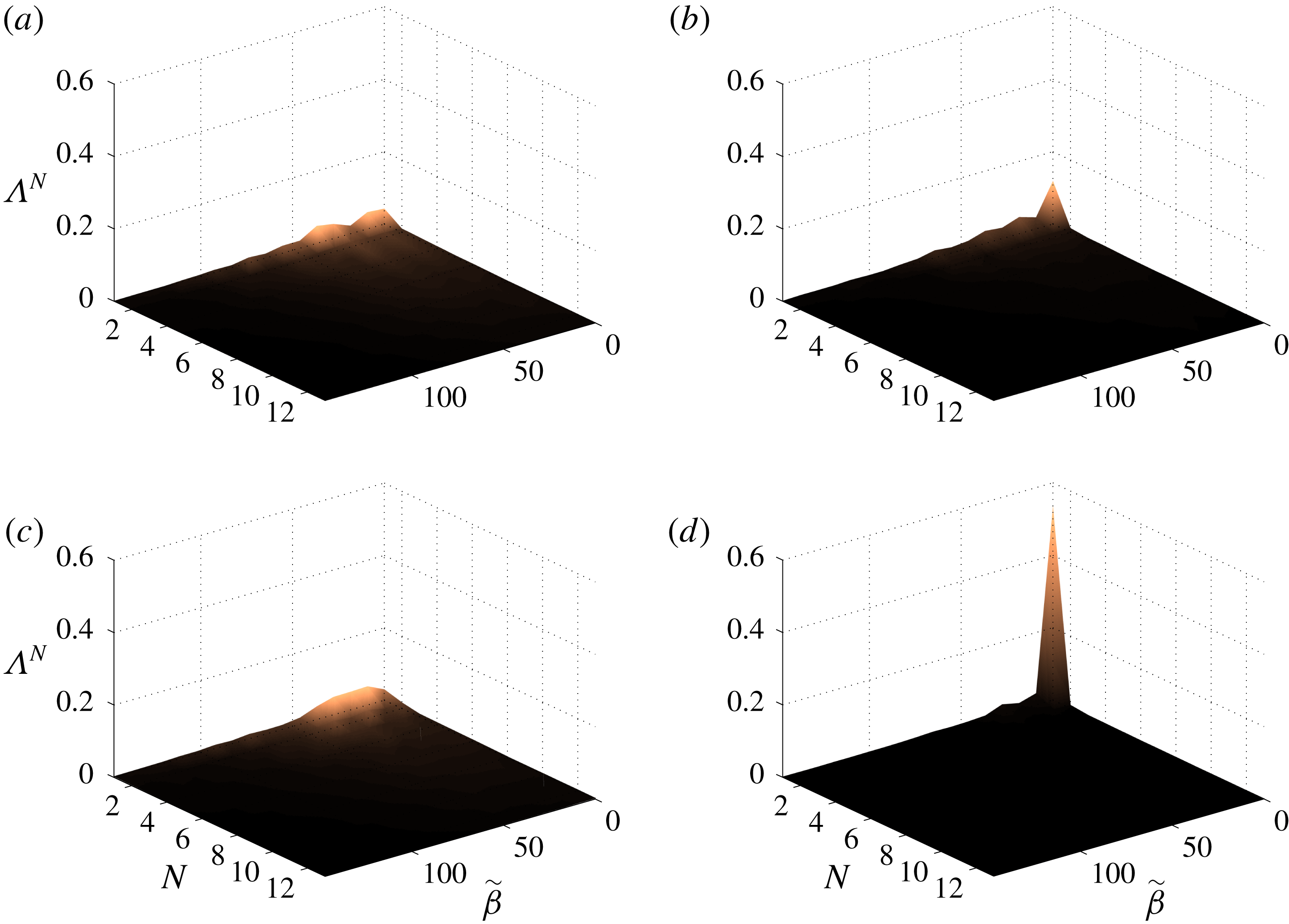
Normalized POD values corresponding to TKE metric for case $olA\unicode[STIX]{x1D6FC}4$ are shown in figure 11 as a function of non-dimensional spanwise wavenumber ( $\tilde{\unicode[STIX]{x1D6FD}}=2\unicode[STIX]{x03C0}c_{slat}/\unicode[STIX]{x1D706}_{z}$ , where $\unicode[STIX]{x1D706}_{z}$ is the spanwise wavelength) and mode number ( $N$ ). Results for four frequencies are presented, three corresponding to narrowband peaks in the noise spectrum ( $St=1.88$ , 2.76 and 3.53) and one corresponding to broadband noise ( $St=2.98$ ). The POD values for the first narrowband peak, figure 11(a), and for the broadband noise frequency, figure 11(c), are significantly spread over the spanwise wavenumber axis, revealing a highly three-dimensional character of the flow structures. On the other hand, the first mode with $\tilde{\unicode[STIX]{x1D6FD}}=0$ dominates the spectra for the second and third peaks, figures 11(b) and 11(d) respectively, indicating that the first two-dimensional (2-D) POD modes capture a substantial portion (approximately 10 % and 54 % respectively) of the turbulent kinetic energy associated with these narrowband peak frequencies.

Figure 12 shows the real part of the velocity components of the leading 2-D TKE-based POD mode at $St=3.53$ , a frequency of a narrowband peak. It is seen that the leading two-dimensional modes are localized along the mixing-layer path. The shape of this mode’s $x$ - and $y$ -velocity components strongly relates it to the K–H instability. An analogous picture is obtained for the first 2-D POD mode for all other frequencies. Figure 13 shows the real part of the velocity components of dominant POD mode for the broadband noise frequency of figure 11(c). The mode seems to represent spanwise modulated K–H vortices and 3-D fluctuations in the slat wake. The real part of the velocity components of the first $(St,\tilde{\unicode[STIX]{x1D6FD}})=(1.88,36.6)$ TKE-based POD mode corresponding to a peak frequency is shown in figure 14. It captures an amount of energy comparable to the first 2-D mode for the same frequency and reveals structures in the slat that represent predominantly streamwise stretched vortices being ejected through the gap (Imamura et al. Reference Imamura, Enomoto, Yokokawa and Yamamoto2008; Deck & Laraufie Reference Deck and Laraufie2013).

Figure 12.

Real part of the velocity components of the turbulent-kinetic-energy-based POD mode for $(St,\tilde{\unicode[STIX]{x1D6FD}})=(3.53,0)$ (narrowband peak) from case $olA\unicode[STIX]{x1D6FC}4$ . (a) Streamwise, (b) vertical and (c) spanwise components.

Figure 13.

Real part of the velocity components of the turbulent-kinetic-energy-based POD mode for $(St,\tilde{\unicode[STIX]{x1D6FD}})=(2.98,9.2)$ (broadband noise) from case $olA\unicode[STIX]{x1D6FC}4$ . (a) Streamwise, (b) vertical and (c) spanwise components.

Figure 14.

Real part of the velocity components of the turbulent-kinetic-energy-based POD mode for $(St,\tilde{\unicode[STIX]{x1D6FD}})=(1.88,36.6)$ (narrowband peak) from case $olA\unicode[STIX]{x1D6FC}4$ . (a) Streamwise, (b) vertical and (c) spanwise components.

POD values based on the acoustic pressure metric applied to the case $olA\unicode[STIX]{x1D6FC}4$ are given in figure 15, showing the dominance of the first two-dimensional mode, both for frequencies associated with narrowband peaks and for frequencies of broadband noise. The acoustic ‘energy’ captured by the leading 2-D POD is at least 70 % of the total in all cases analysed, being higher than 90 % for some narrowband peak frequencies, which indicates that the far-field pressure fluctuations below the airfoil are strongly coherent over the span. The real part of the velocity components of the leading POD mode based on the acoustic pressure for $St=3.53$ (a narrowband peak frequency) are shown in figure 16. Similar to the dominant TKE-based POD mode, for this frequency, the dominant acoustic-based POD mode resembles the K–H vortices. Kelvin–Helmholtz vortices were found to dominate the first 2-D acoustic-pressure-based POD modes for the other frequencies as well.

Figure 15.

Acoustic-based normalized POD values from case $olA\unicode[STIX]{x1D6FC}4$ at selected frequencies: (a) $St=1.88$ (narrowband peak), (b) $St=2.76$ (narrowband peak), (c) $St=2.98$ (broadband) and (d) $St=3.53$ (narrowband peak).

Figure 16.

Real part of the velocity components of the acoustic-based POD mode for $(St,\tilde{\unicode[STIX]{x1D6FD}})=(3.53,0)$ (narrowband peak) from case $olA\unicode[STIX]{x1D6FC}4$ . (a) Streamwise, (b) vertical and (c) spanwise components.

The POD analysis was extended to the other configurations. For the cases $olA\unicode[STIX]{x1D6FC}8$ and $olB\unicode[STIX]{x1D6FC}4$ , the TKE-based POD spectra are dominated by the first 2-D mode at the frequencies of the narrowband peaks, while the corresponding spectra were dominated by three-dimensional POD modes at broadband noise frequencies. Although case $olC\unicode[STIX]{x1D6FC}4$ does not present the peaks, its TKE-based POD spectrum has a 2-D dominant mode for some of the frequencies analysed. Moreover, the 2-D TKE-based POD modes for these three other cases are dominated by structures resembling the K–H waves in the mixing layer, as shown in figure 17, while 3-D TKE-based POD modes represent energetic structures in the mixing layer, and also in the slat gap and wake (figure 18). Also in line with the observations for case $olA\unicode[STIX]{x1D6FC}4$ , spanwise-coherent pressure fluctuations dominate in the far field for the other conditions tested. For these other three cases, the first 2-D acoustic-pressure-based POD mode captures more than 60 % of the energy of the far-field pressure fluctuations, and resembles K–H structures in the mixing layer regardless of the frequency corresponding to narrowband peak or broadband noise.

Figure 17.

Real part of the velocity components of the turbulent-kinetic-energy-based POD mode for $(St,\tilde{\unicode[STIX]{x1D6FD}})=(5.63,0)$ from case $olC\unicode[STIX]{x1D6FC}4$ . (a) Streamwise, (b) vertical and (c) spanwise components.

Figure 18.

Real part of the velocity components of the turbulent-kinetic-energy-based POD mode for $(St,\tilde{\unicode[STIX]{x1D6FD}})=(5.63,36.8)$ from case $olC\unicode[STIX]{x1D6FC}4$ . (a) Streamwise, (b) vertical and (c) spanwise components.

In summary, the POD analysis showed that for all frequencies analysed the slat noise is correlated to spanwise aligned structures even if they are not the most energetic ones. Although our analysis so far does not reveal the frequency selection mechanism, it is consistent with a feedback loop: the sound emitted at the slat’s trailing edge being fundamentally two-dimensional triggers spanwise-coherent K–H structures at the cusp. At narrowband peaks the sound is loud and leads to a prevalence of spanwise-coherent structures in the flow field. Off the peaks they become considerably more three-dimensional.

4.1 Evidences of the feedback mechanism

Terracol et al. (Reference Terracol, Manoha and Lemoine2016) proposes a feedback loop model for the generation of the narrowband peaks in the slat noise spectrum, which is inspired in the classical Rossiter (Reference Rossiter1966) model for the generation of acoustic tones by an open cavity flow: a pressure wave introduces a disturbance in the mixing layer at the slat cusp; this disturbance is amplified due to the mixing-layer instability as it is advected towards the reattachment point; then the large amplitude disturbance impinges on the slat cove surface generating a new pressure wave front; finally, this new pressure disturbance travels upstream exciting the mixing-layer instability at the cusp. Denoting the distance travelled by the mixing-layer disturbance from the cusp to the reattachment point by $L_{v}$ , the distance travelled by the pressure wave (assuming a straight path from the reattachment to the cusp) by $L_{a}$ , the mixing-layer disturbance phase velocity by $U_{v}$ , and neglecting convective effects on the acoustic propagation since the Mach number is too low, this model results in a series of discrete frequencies

(4.1) $$\begin{eqnarray}St_{n,Terracol}=n\frac{c_{slat}}{U_{\infty }}\left(\frac{L_{v}}{U_{v}}+\frac{L_{a}}{c_{\infty }}\right)^{-1},\end{eqnarray}$$

where $n=1,2,3,\ldots ,$ and $c_{\infty }$ is the free-stream sound speed.

The values of $L_{v}$ , $L_{a}$ and $U_{v}$ are estimated from the simulations based on the time-averaged mixing-layer path (figure 19 a) and time-averaged velocity along it $\overline{U}$ (figure 19 b), where $\tilde{S}=S/L_{v}$ and $S$ is the distance to the cusp along the mixing-layer path. As opposed to Terracol et al. (Reference Terracol, Manoha and Lemoine2016), not all our cases presented a plateau in the $\overline{U}$ distribution. To circumvent this difficulty $U_{v}$ is estimated as the averaged velocity between $\tilde{S}\approx 0.15$ and $\tilde{S}\approx 0.85$ , which is an interval of mild acceleration in cases $olA\unicode[STIX]{x1D6FC}4$ and $olA\unicode[STIX]{x1D6FC}8$ and of the plateau in cases $olB\unicode[STIX]{x1D6FC}4$ and $olC\unicode[STIX]{x1D6FC}4$ . The normalized values of $L_{v}$ , $L_{a}$ and $U_{v}$ are listed in table 3 and the peak frequencies predicted from (4.1) are listed in table 4 and compared to the peak frequencies of the spectra computed from the simulation data (figure 9). For the cases where the peaks are observed, the predicted frequencies are in fair agreement with the peak frequencies computed from the FW–H data, comparable to that achieved by Deck & Laraufie (Reference Deck and Laraufie2013) using a similar methodology.

Figure 19.

(a) Time-averaged mixing-layer path with indication of four stages of the mixing-layer disturbance evolution and (b) time-averaged velocity along the mixing layer (horizontal lines represent the mean velocity between $\tilde{S}\approx 0.15$ and 0.85). Black: case $olA\unicode[STIX]{x1D6FC}4$ , red: $olA\unicode[STIX]{x1D6FC}8$ , blue: $olB\unicode[STIX]{x1D6FC}4$ and green: $olC\unicode[STIX]{x1D6FC}4$ .

Table 3.

Normalized time-averaged flow properties of the slat mixing layer. $U_{v}$ is the estimated phase velocity of the mixing-layer disturbance.

It must be said, however, that since the velocity changes abruptly outside the interval between 15 and 85 %, the estimation of $U_{v}$ is highly sensitive to broader limits. Moreover, although Terracol’s model is able to provide fairly accurate predictions of the narrowband peaks observed in their slat noise spectrum as well as for the four cases simulated here, it is difficult to reconcile this model with the evidence that the slat trailing edge is the acoustic emission spot, as suggested by the approximate $U_{\infty }^{5}$ velocity scaling law (Dobrzynski et al. Reference Dobrzynski, Nagakura, Gehlhar and Bushbaum1998) and the spatial directivity pattern (Lockard & Choudhari Reference Lockard and Choudhari2009; Ewert et al. Reference Ewert, Dierke, Pott-Pollenske, Appel, Emunds and Sutcliffe2010). Furthermore, as indicated in figure 17, the dynamics of the 2-D mixing-layer structures for the case $olC\unicode[STIX]{x1D6FC}4$ is similar to the other cases both qualitatively and quantitatively. Therefore, there is no apparent reason for the complete attenuation of the narrowband peaks for that case according to this model.

Table 4.

Discrete peak Strouhal numbers. Comparison between values computed by the FW–H algorithm applied to the LBM computations (denoted by $\text{LBM}+\text{FW}{-}\text{H}$ ), values predicted by the formula $St_{n,Terracol}$ (4.1) and the values predicted by (4.5).

Figure 20 shows contour plots of the magnitude of the pressure component of the dominant acoustic-based POD mode, indicating the trajectory of the K–H vortices within the cove. The white line marks the maximum amplitude of the POD structures and gives an indication of the vortex path. The red dashed line is the dividing streamline linking the cusp to the reattachment point (shown in figure 19 a). It is observed that, for all cases, the vortices travel along the dividing streamline for a long length, but divert from it close the reattachment point. This suggests a different path for the feedback loop concept, which is described schematically in figure 21: (i) at a reference time $t=0$ , the mixing layer is disturbed at the slat cusp; (ii) the disturbance amplifies as it travels along the mixing-layer path; (iii) at $t=T_{h}$ , a sound wave front is emitted as the disturbance interacts with the slat trailing edge after travelling the mixing-layer length $L_{v}^{\prime }$ plus a distance $\unicode[STIX]{x1D6EC}$ , which accounts for a possible delay between the passage of the mixing-layer disturbance at the trajectory point closest to the trailing edge and the acoustic wave emission (Such phase difference is also accounted for by Rossiter (Reference Rossiter1966) for open cavities); (iv) the sound wave travels downstream at approximately the free-stream sound speed $c_{\infty }$ and reaches the slat cusp introducing a new disturbance in the mixing layer at $t=T_{h}+L_{a}^{\prime }/c_{\infty }$ , where $L_{a}^{\prime }$ is the distance between the slat trailing edge and the cusp. The coordinate $S^{\prime }$ starts from the cusp along the mixing-layer path, goes through the trailing edge and back to the cusp along a straight line (acoustic path). This loop concept circumvents the difficulties raised in last paragraph and results in discrete peak frequencies given by

(4.2) $$\begin{eqnarray}St_{n}=n\frac{c_{slat}}{U_{\infty }}\left(T_{h}+\frac{L_{a}^{\prime }}{c_{\infty }}\right)^{-1}.\end{eqnarray}$$

It is admitted that, in view of long acoustic wavelength, it can be difficult to distinguish a source at the trailing edge from one at the reattachment point. However, the results discussed hereinafter provide evidence of this distinction.

Figure 20.

Path of the mixing-layer disturbances (solid line) estimated from the amplitude of the pressure component of the dominant acoustic-based POD mode (colour plot) for cases (a) $olA\unicode[STIX]{x1D6FC}4$ , (b) $olA\unicode[STIX]{x1D6FC}8$ , (c) $olB\unicode[STIX]{x1D6FC}4$ and (d) $olC\unicode[STIX]{x1D6FC}4$ . The time-averaged streamline from figure 19(a) is shown for comparison (dashed lines).

Figure 21.

Schematic representation of the Rossiter-like feedback loop.

Figure 22.

Real part of the evolution of the dominant acoustic-based POD mode for $St=3.53$ ( $\tilde{\unicode[STIX]{x1D719}}(x,y,\tilde{t},St=3.53;\tilde{\unicode[STIX]{x1D6FD}}=0)$ ) from case $olA\unicode[STIX]{x1D6FC}4$ at selected times, where $\tilde{t}=tU_{\infty }St/c_{slat}$ is the non-dimensional time. (a) $\tilde{t}=0$ , (b) $\tilde{t}=5/18$ and (c)  $\tilde{t}=3/4$ .

In order to search for confirmation of this feedback loop, the temporal evolution of the dominant acoustic-based POD modes,

(4.3) $$\begin{eqnarray}\tilde{\unicode[STIX]{x1D753}}(x,y,\tilde{t};St)=\text{Re}\{\hat{\unicode[STIX]{x1D753}}_{1}(x,y;St,\tilde{\unicode[STIX]{x1D6FD}}=0)\text{e}^{\text{i}2\unicode[STIX]{x03C0}\tilde{t}}\},\end{eqnarray}$$

is analysed, where $\hat{\unicode[STIX]{x1D753}}_{1}(x,y;St;\tilde{\unicode[STIX]{x1D6FD}}=0)$ is the first two-dimensional acoustic-based POD mode at $St$ and $\tilde{t}=tU_{\infty }St/c_{slat}$ is the non-dimensional time.

Figure 22 shows the pressure component of $\tilde{\unicode[STIX]{x1D753}}(x,y,\tilde{t};3.53)$ for selected times based on case $olA\unicode[STIX]{x1D6FC}4$ . The left-hand side of the figure shows the extended region of the POD mode, where sound waves emanating from the slat cove can be identified, and the right-hand side shows a detailed view of the slat cove. The zoomed-in figure shows, for $\tilde{t}=0$ , a negative pressure mixing-layer disturbance reaching the reattachment point region, while in the open view, a compression wave is seen leaving the slat cove downwards. The interaction of the negative pressure mixing-layer disturbance and the slat surface generates an expansion wave which dominates the slat cove region at $\tilde{t}=5/18$ , as seen in the open view. Simultaneously, the pressure at the slat cusp reaches its most negative value along the loop. At $\tilde{t}=3/4$ , a negative pressure disturbance originates close to the cusp and the expansion wave has left the cove region travelling downwards. The series of events shown in figure 22 is consistent with the acoustic wave fronts leaving the slat cove downwards being generated by the interaction of the mixing-layer disturbances with the slat trailing edge. It also reveals a directivity and phase pattern that resembles a dipole at the slat trailing edge.

Figure 23 shows, as function of $\tilde{t}$ and $\tilde{S}^{\prime }=S^{\prime }/L_{v}^{\prime }$ (see figure 21) during six periods, the spatio-temporal evolution of the pressure fluctuation corresponding to the leading acoustic pressure POD mode for selected narrowband peak frequencies, for cases $olA\unicode[STIX]{x1D6FC}4$ , $olA\unicode[STIX]{x1D6FC}8$ and $olB\unicode[STIX]{x1D6FC}4$ ( $St=3.53$ , 3.31 and 3.09, respectively) and for the frequency $St=5.63$ for the case $olC\unicode[STIX]{x1D6FC}4$ . The left portion of the diagrams ( $\tilde{S}^{\prime }<1$ ) shows the journey of the K–H structures from the cusp to the slat trailing edge. The solid white lines represent the phase evolution of the vortices. The disturbance speed is approximately constant over most of the trajectory, but at the beginning the amplitudes are very small and the advection speed cannot be accurately defined. The right portion represents the acoustic wave journey, i.e. the straight line connecting the ends of the hydrodynamic paths in figure 21. For $\tilde{S}>1$ the phase speed is equal to $c_{\infty }$ . From $\tilde{S}=1$ to $\tilde{S}\approx 1.2$ the mode is dominated by the high amplitude K–H structures being advected towards the gap and, therefore, do not correspond to the acoustic pressure wave. For the largest portion of the trajectory, the free-stream sound speed is a good representation of the pressure disturbance speed. For all cases, the pressure wave has a $\unicode[STIX]{x03C0}/2$ phase shift relative to the mixing-layer disturbance at the emission spot.

The diagrams strongly indicate that the disturbances in the mixing layer are introduced by pressure waves which in turn are generated by the interaction of the mixing-layer structures with the slat surface, characterizing a feedback loop. Additionally, the diagrams show that the narrowband peaks at $St=3.53$ , 3.31 and 3.09 for cases $olA\unicode[STIX]{x1D6FC}4$ , $olA\unicode[STIX]{x1D6FC}8$ and $olB\unicode[STIX]{x1D6FC}4$ respectively correspond to the fourth Rossiter-like mode: closure of the feedback loop by a particular K–H structure, as illustrated by the solid white lines in figure 23, requires four fundamental periods of its corresponding frequency. This is consistent with the observations on the noise spectra because, as can be inferred from table 4, the frequency shift between the narrowband peaks is approximately a quarter of the frequency of the modes shown in figure 23. It is possible to observe a consistent cycle even in case $olC\unicode[STIX]{x1D6FC}4$ , although the acoustic wave evolution looks severely distorted and ill defined.

The dashed white lines in figure 23 represent the averaged phase velocity of the mixing-layer structures in their trajectory from the cusp to the trailing edge. These velocities are slightly higher than the ones in table 3, except for the case $olC\unicode[STIX]{x1D6FC}4$ , for which the velocity is significantly higher. Adopting a simplification of uniform mixing-layer disturbance phase velocity equal to the ones represented by the dashed lines, and given the observed phase shift of $\unicode[STIX]{x03C0}/2$ , one can write

(4.4) $$\begin{eqnarray}T_{h}=\frac{L_{v}^{\prime }}{V}+\frac{\unicode[STIX]{x1D6EC}}{V}=\frac{L_{v}^{\prime }}{V}-\frac{c_{slat}}{4U_{\infty }St_{n}}.\end{eqnarray}$$

Substituting in (4.2),

(4.5) $$\begin{eqnarray}St_{n}=\frac{4n+1}{4}\times \frac{c_{slat}}{U_{\infty }}\times \frac{V}{L_{v}^{\prime }+\frac{V}{c_{\infty }}L_{a}^{\prime }}.\end{eqnarray}$$

Table 4 also presents the narrowband peak frequency predicted by this equation and shows, in general, an improvement comparing to the predictions based on Terracol’s formula.

Figure 23.

Spatio-temporal evolution of the pressure component of dominant acoustic POD mode for narrowband peak frequencies: (a) $St=3.53$ for the case $olA\unicode[STIX]{x1D6FC}4$ , (b) $St=3.31$ for the case $olA\unicode[STIX]{x1D6FC}8$ (c) $St=3.09$ for the case $olB\unicode[STIX]{x1D6FC}4$ and (d)  $St=5.63$ for the case $olC\unicode[STIX]{x1D6FC}4$ along $\tilde{S^{\prime }}=S^{\prime }/L_{v}^{\prime }$ (see figure 21). White solid lines represent phase evolutions where the phase speed is equal to $c_{\infty }$ for $\tilde{S^{\prime }}>1$ and follow maxima of the POD mode along the mixing-layer path.

4.2 Strength of the feedback mechanism

These results evidence the frequency selection mechanism unequivocally. However, they do not indicate what conditions enhance or prevent sound emission. In Rossiter’s cavity model, the magnitude of a mode is primarily a result of the amplification of the disturbances along the mixing layer (Rowley, Colonius & Basu Reference Rowley, Colonius and Basu2002; Sun et al. Reference Sun, Taira, Cattafesta III and Ukeiley2017). Figure 24 shows spectra of the streamwise velocity fluctuations at four points representing four stages of evolution of the mixing-layer disturbances discussed by Pagani et al. (Reference Pagani, Souza and Medeiros2016). Each spectrum is the average of the windowed blocks and the 32 points equally spaced in the spanwise direction. The location of the representative points is indicated in figure 19(a). The initial amplitude is larger for the noisiest case, which is consistent with a feedback loop. However, the largest amplitude growth is found to correlate with the lowest acoustic emission, as opposed to Rossiter cavity modes.

Figure 24.

PSD of streamwise velocity component in four mixing-layer evolution stages, stage 1 (cyan), stage 2 (grey), stage 3 (magenta), stage 4 (black). Cases (a) $olA\unicode[STIX]{x1D6FC}4$ , (b) $olA\unicode[STIX]{x1D6FC}8$ , (c) $olB\unicode[STIX]{x1D6FC}4$ and (d) $olC\unicode[STIX]{x1D6FC}4$ .

Figure 17 shows a tendency for the leading 2-D TKE-based POD mode to attenuate from the reattachment point to the trailing edge. This is important, because the acoustic-based POD analysis demonstrated that only 2-D structures are associated with sound. Iso-surfaces of the $\unicode[STIX]{x1D706}_{2}$ criterion in figure 25 clearly show streamwise oriented vortices in the gap region, similar to the ones identified by Imamura et al. (Reference Imamura, Enomoto, Yokokawa and Yamamoto2008) and Deck & Laraufie (Reference Deck and Laraufie2013). These vortices are likely to be due to the accelerating flow field in the vicinity of the main element leading edge (see figure 26), as first explained by Batchelor & Proudman (Reference Batchelor and Proudman1954).

Figure 25.

Iso-surfaces of $\unicode[STIX]{x1D706}_{2}$ in the slat cove. (a) $\unicode[STIX]{x1D706}_{2}=-20\,000$ for $olA\unicode[STIX]{x1D6FC}4$ ; (b) $\unicode[STIX]{x1D706}_{2}=-20\,000$ for $olA\unicode[STIX]{x1D6FC}8$ ; (c) $\unicode[STIX]{x1D706}_{2}=-5000$ for $olB\unicode[STIX]{x1D6FC}4$ ; (d) $\unicode[STIX]{x1D706}_{2}=-20000$ for $olC\unicode[STIX]{x1D6FC}4$ .

Figure 26.

Averaged Mach number field in the slat cove region. Cases (a) $olA\unicode[STIX]{x1D6FC}4$ ; (b) $olA\unicode[STIX]{x1D6FC}8$ ; (c) $olB\unicode[STIX]{x1D6FC}4$ ; (d) $olC\unicode[STIX]{x1D6FC}4$ .

Figure 27.

Averaged velocity (solid lines) and amplitude of planar velocity components of the turbulent-kinetic-energy-based dominant POD modes. Black: $St=3.53$ for case $olA\unicode[STIX]{x1D6FC}4$ , red: $St=3.31$ for case $olA\unicode[STIX]{x1D6FC}8$ , blue: $St=3.09$ for case $olB\unicode[STIX]{x1D6FC}4$ and green: $St=5.67$ for case $olC\unicode[STIX]{x1D6FC}4$ .

Figure 27 shows the evolution of the planar velocity magnitude ( $|\unicode[STIX]{x1D719}_{uv}|=(|\unicode[STIX]{x1D719}_{u}|^{2}+|\unicode[STIX]{x1D719}_{v}|^{2})^{0.5}$ , where $\unicode[STIX]{x1D719}_{u}$ and $\unicode[STIX]{x1D719}_{v}$ are the $x$ and $y$ velocity components) of the leading 2-D TKE-based POD mode for representative frequencies. The time-spanwise-averaged flow speed along the disturbance path is also shown in the figure revealing that the energy decay of the 2-D disturbances correlates well with the flow acceleration downstream of the reattachment point. In turn, the magnitude of flow acceleration correlates well with the noise suppression. This observation is consistent with the argument that the accelerating flow field favours three-dimensionalization of the mixing-layer structures, reducing the sound emission. This may explain the variation of sound emission observed for the different configurations and, in particular, the absence of the narrowband peaks in the $olC\unicode[STIX]{x1D6FC}4$ case noise spectrum.