1 Introduction
Mixing in fluids is a basic process controlling transport and chemical reactions in many natural and industrial systems (e.g. Ottino Reference Ottino1989; Tel et al. Reference Tel, de Mourab, Grebogib and Károlyid2005; Dentz et al. Reference Dentz, LeBorgne, Englert and Bijeljic2011); it remains, in random flows, a fascinating scientific challenge (Batchelor Reference Batchelor1959; Kraichnan Reference Kraichnan1994; Shraiman & Siggia Reference Shraiman and Siggia2000; Falkovich, Gawedzki & Vergassola Reference Falkovich, Gawedzki and Vergassola2001; Tartakovsky, Tartakovsky & Meakin Reference Tartakovsky, Tartakovsky and Meakin2008; Jha, Cueto-Felgueroso & Juanes Reference Jha, Cueto-Felgueroso and Juanes2011; Ye et al. Reference Ye, Chiogna, Cirpka, Grathwohl and Roll2015). The analysis and modelling of the temporal dynamics of concentration distributions has been the subject of numerous studies for a variety of flows. In all of them, the repeated action of advective fluid motion is known to create complex spatial structures, characterized by elongated lamellar (in two dimensions), or sheets (in three dimensions) patterns which promote mixing by augmenting the area available for diffusive transfer, and reducing mixing times (Ranz Reference Ranz1979; Ottino Reference Ottino1989; Villermaux Reference Villermaux2012b ; de Anna et al. Reference de Anna, Dentz, Tartakovsky and Le Borgne2014a ).
The concentration content of mixtures as they evolve towards uniformity is quantified from the temporal evolution of the concentration probability density function (PDF). The latter is described precisely within a general frame decomposing a complex mixture into a set of elementary lamellae (sheets) whose concentration decay under the action of the flow stretching, and possibly merge with their neighbours in the contracting regions of the flow, when they are not too dispersed from each other (Villermaux & Duplat Reference Villermaux and Duplat2003). Decay and aggregation compensate when the average concentration is conserved, as in confined mixtures (Duplat & Villermaux Reference Duplat and Villermaux2008), while a lack of aggregation for a given flow stirring strength leads to dilution of dispersing mixtures (Duplat, Innocenti & Villermaux Reference Duplat, Innocenti and Villermaux2010). Precise predictions of the PDF shapes and rate of deformation are obtained in flows where the encounter between interacting lamellae is made at random. The corresponding flows, which empirically happen to be the rule rather than exceptions, may not be strongly turbulent, but only require to be random, as just defined. Indeed, the corresponding approach has also been successful for very different classes of flows, including turbulent flows (Duplat & Villermaux Reference Duplat and Villermaux2008; Duplat et al. Reference Duplat, Innocenti and Villermaux2010), chaotic flows (Meunier & Villermaux Reference Meunier and Villermaux2010), microfluidic flows (Villermaux, Stroock & Stone Reference Villermaux, Stroock and Stone2008), and porous media flows (Le Borgne, Dentz & Villermaux Reference Le Borgne, Dentz and Villermaux2013). In this framework, the statistical properties and the degree of smoothness of the underlying velocity fields is embedded into two main elements that are sufficient for predicting concentration distributions: the distribution of stretching rates, which governs the concentration decay of elementary lamella, and the spatial distribution of lamella density, which controls their probability of encounter.
Many processes, however, depend on concentration gradients, or differences
 $\unicode[STIX]{x0394}c$
taken at a given spatial increment
 $\unicode[STIX]{x0394}x$
, rather than on the concentration amplitudes
 $c$
themselves. This includes a wide range of chemical reactions, such as redox reactions, mixing-driven precipitation, and rock dissolution (Dentz et al.
Reference Dentz, LeBorgne, Englert and Bijeljic2011; de Anna et al.
Reference de Anna, Jimenez-Martinez, Tabuteau, Turuban, Le Borgne, Derrien and Meheust2014b
; Bolster Reference Bolster2014; Haudin et al.
Reference Haudin, Cartwright, Brau and De Wit2014; Le Borgne, Ginn & Dentz Reference Le Borgne, Ginn and Dentz2014; Fu et al.
Reference Fu, Cueto-Felgueroso, Bolster and Juanes2015; Paster, Aquino & Bolster Reference Paster, Aquino and Bolster2015), and biological processes in fluids, such as chemotaxis (Tel et al.
Reference Tel, de Mourab, Grebogib and Károlyid2005; Vergassola, Villermaux & Shraiman Reference Vergassola, Villermaux and Shraiman2007; Neufeld & Hernandez-Garcia Reference Neufeld and Hernandez-Garcia2009; Stocker Reference Stocker2012; Taylor & Stocker Reference Taylor and Stocker2012). It is also, since Kolmogorov, customary in the turbulence community to study spatial differences of the field (velocity, temperature, concentration) rather than the field itself (Monin & Yaglom Reference Monin and Yaglom1975). A large body of experiments, notably in the context of turbulence (Antonia et al.
Reference Antonia, Hopfinger, Gagne and Anselmet1984; Vaienti et al.
Reference Vaienti, Ould-Rouis, Anselmet and Le Gal1995; Warhaft Reference Warhaft2000), has shown that the distribution of the concentration increments depends in a non-trivial way on the separation distance: its shape does not deform self-similarly as
 $\unicode[STIX]{x0394}x$
varies, it presents a peak in
 $\unicode[STIX]{x0394}c=0$
and heavy large excursion tails (for, say,
 $|\unicode[STIX]{x0394}c|$
much larger than its typical root mean squared value), that are all the more pronounced as
 $\unicode[STIX]{x0394}x\rightarrow 0$
.
This puzzling so-called intermittent behaviour has received great attention over the years (see e.g. Frisch Reference Frisch1995) and, in the passive scalar context (see Falkovich et al. Reference Falkovich, Gawedzki and Vergassola2001), has prompted a wealth of original ideas (Oboukhov Reference Oboukhov1962; Kraichnan Reference Kraichnan1974; Pumir, Shraiman & Siggia Reference Pumir, Shraiman and Siggia1991; Kraichnan Reference Kraichnan1994; Vaienti et al. Reference Vaienti, Ould-Rouis, Anselmet and Le Gal1994; Balkovsky & Fouxon Reference Balkovsky and Fouxon1999; Kalda & Morozenko Reference Kalda and Morozenko2008), all of them emphasizing the necessary coupling between the structure of the stirring field (i.e. the velocity differences) and the resulting properties of the scalar field (its gradients in particular), with almost no exception (see however Kalda Reference Kalda2000).
We develop here a substantially different point of view. Our theory does not assume any anomaly, nor any particular scaling structure of the stirring field. On the contrary, our approach only requires randomness, that of the stirring fields in which the construction of the scalar field is a process of random aggregation of stretched lamellae (Villermaux & Duplat Reference Villermaux and Duplat2003). We thus envisage the question of the concentration increments as a deconstruction process: since every concentration level is the sum of a number of contributions from elementary lamellae (see figure 1 c), taking differences between two distant points amounts to cancelling out those contributions which are common to the two assemblages, if any. It will be seen that the spatial correlation in the scalar field can be inferred by quantifying the common aggregation history of points separated by a given distance in the field. A first application of this principle for quantifying concentration increments in porous media flows was presented by Le Borgne, Dentz & Villermaux (Reference Le Borgne, Dentz and Villermaux2015), for the limiting cases of very low and very large Peclet numbers. Here we generalize the increment PDF theory to (i) demonstrate its relevance for turbulent flows, (ii) cover the full range of Peclet numbers for porous media, and (iii) show the emergence of intermittency under incomplete aggregation processes. Hence, we derive explicit expressions for the PDF of concentration increments for a variety of mixtures (turbulent plume, channel flow, porous medium) and lamellae interaction regimes (complete, partial or no aggregation).
In § 2 we first present the general theory for concentration increments under lamella stretching and aggregation. We then apply these concepts to three different flows, representative of the range of spatial patterns that control scalar gradients in fluids. For all these cases, we recall previous results obtained for the concentration PDFs, which are needed for deriving the concentration increment PDFs. In § 3 we apply the theory to mixing of a plume in a turbulent jet, with minimal aggregation. In § 4 we consider the case of fully developed aggregation in a confined turbulent mixture. In § 5 we discuss the development of a partial aggregation regime, characterized by strong intermittency, for the case of mixing in porous media. In § 6 we derive analytical expressions for structure functions and discuss the conditions for intermittency. Section 7 considers in particular the case of heterogeneous mixtures.
2 Increments under lamella stretching and aggregation
We review here the basic concepts for characterizing concentration increments, and we present a general theoretical framework for predicting their PDFs based on the composition rules of scalar fields from stretched lamellae aggregation (figure 1). The key question that we address is how to relate the concentration increment PDFs to the concentration PDFs. While the latter have been well studied in the framework of lamellar mixing theories (Villermaux & Duplat Reference Villermaux and Duplat2003; Duplat & Villermaux Reference Duplat and Villermaux2008; Duplat et al. Reference Duplat, Innocenti and Villermaux2010; Le Borgne et al. Reference Le Borgne, Dentz and Villermaux2013), concentration increment PDFs have been described in this framework so far in the context of porous media flows, considering idealized cases of very low or very high Peclet numbers (Le Borgne et al. Reference Le Borgne, Dentz and Villermaux2015), and mixtures composed of independent lamellae (Meunier & Villermaux Reference Meunier and Villermaux2010). Here we generalize the random aggregation theory for concentration increments, showing its relevance for different types of flows and Peclet numbers, and thus providing a link between incomplete aggregation and intermittency.
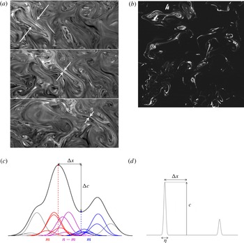
(a) Three consecutive instants of time showing how a bundle of stretched sheets in a confined channel are brought together and merge, losing their individuality on a support of transverse thickness
 $\unicode[STIX]{x1D702}$
. (b) Close-up in the dispersing mixture showing how the scalar field resolves into a set of essentially non-interacting, disjointed sheets with distributed concentrations (see figure 2
a, for details). (c) Sketch of the elementary sheet overlapping mechanism constructing the concentration field. The concentration field (black line) is made by the random superposition of
 $n$
sheets (coloured lines). Hence, the concentration located at the red point receives contributions from the red curves and the purple curves, while the concentration located at the blue point receives contributions from the blue curves and the purple curves. When considering the difference in concentration between these two points, the contributions from the purple sheets statistically cancel out, and thus the concentration increment
 $\unicode[STIX]{x0394}c$
is determined by
 $m$
independent sheets (in red and blue), with
 $m\leqslant n$
. (d) In dispersing mixtures where sheets are isolated and merging is anecdotal, concentration differences
 $\unicode[STIX]{x0394}c$
are given by the concentration field
 $c$
itself.

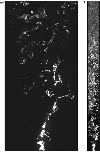
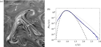
(a) A planar cut through a dispersing plume made by the injection of a dye (disodium fluorescein in water) through a small tube of
 $d=4~\text{mm}$
in diameter on the axis of a larger turbulent jet whose integral scale is
 $L=8~\text{cm}$
at the injection location. Scalar sheets dilute by evolving on their own. (b) Same as in (a), with the plume confined in a square duct of lateral width
 $L=3~\text{cm}$
. The mixture relaxes, through aggregation of sheets, towards a non-zero average concentration in that case. The Reynolds number of the flow is
 $Re=10^{4}$
.

2.1 Basic concepts
2.1.1 Concentration increment PDF
The spatial structure of scalar fields may be quantified from the PDF of concentration increments
 $p_{\unicode[STIX]{x0394}x}(\unicode[STIX]{x0394}c)$
, computed for spatial increments
 $\unicode[STIX]{x0394}x=|\unicode[STIX]{x0394}\boldsymbol{x}|$
, as
 $$\begin{eqnarray}\unicode[STIX]{x0394}c(\boldsymbol{x},t,\unicode[STIX]{x0394}x)=c(\boldsymbol{x}+\unicode[STIX]{x0394}\boldsymbol{x},t)-c(\boldsymbol{x},t).\end{eqnarray}$$
The proper gradient PDF is recovered when
 $\unicode[STIX]{x0394}x$
tends to zero. The dependence of the concentration increment PDFs on the spatial scale
 $\unicode[STIX]{x0394}x$
reflects the spatial structure of concentration fields arising from the combined action of molecular diffusion and stretching by the flow.
When a characteristic diffusive smoothing correlation scale
 $\unicode[STIX]{x1D702}$
can be defined for the scalar field (also called coarse graining scale, see e.g. Villermaux & Duplat Reference Villermaux and Duplat2006; Meunier & Villermaux Reference Meunier and Villermaux2010), the concentration increments over spatial increments
 $\unicode[STIX]{x0394}x$
larger than
 $\unicode[STIX]{x1D702}$
, denoted by
 $\unicode[STIX]{x0394}c^{{>}}$
, are the difference of independent (random) concentration values. In this case, the PDF
 $p_{\unicode[STIX]{x0394}x}(\unicode[STIX]{x0394}c)$
of concentration increments is obtained from the convolution of the global concentration PDF as
 $$\begin{eqnarray}p_{\unicode[STIX]{x0394}x>\unicode[STIX]{x1D702}}(\unicode[STIX]{x0394}c)=\int \,\text{d}c^{\prime }p_{c}(c^{\prime },t)p_{c}(c^{\prime }-\unicode[STIX]{x0394}c,t),\end{eqnarray}$$
where
 $p_{c}(c,t)$
is the concentration PDF – in general, a function of the residence time
 $t$
of the mixture in the stirred medium. This expression relates the concentration increment PDF to the concentration PDF, and it holds in absence of correlation. As discussed in the following, for increments
 $\unicode[STIX]{x0394}x$
smaller than the scalar field correlation length
 $\unicode[STIX]{x1D702}$
for which the concentration levels are correlated, additional information about the way the concentration field has been constructed is needed.
2.2 Ensemble of non-interacting lamellae
We first recall basic results for a mixture composed of isolated lamellae evolving solely under stretching and diffusion (figure 1 b,d). As discussed in the next section, this situation is relevant to dispersing mixtures in turbulent flows, where expansion of the scalar field support prevents elementary lamellae from overlapping and aggregating (Duplat et al. Reference Duplat, Innocenti and Villermaux2010), and in porous media flows at large Peclet numbers (Le Borgne et al. Reference Le Borgne, Dentz and Villermaux2015). At the lamella scale, the scalar concentration is close to uniform along the stretching direction, and varies rapidly in the compressive direction. The transverse concentration profile can be approximated by a Gaussian profile which is a solution to the one-dimensional compression diffusion equation (Meunier & Villermaux Reference Meunier and Villermaux2010). The corresponding concentration PDF is parametrized by the local maximum concentration, which depends on the lamella deformation history, driven by the Lagrangian velocity gradients experienced by the lamella. The overall PDF is a weighted average of this PDF over the lamellae stretching histories, reflecting the velocity gradient statistics.
For this type of scalar field, the correlation scale
 $\unicode[STIX]{x1D702}$
is equal to the characteristic lamella width, equilibrating the rates of substrate compression, and diffusing broadening. It is equal to the familiar Batchelor scale in exponentially stretched flows (Batchelor Reference Batchelor1959; Meunier & Villermaux Reference Meunier and Villermaux2010), or increases like
 $\sqrt{Dt}$
when the mean stretching decays in time (Duplat et al.
Reference Duplat, Innocenti and Villermaux2010; Villermaux Reference Villermaux2012b
; Le Borgne et al.
Reference Le Borgne, Dentz and Villermaux2013). For distances larger than the correlation scale
 $\unicode[STIX]{x1D702}$
, that is
 $\unicode[STIX]{x0394}x>\unicode[STIX]{x1D702}$
, the increment PDF is given by (2.2) since concentration levels are independent. For
 $\unicode[STIX]{x0394}x<\unicode[STIX]{x1D702}$
, Meunier & Villermaux (Reference Meunier and Villermaux2010) have shown that a linear interpolation of the local Gaussian concentration distributions provides a good approximation for the concentration increment distributions at the lamella scale. Under this approximation the concentration increment
 $\unicode[STIX]{x0394}c^{{<}}$
for
 $\unicode[STIX]{x0394}x<\unicode[STIX]{x1D702}$
is related to
 $\unicode[STIX]{x0394}c^{{>}}$
as
 $$\begin{eqnarray}\unicode[STIX]{x0394}c^{{<}}=\frac{\unicode[STIX]{x0394}x}{\unicode[STIX]{x1D702}}\unicode[STIX]{x0394}c^{{>}}.\end{eqnarray}$$
This simple linear approximation of the concentration profile across a lamella allows relating the PDF of concentration increments for lag distances
 $\unicode[STIX]{x0394}x<\unicode[STIX]{x1D702}$
to the PDF of concentration increments for lag distances greater than the correlation scale
 $\unicode[STIX]{x1D702}$
, which is independent of
 $\unicode[STIX]{x0394}x$
. Hence, the PDF of concentration increments
 $\unicode[STIX]{x0394}c^{{<}}$
can be written in terms of the PDF of
 $\unicode[STIX]{x0394}c^{{>}}$
as (Meunier & Villermaux Reference Meunier and Villermaux2010)
 $$\begin{eqnarray}p_{\unicode[STIX]{x0394}x<\unicode[STIX]{x1D702}}(\unicode[STIX]{x0394}c)=\frac{\unicode[STIX]{x1D702}}{\unicode[STIX]{x0394}x}p_{\unicode[STIX]{x0394}x>\unicode[STIX]{x1D702}}\left(\frac{\unicode[STIX]{x1D702}}{\unicode[STIX]{x0394}x}\unicode[STIX]{x0394}c\right).\end{eqnarray}$$
In the absence of overlap between lamellae, the derivation of concentration increments is thus relatively simple, since neighbouring concentration levels are either deterministically correlated (for
 $\unicode[STIX]{x0394}x<\unicode[STIX]{x1D702}$
) or uncorrelated (for
 $\unicode[STIX]{x0394}x>\unicode[STIX]{x1D702}$
). The concentration increment PDFs is thus directly related to the concentration PDF, as described above, and hence to the velocity gradient statistics. Interactions between lamellae induce less trivial spatial correlations in the scalar field, which are the main focus of this study.
2.3 Concentration increments under random aggregation processes
We now consider the regime where the lamellae are close to each other, and interact by merging through diffusive coalescence (figure 1
a). This encompasses a large class of scalar fields in different types of flows, in which spatial correlations exist over a range of scales. Diffusive overlap between elementary lamellae occurs in bundles (Villermaux & Duplat Reference Villermaux and Duplat2006) of transverse size
 $\unicode[STIX]{x1D702}$
typically much larger than the Batchelor scale. Owing to the linearity of the diffusion equation, the concentration
 $c(\boldsymbol{x},t)$
at a point
 $\boldsymbol{x}$
results from the random superposition of concentration levels of
 $n$
elementary lamellae, each of them with concentration
 $\unicode[STIX]{x1D703}_{i}$
, located within the characteristic radius
 $\unicode[STIX]{x1D702}$
around
 $\boldsymbol{x}$
,
 $$\begin{eqnarray}c(\boldsymbol{x},t)=\mathop{\sum }_{i=1}^{n(t)}\unicode[STIX]{x1D703}_{i}(\boldsymbol{x},t).\end{eqnarray}$$
As discussed in Duplat & Villermaux (Reference Duplat and Villermaux2008), this mechanism leads to an evolution equation for the concentration PDF that derives from generalized self-convolution processes. The solution of this equation is a family of gamma distributions, which are parametrized by the mean number of simultaneous lamella aggregation
 $n$
. The latter is such that it restores the mean concentration in the mixture as
 $\langle c\rangle =n(t)\unicode[STIX]{x1D703}(t)$
, where
 $\unicode[STIX]{x1D703}(t)$
is the mean lamella concentration (see (4.2) in § 4).
To quantify concentration increments for an ensemble of aggregating lamellae, we consider two locations
 $\boldsymbol{x}$
and
 $\boldsymbol{x}+\unicode[STIX]{x0394}\boldsymbol{x}$
separated by a distance
 $\unicode[STIX]{x0394}x<\unicode[STIX]{x1D702}$
. There, the concentrations are
 $c(\boldsymbol{x},t)$
and
 $c(\boldsymbol{x}+\unicode[STIX]{x0394}\boldsymbol{x},t)$
, respectively. In the aggregation regime, both of them result from the addition of
 $n$
independent concentration levels
 $\unicode[STIX]{x1D703}_{i}$
, so that we can write, following (2.5),
 $$\begin{eqnarray}\unicode[STIX]{x0394}c(\boldsymbol{x},t\mid \unicode[STIX]{x0394}x)=\mathop{\sum }_{i=1}^{n}\unicode[STIX]{x1D703}_{i}(\boldsymbol{x}+\unicode[STIX]{x0394}\boldsymbol{x})-\mathop{\sum }_{i=1}^{n}\unicode[STIX]{x1D703}_{i}(\boldsymbol{x}),\end{eqnarray}$$
the two sums representing contributions from elementary lamellae in a neighbourhood of size
 $\unicode[STIX]{x1D702}$
, both at
 $\boldsymbol{x}$
and
 $\boldsymbol{x}+\unicode[STIX]{x0394}\boldsymbol{x}$
. Thus, when
 $\unicode[STIX]{x0394}x<\unicode[STIX]{x1D702}$
, the two neighbourhoods intersect, with
 $n-m$
lamellae in the common overlapping region, and
 $m$
independent lamellae in the rest (see figure 1
c). Upon subtraction of the concentration levels at
 $\boldsymbol{x}$
and
 $\boldsymbol{x}+\unicode[STIX]{x0394}\boldsymbol{x}$
, the contributions due to the
 $n-m$
lamellae that contribute to both concentration levels are cancelled out. We then have
 $$\begin{eqnarray}\displaystyle \unicode[STIX]{x0394}c(\boldsymbol{x},t\mid \unicode[STIX]{x0394}x) & = & \displaystyle \mathop{\sum }_{i=1}^{n-m+m}\unicode[STIX]{x1D703}_{i}(\boldsymbol{x}+\unicode[STIX]{x0394}\boldsymbol{x})-\mathop{\sum }_{i=1}^{n-m+m}\unicode[STIX]{x1D703}_{i}(\boldsymbol{x})\end{eqnarray}$$
 $$\begin{eqnarray}\displaystyle & = & \displaystyle \mathop{\sum }_{i=1}^{m}\unicode[STIX]{x1D703}_{i}(\boldsymbol{x}+\unicode[STIX]{x0394}\boldsymbol{x})-\mathop{\sum }_{i=1}^{m}\unicode[STIX]{x1D703}_{i}(\boldsymbol{x})\end{eqnarray}$$
 $$\begin{eqnarray}\displaystyle & = & \displaystyle c^{\prime }(\boldsymbol{x}+\unicode[STIX]{x0394}\boldsymbol{x},t)-c^{\prime }(\boldsymbol{x},t),\end{eqnarray}$$
where
 $c^{\prime }(\boldsymbol{x}+\unicode[STIX]{x0394}\boldsymbol{x},t)$
and
 $c^{\prime }(\boldsymbol{x},t)$
are two independent concentrations obtained by random addition of
 $m<n$
independent lamellae in the respective disjointed neighbourhoods.
The concentration levels
 $c^{\prime }(\boldsymbol{x},t)$
and
 $c^{\prime }(\boldsymbol{x}+\unicode[STIX]{x0394}\boldsymbol{x},t)$
are statistically independent because they are composed of independent lamellae. Due to this renormalization, the concentration increment
 $c(\boldsymbol{x},t)-c(\boldsymbol{x}-\unicode[STIX]{x0394}\boldsymbol{x},t)$
is composed now of the difference of
 $m$
independent concentration levels. Thus, the PDF of concentration increments
 $\unicode[STIX]{x0394}c(\boldsymbol{x},t)$
can be readily determined from (2.2) by the convolution of the concentration PDFs corresponding to the aggregation of
 $m$
lamellae,
 $$\begin{eqnarray}p_{\unicode[STIX]{x0394}x<\unicode[STIX]{x1D702}}(\unicode[STIX]{x0394}c)=\int \,\text{d}c^{\prime }p_{c}(c^{\prime },t\mid m)p_{c}(|\unicode[STIX]{x0394}c|-c^{\prime },t\mid m),\end{eqnarray}$$
where
 $p_{c}(c^{\prime },t\mid m)$
is the concentration PDF corresponding to an aggregation of
 $m$
independent lamellae.
The number of independent lamellae
 $m$
participating in the construction of two neighbouring concentration levels increases with their separation distance
 $\unicode[STIX]{x0394}x$
. Since the non-overlap area increases linearly with
 $\unicode[STIX]{x0394}x$
, the number of independent lamella evolves as the density of lamella in a domain of characteristic size
 $\unicode[STIX]{x0394}x$
. The latter can be measured by the density of purely advected material lines in a domain of size
 $\unicode[STIX]{x0394}x$
, which may be characterized by its fractal dimension
 $d_{f}$
, as (e.g. Le Borgne et al.
Reference Le Borgne, Dentz and Villermaux2015)
 $$\begin{eqnarray}m(\unicode[STIX]{x0394}x)\sim n\left(\frac{\unicode[STIX]{x0394}x}{\unicode[STIX]{x1D702}}\right)^{d_{f}-d+1}.\end{eqnarray}$$
The term
 $d-1$
accounts for the dimensionality of the elementary coalescing objects, namely lamellae in two dimensions (
 $d=2$
) and sheets in three dimensions (
 $d=3$
). Note that
 $d_{f}$
is the fractal dimension of the purely advective material lines and not of the scalar field itself. Hence, it does not depend on the diffusive aggregation process but only on the stretching and folding dynamics. For turbulent mixtures in confined domains, material lines or surfaces are generally space filling and
 $d_{f}=d$
(Duplat & Villermaux Reference Duplat and Villermaux2008). For heterogeneous porous media flows, this is not the case (see figure 7) and a stable fractal dimension
 $d_{f}<d$
has been shown to result from the balance between the elongation rate of material lines, which tends to fill the domain, and the dispersion rate, which tends to expand the domain and create new lacunarities (Le Borgne et al.
Reference Le Borgne, Dentz and Villermaux2015).
Equation (2.11) for
 $m(\unicode[STIX]{x0394}x)$
assumes a sharp transition from correlated concentrations for
 $\unicode[STIX]{x0394}x<\unicode[STIX]{x1D702}$
to uncorrelated concentrations for
 $\unicode[STIX]{x0394}x>\unicode[STIX]{x1D702}$
. In flow fields, this transition may be smooth in general. A more precise expression is derived in appendix A by considering the probability of overlap of the lamellae aggregates participating in the construction of the concentration of two points at positions separated by a distance
 $\unicode[STIX]{x0394}x$
. The number of independent lamellae
 $m$
is
 $$\begin{eqnarray}m(\unicode[STIX]{x0394}x)=n\,\text{erf}\left(\frac{\unicode[STIX]{x0394}x}{\unicode[STIX]{x1D702}}\right)^{d_{f}-d+1}.\end{eqnarray}$$
Expression (2.12) is equivalent to (2.11) for
 $\unicode[STIX]{x0394}x\ll \unicode[STIX]{x1D702}$
and converges smoothly to
 $n$
for
 $\unicode[STIX]{x0394}x\gg \unicode[STIX]{x1D702}$
.
Equation (5.8) illustrates how computing increments of concentration in a field made of elementary aggregations deconstructs the direct aggregation process. One probes all the more deep, or early, in the process that small-scale increments are considered since, owing to (2.11), the number of independent lamellae vanishes with the separation (i.e. when the two neighbourhoods are identical, see figure 1
c). When
 $m\rightarrow 1$
,
 $p_{c}(c,t|1)$
is a measure of the ‘quantum’ (Villermaux Reference Villermaux2012a
), or elementary brick, constructing the concentration field
 $p_{c}(c,t)$
. In the following we discuss the application of these concepts to different classes of flows, including turbulent and porous media flows, under confined and open conditions.
3 Minimum self-aggregation in turbulent jets
We first analyse concentration increments in dispersive mixtures undergoing minimal self-aggregation. Turbulent jets where scalar plumes are let free to disperse as they mix fulfil this property, since the average distance between sheets increases due to large-scale plume dispersion (Duplat et al. Reference Duplat, Innocenti and Villermaux2010). In this section, we analyse concentration increments in a turbulent jet experiment. These data were previously analysed by Duplat et al. (Reference Duplat, Innocenti and Villermaux2010) in studying the evolution of concentration PDFs. Thus, we recall previous findings regarding concentration PDFs and present new results concerning concentration increment PDFs.
Figure 2(a) shows a snapshot of an experiment where a plume of scalar (disodium fluorescein in water, a weakly diffusing dye with Schmidt number
 $Sc$
of the order of
 $2\times 10^{3}$
) is released in a large-scale, sustained turbulent medium in the far field of a turbulent jet. The plume is injected continuously in the far field and on the axis of a turbulent jet via a tube whose diameter
 $d$
is smaller than the local integral scale
 $L$
, with
 $d=4~\text{mm}$
and
 $L=8~\text{cm}$
. At the injection location the Reynolds jet number
 $Re$
is of the order of
 $10^{4}$
. The smallest scale resolved in this experiment is
 $66~\unicode[STIX]{x03BC}\text{m}$
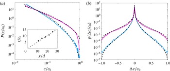
. The concentration PDFs measured at different distances from the source are shown in figure 3.
(a) Concentration PDFs measured at different distances from the source,
 $x/d=10.7$
(blue full line), and
 $x/d=21.4$
(purple full line), for a freely dispersing mixture as in Duplat et al. (Reference Duplat, Innocenti and Villermaux2010). The dashed lines show the predictions of (3.14), with
 $\tilde{t}$
as a unique parameter. The inset shows the fitted values of
 $\tilde{t}$
, which increase linearly as a function of the distance from the injection as expected from (3.15). (b) Concentration increment PDFs measured at the same downstream distances for a spatial increment
 $\unicode[STIX]{x0394}x=50\unicode[STIX]{x1D702}$
. The estimation of the increment PDF from the convolution of independent concentration levels (2.2) is shown as dashed lines.

3.1 Scalar field correlation length under stretching and diffusion
The characteristic correlation length of the scalar field
 $\unicode[STIX]{x1D702}$
is equal here to the average sheet width
 $s$
. Scalar sheets are elongated, in the mean, in two directions with an average elongation
 $\unicode[STIX]{x1D70C}$
such that
 $$\begin{eqnarray}\unicode[STIX]{x1D70C}=1+\unicode[STIX]{x1D70E}_{e}t,\end{eqnarray}$$
where
 $\unicode[STIX]{x1D70E}_{e}$
is the mean elongation rate, given by the velocity difference in the flow at the source scale,
 $\unicode[STIX]{x1D70E}_{e}\sim u/d$
, where
 $u$
is the mean velocity at the source (Duplat et al.
Reference Duplat, Innocenti and Villermaux2010). As a result, the sheets are compressed at a rate
 $\unicode[STIX]{x1D6FE}_{c}=-\langle (1/\unicode[STIX]{x1D70C}^{2})(\text{d}\unicode[STIX]{x1D70C}^{2}/\text{d}t)\rangle$
given by
 $$\begin{eqnarray}\unicode[STIX]{x1D6FE}_{c}=-\frac{2\,\unicode[STIX]{x1D70E}_{e}}{1+\unicode[STIX]{x1D70E}_{e}t}.\end{eqnarray}$$
The sheet width (initially equal to
 $s_{0}$
) evolves through the competition between diffusive broadening and compression in the direction perpendicular to the local elongation as
 $$\begin{eqnarray}\frac{1}{s}\frac{\text{d}s}{\text{d}t}=\frac{D}{s^{2}}+\unicode[STIX]{x1D6FE}_{c}.\end{eqnarray}$$
The mixing time
 $t_{s}$
, corresponding to the time when diffusive broadening
 $D/s^{2}$
equilibrates substrate compression
 $\unicode[STIX]{x1D6FE}_{c}$
, occurs for a dissipation scale
 $s(t_{s})$
such that (Duplat et al.
Reference Duplat, Innocenti and Villermaux2010)
 $$\begin{eqnarray}t_{s}\sim \frac{1}{\unicode[STIX]{x1D70E}_{e}}\left(\frac{\unicode[STIX]{x1D70E}_{e}s_{0}^{2}}{D}\right)^{1/5}\quad \text{and}\quad s(t_{s})\sim s_{0}\left(\frac{\unicode[STIX]{x1D70E}_{e}s_{0}^{2}}{D}\right)^{-2/5}.\end{eqnarray}$$
The temporal behaviour of the sheet width is, for
 $t<t_{s}$
,
 $$\begin{eqnarray}s(t)\sim \frac{s_{0}}{(1+\unicode[STIX]{x1D70E}_{e}t)^{2}}\end{eqnarray}$$
and, for
 $t>t_{s}$
,
 $$\begin{eqnarray}s(t)\sim \sqrt{Dt}.\end{eqnarray}$$
Since stretching rates, and therefore mixing times, are distributed, so are sheet widths (figure 2 a). While strongly stretched sheets reach the mixing scale quickly, those that are stretched at slower rate remain in the first regime for a long time. The mean correlation length is equal to the mean sheet width,
 $$\begin{eqnarray}\unicode[STIX]{x1D702}(t)=\langle s(t)\rangle .\end{eqnarray}$$
For the experiments discussed in this section, the mixing time is reached at a downstream distance of approximately
 $x=2d$
(see inset of figure 3
a). The mixing scale at this distance is approximately
 $s(t_{s})\approx 4~\unicode[STIX]{x03BC}\text{m}$
, and then increases by diffusion, reaching approximately
 $7~\unicode[STIX]{x03BC}\text{m}$
at a distance of
 $x=20d$
.
3.2 Concentration PDFs
Following the approach of Ranz (Reference Ranz1979), the concentration distribution across a stretched lamella can be estimated by assuming that concentration gradients are negligible in the direction of the lamella elongation such that diffusion acts effectively in the direction perpendicular to the lamella elongation. In this direction, the concentration field is subject to a compression rate
 $\unicode[STIX]{x1D6FE}_{c}$
, which compensates the elongation in the other direction for incompressible fluids. Hence, in the Lagrangian frame attached to the lamella, the concentration of a stretched scalar sheet
 $c(\unicode[STIX]{x1D701},t)$
at a position
 $\unicode[STIX]{x1D701}$
along the direction perpendicular to the sheet is
 $$\begin{eqnarray}\frac{\unicode[STIX]{x2202}c}{\unicode[STIX]{x2202}t}=-\unicode[STIX]{x1D6FE}_{c}\unicode[STIX]{x1D701}\frac{\unicode[STIX]{x2202}c}{\unicode[STIX]{x2202}\unicode[STIX]{x1D701}}+D\frac{\unicode[STIX]{x2202}^{2}c}{\unicode[STIX]{x2202}\unicode[STIX]{x1D701}^{2}},\end{eqnarray}$$
where the first term on the right-hand side quantifies compression in the direction perpendicular to the direction of elongation and
 $D$
is the diffusion coefficient. This approach has been shown to describe accurately the evolution of concentration fields under different stretching dynamics, ranging from algebraic to exponential (Duplat et al.
Reference Duplat, Innocenti and Villermaux2010; Meunier & Villermaux Reference Meunier and Villermaux2010).
To solve this equation, we approximate the initial concentration across the sheet by a top-hat profile of width
 $2s_{0}$
, that is
 $c(\unicode[STIX]{x1D701},t=0)=c_{0}H(s_{0}-|\unicode[STIX]{x1D701}|)$
, with
 $H(\unicode[STIX]{x1D701})$
the Heaviside step function. Thus, we have at later times (Ranz Reference Ranz1979; Duplat et al.
Reference Duplat, Innocenti and Villermaux2010; Meunier & Villermaux Reference Meunier and Villermaux2010)
 $$\begin{eqnarray}c(\unicode[STIX]{x1D701},t)=\frac{c_{0}}{2}\left[\text{erf}\left(\frac{s_{0}-\unicode[STIX]{x1D701}}{s_{0}\sqrt{4\unicode[STIX]{x1D70F}}}\right)+\text{erf}\left(\frac{s_{0}+\unicode[STIX]{x1D701}}{s_{0}\sqrt{4\unicode[STIX]{x1D70F}}}\right)\right],\end{eqnarray}$$
where
 $$\begin{eqnarray}\unicode[STIX]{x1D70F}=D\int _{0}^{t}\frac{\text{d}t^{\prime }}{s(t^{\prime })^{2}}.\end{eqnarray}$$
Thus, we obtain for the maximum concentration within the sheet
 $$\begin{eqnarray}c_{m}=c_{0}\text{erf}\left(\frac{1}{\sqrt{4\unicode[STIX]{x1D70F}}}\right).\end{eqnarray}$$
For a linear elongation process in two directions leading to a compression rate decaying in time according to (3.2), expression (3.11) may be approximated by
 $$\begin{eqnarray}c_{m}\approx c_{0}/2(1-\exp [-(t_{s}/t)^{\unicode[STIX]{x1D708}}/\sqrt{\unicode[STIX]{x03C0}}]),\end{eqnarray}$$
with
 $\unicode[STIX]{x1D708}=5/2$
. The sheet concentration goes towards
 $c_{0}$
for
 $t\ll t_{s}$
and
 $c\rightarrow c_{0}(t/t_{s})^{-\unicode[STIX]{x1D708}}/\sqrt{\unicode[STIX]{x03C0}}$
when
 $t\gg t_{s}$
. The mixing time
 $t_{s}$
is distributed around a mean value
 $\langle t_{s}\rangle$
. For a plume released in a turbulent jet, it has been found that the elongation rates are distributed amongst the sheets, but that each of them remains constant in time. Mixing times are exponentially distributed (Duplat et al.
Reference Duplat, Innocenti and Villermaux2010)
 $$\begin{eqnarray}p_{m}(t_{s})=\exp (-t_{s}/\langle t_{s}\rangle )/\langle t_{s}\rangle ,\end{eqnarray}$$
with
 $\langle t_{s}\rangle$
the average mixing time set equal to (3.4). The concentration content of the mixture can be well described by the distribution of maximum concentrations across sheets. Thus the global concentration PDF is obtained from the map (3.12) from the PDF (3.13) of mixing times
 $$\begin{eqnarray}p_{c}(c,\tilde{t})=\frac{\tilde{t}[-\log (1-2c/c_{0})]^{(1/\unicode[STIX]{x1D708})-1}\exp (-\tilde{t}[-\log (1-2c/c_{0})]^{1/\unicode[STIX]{x1D708}})}{(1-2c/c_{0})\unicode[STIX]{x1D708}}\end{eqnarray}$$
valid for
 $0<c<c_{0}$
, and zero else; we define
 $\tilde{t}$
 $$\begin{eqnarray}\tilde{t}=\frac{t}{\langle t_{s}\rangle }\unicode[STIX]{x03C0}^{1/2\unicode[STIX]{x1D708}}=\frac{x}{u\langle t_{s}\rangle }\unicode[STIX]{x03C0}^{1/2\unicode[STIX]{x1D708}}.\end{eqnarray}$$
This expression quantifies the impact of stretching statistics, reflecting velocity statistics in the turbulent jet, on the distribution of concentrations. The resulting analytical predictions compare well with the experimental data (figure 3
a), providing an accurate estimate of the full PDF of concentrations at any position downstream of the dye injection location. As shown in the inset of figure 3(a), these predictions are obtained with a unique parameter
 $\tilde{t}$
, which increases linearly with the distance from the injection as expected from (3.15).
After the mixing time, the average sheet concentration decays as
 $$\begin{eqnarray}\langle c\rangle \propto (t/\langle t_{s}\rangle )^{-5/2},\end{eqnarray}$$
a scaling which can be understood as resulting from the distribution of the sheet mass over a volume that increases linearly in two elongation directions in the sheet plane and diffusively in the direction normal to the sheet plane.
3.3 Concentration increment PDFs
We now examine the shape and evolution of concentration increment PDFs, which have not been analysed by Duplat et al. (Reference Duplat, Innocenti and Villermaux2010). Since the jet is freely dispersing, sheets are distant from each other and undergo minimum aggregation. Note that some isolated diffusive coalescence events do occur, as illustrated in figure 2(a). However, these events do not significantly affect the concentration statistics, which are well predicted by (3.14), which assumes that sheets are independent. Hence, for spatial increments
 $\unicode[STIX]{x0394}x$
larger than the correlation scale
 $\unicode[STIX]{x1D702}$
(3.7), the PDF of concentration increments is obtained by inserting the analytical expression derived for the concentration PDF (3.14) into the self-convolution equation (2.2). This convolution can be written as
 $$\begin{eqnarray}p_{\unicode[STIX]{x1D6E5}}(\unicode[STIX]{x0394}c)=\int _{0}^{\infty }\,\text{d}z\tilde{t}\exp (-z\tilde{t})p_{c}(c_{0}[1-\exp (-z^{\unicode[STIX]{x1D708}})]+|\unicode[STIX]{x0394}c|).\end{eqnarray}$$
Using the sharp decay of the exponential for
 $z>1/\tilde{t}$
, we may approximate
 $\tilde{t}\,\exp (-z\tilde{t})\approx \unicode[STIX]{x1D6FF}(z)/2$
such that
 $$\begin{eqnarray}p_{\unicode[STIX]{x1D6E5}}(\unicode[STIX]{x0394}c)\approx {\textstyle \frac{1}{2}}p_{c}(|\unicode[STIX]{x0394}c|).\end{eqnarray}$$
As shown by this approximation, the PDFs of concentration increments are very close to the PDFs of concentrations themselves. This is expected since the PDF of concentrations is sharply peaked around zero (figure 3
b), which implies that most concentration increments result from the difference between a given concentration value
 $c_{1}$
close to a sheet centre and a small concentration pertaining to diffusive profiles far from the sheet centre
 $c_{2}\ll c_{1}$
, such that
 $\unicode[STIX]{x0394}c=c_{1}-c_{2}\approx c_{1}$
: convolution with a Dirac delta at the origin preserves the original distribution (see figure 1
d).
As for the concentration PDFs, the concentration increment PDFs reflect the distribution of stretching rates resulting from velocity statistics in the turbulent jet. The predictions obtained from (3.18) compare well with experimental measurements, providing an accurate estimate of concentration increment PDFs at different downstream locations from the source. These predictions are made with no fitting parameters, since
 $\unicode[STIX]{x1D708}=5/2$
and
 $\tilde{t}$
is set from the concentration PDF analysis (see inset of figure 3
a) in agreement with (3.15). Here we consider spatial increments larger than the correlation scale
 $\unicode[STIX]{x0394}x>\unicode[STIX]{x1D702}$
, since the average mixing scale
 $\unicode[STIX]{x1D702}$
is very small in the considered experiment (approximately
 $5{-}7~\unicode[STIX]{x03BC}\text{m}$
from (3.4)).
Note that a similar result was obtained by Le Borgne et al. (Reference Le Borgne, Dentz and Villermaux2015) for low-Reynolds-number porous media flows at high Peclet numbers, whose velocity distribution differs strongly from that of turbulent flows. Although the equation describing concentration increments in this context is different from (3.17), because the stretching rate distribution is fundamentally different, the basic argument for deriving concentration increments is similar. This suggests a broad generality of the proposed concentration increment theory for a range of velocity fields. In the following, we explore concentration increment PDFs in turbulent mixtures undergoing significant self-aggregation.
4 Fully developed aggregation in confined turbulent jets
The dispersing mixtures studied in the previous section represents a case of minimum aggregation; we now consider the opposite scenario of fully developed aggregation. For this we analyse the experimental data set of Duplat & Villermaux (Reference Duplat and Villermaux2008), which is similar to that described above except that a duct is included for confining the turbulent jet. The confinement thus maximizes the sheet aggregation process. Duplat & Villermaux (Reference Duplat and Villermaux2008) showed that concentration PDFs are correctly described by a self-convolution process, which we recall briefly here for completeness. We then analyse the shape and evolution of concentration increment PDFs within the theoretical framework presented in § 2.3.
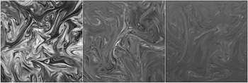
Figure 2(b) shows how the dye rapidly invades the whole cross-section of the duct, and how its concentration differences are progressively erased while travelling downstream to relax towards a more or less uniform mixture. As for the freely dispersing jet, the flow disorder creates scalar sheets elongating in time and occupying more and more space in the duct. The confinement favours scalar sheets coalescence and gives rise to new sheets whose concentration profile is the addition of the original ones (figure 4). The average concentration of the mixture
 $\langle c\rangle$
is conserved.
Mixing of a dye discharging from a jet of diameter
 $d=8~\text{mm}$
in a square (
 $L\times L$
with
 $L=3~\text{cm}$
) duct. The figure shows successive instantaneous planar cuts of the scalar field at increasing downstream locations in the duct, showing the progressive uniformization of the dye concentration levels; from Duplat & Villermaux (Reference Duplat and Villermaux2008).

4.1 Concentration PDF
Assuming that the aggregating sheets have independent stretching histories, diffusive coalescence can be described as a random aggregation process (Villermaux & Duplat Reference Villermaux and Duplat2003). This can be formalized by a general equation for the concentration PDF that quantifies its evolution through self-convolution and stretching-enhanced diffusion (Duplat & Villermaux Reference Duplat and Villermaux2008). The solution of this equation is a family of gamma distributions:
 $$\begin{eqnarray}p_{c}(c/\langle c\rangle ,t)=\frac{n^{n}}{\unicode[STIX]{x0393}(n)}\left(\frac{c}{\langle c\rangle }\right)^{n-1}\exp \left(-n\frac{c}{\langle c\rangle }\right),\end{eqnarray}$$
where
 $n$
is the average number of aggregations, which is such that it restores, by addition, the average mixture concentration
 $\langle c(\boldsymbol{x},t)\rangle$
 $$\begin{eqnarray}\langle c(\boldsymbol{x},t)\rangle =n(t)\unicode[STIX]{x1D703}(t),\end{eqnarray}$$
where
 $\unicode[STIX]{x1D703}(t)$
is the average concentration of an elementary sheet at time
 $t$
, which results from the stretching-enhanced diffusive regime described previously (3.16). Since the average concentration is constant in this experiment, and since
 $\unicode[STIX]{x1D703}\sim t^{-\unicode[STIX]{x1D708}}$
, the expected scaling of the average coalescence number is (Duplat & Villermaux Reference Duplat and Villermaux2008)
 $$\begin{eqnarray}n(t)\sim \left(\frac{t}{\langle t_{s}\rangle }\right)^{\unicode[STIX]{x1D708}},\end{eqnarray}$$
with
 $\unicode[STIX]{x1D708}=5/2$
. As shown by Duplat & Villermaux (Reference Duplat and Villermaux2008), and illustrated in figure 5(b), concentration distributions in this regime are well described by the predictions of (4.1), thus confirming the validity of the random aggregation model. These gamma distributions are defined by a single parameter
 $n(t)$
, which increases in time according to (4.3). Therefore, in this regime, the statistics of concentrations are no longer determined by the distribution of stretching rates, as described in the previous section, but by the frequency of lamella aggregation, quantified by
 $n(t)$
.
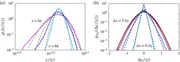
Comparison of measured and predicted concentration distributions and concentration increment distributions for the confined turbulent mixture. (a) Concentration PDFs measured at different distances (
 $4L$
,
 $5L$
,
 $6L$
) from the source (full lines) and predicted from gamma distributions of order
 $n=\{20,35,95\}$
(dashed lines), (b) Concentration increment PDFs at
 $x=4L$
measured for different spatial increments
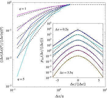
 $\unicode[STIX]{x0394}x=\{0.2\unicode[STIX]{x1D702},0.7\unicode[STIX]{x1D702},2.5\unicode[STIX]{x1D702},3.5\unicode[STIX]{x1D702}\}$
(full lines) and predicted by (4.5) (dashed lines).

4.2 Coarse graining scale
The aggregation process results in the creation of sheet bundles of characteristic size
 $\unicode[STIX]{x1D702}=ns$
, where
 $s$
is the average sheet width, which evolves through stretching and diffusion (3.3). The correlation scale
 $\unicode[STIX]{x1D702}$
, also called the coarse graining scale (Villermaux & Duplat Reference Villermaux and Duplat2006), is thus much larger than the characteristic sheet scale
 $s$
. From the temporal evolution of
 $n(t)$
in (4.3) and of
 $s(t)$
in (3.6), the coarse graining scale is expected to scale as
 $$\begin{eqnarray}\unicode[STIX]{x1D702}(t)\sim \sqrt{D\langle t_{s}\rangle }\left(\frac{t}{\langle t_{s}\rangle }\right)^{\unicode[STIX]{x1D708}+1/2}.\end{eqnarray}$$
In a confined domain, this rapid growth is similar to a percolation process (Villermaux Reference Villermaux2012a
; Le Borgne et al.
Reference Le Borgne, Dentz and Villermaux2015) and, at the percolation threshold, the correlation length is a fraction of the domain size. For the confined jet experiment,
 $\unicode[STIX]{x1D702}$
varies from
 $\unicode[STIX]{x1D702}=0.9~\text{mm}$
at a distance from the duct inlet
 $x=4L$
, to
 $\unicode[STIX]{x1D702}=2.7~\text{mm}$
at
 $x=6L$
.
4.3 Concentration increment PDFs
Based on the earlier results for concentration PDFs recalled above and the general framework presented in § 2.3, we now analyse the shape and evolution of concentration increment PDFs. Under random aggregation, concentration fields develop complex spatial correlation patterns, which are induced by multiple interactions between sheets (figure 1
a). As demonstrated in § 2.3, differences in neighbouring concentration levels are expected to depend only on the sheets that have aggregated independently at the two locations, while the contribution of common aggregated sheets is eliminated by the difference operator (figure 1
c). This principle leads to a closed-form expression for the concentration increment PDF (5.8). Inserting (4.1) into this equation, we obtain the following expression for the concentration increment PDF for the confined turbulent jet, where
 $\text{K}_{p}(\cdot )$
denotes the modified Bessel function of the second kind of order
 $p$
(Abramowitz & Stegun Reference Abramowitz and Stegun1964)
 $$\begin{eqnarray}p_{\unicode[STIX]{x0394}x<\unicode[STIX]{x1D702}}(\unicode[STIX]{x0394}c)=\frac{1}{\sqrt{\unicode[STIX]{x03C0}}\unicode[STIX]{x1D703}^{2m(\unicode[STIX]{x0394}x)}\unicode[STIX]{x0393}(m(\unicode[STIX]{x0394}x))}\left(\frac{|\unicode[STIX]{x0394}c|\unicode[STIX]{x1D703}}{2}\right)^{m(\unicode[STIX]{x0394}x)-1/2}\text{K}_{m(\unicode[STIX]{x0394}x)-1/2}\left(\frac{|\unicode[STIX]{x0394}c|}{\unicode[STIX]{x1D703}}\right).\end{eqnarray}$$
This expression depends on two parameters: the mean sheet concentration
 $\unicode[STIX]{x1D703}(t)$
, given by (3.12), and the number of independent sheets
 $m(\unicode[STIX]{x0394}x)$
, given by (2.12). For
 $\unicode[STIX]{x0394}x>\unicode[STIX]{x1D702}$
, the increment PDF is expected to be invariant with
 $\unicode[STIX]{x0394}x$
, since all possible concentration differences have been sampled (see figure 5
b). This property is expressed by the convergence of
 $m(\unicode[STIX]{x0394}x)$
to
 $n(t)$
((2.12) and figure 6). Note that the shape of the concentration increment PDFs differs from those observed for the dispersing mixture, which are sharply peaked around zero (figure 3
b). The latter is mostly related to the existence of diffusive tails around sheets that lead to large probabilities for low concentration levels. The absence of a sharp peak around zero in the confined mixture (figure 5
b) is thus a manifestation of the fully developed aggregation process that fills the diffusive profiles in between the sheets. As discussed in the next section, this is not the case for partial aggregation regimes where material lines are non-space-filling.
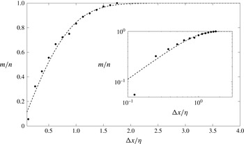
Number of independent sheets
 $m$
participating in concentration increments as a function of the spatial increment
 $\unicode[STIX]{x0394}x$
for the confined mixture at a distance
 $x=4L$
. This number is obtained by fitting (4.5) to the concentration increment PDFs of figure 5(b). Inset: same in log–log plot. The dashed line represents the prediction of (2.12).

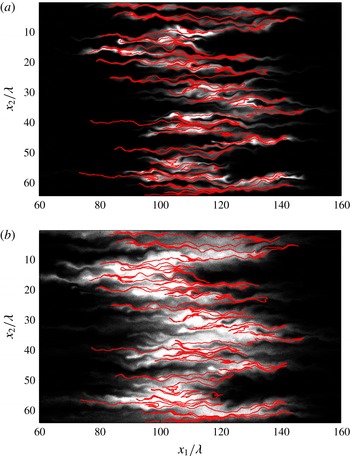
Snapshot of concentration field simulated in a heterogeneous porous medium, with permeability field variance
 $\unicode[STIX]{x1D70E}_{\ln K}^{2}=1$
and Peclet number (a)
 $Pe=800$
and (b)
 $Pe=80$
. The colour scale is the same as in figure 2. The concentration field is normalized by its maximum value. The superposition of a purely advected line (in red) illustrates the construction of the scalar mixture from an ensemble of lamellae experiencing distributed stretching rates in (a) and random aggregation in (b).

The predictions of (4.5) are in good agreement with the measured concentration increment PDFs measured for different spatial increments
 $\unicode[STIX]{x0394}x$
(figure 5
b). Since the temporal evolution of the mean sheet concentration
 $\unicode[STIX]{x1D703}(t)$
is known from the analysis of the freely dispersing jet in the previous sections (3.12), these predictions are obtained with a single parameter
 $m(\unicode[STIX]{x0394}x)$
. The evolution of the number of independent
 $m(\unicode[STIX]{x0394}x)$
with the spatial increment is consistent with the prediction of (2.12) (figure 6). For small spatial increments
 $\unicode[STIX]{x0394}x$
, the number of independent sheets participating in concentration levels at neighbouring locations tends to zero, while at large spatial increments it tends to
 $n$
and becomes independent of
 $\unicode[STIX]{x0394}x$
. Hence, spanning through the spatial increments is equivalent to deconstructing the different stages of aggregation from the elementary sheet stage for
 $m\rightarrow 0$
to the fully developed aggregation stage for
 $m\rightarrow n$
. The key parameter quantifying the spatial structure of mixtures is
 $m(\unicode[STIX]{x0394}x)$
, measuring the density of material lines as a function of scale, which dictates the progress of aggregation as the diffusion scale increases (2.12). Consistently, its cross-over towards saturation at
 $m=n$
occurs for
 $\unicode[STIX]{x0394}x$
of the order of
 $\unicode[STIX]{x1D702}$
.
Note that expression (4.5) is similar to the result previously obtained for concentration increments in porous media flows at low Peclet numbers (Le Borgne et al.
Reference Le Borgne, Dentz and Villermaux2015). While concentration increment PDFs in these two flow systems obey the same general law, despite having markedly distinct velocity distributions, they differ in the temporal scaling of the mean sheet concentration
 $\unicode[STIX]{x1D703}(t)$
and the spatial scaling of the density of independent sheets
 $m(\unicode[STIX]{x0394}x)$
, which are the two parameters determining how the shape of concentration increment PDFs evolve with time and spatial increment. These two parameters thus quantify the impact of the velocity distribution on the increment PDFs. The temporal decay of the mean sheet concentration
 $\unicode[STIX]{x1D703}(t)$
depends on the stretching dynamics:
 $\unicode[STIX]{x1D703}\sim t^{-5/2}$
for the considered turbulent jet and
 $\unicode[STIX]{x1D703}\sim t^{-\unicode[STIX]{x1D6FC}}$
, with
 $1<\unicode[STIX]{x1D6FC}<5/2$
, for two-dimensional porous media. On the other hand, the increase of the number of independent sheets with spatial increment
 $m(\unicode[STIX]{x0394}x)$
is controlled by the fractal dimension of purely advected material lines (2.11). The latter depends on the relative importance of stretching and dispersion. While stretching tends to fill space with material lines, dispersion increases the global area that they occupy. In the case of confined turbulent jet, the presence of the duct prevents lateral spreading. The stretched sheets hence rapidly become space filling (see figures 3
b and 4). In porous media, however, persistent flow heterogeneities prevent material lines from filling the domain (see red lines in figure 7). In other words, the stretching dynamics are not fast enough to fill the domain created by dispersion. For two-dimensional porous media, this has been shown to lead to a stable fractal dimension,
 $1<d_{f}<2$
(Le Borgne et al.
Reference Le Borgne, Dentz and Villermaux2015). This has important consequences for the development of intermittency, as discussed in the following section.
5 Partial aggregation and intermittency
The previous sections have discussed two scenarios of minimum and maximum aggregation. In general, heterogeneous flows lie in between these extreme situations. In particular, dense lamella aggregates have been shown to coexist with concentration lacunarities in flow fields characterized by a broad distribution of velocities that produce non-space-filling material lines (Le Borgne et al.
Reference Le Borgne, Dentz and Villermaux2013). Porous media flows pertain to this category, as strong spatial fluctuations in permeability produce complex mixing patterns, which control chemical reactions in a range of applications, including
 $\text{CO}_{2}$
sequestration, soil remediation, geothermal systems and enhanced oil recovery (Battiato et al.
Reference Battiato, Tartakovsky, Tartakovsky and Scheibe2009; Bijeljic, Mostaghimi & Blunt Reference Bijeljic, Mostaghimi and Blunt2011; Dentz et al.
Reference Dentz, LeBorgne, Englert and Bijeljic2011; Chiogna et al.
Reference Chiogna, Hochstetler, Bellin, Kitanidis and Rolle2012; Engdahl, Bolster & Benson Reference Engdahl, Bolster and Benson2014; Hidalgo et al.
Reference Hidalgo, Dentz, Cabeza and Carrera2015; Jimenez-Martinez et al.
Reference Jimenez-Martinez, Porter, Hyman, Carey and Viswanathan2016). As discussed in the previous section, for the cases of very large and very low Peclet numbers, concentration increment PDFs may be described in the same general theory with respectively limited lamella interaction or fully developed aggregation (Le Borgne et al.
Reference Le Borgne, Dentz and Villermaux2015). Yet, the applications mentioned above lead to a broad range of Peclet numbers, for which these extreme scenarios do not apply. Here we investigate the shape and temporal evolution of concentration increments in the case of intermediate Peclet number, which may be relevant for a class of applications.
Figure 7 shows a snapshot of a stretched material line, and of the associated concentration field, in a two-dimensional incompressible flow through a heterogeneous porous media (Le Borgne et al.
Reference Le Borgne, Dentz and Villermaux2015). The conductivity
 $K(\boldsymbol{x})$
is represented as a lognormally distributed random field, such as
 $f(\boldsymbol{x})=\ln K(\boldsymbol{x})$
is normally distributed with mean
 $\overline{f}=1$
, variance
 $\unicode[STIX]{x1D70E}_{f}^{2}=1$
and correlation length
 $\unicode[STIX]{x1D706}$
. This type of random conductivity is generic and represents a reference field for theories of flow and transport in heterogeneous porous media. Spatial variability in conductivity
 $K(\boldsymbol{x})$
leads to spatial fluctuations in the divergence-free flow field
 $\boldsymbol{u}(\boldsymbol{x})$
via the Darcy equation
 $\boldsymbol{u}(\boldsymbol{x})=-K(\boldsymbol{x})\unicode[STIX]{x1D735}h(\boldsymbol{x})$
, with
 $h(\boldsymbol{x})$
the hydraulic head. Flow is driven by a mean pressure gradient from left to right. It is confined by impermeable horizontal boundaries at the bottom and the top. The initial condition is given by an instantaneous uniform line injection at
 $x_{1}=\unicode[STIX]{x1D706}$
. The characteristic advection time scale is defined by
 $\unicode[STIX]{x1D70F}_{a}=\unicode[STIX]{x1D706}/\overline{u}$
, where
 $\overline{u}$
is the mean transport velocity. The characteristic diffusion time is
 $\unicode[STIX]{x1D70F}_{D}=\unicode[STIX]{x1D706}^{2}/D$
. The Péclet number
 $$\begin{eqnarray}Pe=\frac{\unicode[STIX]{x1D706}\overline{u}}{D}\end{eqnarray}$$
compares the diffusive and advective time scales.
As illustrated in figure 7, Darcy flows generate a heterogeneous spatial distribution of lamella density (purely advected red lines) with areas focusing a large number of lamellae next to empty regions. This spatial structure can be quantified by the material line fractal dimension. For the considered flow field
 $d_{f}=1.6$
has been shown to be stationary in time. This stable fractal dimension results from power-law scaling behaviours of the dispersion length and the line elongation, which are both linked to the existence of broad velocity distributions (Le Borgne et al.
Reference Le Borgne, Dentz and Villermaux2013). Figure 7(a) shows the initiation of aggregation at Peclet
 $Pe=800$
, where the shape of lamellae that develop around the material lines are still distinguished. As more and more lamellae merge, concentration fields can be viewed as an ensemble of lamellae bundles separated by concentration lacunarities (figure 7
b). Although the shapes of lamellae are no longer apparent in the concentration field, the number of underlying lamellae in each bundle can be visualized from the superimposed purely advected material lines (in red) obtained from the numerical simulation. While stretched lamellae are not directly visible in the concentration field, their continuous aggregation still controls the concentration statistics. In particular, large concentrations are found in areas of dense lamella aggregation.
5.1 Concentration PDF
Before analysing concentration increments, we recall previous results obtained for concentration PDFs for the regime of partial aggregation (Le Borgne et al.
Reference Le Borgne, Dentz and Villermaux2015). In this regime, the statistics of concentrations have been shown to be well described by approximating the concentration profiles
 $c^{\prime }(\boldsymbol{x},t)$
around aggregates as Gaussian spatial profiles whose maximum concentration evolves through a random aggregation process. The statistics of local concentration maxima are thus expected to follow gamma distributions, as described in the previous section (4.1). The concentration profiles around each maximum, which develop towards the concentration lacunarities, introduce an additional variability in concentrations that can be quantified by the concentration PDF of a Gaussian function conditional to its maximum (Le Borgne et al.
Reference Le Borgne, Dentz and Villermaux2015),
 $$\begin{eqnarray}p_{c}(c\mid c_{max})=\frac{1}{2c\sqrt{\ln (c_{max}/\unicode[STIX]{x1D716})\ln (c_{max}/c)}},\end{eqnarray}$$
where
 $\unicode[STIX]{x1D716}$
is the minimum concentration that is required for normalization. This conditional PDF quantifies in particular the large probability associated with low concentration values, with a typical scaling
 $p_{c}(c)\sim 1/c$
when
 $c\rightarrow 0$
. This scaling, associated with diffusion profiles, is not found in the fully developed aggregation scenario previously described, since aggregation prevents these profiles to develop. On the other hand, the presence of concentration lacunarities allows the existence of diffusive tails around lamellae aggregates. With the gamma distribution for local concentration maxima, the global concentration PDF
 $p_{c}(c)$
is thus (Le Borgne et al.
Reference Le Borgne, Dentz and Villermaux2015)
 $$\begin{eqnarray}p_{c}(c\mid n)=\int _{c}^{\infty }\,\text{d}x\frac{x^{n-1}}{\unicode[STIX]{x0393}(n)\unicode[STIX]{x1D703}^{n}}\frac{\exp (-x/\unicode[STIX]{x1D703})}{2c\sqrt{\ln (x/\unicode[STIX]{x1D716})\ln (x/c)}},\end{eqnarray}$$
where, as for (4.1),
 $n$
is the average number of aggregation and
 $\unicode[STIX]{x1D703}$
is the mean lamella concentration.
From the analysis of the stretching statistics in the considered porous media, the elongation distribution was found to be well modelled by a multiplicative process leading to a lognormal elongation distribution of average
 $\langle \log \unicode[STIX]{x1D70C}\rangle \sim \unicode[STIX]{x1D707}_{1}\log (t/\unicode[STIX]{x1D70F}_{a})$
and variance
 $\unicode[STIX]{x1D70E}_{\log \unicode[STIX]{x1D70C}}^{2}\sim 2\unicode[STIX]{x1D707}_{2}\log (t/\unicode[STIX]{x1D70F}_{a})$
. This leads to a power-law increase of the mean elongation as
 $\langle \unicode[STIX]{x1D70C}\rangle \sim t^{\unicode[STIX]{x1D707}_{1}+\unicode[STIX]{x1D707}_{2}}$
, and accordingly to a power-law decay of the mean lamella concentration such as
 $$\begin{eqnarray}\unicode[STIX]{x1D703}(t)=c_{0}(t/\unicode[STIX]{x1D70F}_{a})^{-\unicode[STIX]{x1D707}_{1}+\unicode[STIX]{x1D707}_{2}-1/2}.\end{eqnarray}$$
For the case studied here (
 $\unicode[STIX]{x1D70E}_{\log K}^{2}=1$
, figure 7), the elongation distribution exponents are
 $\unicode[STIX]{x1D707}_{1}=0.7$
and
 $\unicode[STIX]{x1D707}_{2}=0.2$
(Le Borgne et al.
Reference Le Borgne, Dentz and Villermaux2015). Once
 $\unicode[STIX]{x1D703}$
is determined from the elongation dynamics, the only parameter for the concentration PDFs is the total number of lamella aggregation
 $n$
. The latter may estimated by quantifying the average number of lamellae in a radius of diffusion (Le Borgne et al.
Reference Le Borgne, Dentz and Villermaux2015),
 $$\begin{eqnarray}n(t)\sim \left(\sqrt{Dt}\right)^{d_{f}-d+1},\end{eqnarray}$$
where for the considered two-dimensional porous media the fractal dimension is stable in time and equal to
 $d_{f}=1.6$
.
For
 $c/(n\unicode[STIX]{x1D703})<1$
, equation (5.3) can be approximated by (see appendix B)
 $$\begin{eqnarray}p_{c}(c\mid n)\approx \frac{\sqrt{2\unicode[STIX]{x03C0}(n-1)}\exp [(n-1)\ln [(n-1)]-(n-1)]}{2\unicode[STIX]{x0393}(n)c\sqrt{\ln [(n-1)\unicode[STIX]{x1D703}/\unicode[STIX]{x1D716}]\ln [(n-1)\unicode[STIX]{x1D703}/c]}}\end{eqnarray}$$
while for
 $c/(n\unicode[STIX]{x1D703})>1$
, it may be approximated by
 $$\begin{eqnarray}p_{c}(c\mid n)\approx \frac{c^{n-1}}{2\unicode[STIX]{x1D703}^{n}\unicode[STIX]{x0393}(n)}\frac{\exp (-c/\unicode[STIX]{x1D703})}{\sqrt{\ln (c/\unicode[STIX]{x1D716})}}\frac{\sqrt{\unicode[STIX]{x03C0}/(n-1)}}{\sqrt{c/((n-1)\unicode[STIX]{x1D703})-1}}.\end{eqnarray}$$
The predictions provided by (5.3), where
 $n$
is the only free parameter once
 $\unicode[STIX]{x1D703}$
is determined from the analysis of stretching distribution (5.4), are shown in figure 8(a). As discussed in Le Borgne et al. (Reference Le Borgne, Dentz and Villermaux2015), these predictions are in good agreement with the simulations when
 $n$
increases with time according to (5.5). The behaviour of the concentration PDF for large concentrations is close to a gamma distribution as in the full aggregation regime (4.1), since large concentrations coincide with the maximum concentrations of lamella aggregates, which follow a gamma distribution. This differs from the minimum aggregation regime (see inset of figure 8
a). The behaviour at small concentrations follows a
 $1/c$
scaling characteristic of the diffusive profiles developing in the concentration lacunarities, as for the minimum aggregation scenario (figure 8
a). This introduces a peak of probability at low concentration which has an important impact on the concentration increment PDF and on the scaling of the associated structure functions, as discussed in the following.
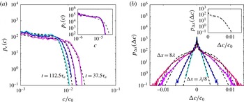
Comparison of analytical predictions of concentration distributions and concentration increment distributions to simulations for a Darcy field with
 $\unicode[STIX]{x1D70E}_{\ln K}^{2}=1$
and Peclet
 $Pe=80$
(see figure 7
b). (a) PDF of concentrations
 $p_{c}(c)$
at times
 $t=37.5\unicode[STIX]{x1D70F}_{a}$
,
 $62.5\unicode[STIX]{x1D70F}_{a}$
,
 $87.5\unicode[STIX]{x1D70F}_{a}$
and
 $112.5\unicode[STIX]{x1D70F}_{a}$
from simulations (full lines) and analytical predictions (dashed lines, equation (5.3)). Inset: concentration PDF at time
 $t=37.5\unicode[STIX]{x1D70F}_{a}$
compared to the prediction of a lamella mixing model (grey dash-dotted line) that neglects aggregation as in § 3. (b) PDF of concentration increments
 $p_{\unicode[STIX]{x0394}x}(\unicode[STIX]{x0394}c)$
at time
 $t=112.5\unicode[STIX]{x1D70F}_{a}$
for
 $\unicode[STIX]{x0394}x=\unicode[STIX]{x1D706}/8$
,
 $\unicode[STIX]{x1D706}/2$
,
 $2\unicode[STIX]{x1D706}$
,
 $8\unicode[STIX]{x1D706}$
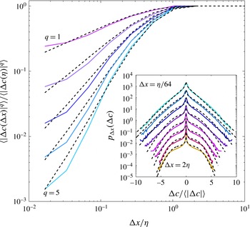
, from simulations (full lines) and analytical predictions (dashed lines, equation (5.9)). Inset: comparison of
 $p_{\unicode[STIX]{x0394}x}(\unicode[STIX]{x0394}c)$
(black dashed line, equation (5.8)) and
 $1/2p_{c}(|\unicode[STIX]{x0394}c|)$
(full grey line, equation (5.9)) for the case corresponding to
 $t=112.5\unicode[STIX]{x1D70F}_{a}$
and
 $\unicode[STIX]{x0394}x=8\unicode[STIX]{x1D706}$
.

5.2 Concentration increment PDFs
We now derive the concentration increment PDFs for the partial aggregation regime. In this regime, the mixture is composed of lamella bundles, which have developed through diffusive aggregation, separated by concentration lacunarities. Applying the principle presented in § 2.3, concentration gradients within lamella bundles are expected to be directly related to the fraction of independent lamellae participating in the value of concentration at neighbouring locations by random aggregation. The number of independent lamellae
 $m(\unicode[STIX]{x0394}x)$
grows with the separation distance, following (2.12). Since material lines are non-space-filling,
 $d_{f}=1.6$
, the growth of
 $m$
with
 $\unicode[STIX]{x0394}x$
is slower than in the fully developed aggregation case. The concentration increment PDF is thus obtained as
 $$\begin{eqnarray}p_{\unicode[STIX]{x0394}x<\unicode[STIX]{x1D702}}(\unicode[STIX]{x0394}c)=\int \,\text{d}c^{\prime }p_{c}(c^{\prime },t\mid m)p_{c}(|\unicode[STIX]{x0394}c|-c^{\prime },t\mid m),\end{eqnarray}$$
where
 $p_{c}(c^{\prime },t\mid m)$
is the concentration PDF corresponding to an aggregation of
 $m$
independent lamellae given in (5.3).
Since the concentration PDFs are sharply peaked around zero (5.6), a significant part of the large concentration increments are obtained by the subtraction from the concentration within a lamella bundle
 $c_{1}$
of a small concentration pertaining to diffusive profiles in lacunarities
 $c_{2}\ll c_{1}$
, such that
 $\unicode[STIX]{x0394}c=c_{1}-c_{2}\approx c_{1}$
. This implies, as in § 3.3, that the concentration increment PDFs are expected to be close to the concentration PDFs themselves:
 $p_{\unicode[STIX]{x0394}x}(\unicode[STIX]{x0394}c)\approx 1/2p_{c}(|\unicode[STIX]{x0394}c|)$
(see inset of figure 8
b),
 $$\begin{eqnarray}p_{\unicode[STIX]{x0394}x<\unicode[STIX]{x1D702}}(\unicode[STIX]{x0394}c)=1/2\int _{|\unicode[STIX]{x0394}c|}^{\infty }\,\text{d}x\frac{x^{n-1}}{\unicode[STIX]{x0393}(m(\unicode[STIX]{x0394}x))\unicode[STIX]{x1D703}^{m(\unicode[STIX]{x0394}x)}}\frac{\exp (-x/\unicode[STIX]{x1D703})}{2|\unicode[STIX]{x0394}c|\sqrt{\ln (x/\unicode[STIX]{x1D716})\ln (x/|\unicode[STIX]{x0394}c|)}},\end{eqnarray}$$
which can be approximated by expressions (5.6) and (5.7). This expression is determined by two parameters:
 $\unicode[STIX]{x1D703}$
and
 $m$
. The mean lamella concentration
 $\unicode[STIX]{x1D703}$
, which is determined by the stretching dynamics coupled to diffusion, is given by (5.4). The number of independent lamella
 $m$
is set by the evolution of lamella density with scale according to (2.12).
The predictions obtained from (5.9) are in good agreement with the simulations (figure 8
b), with the parameter
 $m$
evolving according to (2.12). The shape of the increment PDFs depends on the spatial increment
 $\unicode[STIX]{x0394}x$
, which implies that the increment PDFs cannot be collapsed by rescaling. This property is a characteristic of intermittent processes (e.g. Antonia et al.
Reference Antonia, Hopfinger, Gagne and Anselmet1984; Warhaft Reference Warhaft2000; Falkovich et al.
Reference Falkovich, Gawedzki and Vergassola2001). Intermittency is linked here to the coexistence of densely aggregated lamellae and concentration lacunarities. For small spatial increments
 $\unicode[STIX]{x0394}x$
, the concentration increment PDFs are sharply peaked around zero and decay nearly exponentially for large increments. While the peak around zero corresponds to concentration lacunarities, the exponential decay is the signature of a small aggregation number
 $m$
. Since neighbouring concentration levels have a large number of contributing elementary lamellae in common, their difference is made from a small number of independent lamellae
 $m$
. On the other hand, for large spatial increments
 $\unicode[STIX]{x0394}x$
, the concentration increment PDFs are still sharply peaked around zero, owing to concentration lacunarities, but the decay at large concentration increments is no longer exponential. The latter converges to a gamma distribution of order
 $m\rightarrow n$
as
 $\unicode[STIX]{x0394}x\rightarrow \unicode[STIX]{x1D702}$
, as predicted from our framework. Hence the shapes of the increment PDFs for different spatial increments reveal the different stages of aggregation that have occurred to determine the current structure of scalar fields, while only the largest stage of aggregation
 $m=n$
is visible in the field concentration PDF. Note that the evolution of
 $m$
with
 $\unicode[STIX]{x0394}x$
is dictated by the fractal dimension of purely advected material lines
 $d_{f}$
according to (2.12). This quantifies the dependency of concentration increments on the velocity statistics, which determines
 $d_{f}$
(Villermaux Reference Villermaux2012b
). Consequences for the scaling of structure functions are discussed in the following section.
6 Structure functions and intermittency
A surrogate of the full PDF of increments is the hierarchy of its moments
 $q$
, also called the structure functions when their scaling dependence on
 $\unicode[STIX]{x0394}x$
is studied
 $$\begin{eqnarray}\langle |\unicode[STIX]{x0394}c|^{q}\rangle =\int \,\text{d}\unicode[STIX]{x0394}c|\unicode[STIX]{x0394}c|^{q}p_{\unicode[STIX]{x0394}x}(\unicode[STIX]{x0394}c).\end{eqnarray}$$
Structure functions typically increase with
 $\unicode[STIX]{x0394}x$
, as correlation between concentrations
 $c(\boldsymbol{x},t)$
and
 $c(\boldsymbol{x}+\unicode[STIX]{x0394}\boldsymbol{x},t)$
decreases and larger increments
 $c(\boldsymbol{x}+\unicode[STIX]{x0394}\boldsymbol{x},t)-c(\boldsymbol{x},t)$
are sampled. For spatial increments larger than the correlation length
 $\unicode[STIX]{x1D702}$
, structure functions are expected to reach a plateau when all possible concentration differences have been sampled.
The scaling of structure functions with
 $\unicode[STIX]{x0394}x$
has been analysed to characterize the spatial structure of scalar fields in a range of flows (Warhaft Reference Warhaft2000). Anomalous scaling behaviours have been referred to as a manifestation of intermittent properties of scalar fields. Intermittency has been characterized in particular by a nonlinear dependency of scaling exponents
 $\unicode[STIX]{x1D709}(q)$
on the order
 $q$
, where
 $\unicode[STIX]{x1D709}(q)$
is such that
 $\langle |\unicode[STIX]{x0394}c|^{q}\rangle \sim \unicode[STIX]{x0394}x^{\unicode[STIX]{x1D709}(q)}$
. These anomalous scaling behaviour are generally associated with an evolution with
 $\unicode[STIX]{x0394}x$
of the shape of increment PDFs, which cannot be collapsed upon rescaling with
 $\langle |\unicode[STIX]{x0394}c|\rangle$
, or with
 $\sqrt{\langle \unicode[STIX]{x0394}c^{2}\rangle }$
. The scaling of structure functions with
 $\unicode[STIX]{x0394}x$
naturally derives from the theory developed above, which provides the full concentration increment PDFs. In the following, we discuss the resulting scaling behaviours and intermittent properties for the different identified mixing regimes.
6.1 Minimum self-aggregation
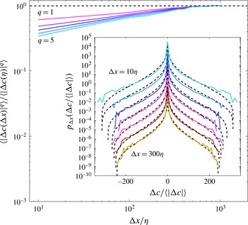
In the regime of minimum self-aggregation, discussed in § 3, concentration values are correlated within stretched lamellae and uncorrelated otherwise. In the correlated domain,
 $\unicode[STIX]{x0394}x<\unicode[STIX]{x1D702}$
, the form of the increment PDF in (2.4) implies that the structure functions should scale as
 $$\begin{eqnarray}\langle |\unicode[STIX]{x0394}c|^{q}\rangle \sim \unicode[STIX]{x0394}x^{q}.\end{eqnarray}$$
For
 $\unicode[STIX]{x0394}x>\unicode[STIX]{x1D702}$
, the structure functions are expected to be constant.
Since the characteristic lamella width
 $\unicode[STIX]{x1D702}=\langle s\rangle$
is very small (of the order of
 $5{-}7~\unicode[STIX]{x03BC}\text{m}$
for the experiment described in § 3), the resolution of the experimental images presented in § 3 do not allow an analysis of the structure functions below
 $\unicode[STIX]{x0394}x=10\unicode[STIX]{x1D702}$
. The measured structure functions in the range
 $10\unicode[STIX]{x1D702}<\unicode[STIX]{x0394}x<300\unicode[STIX]{x1D702}$
show a weak tendency to grow with
 $\unicode[STIX]{x0394}x$
(figure 9). Note that the vertical scale in this figure is the same as for the following figures to emphasize the narrow range of variation of structure functions in this regime. This behaviour is actually not far from the expected constant behaviour, considering that concentration increment PDFs are broad in this regime (see inset of figure 9). In fact, the analytical predictions of (3.18) are in good agreement with the measured concentration increment PDFs for all spatial increments
 $\unicode[STIX]{x0394}x$
. The increment PDFs are broad in this regime, since highly concentrated, weakly stretched, blobs of dye can persist over long distances (see figure 2
a), which induces large concentration increments. The corresponding broad distribution of mixing scales is consistent with the slow convergence of structure functions to a constant value.
Structure functions
 $\langle |\unicode[STIX]{x0394}c|^{q}\rangle$
computed as a function of
 $\unicode[STIX]{x0394}x$
, for
 $q$
ranging from 1 to 5, for the dispersing mixture at position
 $x/d=18$
. The structure functions are normalized by their asymptotic value for large
 $\unicode[STIX]{x0394}x$
,
 $\langle |\unicode[STIX]{x0394}c(\unicode[STIX]{x1D702})|^{q}\rangle$
. The vertical scale is taken as the same for the three regimes allowing for direct comparison of the structure functions (see figures 10 and 11). Inset: concentration increments for
 $\unicode[STIX]{x0394}x=\{10\unicode[STIX]{x1D702},50\unicode[STIX]{x1D702},100\unicode[STIX]{x1D702},200\unicode[STIX]{x1D702},250\unicode[STIX]{x1D702},300\unicode[STIX]{x1D702}\}$
, normalized by their first moment
 $\langle |\unicode[STIX]{x0394}c(\unicode[STIX]{x0394}x)|\rangle$
. The curves are shifted by an arbitrary value for clarity. Simulations are shown as full lines and the analytical solution of (3.17) as dashed lines.

6.2 Fully developed aggregation
When aggregation is significant, structure functions are expected to grow over a large range of scales, since the correlation length
 $\unicode[STIX]{x1D702}$
is much larger than the lamella width (4.4). Following the deconstruction theory presented above, the evolution of concentration increment PDFs with
 $\unicode[STIX]{x0394}x$
is controlled by the scaling of the number of independent aggregated lamella
 $m$
with
 $\unicode[STIX]{x0394}x$
, defined in (2.11). The latter is a function of how the material lines density depends on scale, a dependence characterized by the fractal dimension
 $d_{f}$
.
For fully developed aggregation, as discussed in § 4, the concentration increment PDFs are given by (4.5), which leads to the following expression for their moments,
 $$\begin{eqnarray}\langle |\unicode[STIX]{x0394}c|^{q}\rangle =\frac{2^{q}\unicode[STIX]{x1D703}^{q}}{\sqrt{\unicode[STIX]{x03C0}}\unicode[STIX]{x0393}(m(\unicode[STIX]{x0394}x))}\unicode[STIX]{x0393}\left(\frac{q+2m(\unicode[STIX]{x0394}x)}{2}\right)\unicode[STIX]{x0393}\left(\frac{1+q}{2}\right).\end{eqnarray}$$
For large
 $m\gg 1$
, the structure functions can be approximated by
 $$\begin{eqnarray}\langle |\unicode[STIX]{x0394}c|^{q}\rangle \approx \frac{2^{q}\unicode[STIX]{x1D703}^{q}m(\unicode[STIX]{x0394}x)^{q/2}}{\sqrt{\unicode[STIX]{x03C0}}}\unicode[STIX]{x0393}\left(\frac{1+q}{2}\right).\end{eqnarray}$$
From (2.11), we obtain, for
 $\unicode[STIX]{x0394}x<\unicode[STIX]{x1D702}$
,
 $$\begin{eqnarray}\langle |\unicode[STIX]{x0394}c|^{q}\rangle \sim \frac{2^{q}\unicode[STIX]{x1D703}^{q}}{\sqrt{\unicode[STIX]{x03C0}}}\unicode[STIX]{x0393}\left(\frac{1+q}{2}\right)\unicode[STIX]{x0394}x^{(d_{f}-d+1)q/2}.\end{eqnarray}$$
Hence, in the correlated range, the structure functions scale as
 $$\begin{eqnarray}\langle |\unicode[STIX]{x0394}c|^{q}\rangle \sim \unicode[STIX]{x0394}x^{\unicode[STIX]{x1D709}(q)},\end{eqnarray}$$
with
 $\unicode[STIX]{x1D709}(q)=(d_{f}-d+1)q/2$
, while for
 $\unicode[STIX]{x0394}x>\unicode[STIX]{x1D702}$
, the structure functions are constant since
 $m(\unicode[STIX]{x0394}x)=n$
.
As expected, the scaling of structure functions is directly dependent on the material line fractal dimension
 $d_{f}$
. For space-filling material lines,
 $d_{f}=d$
, and
 $\unicode[STIX]{x1D709}(q)=q/2$
. The evolution of the structure functions with the spatial increment, measured from the turbulent jet experimental data, under confinement by a duct, is in relatively good agreement with the predictions (figure 10). Note that, although the agreement with the full increment PDFs is quite good (inset of figure 10), the match for the structure function is less good for larger orders
 $q$
, which are more sensitive to experimental noise.
Compared to the minimum aggregation scenario (6.2), the exponents
 $\unicode[STIX]{x1D709}(q)$
are reduced by a factor two (6.6). This significant change in structure function scaling quantifies the impact of aggregation on the attenuation of concentration differences. Since the exponent
 $\unicode[STIX]{x1D709}$
are linear with
 $q$
(6.6), scalar fields in this regime do not show intermittent properties. This is also evident from the inset of figure 10, which shows that the shapes of the concentration increments are nearly invariant with
 $\unicode[STIX]{x0394}x$
upon rescaling with
 $\langle |\unicode[STIX]{x0394}c|\rangle$
. As discussed in the following section, the situation is different for non-space-filling material lines that show significant intermittency.
Structure functions
 $\langle |\unicode[STIX]{x0394}c|^{q}\rangle$
computed as a function of
 $\unicode[STIX]{x0394}x$
, for
 $q$
ranging from 1 to 5, for the confined mixture at a distance
 $4L$
from the source. The structure functions are normalized by their asymptotic value for large
 $\unicode[STIX]{x0394}x$
,
 $\langle |\unicode[STIX]{x0394}c(\unicode[STIX]{x1D702})|^{q}\rangle$
. The dashed lines represent the prediction of (6.3), with
 $m(\unicode[STIX]{x0394}x)$
given by (2.12). The vertical scale is taken as the same for the three regimes allowing for direct comparison of the structure functions (see figures 9 and 11). Inset: concentration increments for
 $\unicode[STIX]{x0394}x=\{0.2\unicode[STIX]{x1D702},0.3\unicode[STIX]{x1D702},0.7\unicode[STIX]{x1D702},2.5\unicode[STIX]{x1D702},3\unicode[STIX]{x1D702},3.5\unicode[STIX]{x1D702}\}$
(same curves as in figure 5
b but normalized by the first moment
 $\langle |\unicode[STIX]{x0394}c(\unicode[STIX]{x0394}x)|\rangle$
). The curves are shifted by an arbitrary value for clarity. Simulations are shown as full lines and the analytical solution of (4.5) in dashed lines.

6.3 Partial aggregation
Non-space-filling material lines, which develop in highly heterogeneous flow fields, lead to an extended regime of partial aggregation, as discussed in § 5. Based on expression (5.9), derived for the increment PDFs, the structure functions may be approximated as follows (see appendix B)
 $$\begin{eqnarray}\displaystyle \langle |\unicode[STIX]{x0394}c|^{q}\rangle & {\approx} & \displaystyle [(m-1)\unicode[STIX]{x1D703}]^{q}\frac{\sqrt{\unicode[STIX]{x03C0}}\text{erf}\left[\sqrt{q\ln ((m-1)\unicode[STIX]{x1D703}/\unicode[STIX]{x1D716})}\right]}{2\sqrt{q\ln ((m-1)\unicode[STIX]{x1D703}/\unicode[STIX]{x1D716})}}\nonumber\\ \displaystyle & & \displaystyle +\,\frac{\sqrt{\unicode[STIX]{x03C0}}}{2\sqrt{q\ln [(m-1+q)\unicode[STIX]{x1D703}/\unicode[STIX]{x1D716}]}}\frac{\unicode[STIX]{x1D703}^{q}\unicode[STIX]{x0393}(m+q,m-1)}{\unicode[STIX]{x0393}(m)}.\end{eqnarray}$$
The predictions of (6.7) are in relatively good agreement with the numerical simulations (figure 11). Note, however, that the curves are more noisy for large values of
 $q$
, for which structure functions are more sensitive to experimental noise. For
 $n\gg q$
, the structure functions are
 $$\begin{eqnarray}\langle |\unicode[STIX]{x0394}c|^{q}\rangle \approx [(m(\unicode[STIX]{x0394}x)-1)\unicode[STIX]{x1D703}]^{q}\frac{\sqrt{\unicode[STIX]{x03C0}}}{2\sqrt{q\ln ((m(\unicode[STIX]{x0394}x)-1)\unicode[STIX]{x1D703}/\unicode[STIX]{x1D716})}},\end{eqnarray}$$
which gives, using the scaling
 $m(\unicode[STIX]{x0394}x)\sim \unicode[STIX]{x0394}x^{d_{f}-d+1}$
for
 $\unicode[STIX]{x0394}x<\unicode[STIX]{x1D702}$
,
 $$\begin{eqnarray}\langle |\unicode[STIX]{x0394}c|^{q}\rangle \sim \unicode[STIX]{x0394}x^{\unicode[STIX]{x1D709}(q)},\end{eqnarray}$$
with
 $\unicode[STIX]{x1D709}(q)=(d_{f}-d+1)q$
. The exponent characterizing the scaling of the structure functions with
 $\unicode[STIX]{x0394}x$
, namely
 $\unicode[STIX]{x1D709}=(d_{f}-d+1)q$
differs by a factor
 $1/2$
from that of the full aggregation regime (6.6). Hence, the presence of concentration lacunarities has a strong impact on structure functions, as it tends to promote large concentration differences. Furthermore, the dependence of the structure functions on
 $\unicode[STIX]{x0394}x$
is not exactly a power law, and both the order
 $q$
and the spatial increment
 $\unicode[STIX]{x0394}x$
appear in the pre-factor of the power law in (6.8). This reflects the intermittency observed for the increment PDFs, whose shape evolves as a function of the spatial increment
 $\unicode[STIX]{x0394}x$
(see inset of figure 11). Hence, this regime differs from the fully developed aggregation scenario that showed stable shapes of concentration increment PDFs at different
 $\unicode[STIX]{x0394}x$
(see inset of figure 10). This result provides a theoretical basis for understanding and quantifying the role of the coexistence of concentration lacunarities and dense lamella aggregates on the development of intermittent scalar fields. It suggests that the lack of scaling form of the concentration increment PDFs for different spatial increments, which is a clear signature of intermittency observed here for the partial aggregation case (see the inset of figure 11), can lead to a break down of the power-law behaviour of structure functions. Note that this lack of power-law scaling could potentially be misinterpreted as a nonlinear dependency of the exponent
 $\unicode[STIX]{x1D701}(q)$
on
 $q$
.
Structure functions
 $\langle |\unicode[STIX]{x0394}c|^{q}\rangle$
computed as a function of
 $\unicode[STIX]{x0394}x$
, for
 $q$
ranging from 1 to 5, for the porous media simulation at time
 $t=112.5\unicode[STIX]{x1D70F}_{a}$
(
 $\unicode[STIX]{x1D70E}_{\ln K}^{2}=1$
,
 $Pe=80$
). The structure functions are normalized by their asymptotic value for large
 $\unicode[STIX]{x0394}x$
,
 $\langle |\unicode[STIX]{x0394}c(\unicode[STIX]{x1D702})|^{q}\rangle$
. The predictions of (6.7) are shown as dashed lines. The vertical scale is taken as the same for the three regimes allowing for direct comparison of the structure functions (see figures 9 and 10). Inset: concentration increments for
 $\unicode[STIX]{x0394}x=\{\unicode[STIX]{x1D702}/64,\unicode[STIX]{x1D702}/32,\unicode[STIX]{x1D702}/16,\unicode[STIX]{x1D702}/8,\unicode[STIX]{x1D702}/4,\unicode[STIX]{x1D702}/2,\unicode[STIX]{x1D702},2\unicode[STIX]{x1D702}\}$
(same curves as in figure 8
b but normalized by the first moment
 $\langle |\unicode[STIX]{x0394}c(\unicode[STIX]{x0394}x)|\rangle$
). The curves are shifted by an arbitrary value for clarity. The simulations are shown as full lines and the predictions of (5.9) as dashed lines.

7 Conclusion and further remarks
The distribution of scalar increments in fluids reflects the multiscale spatial correlations that develop in concentration fields as a result of the interplay between diffusion and the repeated stretching actions of the flow. In this study, we have presented a general framework that unravels the spatial structure of scalar fields from the understanding of their basic composition rules. Considering the construction of mixtures as a random aggregation process, with stretched lamellae as elementary aggregated objects, we have developed the corollary concept of random field deconstruction: the difference operator, when applied to a scalar field resulting from diffusive aggregation, dissociates the independent from the common lamellae that contribute to concentration values at neighbouring locations (figure 1
c). We have quantified this phenomenon by deriving the number of independent aggregated lamellae
 $m$
subsisting after differentiation. The latter increases with the spatial increment
 $\unicode[STIX]{x0394}x$
to finally reach the global mean aggregation number
 $n$
at the characteristic correlation length
 $\unicode[STIX]{x1D702}$
.
We have shown through different examples that the increments of a field evolving through a self-convolution process follow the basic rules of deconstruction developed in this study. Their statistics are governed by the random aggregation of
 $m(\unicode[STIX]{x0394}x)$
lamellae, where
 $m(\unicode[STIX]{x0394}x)$
characterizes the scale dependency of lamella density. Based on this theory, general analytical expressions for concentration increments are derived, which are in good agreement with the results of turbulent flow experiments and porous media flow simulations representative of the different possible regimes of aggregation. This framework also yields analytical expressions for structure functions, which allow understanding the origin of different observed scaling behaviours and their consequence for the development of intermittent scalar fields.
We have singled out and studied two distinct, extreme scenarios directing the fate of a mixture: the ever-dispersing mixture, on one hand, is a collection of sheets with distributed, independent histories. The confined mixture, on the other hand, is a stack of sheet bundles which synchronically merge with each other. Natural mixtures may be closer to one or the other of these two caricatures, but will in general incorporate both ingredients, in given relative proportions depending on the way they have been prepared. The partially aggregated fields in § 5 are such examples.
(a) A snapshot of the scalar field in the channel at
 $Re=2000$
showing a bundle of not yet overlapping sheets immersed in an already mixed environment. The two regions (environment and bundle) have
 $n_{1}=27$
and
 $n_{2}=9.7$
, and their relative proportion as in (7.1) is such that
 $f=0.8$
, as shown in (b). (b) PDF of concentrations (full line) corresponding to (a), gamma distribution with
 $n_{1}=27$
(dash-dotted line), gamma distribution with
 $n_{2}=9.7$
(dotted line) and mixed gamma distribution (7.1) with
 $f=0.8$
(dashed line).

Figure 12 shows how a mixture in the channel, close to the entrance section, is itself a mixture of the two idealized cases above. Bundles of not yet overlapping sheets are immersed in an already mixed environment. These two regions, in the language developed in this paper, are characterized by two different values of
 $n$
, one large for the well-mixed region, the other smaller, reflecting the younger age of the not yet mixed bundle of still distinct sheets. The overall concentration PDF is a weighted average of two gamma distributions,
 $$\begin{eqnarray}p_{c}(x=c/\langle c\rangle )=f\frac{n_{1}^{n_{1}}}{\unicode[STIX]{x0393}(n_{1})}x^{n_{1}-1}\text{e}^{-n_{1}x}+(1-f)\frac{n_{2}^{n_{2}}}{\unicode[STIX]{x0393}(n_{2})}x^{n_{2}-1}\text{e}^{-n_{2}x},\end{eqnarray}$$
the fraction
 $f$
standing for the relative proportion of regions with
 $n_{1}$
. Obviously, the increment PDF in that case will be the same weighted average of the increment PDFs in (4.5), each with the appropriate
 $n$
. The overall increment PDF behaviour will be dominated by the contribution of the large
 $n$
(well mixed) regions near
 $\unicode[STIX]{x0394}c=0$
, and its tails will reflect those of the lower
 $n$
regions (incorporating large concentration excursions), thus enhancing the intermittent (broad) character of the PDF. The procedure can thus be applied to a wealth of different situations.
This theoretical framework is expected to be of broad relevance for mixing in fluids, as illustrated here for three different flow fields, including turbulent flows at large Reynolds numbers and porous media flows at low Reynolds numbers. The fact that the developed framework applies equally well to flow fields of very different natures suggests a high degree of universality of its underlying principles. In this framework, the velocity field statistics play an important role in determining the stretching dynamics (e.g. linear, power law or exponential) and the likelihood of lamellae to aggregate, as quantified from the fractal dimension of purely advected material lines. Hence, different velocity field statistics would yield different concentration and concentration increment PDFs. A distinction between intermittent and non-intermittent regimes can be drawn in this framework by analysing the probability of non-space-filling material lines to develop, which leads to partial aggregation and thus intermittency. This probability is linked to the velocity statistics through the fractal dimension
 $d_{f}$
, that depends on the ratio between the dispersion rates, which creates new voids, and the elongation rate, which tends to fill these voids.
The deconstruction theory sheds new light on the significance of increment distributions and provides a way to decipher the composition rules of concentration fields. While the concentration PDF depends only on the current stage of aggregation
 $n$
, the concentration increment PDFs uncovers the different stages of aggregation that have determined the state of a mixture. Spanning through the range of spatial increments
 $\unicode[STIX]{x0394}x$
allows investigating the full range of aggregation stages from the basic elementary lamellae or ‘quantum’ (
 $m=1$
) for small
 $\unicode[STIX]{x0394}x$
to the current stage of aggregation (
 $m=n$
) at large
 $\unicode[STIX]{x0394}x$
.
Finally, we note that the domain of application of the present ideas is likely to extend beyond the context of scalars where it has been conceived, since these ideas naturally apply to any field constructed by the addition of a random variable. In this respect, waves overlapping at random, such as sound waves (Rayleigh 1880), sea waves, capillary waves (Greffier, Amarouchene & Kellay Reference Greffier, Amarouchene and Kellay2002), or the structure of the speckle in optics (Goodman Reference Goodman2007) are, among others, including fracture (Vernède, Ponson & Bouchaud Reference Vernède, Ponson and Bouchaud2015), and turbulent boundary layers (Yang, Marusic & Meneveau Reference Yang, Marusic and Meneveau2016), obvious candidates.
Acknowledgements
T.L.B. acknowledges the support of the European Research Council (ERC) through the project ReactiveFronts (648377) and of the Agence Nationale de la Recherche (ANR) through the project ‘Subsurface Mixing and Reaction’ (ANR-14-CE04-0003). M.D. acknowledges the support of the European Research Council (ERC) through the project MHetScale (617511). E.V. acknowledges the Agence Nationale de la Recherche (ANR) for funding of the ANR-DFG grant TurbMix (ANR-14-CE35-0031-01).
Appendix A. Approximation for the number of independent lamellae contributing to aggregates as a function of the separation distance
 $m(\unicode[STIX]{x0394}x)$

In order to estimate the number of independent lamellae that contributes to concentration values at two positions separated by a distance
 $\unicode[STIX]{x0394}x$
(blue and red curves in figure 1), we quantify the typical scale
 $r(\unicode[STIX]{x0394}x)$
of non-overlap of the two lamella aggregates that determine the respective concentration values (sum of blue and purple curves on the one hand and sum of red and purple curves on the other hand). We first determine the scale of overlap of two lamella aggregates, which are separated by a distance
 $\unicode[STIX]{x0394}x$
. We assume that the concentration across an aggregate whose centre is located at the position
 $\boldsymbol{x}_{i}$
can be represented by the isotropic Gaussian
 $$\begin{eqnarray}p_{a}(\boldsymbol{x}\mid \boldsymbol{x}_{i})=\frac{a^{2}\exp \left(-{\displaystyle \frac{a^{2}|\boldsymbol{x}-\boldsymbol{x}_{i}|^{2}}{4\unicode[STIX]{x1D702}^{2}}}\right)}{4\unicode[STIX]{x03C0}\unicode[STIX]{x1D702}^{2}},\end{eqnarray}$$
where
 $\unicode[STIX]{x1D702}$
is the correlation scale. We set here
 $a=2\sqrt{2}$
. Consider now the line joining the two centres
 $\boldsymbol{x}_{1}$
and
 $\boldsymbol{x}_{2}$
. The distribution of points of overlap along this line may be written as
 $$\begin{eqnarray}p_{ol}(x^{\prime })=\left\{\begin{array}{@{}ll@{}}\frac{\displaystyle \exp \left[-{\displaystyle \frac{2(x^{\prime }-\unicode[STIX]{x0394}x/2)^{2}}{\unicode[STIX]{x1D702}^{2}}}\right]}{\displaystyle \sqrt{\unicode[STIX]{x03C0}\unicode[STIX]{x1D702}^{2}/2}},\quad & x^{\prime }<0,\\ \frac{\displaystyle \exp \left[-{\displaystyle \frac{2(x^{\prime }+\unicode[STIX]{x0394}x/2)^{2}}{\unicode[STIX]{x1D702}^{2}}}\right]}{\displaystyle \sqrt{\unicode[STIX]{x03C0}\unicode[STIX]{x1D702}^{2}/2}},\quad & x^{\prime }>0,\end{array}\right.\end{eqnarray}$$
where we chose the coordinate system aligned with
 $\boldsymbol{x}_{1}-\boldsymbol{x}_{2}$
and origin located at
 $(\boldsymbol{x}_{1}+\boldsymbol{x}_{2})/2$
. The global probability of overlap can then be estimated as
 $$\begin{eqnarray}\displaystyle P_{ol}(\unicode[STIX]{x0394}x) & = & \displaystyle \int _{-\infty }^{\unicode[STIX]{x0394}x/2}\,\text{d}x^{\prime }\frac{\exp \left[-{\displaystyle \frac{2(x^{\prime }-\unicode[STIX]{x0394}x/2)^{2}}{\unicode[STIX]{x1D702}^{2}}}\right]}{\sqrt{\unicode[STIX]{x03C0}\unicode[STIX]{x1D702}^{2}/2}}+\int _{\unicode[STIX]{x0394}x/2}^{\infty }\,\text{d}x^{\prime }\frac{\exp \left[-{\displaystyle \frac{2(x^{\prime }+\unicode[STIX]{x0394}x/2)^{2}}{\unicode[STIX]{x1D702}^{2}}}\right]}{\sqrt{\unicode[STIX]{x03C0}\unicode[STIX]{x1D702}^{2}/2}}\nonumber\\ \displaystyle & = & \displaystyle \text{erfc}\left(\frac{\unicode[STIX]{x0394}x}{\unicode[STIX]{x1D702}}\right).\end{eqnarray}$$
The overlap probability can also be written as
 $P_{ol}=r_{ol}/\unicode[STIX]{x1D702}$
, which is the ratio of the characteristic overlap distance
 $r_{ol}$
to the lamellae size
 $\unicode[STIX]{x1D702}$
. From this, we obtain for
 $r_{ol}$
the expression
 $r_{ol}=\unicode[STIX]{x1D702}\,\text{erfc}\,(\unicode[STIX]{x0394}x/\unicode[STIX]{x1D702})$
. Consequently, the distance
 $r$
of no overlap is given by
 $r(\unicode[STIX]{x0394}x)=\unicode[STIX]{x1D702}-r_{ol}=\unicode[STIX]{x1D702}[1-\text{erfc}\,(\unicode[STIX]{x0394}x/\unicode[STIX]{x1D702})]$
. Thus, we obtain for the number of lamellae in the region of no overlap
 $$\begin{eqnarray}m(\unicode[STIX]{x0394}x)=n\left(\frac{r(\unicode[STIX]{x0394}x)}{\unicode[STIX]{x1D702}}\right)^{d_{f}-d+1}=n\,\text{erf}\,\left(\frac{\unicode[STIX]{x0394}x}{\unicode[STIX]{x1D702}}\right)^{d_{f}-d+1},\end{eqnarray}$$
where
 $n$
is the number of lamellae in the aggregates. Expression (A 4) is equivalent to (2.11) for
 $\unicode[STIX]{x0394}x\ll \unicode[STIX]{x1D702}$
, and converges smoothly to
 $n$
for
 $\unicode[STIX]{x0394}x\gg \unicode[STIX]{x1D702}$
.
Appendix B. Approximation of the concentration PDF for confined dispersing mixtures
In order to obtain an approximation for the PDF (5.3), we perform the variable transform
 $z=x/\unicode[STIX]{x1D703}$
such that
 $$\begin{eqnarray}p_{c}(c)=\int _{c/\unicode[STIX]{x1D703}}^{\infty }\,\text{d}z\frac{z^{n-1}}{\unicode[STIX]{x0393}(n)}\frac{\exp (-z)}{2c\sqrt{\ln (z\unicode[STIX]{x1D703}/\unicode[STIX]{x1D716})\ln (z\unicode[STIX]{x1D703}/c)}}=\int _{c/\unicode[STIX]{x1D703}}^{\infty }\,\text{d}z\frac{1}{\unicode[STIX]{x0393}(n)}\frac{\exp [-z-n^{\prime }\ln (z)]}{2c\sqrt{\ln (z\unicode[STIX]{x1D703}/\unicode[STIX]{x1D716})\ln (z\unicode[STIX]{x1D703}/c)}}.\end{eqnarray}$$
We scale now
 $z=x/n^{\prime }$
, with
 $n^{\prime }=n-1$
, and obtain
 $$\begin{eqnarray}p_{c}(c)=\frac{n^{\prime }\exp [n^{\prime }\ln (n^{\prime })]}{\unicode[STIX]{x0393}(n)}\int _{c/(n^{\prime }\unicode[STIX]{x1D703})}^{\infty }\,\text{d}z\frac{\exp \{-n^{\prime }[z-\ln (z)]\}}{2c\sqrt{\ln (zn^{\prime }\unicode[STIX]{x1D703}/\unicode[STIX]{x1D716})\ln (zn^{\prime }\unicode[STIX]{x1D703}/c)}}.\end{eqnarray}$$
Notice that
 $z-\ln (z)$
has a minimum at
 $z_{0}=1$
. Thus, for
 $c/(n^{\prime }\unicode[STIX]{x1D703})<1$
, we use a saddle point approximation to obtain
 $$\begin{eqnarray}p_{c}(c)\approx \frac{n^{\prime }\exp [n^{\prime }\ln (n^{\prime })-n^{\prime }]}{\unicode[STIX]{x0393}(n)}\int _{c/(n^{\prime }\unicode[STIX]{x1D703})}^{\infty }\,\text{d}z\frac{\exp [-n^{\prime }(z-1)^{2}/2]}{2c\sqrt{\ln (zn^{\prime }\unicode[STIX]{x1D703}/\unicode[STIX]{x1D716})\ln (zn^{\prime }\unicode[STIX]{x1D703}/c)}}.\end{eqnarray}$$
Thus, for
 $n^{\prime }$
sufficiently large, we obtain the approximation
 $$\begin{eqnarray}p_{c}(c)\approx \frac{\sqrt{2\unicode[STIX]{x03C0}n^{\prime }}\exp [n^{\prime }\ln (n^{\prime })-n^{\prime }]}{\unicode[STIX]{x0393}(n)}\frac{1}{2c\sqrt{\ln (n^{\prime }\unicode[STIX]{x1D703}/\unicode[STIX]{x1D716})\ln (n^{\prime }\unicode[STIX]{x1D703}/c)}}.\end{eqnarray}$$
The first term is equal to 1, as is immediate by using Stirling’s approximation. Thus, the PDF can be approximated by
 $$\begin{eqnarray}p_{c}(c)=\frac{1}{2c\sqrt{\ln (n^{\prime }\unicode[STIX]{x1D703}/\unicode[STIX]{x1D716})\ln (n^{\prime }\unicode[STIX]{x1D703}/c)}}.\end{eqnarray}$$
For
 $c/(n^{\prime }\unicode[STIX]{x1D703})>1$
,
 $z-\ln (z)$
is minimum at the lower integral limit
 $c/(n^{\prime }\unicode[STIX]{x1D703})=\unicode[STIX]{x1D6FE}$
. Thus, we now approximate in (B 2)
 $$\begin{eqnarray}z-\ln (z)\approx \unicode[STIX]{x1D6FE}+\ln (\unicode[STIX]{x1D6FE})+\frac{\unicode[STIX]{x1D6FE}-1}{\unicode[STIX]{x1D6FE}}(z-\unicode[STIX]{x1D6FE}).\end{eqnarray}$$
Furthermore,
 $$\begin{eqnarray}\frac{1}{\sqrt{\ln (z/\unicode[STIX]{x1D6FE})}}\approx \sqrt{\frac{\unicode[STIX]{x1D6FE}}{z-\unicode[STIX]{x1D6FE}}}.\end{eqnarray}$$
Thus, we obtain for
 $p_{c}(c)$
by inserting these approximations in (B 2) and executing the remaining integral
 $$\begin{eqnarray}p_{c}(c)=\frac{n^{\prime }\exp [n^{\prime }\ln (n^{\prime })]}{\unicode[STIX]{x0393}(n)}\frac{\exp [-n^{\prime }\unicode[STIX]{x1D6FE}+n^{\prime }\ln (\unicode[STIX]{x1D6FE})]}{2c\sqrt{\ln (\unicode[STIX]{x1D6FE}n^{\prime }\unicode[STIX]{x1D703}/\unicode[STIX]{x1D716})}}\frac{\unicode[STIX]{x1D6FE}}{\sqrt{\unicode[STIX]{x1D6FE}-1}}\sqrt{\frac{\unicode[STIX]{x03C0}}{n^{\prime }}}.\end{eqnarray}$$
Inserting
 $\unicode[STIX]{x1D6FE}=c/(n^{\prime }\unicode[STIX]{x1D703})$
, we obtain
 $$\begin{eqnarray}p_{c}(c)=\frac{c^{n^{\prime }}}{2\unicode[STIX]{x1D703}^{n^{\prime }+1}\unicode[STIX]{x0393}(n)}\frac{\exp (-c/\unicode[STIX]{x1D703})}{\sqrt{\ln (c/\unicode[STIX]{x1D716})}}\frac{\sqrt{\unicode[STIX]{x03C0}/n^{\prime }}}{\sqrt{c/(n^{\prime }\unicode[STIX]{x1D703})-1}}.\end{eqnarray}$$